| Issue |
A&A
Volume 612, April 2018
|
|
|---|---|---|
| Article Number | A40 | |
| Number of page(s) | 11 | |
| Section | Stellar atmospheres | |
| DOI | https://doi.org/10.1051/0004-6361/201732160 | |
| Published online | 17 April 2018 | |
Low-frequency photospheric and wind variability in the early-B supergiant HD 2905
1
Instituto de Astrofísica de Canarias, 38200 La Laguna
Tenerife, Spain
e-mail: This email address is being protected from spambots. You need JavaScript enabled to view it.
2
Departamento de Astrofísica, Universidad de La Laguna, 38205 La Laguna
Tenerife, Spain
3
Instituut voor Sterrenkunde, KU Leuven, Celestijnenlaan 200D
3001 Leuven, Belgium
4
Department of Astrophysics, IMAPP, University of Nijmegen, PO Box 9010
6500 GL Nijmegen, The Netherlands
5
Kavli Institute for Theoretical Physics, University of California, Santa Barbara
CA 93106, USA
6
Institut für Astro- und Teilchenphysik, Universität Innsbruck, Technikerstr. 25/8
6020 Innsbruck, Austria
7
Stellar Astrophysics Centre (SAC), Department of Physics and Astronomy, Aarhus University, Ny Munkegade 120
8000 Aarhus, Denmark
Received:
23
October
2017
Accepted:
6
December
2017
Abstract
Context. Despite important advances in space asteroseismology during the last decade, the early phases of evolution of stars with masses above ~15 M⊙ (including the O stars and their evolved descendants, the B supergiants) have been only vaguely explored up to now. This is due to the lack of adequate observations for a proper characterization of the complex spectroscopic and photometric variability occurring in these stars.
Aim. Our goal is to detect, analyze, and interpret variability in the early-B-type supergiant HD 2905 (κ Cas, B1 Ia) using long-term, ground-based, high-resolution spectroscopy.
Methods. We gather a total of 1141 high-resolution spectra covering some 2900 days with three different high-performance spectrographs attached to 1–2.6m telescopes at the Canary Islands observatories. We complement these observations with the hipparcos light curve, which includes 160 data points obtained during a time span of ~1200 days. We investigate spectroscopic variability of up to 12 diagnostic lines by using the zero and first moments of the line profiles. We perform a frequency analysis of both the spectroscopic and photometric dataset using Scargle periodograms. We obtain single snapshot and time-dependent information about the stellar parameters and abundances by means of the FASTWIND stellar atmosphere code.
Results. HD 2905 is a spectroscopic variable with peak-to-peak amplitudes in the zero and first moments of the photospheric lines of up to 15% and 30 km s−1, respectively. The amplitude of the line-profile variability is correlated with the line formation depth in the photosphere and wind. All investigated lines present complex temporal behavior indicative of multi-periodic variability with timescales of a few days to several weeks. No short-period (hourly) variations are detected. The Scargle periodograms of the hipparcos light curve and the first moment of purely photospheric lines reveal a low-frequency amplitude excess and a clear dominant frequency at ~0.37 d−1. In the spectroscopy, several additional frequencies are present in the range 0.1–0.4 d−1. These may be associated with heat-driven gravity modes, convectively driven gravity waves, or sub-surface convective motions. Additional frequencies are detected below 0.1 d−1. In the particular case of Hα, these are produced by rotational modulation of a non-spherically symmetric stellar wind.
Conclusions. Combined long-term uninterrupted space photometry with high-precision spectroscopy is the best strategy to unravel the complex low-frequency photospheric and wind variability of B supergiants. Three-dimensional (3D) simulations of waves and of convective motions in the sub-surface layers can shed light on a unique interpretation of the variability.
Key words: stars: early-type / rotation / stars: fundamental parameters / stars: oscillations / techniques: spectroscopic
© ESO 2018
1 Introduction
Asteroseismology has progressed immensely over the last decade thanks to the considerable increase in the amount of available high-precision uninterrupted space photometry data (e.g., Chaplin & Miglio 2013; Charpinet et al. 2014; Aerts 2015; Hekker & Christensen-Dalsgaard 2017, for reviews).
Within the first part of this asteroseismic (space) revolution, mainly driven by the MOST, CoRoT, and Kepler missions, massive O-type stars and their evolved descendants, the B supergiants (Sgs), were only serendipitously targeted. As a consequence, just a handful of these stars could be investigated in detail using photometric data from these satellites (Saio et al. 2006; Degroote et al. 2010; Blomme et al. 2011; Briquet et al. 2011; Mahy et al. 2011; Moravveji et al. 2012; Aerts et al. 2010, 2013; Aerts et al. 2017). This has hampered a proper global assessment of the main seismic properties of the early phases of evolution of stars with masses above ~15 M⊙. The situation is expected to improve soon, however, thanks to new observations obtained by the BRITE-Constellation satellites and the K2 mission (see already some examples in Buysschaert et al. 2015, 2017; Pablo et al. 2017). However, the definitive breakthrough in the O star and B supergiant domain will (hopefully) only become a reality after the launching of the TESS and PLATO space missions.
Meanwhile, important advances can be also achieved using ground-based time-resolved spectroscopy (e.g., Kraus et al. 2015; Aerts et al. 2017). Indeed, these complementary observations will become decisive for disentangling the intricate – and most likely interconnected – photospheric and wind variability present in the whole massive star domain (see Ebbets 1982; Prinja et al. 1996; Fullerton et al. 1996; Kaufer et al. 1996, 1997; Rivinius et al. 1997; Morel et al. 2004; Markova et al. 2005, 2008; Martins et al. 2015, for some illustrative examples). Such data are in any case needed to perform a reliable seismic characterization of these extreme stellar objects. For this reason, we started long-term spectroscopic monitoring of about 20 bright Galactic O stars and B Sgs using the high-resolution spectrographs attached to the Nordic Optical Telescope (NOT 2.56m), the Mercator 1.2m telescope, and the Hertzsprung-SONG 1m telescope, all of them operated in the Canary Islands observatories1. The first results from this collaboration were presented in Aerts et al. (2017), where we focused on the detection, analysis, and interpretation of the photospheric and wind variability of the late-O supergiant HD 188209 as deduced from Kepler space photometry and long-term high-resolution spectroscopy. Here, we investigate variability in the early-B-type Supergiant HD 2905 (κ Cas, B1 Ia), mainly using ground-based high-resolution spectroscopy obtained over a time period of ~2900 days.
The paper is structured as follows. After describing the main characteristics of the compiled spectroscopic dataset in Sect. 2, we summarize the mean stellar parameters and abundances of HD 2905 in Sect. 3. This work mostlyconcentrates on the characterization of the spectroscopic variability present in this early-B Supergiant; however, we also analyze the available hipparcos light curve to investigate its photometric variability. The results obtained from both independentanalyses are presented in Sect. 4, while we provide a discussion on the physical interpretation of the observed variability in Sect. 5.
2 Observations
The bulk of the observations considered in this paper were gathered in the framework of the IACOB project (Simón-Díaz et al. 2011, 2015). Our monitoring of HD 2905 started with a couple of four-night runs with the FIES instrument (Telting et al. 2014)attached to the 2.56-m Nordic Optical Telescope (NOT, Observatorio del Roque de los Muchachos, La Palma, Spain). These spectra were used in Simón-Díaz et al. (2010) to investigate the possible connection between macroturbulent broadening and line-profile variations in OB supergiants. HD 2905 was one of the targets in the sample for which large spectroscopic variability was detected, with a peak-to-peak amplitude of the first moment2 of the Si III λ4552 line somewhat larger than 10 km s−1. We hence decided to carry on with the spectroscopic monitoring of this star, performing several additional dedicated runs with the HERMES spectrograph (Raskin et al. 2011) attached to the 1.2-m Mercator telescope (Observatorio del Roque de los Muchachos) and the échelle spectrograph attached to the prototype 1-m Hertzsprung-SONG node (Grundahl et al. 2007, 2014) operational at Observatorio del Teide (Tenerife, Spain).
Particular effort was made to assemble an overall spectroscopic dataset that contains stable high-precision spectroscopy with a long time base (FIES and HERMES data), as well as high cadence (SONG) spectroscopy. These two aspects are essential if one wants to achieve an overall view of long-term low-amplitude supergiant variability (see, e.g., Aerts et al. 2017).
A summary of the spectroscopic observations used in this work can be found in Table 1. We first provide information about the separated runs and then the global characteristics of the dataset associated with each instrument. We also present a visual overview of the compiled observations in Fig. 1. We gathered a total of 1141 high-resolution (R) high signal-to-noise (S/N) spectra over a time period of 2900 days separated in various observing runs ranging from 3 days to about 1 month. Most of these observing runs correspond to HERMES and FIES spectra obtained in low cadence mode (5–15 spectra per night with a separation of 1–2 h during 3–10 nights – see, e.g., panel B in Fig. 1). We also benefited from the much more versatile operational mode of the SONG telescope to perform two runs in high cadence mode (8 and 11 consecutive nights, respectively, with a cadence of ~8 min and almost full night coverage – see, e.g., panels C and D in Fig. 1). The second SONG high cadence run was allocated just after a longer SONG low cadence mode (21 nights, 2–3 spectra per night). In all cases, HD 2905 was observed when the star had a visibility of at least 3 h and a maximum of ~10 h.
The observing strategy was different between the SONG and FIES+HERMES campaigns. In the former, the exposure time was fixed to480 s. This resulted in a S/N ranging from 75 to 200 depending on the altitude of the star and the sky conditions. In the latter, we use the exposure tool available at the telescope to end up with a spectrum with S∕N ~ 200–300. This implied a typical exposure time of ~150 s (FIES) and ~200 s (HERMES) and a range in this quantity of 100–500 s depending on the sky conditions when the star was observed.
Our on-ground spectroscopic observations were complemented with the publicly available hipparcos light curve of HD 2905 containing 160 datapoints assembled over ~3.2 yr (see details in the last row of Table 1).
Summary of the spectroscopic and hipparcos observations used in this work.
3 Mean stellar parameters and abundances
Given the visual magnitude of HD 2905 (V = 4.16 mag), this star occurs in most of the studies investigating the physical properties of relatively large samples of Galactic B supergiants (see, e.g., McErlean et al. 1999; Kudritzki et al. 1999; Crowther et al. 2006; Searle et al. 2008). In this paper, we performed our own determination of the basic stellar and wind parameters, as well as abundances with a twofold objective. We wanted to (1) revisit the outcome from the quantitative spectroscopic analysis of this early-B supergiant using observations of much better quality than previous studies and (2) investigate whether the detected spectroscopic variability is also reflected in the quantities resulting from the analysis of individual spectra.
To this aim, we considered the 56 spectra corresponding to the HERMES-2 run (see Table 1 and the second row in Fig. 1) and one additional spectrum with a much higher S/N obtained from adding all these spectra. For the estimation of the stellar+wind parameters and abundances we relied on the non-LTE atmosphere/spectrum synthesis code FASTWIND (Santolaya-Rey et al. 1997; Puls et al. 2005; Rivero González et al. 2011) and a quantitative spectroscopic analysis strategy. Prior to the FASTWIND analysis, we used the IACOB-BROAD tool (Simón-Díaz & Herrero 2014) to perform a line-broadening analysis of the Si III λ4552 line in each of the 56 individual and the averaged spectra in order to obtain estimates for the projected rotational velocity (v sin i) and the amount of macroturbulent broadening (vmac).
In addition to vsini and vmac , the other quantities directly obtained from the spectroscopic analysis are the effective temperature (Teff ), the stellar gravity (log g), the wind-strength parameter (Q) and the exponent of the wind-velocity law (β), plus the microturbulence (ξt) and the absolute helium, silicon, oxygen and magnesium surface abundances. To obtain estimates of all these quantities, we basically followed the same fitting strategy (including the set of diagnostic lines) as described in Urbaneja et al. (2017) and utilized a similar grid of FASTWIND models (but for solar metallicity). Despite some degree of variability in the derived values of the two line-broadening parameters (see Table 2), we decided to fix these two quantities to v sin i = 58 km s−1 and vmac = 82 km s−1 in the FASTWIND analysis of the complete dataset.
The spectroscopic parameters were then combined with information about the terminal velocity (v∞ ) of the stellar wind and the absolute magnitude in the V -filter (MV ) to obtain estimates for the stellar radius (R), mass-loss rate (Ṁ) and luminosity (L). In particular, we adopted the robust UV determination of the wind velocity inferred by Prinja et al. (1990) and Howarth et al. (1997) from the analysis of the IUE high-resolution spectrum of this star (v∞ = 1105 km s−1) and the nominal distance modulus to Cas OB14 (to which HD 2905 belongs) proposed by Humphreys (1978). This distance (m–M = 10.2) was then combined with our own estimation3 of the extinction in the V filter (Av) to end up in MV = −7.1 mag.
Table 2 summarizes the outcome of our quantitative spectroscopic analyses applied to the averaged and individual spectra, respectively. We indicate in the second and third columns the central values and associated uncertainties resulting from the analysis of the averaged spectrum, respectively. The fourth, fifth, and sixth columns quote the mean and standard deviation (as well as the minimum and maximum values), respectively, obtained from the individual 56 spectra of the HERMES-2 run. The latter, once compared with the intrinsic uncertainties of the analysis strategy, provides a rough indication of potential variability in the derived parameters. The above mentioned information is complemented with Fig. 2, where we show the quality of the final fit of the corresponding FASTWIND synthetic spectrum to one of the analyzed spectra. In addition, and for comparison purposes, we also include the set of stellar parameters and abundances obtained by Crowther et al. (2006) and Searle et al. (2008), based on the analysis of an intermediate resolution spectrum covering a more limited wavelength range (Lennon et al. 1992)with the stellar atmosphere code CMFGEN (Hillier & Miller 1998; Hillier et al. 2003). The agreement between the results from the analysis of the combined spectrum (central values and formal uncertainties) and the time-series (mean values and standard deviation) is remarkably good. However, there is a non-negligible scatter in the quantities resulting from the analysis of the individual spectra that may be pointing towards a real variability in the derived parameters and abundances.
Stellar+wind parameters and abundances of HD 2905.
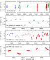 |
Fig. 1 Summary of spectroscopic observations compiled for HD 2905 with the FIES (blue), HERMES (green), and SONG (red) spectrographs. The various panels show the variability of the first normalized moment (centroid in velocity) of the Si III λ4552 line. |
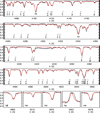 |
Fig. 2 Portions of the spectrum of HD 2905 showing the quality of the fit of the FASTWIND synthetic spectrum (red) to one of analyzed spectra (black). The main diagnostic lines providing information about stellar parameters, abundances and/or spectroscopic variability are also indicated. |
4 Detection and characterization of the stellar variability
4.1 Photometric variability
In contrast to the case of HD 188209 discussed in Aerts et al. (2017), we do not have high-cadence space photometry at our disposal. We thus considered the hipparcos light curve as the best alternative to investigate the photometric variability. Despite the fact that it only allows to search for variability at mmag level, the hipparcos data proved to be a suitable resource to find gravity-mode pulsations of such amplitude in evolved hot supergiants (e.g., Lefever et al. 2007).
The morphology of the Scargle periodogram (Fig. 3) is quite different from the ones of β Cep pressure-mode pulsators (e.g., Aerts 2000) but does bear some resemblance to those of slowly pulsating B stars, for which the dominant coherent gravity-mode pulsations can be retrieved from hipparcos photometry (De Cat & Aerts 2002). Unlike for those stars, however, the hipparcos periodogram of HD 2905 shows a clear amplitude excess at frequencies below 4 d−1 from which a few significant frequencies stand out. We note that the second amplitude bump located between 8 and 14 d−1 is a consequence of the limited sampling of the HIPPARCOS data, which produces a spectral window as in the inset of Fig. 3. The periodogram resembles that of HD 188209 (Fig. 4 in Aerts et al. 2017), where we also showed how the photometric amplitude spectrum of that late-O supergiant improves when relying on Kepler scattered-light photometry with a similar time-span as the hipparcos dataset but with a much higher cadence (the number of data points is ~200 times larger).
On top of the general amplitude bump excess at low frequencies found from the hipparcos data, we find a dominant isolated frequency peak at f1 = 0.37786 ± 0.00001 d−1, with an amplitude of 18 ± 2 mmag (see dashed line in the main panel of Fig. 3). A fit in the time domain shows its first harmonic 2f1 to have a significant amplitude as well, of value 9 ± 2 mmag (this peak is buried within a forest of additional peaks in the black curve in Fig. 3). After prewhitening a harmonic fit with f1 and 2f1 , shown in Fig. 4 as the red line, we find a second frequency f2 = 0.13813 ± 0.00001 d−1 in the residuals (indicted by the blue dotted line in the left inset of Fig. 3), with an amplitude of 14 ± 2 mmag. Further prewhitening leads to  = 11.27175 ± 0.00002 d−1 (located outside the frequency range shown in the left inset of Fig. 3), with an amplitude of 8 ± 2 mmag. After prewhitening this third frequency, we no longer find significant frequencies adopting the common criterion of accepting a frequency if its amplitude is above four times the average noise level in an oversampled periodogram (Breger et al. 1993). Even though it fulfils the noise criterion, the reliability of
  is not at a similar level as the other two detected frequencies, especially since it is located in a region of the Scargle periodogram affected by the aliasing in the hipparcos data. The harmonic fit to the hipparcos photometry with f1 and f2 explains a fraction of 74% of the variability in that light curve.
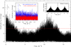 |
Fig. 3 Amplitude spectrum of the hipparcos light curve of HD 2905, where the dominant frequency peak (f1 ) is also indicated. The right inset represents the spectral window. The left inset is a zoom of the amplitude spectrum showing two subsequent levels of prewhitening and the only additional reliable frequency peak (f2 ) standing out above four times the average noise level, indicated by the horizontal red dashed line (see text for details). |
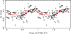 |
Fig. 4 hipparcos light curve folded according to the dominant frequency. The red line is the fit for f1 and its first harmonic. |
4.2 Spectroscopic variability
Subsequently, we turned to the time-resolved spectroscopy. Compared to the study of HD 188209 performed in Aerts et al. (2017), more spectral lines were available for the investigation of spectroscopic variability thanks to the somewhat lower effective temperature of HD 2905. In the HERMES and FIES spectra we had access to 13non-blended – and strong enough – spectral lines; among which there is Si III, Si IV, O II, He I, Hβ , and Hα . In the SONG spectra, some of these lines are missing, mainly due to the more limited wavelength coverage in the blue. In particular, the SONG spectra lack the Si IV λ4116 line, an important diagnostic line to establish the effective temperature of the star. Additional interest in this line comes from the fact that, in early-B supergiants, it is formed in deeper regions of the stellar photosphere compared to Si III, O II, and He I lines.
Following the strategy described in Aerts et al. (2017), we computed the equivalent width (EW; moment of order zero expressed in Å) and the centroid (first moment, denoted as ⟨v⟩ expressed in km s−1) for each of the lines and for each of the three spectroscopic datasets listed in Table 1. By way of example, we show the EW and ⟨v⟩ of the Si III λ4552Å line in Fig. 5; this line is the deepest one of a triplet and was shown to be an optimal line-profile diagnostic for low-amplitude variability of stars with similar temperature to HD 2905 (e.g., Aerts & De Cat 2003). Despite careful normalization of all the spectra, it can be seen in the top panel of Fig. 5 that there are non-negligible differences in the EW resulting from the three different spectrographs. This was already stressed in Aerts et al. (2017) and implies that simply merging datasets is not optimal when hunting for low-amplitude variability. Thanks to the definition of the line moments adopted in Aerts et al. (1992), differences in EW are compensated for in ⟨v⟩, as can be seen in the bottom panel of Fig. 5. Nevertheless, small differences due to the different instruments and atmosphericconditions cannot be excluded, so we continued with the three separate datasets as well as with their merged versions.
4.2.1 Variability of zero and first moments of the line profiles
A detailed look at Figs. 1 and 5 reveals complex temporal behavior of the Si III λ4552 line profile of HD 2905. The star is a clear spectroscopic variable with peak-to-peak amplitudes in equivalent width and the first moment of this line up to 15% and 30 km s−1, respectively.We also conclude that we are dealing with multi-periodic variability, with timescales of a few to several days, in qualitative agreement with f1 and f2 found in thehipparcos photometry. Visual inspection of the SONG high-cadence observations (e.g., bottom panel in Fig. 1) does not reveal short-period variations. This leads us to conclude that any frequency peak detected in the hipparcos periodogram above 2 d−1 is likely spurious and a consequence of the relatively poor time sampling of those photometric data.
In the following, we concentrate on data obtained during the HERMES-2 run (10 nights; see second panel in Fig. 1) to illustrate the main conclusions that can be extracted from the qualitative investigation of the temporal behavior of the EW and centroid of the whole set of considered diagnostic lines. As indicated above, we rely on this subset of spectra due to the availability of the Si IV λ4116 line. Figures 6 and 7 show the detected variability from two different perspectives. On the one hand, Fig. 6 serves to illustrate whether there exist correlations between temporal variations in the first moment of the various lines. On the other hand, Fig. 7 allows a direct comparison of variability in EW and ⟨v⟩ as a function of time for a subset of lines. For better visualization, we divide the results presented in Fig. 6 in three panels including, from top to bottom, metallic lines, He I lines, and Hα and Hβ . We use Si III λ4552 as a baseline and refer all obtained values of ⟨v⟩ per line to the one corresponding to the first spectrum in the HERMES-2 time-series. This way we eliminate potential shifts in velocity between the different lines due to atomic data (central wavelengths). Inspection of Fig. 6 leads us to conclude that there is a fair correlation between variability of ⟨v⟩ in all those lines which are mainly formed in the same regions of the photosphere, that is, all Si III and O II lines, plus all He I lines except for He I λ5875. The latter, similarly to Hα and Hβ , seems to behave in a different way and presents much greater variability. Last, there is a clear positive correlation between the temporal variation of the centroid of the Si III λ4552 and Si IV λ4116 lines, but the amplitude of variability is much smaller in the latter.
Figure 7 shows the Si III λ4552 and Si IV λ4116 photospheric lines, and three additional lines (partially) formed in the stellar wind (He I λ5875, Hβ and Hα ), and also includes the equivalent widths. As indicated above, all lines show clear variability in EW and ⟨v⟩ on time scales shorter than the considered 10 days. The equivalent widths and the centroids of the lines seem to vary more or less in anti-phase of each other, but not always. Again, we see that the amplitude of variability increases from the Si IV line to Hα , passing by the Si III line, He I λ5875, and Hβ . A correlationis found between the amplitude of variability of the lines and how deep they are formed in the stellar photosphere+wind. This is entirely similar to the case of HD 188209 (Aerts et al. 2017).
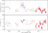 |
Fig. 5 Equivalent width (EW, top) and centroid of the line (⟨v⟩, bottom) of the Si III λ4552 line. Blue: FIES, red: SONG, green: HERMES. |
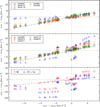 |
Fig. 6 Correlations in the temporal variability of the first moment (centroid) of 13 diagnostic lines in HD 2905. The Si III λ4552 line is used as baseline (x-axis) and all measurements are referred to the value of ⟨v⟩ (per individual line) corresponding to the first spectrum in the HERMES-2 dataset (see also Table 1 and Fig. 7). |
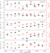 |
Fig. 7 Illustrative example of temporal variability of the zero (EW, red open circles) and first moment (⟨v⟩, black filled circles) of five representative diagnostic lines in HD 2905. The time baseline corresponds to the 10 nights of observationsobtained in the HERMES-2 run (see also Table 1 and Fig. 6). |
4.2.2 Frequency analysis
We computed Scargle periodograms (Scargle 1982) of the EW and ⟨v⟩ of all 13 spectral lines for each of the three FIES, HERMES, and SONG data sets, as well as for the merged sets. Figures 8 and 9 illustrate our findings for the individual datasets for the Si III λ4552 and Hα lines, respectively.Similar results in terms of global morphology of the Scargle periodograms and detected frequencies are found for the various lines included within one of the two groups discussed above (i.e., mostly photospheric or partially formed in the wind) for which Si III λ4552 and Hα can be considered as representative, respectively.
The first conclusion that can be extracted from inspection of the individual Scargle periodograms is that the FIES dataset alone is not enough to provide any reliable information, despite being the one with the longest time-span ( ≈2800 days, see Table 1). This is due to the extremely low duty cycle of these observations. On the contrary, the time sampling achieved with HERMES and SONG results in much cleaner periodograms, although still affected by an important 1-day alias feature, a common phenomenon for single-site data. Interestingly, both lead to a similar conclusion as the one inferred from the Scargle periodogram associated with the hipparcos photometry: the detected variability – this time in EW and ⟨v⟩ – is concentrated at low frequencies. In addition, the better sampling of the hourly time-scales in this case helps to confirm that the amplitude excess found in the frequency range 6–14 d−1 in the hipparcos periodogram (Fig. 3) is spurious, as was already suspected from visual inspection of the SONG high-cadence observations (Sect. 4.2.1 and Fig. 1).
At firstglance, the HERMES and SONG periodograms of the EW of Si III λ4552 (left panel in Fig. 8) do not lead to one and the same dominant frequency. The amplitude excess is mainly concentrated below ~0.4 d−1 . Due to daily aliasing, this feature is then repeated in the ranges 0.6–1.4 and 1.6–2.4 d−1 with decreasing amplitude. A similar result is found for the EW of all the other investigated lines, as well as for the first moment of He I λ5875, Hβ , and Hα (see Fig. 9 for the case of Hα). The SONG-⟨v⟩ periodograms of the purely photospheric lines all reveal a dominant frequency (see, e.g., right panel in Fig. 8). Its actual value is slightly different for the different spectral lines, but is always between 0.36 and 0.39 d−1 , entirely consistent with f1 in the hipparcos data. This frequency is also present in the corresponding HERMES-⟨v⟩ periodograms, but not always with the maximum amplitude. In addition, the amplitude excess at lower frequencies is somewhat broader in the periodogram obtained from the HERMES-⟨v⟩ dataset (compared to SONG-⟨v⟩, see middle and bottom right panels in Fig. 8).
Similarly to Aerts et al. (2017), we also computed multiplied Scargle periodograms by considering the geometric mean per frequency; that is, we multiplied the individual periodograms after rescaling each one of them such that the dominant peak receives value 1, and took the cube root. This method optimally exploits the different structures of the periodograms of FIES and HERMES, where the long-term stability and time base are the asset, as well the high cadence of the SONG spectroscopy. This multiplied periodogram is compared with the one obtained from the merged ⟨v⟩ data for the Si III line at 4552Å and Hα in Fig. 10. The overall morphology of the four periodograms is consistent and points again to low-frequency amplitude excess (below ~0.45 and ~0.25 d−1 for Si III λ4552 and Hα , respectively) that is replicated at higher frequencies due to daily aliasing.
Interestingly, the peak at ~0.37 d−1, dominant in the merged periodogram of Si III λ4552 (and marked with a red thick dashed line), becomes much weaker in the multiplied periodograms. Further, a new frequency peak at ~0.05 d−1 (blue thick dashed line) becomes dominant in the latter. This peak is also present in the periodogram of the Hα line, competing in amplitude with two others at ~0.013 and 0.09 d−1 (green and yellow thick dashed lines, respectively). These four peaks, along with many other additional ones with lower amplitude – but clearly above four times the average noise level in the range 5–15 d−1 – shape the low-frequency amplitude excess characterizing the variability of HD 2905.
Aerts et al. (2017) further investigated the nature of variability of the O9 Iab star HD 188209 by computing short-time Fourier transformations (STFTs) of the Kepler scattered light photometry. This was possible thanks to the unprecedented space photometric dataset obtained at high cadence for this star. Such STFTs allow to decide whether we are dealing with multi mode beating of stable phase-coherent non-radial pulsation modes (see, e.g., Fig. 5 in Degroote et al. 2012) and/or a dominant base frequency due to rotational modulation (Degroote et al. 2011), or rather variability produced by a stochastic phenomenon. Examples of the latter can be found in Tkachenko et al. (2012, Fig. 3), Blomme et al. (2011, Fig. 6) and Aerts et al. (2017, Fig. 5). Unfortunately, our spectroscopic dataset is not suitable for an STFT analysis due to too low a cadence for the longest-term datasets.
The TESS mission will offer a good opportunity to obtain the appropriate time-resolved space photometry4 of HD 2905 to be able to compute meaningful STFTs. Meanwhile, we present in Fig. 11 a comparison of various Scargle periodograms obtained from several of the HERMES and SONG individual runs (see Table 1), as well as the complete dataset. We indicate, for reference, the two dominant peaks found in the merged and multiplied periodograms for the first moment of the Si III λ4552 line (0.3686 and 0.0558 d−1, respectively). While no firm conclusions can be extracted about the temporal stability of the dominant frequency peaks, as anticipated, Fig. 11 illustrates the importance of assembling an overall spectroscopic dataset that contains high cadence spectroscopy interlaced in between lower cadence runs with a time base of several years.
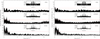 |
Fig. 8 Scargle periodograms of the EW (left) and ⟨v⟩ (right) of the individual datasets for the Si III λ4552 line. The corresponding spectral windows are also included as insets. Red horizontal dashed lines indicate four times the average noise level in the range 5–15 d−1 . |
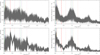 |
Fig. 10 Multiplied Scargle periodograms (top panels) of all three individual FIES, HERMES, and SONG datasets, after rescaling each one of them to their dominant frequency (see text), compared with the periodogram of the merged dataset (bottom panels) for the first moment of the Si III λ4552 (left) and Hα (right) lines.Thick dashed lines indicate some of the dominant frequencies identified in any of the four periodograms. Thin dotted lines show their ±1 day aliases. |
4.2.3 Line-profile variability
In order to further interpret the dominant line-profile variability, which occurs on time scales of at least a few days, without relying on integrated quantities such as the equivalent width or centroid velocity, we increased the S/N of the individual spectral lines by averaging 16 consecutive SONG spectra. In that way, the S/N is upgraded with a factor 4 and the integration time is between 3 and 4 h, which is still only 5% to 7% of the dominant periodicity found in the hipparcos and SONG data. The results of such averaging are represented for four spectral lines in Fig. 12, where the black/red lines are for the first/second intensive SONG campaigns. In this way, line-profile variability is prominentlyrevealed, a typical situation for pulsations of hot massive stars when studied in spectroscopy of S/N above 250.
All spectral lines vary consistently with each other and lead again to the conclusion that HD 2905 has complex multi-periodic line-profile variability. The variability is dominantly present in the blue spectral line wing for the first SONG campaign but in the right line wing during the second SONG run. Despite the presence of telluric lines in the He I line, we find the same results for that line and also for Hβ, which are both formed partially in the stellar wind. This is empirical evidence that the line-profile variability originates in the photosphere but persists in the wind and occurs with a multiple beating phenomenon that is longer than a week.
Further insight into the characteristics of the spectroscopic variability present in HD 2905 can be obtained from the investigation of the residuals in λ-space (i.e., wavelength space) of the various diagnostic line profiles. To this aim, we computed the mean line profile using the complete HERMES+FIES+SONG dataset and divided each of the individual lines by this mean profile. In the case of the SONG spectra obtained in high cadence mode, as mentioned above, we averaged the resulting residual spectrum within a time-slot of ~2 h (i.e., 16 spectra) to increase the S/N. Figure 13 presents three cases of lines formed in different regions of the stellar photosphere+wind. The figure shows the observations gathered in June/July 2016 (HJD = 2 457 576–2 457 617 d), which include the HERMES-4 (4 nights, low cadence), FIES-3 (3 nights, low cadence), SONG-2 (20 nights, low cadence) and SONG-3 (10 nights, high cadence) campaigns. When joined together, they can be considered as the longest observing run with (almost) full coverage of consecutive nights. Apart from the temporal distribution of residuals in λ-space (central panels), we show the centroid velocity curve (⟨v⟩, left panels) and some illustrative line-profiles (bottom panels) for a few selected dates. As a reference, we overplot in each of the diagrams three sinusoidal curves corresponding to three different frequencies. The first two are the dominant peaks found in the merged and multiplied periodograms of the complete spectroscopic dataset for the Si III λ4552 line; that is, 0.055 and 0.369 d−1, respectively (see left panel in Fig. 10). This second frequency is the dominant one in the hipparcos photometry. The third one (0.019 d−1) refers to the dominant frequency standing out from the analysis of the first moment of the Hα line during the ≈40 nights5 considered in Fig. 13.
Once more, the diagrams presented in Fig. 13 show the complex multi-periodic variability characterizing the line profiles of HD 2905. Apart from the almost perfect resemblance of the residuals of the Hα and Hβ lines (despite one being in emission and the other in absorption) the periodicity associated with the frequency of 0.055 d−1 ( ≈18 d, pink curves) seems to be a common feature in the residuals of all analyzed lines, independently of where they are formed in the outer layers of the star. In addition, while spectroscopic signatures related to the other two quoted frequencies seem to be present in the ⟨v⟩-curves of the three lines, 0.369 d−1 ( ≈2.7 d, purple curves) dominates the temporal behavior of the photospheric lines and the photometry, while the large-scale wind variability is mainly modulated by the frequency 0.019 d−1 ( ≈50 d, blue curves).
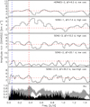 |
Fig. 11 Scargle periodograms of the first moment of the Si III λ4552 line from several of the HERMES and SONG individual runs (see Table 1) and the complete dataset (bottom panel, see notes in Fig. 10). |
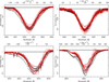 |
Fig. 12 Line profiles averaged over 16 individual consecutive measurements of the SONG spectroscopy of the first (black) and second (red) intensive campaigns. The top two panels are for photospheric lines (left: Si III, right: O II) while the bottom two panels are for lines affected by the stellar wind (left: He I with sharp dips caused by telluric lines, right: Hβ ). |
5 Discussion
Single-site6 spectroscopy of the B1Ia star HD 2905 gathered over a time period of ~7 yr in campaigns with a duration of 4–20 nights reveal empirical evidence of photospheric and wind variability with periodicities of a few to several days. One dominant frequency of ~ 0.37 d−1 was found in both the hipparcos space photometry and in the photospheric spectral lines. Aside from this frequency, HD 2905 reveals multi-periodic spectroscopic variability. The overall peak-to-peak amplitude in the zero and first moments of the photospheric lines reaches up to 15% and 30 km s−1, respectively.The variability increases in amplitude from lines formed deep in the photosphere to those formed in the stellar wind. This property was also found for the O9.5Iab star HD 188209 (Aerts et al. 2017).
The firstmoments of the Si III λ4552 and Hα lines of HD 2905 reveal variations with frequencies below ~0.4 and ~0.1 d−1, respectively. In addition, several frequency peaks located in the range ~0.02–0.4 d−1 occur on top of a global amplitude excess in the various periodograms. The frequencies below ~0.05 d−1 have a large amplitude in the periodograms of the Hα line. If we assume veq = 60 km s−1 and R = 40 R⊙ (see Table 2), we obtain Prot = 34 d (or, equivalently, frot = 0.029 d−1). Taking intoaccount that we are actually measuring veq sin i, but also that there is some empirical evidence indicating that our current techniques to derive projected rotational velocities in B supergiants lead to upper limits of this quantity (Simón-Díaz & Herrero 2014), we assess that any rotational variability should occur in the frequency domain below ≈0.1 d−1 . Therefore, the two dominant frequency peaks located at ≈0.019 and ≈0.055 d−1 (see Sect. 4.2.2 and Figs. 10 and 13) could be related to the rotation of the star. The longer-term variability among these two ( ≈50 d) is only detected in the Hα line, which must be formed in the stellar wind as it permanently reveals strong emission. This result, combined with the time-dependent behavior of its shape, points to a rotationally modulated non-spherical stellar wind as the main cause of this aspect of the detected variability. Line-profile variability associated with the second low-frequency peak at ≈0.055 d−1 ( ≈20 d) is detected in the residuals of Hβ and the Si III λ4552 line (see Fig. 13). Indeed, this frequency dominates in the multiplied Scargle periodogram of this latter line (see left panel in Fig. 10). Therefore, rotational modulation may also explain part of the variability detected in lines formed in the photosphere, while these lines are dominated by shorter-term variability at ~ 0.37 d−1 and other candidate frequencies above 0.1 d−1.
Whether or not the photospheric variability of HD 2905 found in the range ≈0.1–0.4 d−1 (see Fig. 10) is of stochastic nature remains to be studied. Aside from this, the quasi-stable frequency ~ 0.37 d−1 seems to point towards a phenomenon of coherent variability as it persists over years in both the spectroscopy and the space photometry. A combination of stable heat-driven gravity modes (Godart et al. 2017) with convectively driven stochastic gravity waves excited in the stellar interior – either in the convective core (Aerts & Rogers 2015) or in the convection zone in the stellar envelope due to the iron opacity bump (Grassitelli et al. 2015) – seems to offer the best explanation for the complex variability detected in the spectroscopy of HD 2905.
As in the study of the late O supergiant HD 188209 by Aerts et al. (2017), uninterrupted high-cadence space photometry combined with long-term high-precision spectroscopy is the best strategy to tackle the full interpretation of the complex variability of B supergiants. In this work, we managed to distinguish between the weeks-long wind variability and the days-long photospheric variability. Moreover, we found the latter to propagate into the lower part of the stellar wind. In order to understand the full cause of the photospheric variability, three-dimensional simulations of gravity waves on the one hand and of convection in the sub-surface layers on the other hand are needed. The frequency spectra of the photospheric motions predicted by these two distinct phenomena can then be compared with the measured frequency spectra of a large sample of blue supergiants to come to a robust physical interpretation of the overall variability.
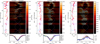 |
Fig. 13 Temporal distribution of residuals in λ-space for three representative line profiles in HD 2905. (Left) Si III λ4567 as an example of a purely photospheric line. (Right) Hα as the most extreme case of optical line affected by stellar wind. (Middle) Hβ as an intermediate case. We also include for reference purposes three sinusoidal curves with associated frequencies 0.055 d−1 (pink), 0.019d−1 (blue), and 0.369 d−1 (purple), respectively (see Sect. 4.2.3 for discussion). Panels to the left show the temporal variation of the centroid of each line-profile (⟨v⟩). Bottom panels include several individual profiles corresponding to the dates indicated as horizontal lines in the left panels, as well as the mean profile obtained from the complete FIES+HERMES+SONG spectroscopic dataset. |
Acknowledgements
This study is based on observations made with the Nordic Optical Telescope, operated by NOTSA, and the Mercator telescope, operated by the Flemish Community, both at the Observatorio del Roque de los Muchachos (La Palma, Spain) of the Instituto de Astrofísica de Canarias, as well as on observations made with the Hertzsprung-SONG telescope operated on the Spanish Observatorio del Teide on the island of Tenerife by the Aarhus and Copenhagen Universities and by the Instituto de Astrofísica de Canarias. This work has been funded by the Spanish Ministry of Economy and Competitiveness (MINECO) under the grants AYA2010-21697-C05-04, AYA2012-39364-C02-01, and Severo Ochoa SEV-2011-0187, by the European Research Council (ERC) under the European Union’s Horizon 2020 research and innovation programme (grant agreement no. 670519: MAMSIE), and by the National Science Foundation of the United States under Grant No. NSF PHY11–25915. We thank Jens Jessen-Hansen, René Tronsgaard Rasmussen and Rasmus Handberg for their work on the SONG data-reduction pipeline and the SONG archive system. S.S.-D. kindly acknowledges the staff at the NOT and Mercator telescopes for their professional competence and always useful help during the observing nights. We thank the referee for the time spent in carefully reading the paper and her/his suggestions for improvement of the text.
References
- Aerts, C. 2000, A&A, 361, 245 [NASA ADS] [Google Scholar]
- Aerts, C. 2015, Astron. Nachr., 336, 477 [NASA ADS] [CrossRef] [Google Scholar]
- Aerts, C., & De Cat, P. 2003, Space Sci. Rev., 105, 453 [CrossRef] [Google Scholar]
- Aerts, C., & Rogers, T. M. 2015, ApJ, 806, L33 [NASA ADS] [CrossRef] [Google Scholar]
- Aerts, C., de Pauw, M., & Waelkens, C. 1992, A&A, 266, 294 [NASA ADS] [Google Scholar]
- Aerts, C., De Cat, P., Kuschnig, R., et al. 2006, ApJ, 642, L165 [NASA ADS] [CrossRef] [Google Scholar]
- Aerts, C., Lefever, K., Baglin, A., et al. 2010, A&A, 513, L11 [NASA ADS] [CrossRef] [EDP Sciences] [Google Scholar]
- Aerts, C., Simón-Díaz, S., Catala, C., et al. 2013, A&A, 557, A114 [NASA ADS] [CrossRef] [EDP Sciences] [Google Scholar]
- Aerts, C., Simón-Díaz, S., Groot, P. J., & Degroote, P. 2014, A&A, 569, A118 [NASA ADS] [CrossRef] [EDP Sciences] [Google Scholar]
- Aerts, C., Simon-Diaz, S., Bloemen, S., et al. 2017, A&A, 602, A32 [NASA ADS] [CrossRef] [EDP Sciences] [Google Scholar]
- Blomme, R., Mahy, L., Catala, C., et al. 2011, A&A, 533, A4 [NASA ADS] [CrossRef] [EDP Sciences] [Google Scholar]
- Breger, M., Stich, J., Garrido, R., et al. 1993, A&A, 271, 482 [NASA ADS] [Google Scholar]
- Briquet, M., Aerts, C., Baglin, A., et al. 2011, A&A, 527, A112 [NASA ADS] [CrossRef] [EDP Sciences] [Google Scholar]
- Buysschaert, B., Aerts, C., Bloemen, S., et al. 2015, MNRAS, 453, 89 [NASA ADS] [CrossRef] [Google Scholar]
- Buysschaert, B., Neiner, C., Richardson, N. D., et al. 2017, A&A, 602, A91 [NASA ADS] [CrossRef] [EDP Sciences] [Google Scholar]
- Cantiello, M., Langer, N., Brott, I., et al. 2009, A&A, 499, 279 [NASA ADS] [CrossRef] [EDP Sciences] [Google Scholar]
- Chaplin, W. J., & Miglio, A. 2013, ARA&A, 51, 353 [NASA ADS] [CrossRef] [Google Scholar]
- Charpinet, S., Van Grootel, V., Brassard, P., et al. 2014, 6th Meeting on Hot Subdwarf Stars and Related Objects, 481, 105 [NASA ADS] [Google Scholar]
- Crowther, P. A., Lennon, D. J., & Walborn, N. R. 2006, A&A, 446, 279 [NASA ADS] [CrossRef] [EDP Sciences] [Google Scholar]
- De Cat, P., & Aerts, C. 2002, A&A, 393, 965 [NASA ADS] [CrossRef] [EDP Sciences] [Google Scholar]
- Degroote, P., Briquet, M., Auvergne, M., et al. 2010, A&A, 519, A38 [NASA ADS] [CrossRef] [EDP Sciences] [Google Scholar]
- Degroote, P., Acke, B., Samadi, R., et al. 2011, A&A, 536, A82 [NASA ADS] [CrossRef] [EDP Sciences] [Google Scholar]
- Degroote, P., Aerts, C., Michel, E., et al. 2012, A&A, 542, A88 [NASA ADS] [CrossRef] [EDP Sciences] [Google Scholar]
- Ducati, J. R. 2002, ViZieR Online Data Catalog, 2237 [Google Scholar]
- Ebbets, D. 1982, ApJS, 48, 399 [NASA ADS] [CrossRef] [Google Scholar]
- Fullerton, A. W., Gies, D. R., & Bolton, C. T. 1996, ApJS, 103, 475 [NASA ADS] [CrossRef] [Google Scholar]
- Godart, M., Simón-Díaz, S., Herrero, A., et al. 2017, A&A, 597, A23 [NASA ADS] [CrossRef] [EDP Sciences] [Google Scholar]
- Grassitelli, L., Fossati, L., Simón-Diáz, S., et al. 2015, ApJ, 808, L31 [NASA ADS] [CrossRef] [Google Scholar]
- Grundahl, F., Kjeldsen, H., Christensen-Dalsgaard, J., Arentoft, T., & Frandsen, S. 2007, Commun. Asteroseismol., 150, 300 [NASA ADS] [CrossRef] [Google Scholar]
- Grundahl, F., Christensen-Dalsgaard, J., Pallé, P. L., et al. 2014, Precis. Asteroseismol., 301, 69 [Google Scholar]
- Grundahl, F., Fredslund Andersen, M., Christensen-Dalsgaard, J., et al. 2017, ApJ, 836, 142 [NASA ADS] [CrossRef] [Google Scholar]
- Hekker, S., & Christensen-Dalsgaard, J. 2017, A&ARv, 25, 1 [NASA ADS] [CrossRef] [EDP Sciences] [Google Scholar]
- Hillier, D. J., & Miller, D. L. 1998, ApJ, 496, 407 [NASA ADS] [CrossRef] [Google Scholar]
- Hillier, D. J., Lanz, T., Heap, S. R., et al. 2003, ApJ, 588, 1039 [NASA ADS] [CrossRef] [Google Scholar]
- Howarth, I. D., Siebert, K. W., Hussain, G. A. J., & Prinja, R. K. 1997, MNRAS, 284, 265 [NASA ADS] [CrossRef] [Google Scholar]
- Humphreys, R. M. 1978, ApJS, 38, 309 [NASA ADS] [CrossRef] [EDP Sciences] [Google Scholar]
- Kaufer, A., Stahl, O., Wolf, B., et al. 1996, A&A, 305, 887 [NASA ADS] [Google Scholar]
- Kaufer, A., Stahl, O., Wolf, B., et al. 1997, A&A, 320, 273 [NASA ADS] [Google Scholar]
- Kraus, M., Haucke, M., Cidale, L. S., et al. 2015, A&A, 581, A75 [NASA ADS] [CrossRef] [EDP Sciences] [Google Scholar]
- Kudritzki, R. P., Puls, J., Lennon, D. J., et al. 1999, A&A, 350, 970 [Google Scholar]
- Lefever, K., Puls, J., & Aerts, C. 2007, A&A, 463, 1093 [NASA ADS] [CrossRef] [EDP Sciences] [Google Scholar]
- Lennon, D. J., Dufton, P. L., & Fitzsimmons, A. 1992, A&AS, 94, 569 [NASA ADS] [Google Scholar]
- Mahy, L., Gosset, E., Baudin, F., et al. 2011, A&A, 525, A101 [NASA ADS] [CrossRef] [EDP Sciences] [Google Scholar]
- Markova, N., Puls, J., Scuderi, S., & Markov, H. 2005, A&A, 440, 1133 [NASA ADS] [CrossRef] [EDP Sciences] [Google Scholar]
- Markova, N., Prinja, R. K., Markov, H., et al. 2008, A&A, 487, 211 [NASA ADS] [CrossRef] [EDP Sciences] [Google Scholar]
- Martins, F., Marcolino, W., Hillier, D. J., Donati, J.-F., & Bouret, J.-C. 2015, A&A, 574, A142 [NASA ADS] [CrossRef] [EDP Sciences] [Google Scholar]
- McErlean, N. D., Lennon, D. J., & Dufton, P. L. 1999, A&A, 349, 553 [NASA ADS] [Google Scholar]
- Megier, A., Strobel, A., Galazutdinov, G. A., & Krełowski, J. 2009, A&A, 507, 833 [NASA ADS] [CrossRef] [EDP Sciences] [Google Scholar]
- Moravveji, E., Guinan, E. F., Shultz, M., Williamson, M. H., & Moya, A. 2012, ApJ, 747, 108 [NASA ADS] [CrossRef] [Google Scholar]
- Morel, T., Marchenko, S. V., Pati, A. K., et al. 2004, MNRAS, 351, 552 [NASA ADS] [CrossRef] [Google Scholar]
- Pablo, H., Richardson, N. D., Fuller, J., et al. 2017, MNRAS, 467, 2494 [NASA ADS] [CrossRef] [Google Scholar]
- Prinja, R. K., Barlow, M. J., & Howarth, I. D. 1990, ApJ, 361, 607 [NASA ADS] [CrossRef] [Google Scholar]
- Prinja, R. K., Fullerton, A. W., & Crowther, P. A. 1996, A&A, 311, 264 [NASA ADS] [Google Scholar]
- Puls, J., Urbaneja, M. A., Venero, R., et al. 2005, A&A, 435, 669 [NASA ADS] [CrossRef] [EDP Sciences] [Google Scholar]
- Raskin, G., van Winckel, H., Hensberge, H., et al. 2011, A&A, 526, A69 [NASA ADS] [CrossRef] [EDP Sciences] [Google Scholar]
- Rivero González, J. G., Puls, J., & Najarro, F. 2011, A&A, 536, A58 [NASA ADS] [CrossRef] [EDP Sciences] [Google Scholar]
- Rivinius, T., Stahl, O., Wolf, B., et al. 1997, A&A, 318, 819 [NASA ADS] [Google Scholar]
- Saio, H., Kuschnig, R., Gautschy, A., et al. 2006, ApJ, 650, 1111 [NASA ADS] [CrossRef] [Google Scholar]
- Santolaya-Rey, A. E., Puls, J., & Herrero, A. 1997, A&A, 323, 488 [NASA ADS] [Google Scholar]
- Scargle, J. D. 1982, ApJ, 263, 835 [NASA ADS] [CrossRef] [Google Scholar]
- Searle, S. C., Prinja, R. K., Massa, D., & Ryans, R. 2008, A&A, 481, 777 [NASA ADS] [CrossRef] [EDP Sciences] [Google Scholar]
- Simón-Díaz, S., & Herrero, A. 2014, A&A, 562, A135 [NASA ADS] [CrossRef] [EDP Sciences] [Google Scholar]
- Simón-Díaz, S., Herrero, A., Uytterhoeven, K., et al. 2010, ApJ, 720, L174 [NASA ADS] [CrossRef] [Google Scholar]
- Simón-Díaz, S., Castro, N., Garcia, M., Herrero, A., & Markova, N. 2011, Bull. Soc. Roy. Sci. Liege, 80, 514 [Google Scholar]
- Simón-Díaz, S., Negueruela, I., Maíz Apellániz, J., et al. 2015, in Highlights of Spanish Astrophysics VIII, 576 [Google Scholar]
- Telting, J. H., Avila, G., Buchhave, L., et al. 2014, Astron. Nachr., 335, 41 [NASA ADS] [CrossRef] [Google Scholar]
- Tkachenko, A., Aerts, C., Pavlovski, K., et al. 2012, MNRAS, 424, L21 [Google Scholar]
- Urbaneja, M. A., Kudritzki, R.-P., Gieren, W., et al. 2017, AJ, 154, 102 [NASA ADS] [CrossRef] [Google Scholar]
Some observations of this joint project were obtained with the T13 2.0m Automatic Spectroscopic Telescope (AST) operated by Tennessee State University at the Fairborn Observatory and the second SONG node operated in Delingha (PR China).
For a definition, see Aerts et al. (2010, Chap. 4).
We assumed V = 4.16 mag,
B = 4.30 mag (Ducati 2002),
Rv = 3.1, and the
intrinsic color excess  mag obtained from FASTWIND model with stellar parameters indicated in the first column of Table 2.
However, only limited to a global time-span of ~27 d.
Actually, this frequency was obtained considering a much larger dataset, also including the HERMES-5 and HERMES-6 observing runs. In this case, the total time-span of the observations increases to 108 d.
Although we have used three different telescopes, the data can be considered as a single site set since all three are located at the Canary Islands’ observatories.
All Tables
All Figures
|
Fig. 1 Summary of spectroscopic observations compiled for HD 2905 with the FIES (blue), HERMES (green), and SONG (red) spectrographs. The various panels show the variability of the first normalized moment (centroid in velocity) of the Si III λ4552 line. |
| In the text | |
|
Fig. 2 Portions of the spectrum of HD 2905 showing the quality of the fit of the FASTWIND synthetic spectrum (red) to one of analyzed spectra (black). The main diagnostic lines providing information about stellar parameters, abundances and/or spectroscopic variability are also indicated. |
| In the text | |
|
Fig. 3 Amplitude spectrum of the hipparcos light curve of HD 2905, where the dominant frequency peak (f1 ) is also indicated. The right inset represents the spectral window. The left inset is a zoom of the amplitude spectrum showing two subsequent levels of prewhitening and the only additional reliable frequency peak (f2 ) standing out above four times the average noise level, indicated by the horizontal red dashed line (see text for details). |
| In the text | |
|
Fig. 4 hipparcos light curve folded according to the dominant frequency. The red line is the fit for f1 and its first harmonic. |
| In the text | |
|
Fig. 5 Equivalent width (EW, top) and centroid of the line (⟨v⟩, bottom) of the Si III λ4552 line. Blue: FIES, red: SONG, green: HERMES. |
| In the text | |
|
Fig. 6 Correlations in the temporal variability of the first moment (centroid) of 13 diagnostic lines in HD 2905. The Si III λ4552 line is used as baseline (x-axis) and all measurements are referred to the value of ⟨v⟩ (per individual line) corresponding to the first spectrum in the HERMES-2 dataset (see also Table 1 and Fig. 7). |
| In the text | |
|
Fig. 7 Illustrative example of temporal variability of the zero (EW, red open circles) and first moment (⟨v⟩, black filled circles) of five representative diagnostic lines in HD 2905. The time baseline corresponds to the 10 nights of observationsobtained in the HERMES-2 run (see also Table 1 and Fig. 6). |
| In the text | |
|
Fig. 8 Scargle periodograms of the EW (left) and ⟨v⟩ (right) of the individual datasets for the Si III λ4552 line. The corresponding spectral windows are also included as insets. Red horizontal dashed lines indicate four times the average noise level in the range 5–15 d−1 . |
| In the text | |
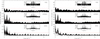 |
Fig. 9 As in Fig. 8 but for the Hα line. |
| In the text | |
|
Fig. 10 Multiplied Scargle periodograms (top panels) of all three individual FIES, HERMES, and SONG datasets, after rescaling each one of them to their dominant frequency (see text), compared with the periodogram of the merged dataset (bottom panels) for the first moment of the Si III λ4552 (left) and Hα (right) lines.Thick dashed lines indicate some of the dominant frequencies identified in any of the four periodograms. Thin dotted lines show their ±1 day aliases. |
| In the text | |
|
Fig. 11 Scargle periodograms of the first moment of the Si III λ4552 line from several of the HERMES and SONG individual runs (see Table 1) and the complete dataset (bottom panel, see notes in Fig. 10). |
| In the text | |
|
Fig. 12 Line profiles averaged over 16 individual consecutive measurements of the SONG spectroscopy of the first (black) and second (red) intensive campaigns. The top two panels are for photospheric lines (left: Si III, right: O II) while the bottom two panels are for lines affected by the stellar wind (left: He I with sharp dips caused by telluric lines, right: Hβ ). |
| In the text | |
|
Fig. 13 Temporal distribution of residuals in λ-space for three representative line profiles in HD 2905. (Left) Si III λ4567 as an example of a purely photospheric line. (Right) Hα as the most extreme case of optical line affected by stellar wind. (Middle) Hβ as an intermediate case. We also include for reference purposes three sinusoidal curves with associated frequencies 0.055 d−1 (pink), 0.019d−1 (blue), and 0.369 d−1 (purple), respectively (see Sect. 4.2.3 for discussion). Panels to the left show the temporal variation of the centroid of each line-profile (⟨v⟩). Bottom panels include several individual profiles corresponding to the dates indicated as horizontal lines in the left panels, as well as the mean profile obtained from the complete FIES+HERMES+SONG spectroscopic dataset. |
| In the text | |
Current usage metrics show cumulative count of Article Views (full-text article views including HTML views, PDF and ePub downloads, according to the available data) and Abstracts Views on Vision4Press platform.
Data correspond to usage on the plateform after 2015. The current usage metrics is available 48-96 hours after online publication and is updated daily on week days.
Initial download of the metrics may take a while.