| Issue |
A&A
Volume 611, March 2018
|
|
|---|---|---|
| Article Number | A5 | |
| Number of page(s) | 27 | |
| Section | Interstellar and circumstellar matter | |
| DOI | https://doi.org/10.1051/0004-6361/201731814 | |
| Published online | 13 March 2018 | |
Large Interstellar Polarisation Survey
II. UV/optical study of cloud-to-cloud variations of dust in the diffuse ISM
1
European Southern Observatory,
Karl-Schwarzschild-Str. 2,
85748
Garching b. München,
Germany
e-mail: This email address is being protected from spambots. You need JavaScript enabled to view it.
2
Sobolev Astronomical Institute, St. Petersburg University,
Universitetskii prosp. 28,
198504
St. Petersburg,
Russia
3
Armagh Observatory and Planetarium,
College Hill,
Armagh BT61 9DG,
UK
4
Anton Pannekoek Institute for Astronomy, University of Amsterdam,
1090
GE Amsterdam,
The Netherlands
5
Department of Physics and Astronomy and Centre for Planetary Science and Exploration (CPSX), The University of Western Ontario,
London,
ON N6A 3K7,
Canada
6
SETI Institute,
189 Bernardo Ave, Suite 100,
Mountain View,
CA
94043,
USA
7
ACRI-ST, 260 route du Pin Montard,
06904,
Sophia Antipolis,
France
Received:
22
August
2017
Accepted:
23
November
2017
Abstract
It is well known that the dust properties of the diffuse interstellar medium exhibit variations towards different sight-lines on a large scale. We have investigated the variability of the dust characteristics on a small scale, and from cloud-to-cloud. We use low-resolution spectro-polarimetric data obtained in the context of the Large Interstellar Polarisation Survey (LIPS) towards 59 sight-lines in the Southern Hemisphere, and we fit these data using a dust model composed of silicate and carbon particles with sizes from the molecular to the sub-micrometre domain. Large (≥6 nm) silicates of prolate shape account for the observed polarisation. For 32 sight-lines we complement our data set with UVES archive high-resolution spectra, which enable us to establish the presence of single-cloud or multiple-clouds towards individual sight-lines. We find that the majority of these 35 sight-lines intersect two or more clouds, while eight of them are dominated by a single absorbing cloud. We confirm several correlations between extinction and parameters of the Serkowski law with dust parameters, but we also find previously undetected correlations between these parameters that are valid only in single-cloud sight-lines. We find that interstellar polarisation from multiple-clouds is smaller than from single-cloud sight-lines, showing that the presence of a second or more clouds depolarises the incoming radiation. We find large variations of the dust characteristics from cloud-to-cloud. However, when we average a sufficiently large number of clouds in single-cloud or multiple-cloud sight-lines, we always retrieve similar mean dust parameters. The typical dust abundances of the single-cloud cases are [C]/[H] = 92 ppm and [Si]/[H] = 20 ppm.
Key words: dust, extinction / polarization / ISM: clouds / ISM: abundances
© ESO 2018
1 Introduction
In the transition regions between the diffuse and dense interstellar medium (ISM) of the Milky Way, large variations of the dust properties are observed (Chini & Kruegel 1983). These variations are theoretically explained by the fact that dust coagulation and accretion depend on the ambient density (Köhler et al. 2012). However, one does not expect variations of dust properties within the diffuse ISM, and the Milky Way is often assumed to be characterised by a “standard” extinction curve, which is due to a “typical dust mixture” in the diffuse ISM. This standard extinction curve is represented by a constant total-to-selective extinction ratio of RV ~ 3.1 (Morgan et al. 1953; Cardelli et al. 1989), and is widely applied for purposes of de-reddening and foreground removal.
There is observational evidence that the extinction curves of the diffuse ISM change from sight-line to sight-line (Fitzpatrick & Massa 1990, 2007). Such variations can be interpreted in terms of changes of the chemical composition and sizes of the grains, and of the various chemical and physical processes that are altering the dust. The distribution of RV in a local volume of the diffuse ISM reveals variations of dust properties on scales larger than individual clouds (Schlafly et al. 2017). By observing the spectral variation and spatial morphology of dust extinction curves in the Milky Way one may reveal the nature of the processes that are responsible for the variation of the dust properties in such local environments, and ultimately may help to understand the evolution of the dust in the Milky Way.
Variations of dust properties in the diffuse ISM have also been detected at large scales in the far infrared (IR) by the Planck Collaboration (Planck Collaboration XVII 2014; Planck Collaboration XXIV 2011; Planck Collaboration XXIX 2016). Bot et al. (2009) found that in the regions of cirrus clouds where the 60 μm/100 μm flux ratio decreases, the 160 μm/100 μm flux ratio increases. These colour variations cannot be explained by changing the interstellar radiation field (ISRF, Mathis et al. 1983), but are due to significant changes of the dust properties such as their size distribution, grain emissivity or mixing of clouds in different physical conditions. Understanding such variations is important also for an accurate removal of foreground contamination in extra-galactic studies.
Planck Collaboration XXIX (2016) found that in certain regions of the diffuse ISM, dust extinction decreases, temperature increases, but the luminosity per H atom is constant. A decrease of the dust extinction and increase of dust temperature could be explained by a change of the strength of the ISRF, but this would produce also a change in the luminosity, which is not observed. Therefore, a change of the dust properties has been suggested as an explanation. Recently, Ysard et al. (2015), who applied the Jones et al. (2013) dust model, could demonstrate that the Planck observation of the diffuse ISM dust emission Iν from 100−850 μm may be fit by  , where
  is the optical depth at ν0 = 353 GHz (850 μm), T is the dust colour temperature, and β is the submillimeter slope.
In this paper we present new information that support the hypothesis that dust properties are varying within the diffuse ISM and at small scales from cloud-to-cloud. We use the data of our recent spectro-polarimetric survey of the interstellar medium (Bagnulo et al. 2017), combined with data from the literature which provide extinction measurements (Sect. 2). For those stars for which high-resolution spectroscopic data are available in astronomical archives, we can disentangle sight-lines with a single-cloud from sight-lines with multiple component dust clouds. We then consider the former data set, and we apply the Siebenmorgen et al. (2014) dust model to fit simultaneously the extinction and polarisation curve (Sect. 3). By using the derived dust parameters towards individual sources of the Large Interstellar Polarisation Survey (LIPS, Sect. 4) we successfully search for correlations between dust and extinction or polarisation parameters when either single or multiple-cloud sight-lines are considered (Sect. 4). Finally, in Sect. 5 we summarise our main findings.
2 Observational data
We consider the targets observed with FORS2 in spectropolarimetric mode (see Sect. 2.1 below) for which there exist also measurements of the extinction curve (Sect. 2.2). This subsample includes 59 sight-lines. For this subsample we also searched in the ESO archive high-resolution UVES spectra (Sect. 2.3), which may be used to distinguish single-cloud from multiple-cloud sight-lines.
2.1 Spectro-polarimetry
To study the properties of interstellar dust in the diffuse ISM, we have recently obtained spectro-polarimetry data of a large sample of more than one hundred early-type OB stars in both hemispheres, using the FORS2 instrument (Appenzeller et al. 1998) of the ESO VLT for the Southern Hemisphere, and the ISIS instrument of the William Herschel Telescope for the survey in the Northern Hemisphere. The targets of this Large Intestellar Polarisation Survey (LIPS) are not associated to clouds and are widely distributed in the galactic disk, except for the two high galactic lattitude stars HD 203532 and HD 210121. In this paper we use the polarisation-spectra published by Bagnulo et al. (2017) in the context of the Southern part of LIPS, which includes 101 targets observed in the wavelength range 380–950 nm at a resolving power of λ∕Δλ ~ 880. For the targets with maximum polarisation higher than 0.7%, (76 out of 101), Bagnulo et al. (2017) report the best-fit parameters obtained using the empirical formula given by Serkowski et al. (1975)
![Mathematical equation: \begin{equation*}{p(\lambda)} = {p_{\max}} \ \exp \left[ -k_{\textrm{p}} \ \ln^2 \left( \frac{\lambda_{\max}}{\lambda} \right) \right],\end{equation*}](/articles/aa/full_html/2018/03/aa31814-17/aa31814-17-eq3.png) (1)
(1)
which includes three free parameters: the maximum polarisation pmax, the wavelength λmax at pmax, and the width of the spectrum kp.
2.2 Extinction
For 59 sight-lines of the LIPS targets observed by Bagnulo et al. (2017) we have retrieved the extinction curves in the range 2 μm–90 nm using the sample assembled by Valencic et al. (2004) and Gordon et al. (2009). These common sight-lines will be hereafter referred to as the LIPS sample. The dust extinction is derived using the so-called standard pair method (Stecher 1965), i.e., by measuring the ratio of the fluxes of pairs of reddened and unreddened stars with the same spectral type. With this method, the accuracy of the dust extinction estimate depends critically on how well the distance to the star is known. Unfortunately, distances to hot, early-type stars are subject to large errors; therefore one often prefers to rely on relative measurements by considering the extinction curve normalised to the value of the extinction in the V band. The extinction curve τ∕τV is then usuallyreproduced by a third-order polynomial and a Drude profile, which accounts for the 217 nm extinction bump. Fitzpatrick & Massa (1990, 2007); Valencic et al. (2004); Gordon et al. (2009) express the extinction curve in the range x = 1∕λ ≥ 3.3 μm−1 by:
 (2)
(2)
where F(x), which describes the non-linear UV part of the curve, is defined as

and D(x, γ, x0) is the Drude profile
 (3)
(3)
with damping constant γ and central wavelength 1∕x0. We note that for 75 sight-lines, Gordon et al. (2009) have refined the extinction parametrisation by supplementing data from the International Ultraviolet Explorer (IUE) at 3.3 μm−1 < λ−1 < 8.6 μm−1 with Far Ultraviolet Spectroscopic Explorer (FUSE) spectra at 3.3 μm−1 < λ−1 < 11 μm−1. Following their work, we adopt for the c4 coefficient a value which is ~8% smaller thanthat estimated from the IUE data alone by Valencic et al. (2004) for stars with no available FUSE data. At longer wavelengths, specifically for the UBV JHK bands, we apply the RV parametrisation presented by Fitzpatrick (2004), where RV = AV∕E(B − V) is the ratio of total-to-selective extinction.
2.3 Optical high-resolution spectra
We retrievedUVES high-resolution spectra (λ∕Δλ ~ 105) from the ESO archive for 32 of the LIPS sample stars. UVES (Dekker et al 2000) is an instrument that provides spectra in the range 300–1100 nm with a spectral resolution up to 110 000. For this project, we were primarily interested in the profiles and shapes of interstellar absorption lines arising from the diffuse ISM, such as the K and H component of Ca II at 393.366 and 396.847 nm1; of the Na I doublet at 330.237 and 330.298 nm; and the K I line at 769.9 nm. Velocity profiles of Ca II are usually more complex than those of neutral species (Na I, K I). The former traces warmer, more widespread ISM, while the latter lines probe colder regions (Pan et al. 2005).
We followed the method proposed by Krełowski (2014) and Sonnentrucker et al. (1999), which is also applied to studies of diffuse interstellar bands (Cami et al. 1997; Ensor et al. 2017): we measured the radial velocities from various spectral lines in the line of sight toward a given target. If all radial velocities are identical, it means that the star is observed through just a single-cloud; if instead the interstellar lines are broadened or split in multiple redor blue Doppler shifted velocity components, then between us and the target star there must be two or more interstellar clouds. Finally we assume that the gas and dust in the diffuse ISM is well-mixed, so that the gas distribution traced by the atomic lines is a good proxy of the dust distribution. In total, we found suitable UVES spectra for 32 stars in our LIPS sample that display one or more interstellar absorption lines of Ca II, Na I, and K I; the currently ongoing EDIBLES program (Cox et al. 2017) will result in more good candidates in the near future. We report our results in Table 1, where we distinguish the lines into single (“S”), dominated by a single (“dS”), and multiple component (“M”) profiles. Our analysis of UVES spectra confirm the result previously found by Krełowski (2014) that the vast majority of reddened OB stars are observed through two or moreinterstellar clouds. However, we found that eight out of the 59 LIPS sight-lines are crossing just a single absorbing dust cloud. Figure 1 shows the UVES spectra of these eight stars observed through a single-cloud sight-line. These stars will be subject to our special analysis in Sect. 4.
Intersections of clouds towards targets.
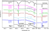 |
Fig. 1 Relative intensities of UVES spectra in the Na I, Ca II H, Ca II K and K I absorption lines for sight-lines with a single-cloud in the observing beam. |
3 Dust model
To fit the wavelength-dependence of extinction and linear polarisation of the LIPS sample, we used the dust model from Siebenmorgen et al. (2014) in which silicate and carbonaceous dust particles are considered. Extinction data cannot be reproduced by grains with a single size, therefore we adopted the well-known power-law size distribution n(r) ∝ r−q (the so-called MRN distribution; see Mathis et al. 1977) in addition to polycyclic aromatic hydrocarbon molecules (PAHs) with 150 C atoms and 60 H atoms. Significant contributors to the extinction are small silicates (sSi) in the far-UV, small graphite (gr) and PAH in the 217.5 nm extinction bump region, large amorphous carbon (aC) with a nearly constant extinction at 2 ≤ x = 1∕λ ≤ 7 μm−1, and large silicates (Si) that show a linear increase of the extinction with x in that range.
Draine & Hensley (2016) pointed out that the rapid fall-off of the polarisation of starlight in the far-UV suggests that small (r < 6 nm) grains are nearly spherical and do not contribute to the far-UV polarisation. On the other hand, interstellar polarisation cannot be explained by spherical particles made of optically isotropic material. There must be large, partly aligned, and non-spherical grains. We consider spheroids as simple examples. They come in two flavours: prolates, which are obtained by a rotation of an ellipse around the major axis a (e.g. like a rugbyball); or oblates, which are obtained by a rotation of an ellipse around the minor axis b (i.e. more disk-like). Unless the degree of the polarisation is very high, prolates provide better fits to polarisation spectra than oblates (Voshchinnikov & Hirashita 2014; Siebenmorgen et al. 2014; Voshchinnikov et al. 2016). We use prolates with a∕b = 2; their volume is the same of a sphere with radius  . Following Hirashita & Voshchinnikov (2014) we employ different upper size limits
  and
and  for large amorphous carbon and silicate grains.
To compute the scattering and absorption efficiencies of the spheroidal dust grains we have used a solution to the light scattering problem given by Voshchinnikov & Farafonov (1993). We have computed cross-sections of prolate aC and Si particles for 100 values of their radius, in the interval from 6 to 800 nm. For aC grains, we have adopted optical constants of the ACH2 hydrogenated amorphous carbon particle mixture by Zubko et al. (1996) with bulk density of 1.6 g cm−3 (Furton et al. 1999; Robertson 1996; Casiraghi et al. 2005). For silicates, we have considered optical constants by Draine (2003) and a density of 3.5 g cm−3. Formulas for computing the various extinction and polarisation cross sections Kext and Kp are given by Siebenmorgen et al. (2014). The extinction curve for each star is fit by
 (4)
(4)
where Kext is the extinction cross section of the dust averaged over sizes and rotations in units cm2 ∕g-ISM dust. Distances of our sample stars are small enough (generally <~1 kpc) so that systematic uncertainties due to incoherent scattering can be ignored (Scicluna & Siebenmorgen 2015). The observed linear polarisation is fit by
 (5)
(5)
where Kp is the linearpolarisation cross section of aligned silicates averaged over sizes and rotations in units cm2 ∕g-ISM dust. We do not need to consider alignment of carbon particles when fitting the data. The polarisation strength depends critically on the axial ratio of the spheroids a∕b, the alignment efficiency δ0 of the assumed imperfect Davis–Greenstein alignment, and the magnetic field orientation Ω. However, none of these parameters have a significant impact on the spectral shape of the polarization curve (Voshchinnikov 2012; Siebenmorgen et al. 2014; Voshchinnikov et al. 2016). Therefore we can simplify our modeling efforts and do not fit the absolute value of pmax. We scale the polarisation spectrum of the dust model to the data using pmax /Kp(λmax) as scaling parameter (Eq. (5)). We apply the same choice of parameters as in Siebenmorgen et al. (2014), namely prolate spheroids with axial ratio a∕b = 2, δ0 = 10 μm, and Ω = 90o. We need to introduce a minimum radius of aligned silicate  when fittinga polarisation curve (Draine & Fraisse 2009; Das et al. 2010).
For each dust component, its specific mass (or its relative abundance) needs to be specified. Scaling these abundances up or down by a constant factor does not change the predicted extinction or polarisation curve. For direct comparison with cosmic abundance constraints (Draine 2011) we set as normalisation [Si]/[H] = 15 ppm in large silicate grains, which is at the low end of 15 ≤ [Si]∕[H] ≤ 31.4 (ppm) reported by Voshchinnikov & Henning (2010). The rest of Si is locked up in small silicates.
The amount of [C]/[H] depleted in dust is difficult to estimate and there are various numbers in the literature. The interstellar absorption feature at 3.4 μm can be explained by hydrogenated amorphous carbon with 72 ≤ [C]∕[H] ≤ 97 (ppm) (Duley et al. 1998; Furton et al. 1999), when using a gas phase abundance by Sofia et al. (2004) [C]∕[H] = 84 ± 23 ppm is estimated by Nieva & Przybilla (2012), for the same reference abundance a median [C]∕[H] = 102 ± 47 ppm is derived by Parvathi et al. (2012), and assuming that half of C is depleted into grains [C]/[H] as low as 25 ≤ [C]∕[H] ≤ 120 (ppm) is found by Gerin et al. (2015). We will see below that the carbon abundance used in the dust models is in good agreement with such estimates.
In addition depletion of Fe and O on dust is openly discussed (Dwek 2016; Jenkins 2009; Köhler et al. 2014) as well as the details of the silicate mineralogy (Henning 2010).
4 Results
We fit extinction and polarisation spectra of the LIPS sample applying the procedure described by Siebenmorgen et al. (2017), which is based on a minimum χ2 technique utilizing the Levenberg–Marquardt algorithm as implemented in MPFIT2 (Markwardt 2009). In the χ2-fit the extinction and polarisation data are treated with the same weight.
There are in total eight free parameters: four size parameters q,  ,
,  ,
,  , and one abundance for each dust component: [C]/[H]aC, [C]/[H]gr, [C]/[H]PAH, [Si]/[H]sSi, we remind that our normalisation is [Si]/[H]Si = 15 ppm. The abundance is converted into weight or specific mass wi = mi of each dust component i as in Eq. (15) by Siebenmorgen et al. (2014). We included a slight improvement in the fitting procedure by adjusting the center wavelength of the Drude profile of the PAH cross section in the 217.5 nm bump region to the observed extinction peak. The best-fit parameters with 1σ uncertainties are listed in Table 2. Figure 2 shows the best-fit to the extinction curves for the single-cloud sight-lines, together with the contributions of the different dust populations, and Fig. 3 shows the corresponding fits to the polarisation curves. The best-fits of the other cases are shown in the appendix. In the following we discuss the cloud-to-cloud variations of the dust parameters and correlations of the dust parameters with observing characteristics for extinction c1, c2, c3, c4, RV, and polarisation kp, λmax, and pmax. We will see that generally the extinction and polarisation curve of the LIPS sources are well fit by the dust model, that the abundances in the dust model are consistent with present cosmic abundance constraints, and that single-cloud sight-lines show correlations that are not present in multiple-cloud cases.
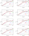 |
Fig. 2 Observed and modeled extinction curve of single-cloud sight-lines. The extinction curve by Fitzpatrick (2004), Valencic et al. (2004) and Gordon et al. (2009) is shown as dashed line, UBV JHK photometry as filled circles, IUE/FUSE spectra are represented by the grey shaded area, and uncertainties are 1σ. The model is shown (brown solid lines), as well as the contribution of the different dust populations to the extinction (solid lines of various colours as labelled in the panels). |
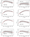 |
Fig. 3 Polarisation curves of single-cloud sight-lines. The polarisation spectra obtained with FORS2 are shown with grey lines; the filled circles (with 1σ error bars) show the same data rebinned to a spectral resolution of λ∕Δλ ~ 50. The best-fit obtained with our dust model is shown with a brown solid line. |
4.1 Parameter study
The distribution of the best-fit parameters are displayed in Fig. 4 for the stars of the LIPS sample (grey) and the single-cloud sight-lines (red). Single-cloud sight-lines have median values with 1σ variations of the dust abundances of [C]/[H]tot = 94 ± 10 ppm and [Si]/[H]tot = 20 ± 2 ppm (Table 2). They are in good agreement with the above estimates of the cosmic abundances in dust. For some individual sources there are noticeable outliers. Examples are the translucent sight-line towards HD 147888 in the ρ Orph complex and HD 37021 in the Orion nebulae. For HD 147888 Voshchinnikov & Henning (2010) finds a total [Si]/[H] = 30 ± 1.5 ppm in dust. Applying this value increases [C]/[H]tot to 169 ppm, in dust which would equal the gas phase abundance of [C]/[H]gas = 169 ± 38 ppm derived by Sofia et al. (2004). For HD 37021 we derive [C]/[H]tot = 211 ± 18 ppm and this value would even double when applying [Si]/[H]tot = 30 ± 1.5 ppm (Voshchinnikov & Henning 2010). It is certainly above the available C abundance as estimated by Sofia et al. (2004). Strikingly the latter authors find RV = 4.6 while we apply RV = 5.84 following Valencic et al. (2004). Extinction curves for both stars are displayed in Figs. 2 and A.5. For the [C]/[Si] abundance ratio we find a lower bound of 3.9 as derived towards HD 45314 (Table 2).
We find for single-cloud sight-lines typical size parameters of q = 3.0 ± 0.4,  nm,
nm,  nm, and
  nm (Table 2). By considering the full sample one finds parameter distributions that are wider but within 1σ similar median values, e.g.
  nm (Fig. 4). Sizes of large silicates are further constrained by the polarisation spectra so that one finds a somewhat larger scatter in the upper limit to the aC grain size
  .
.
We remove from our LIPS sample all known single-clouds cases (eight), and consider in total 51 stars. This new subsample, will be called hereafter “L-sample”. It includes all multiple-clouds cases, plus six cases which we cannot determine if they are single or multiple sight-lines. For these 51 sight-lines we verify if their average dust properties differ from the eight single-cloud cases. To perform this check, we have taken 105 random samples of 8stars selected out of these 51 stars. For each of these elements we have computed the median of the best-fit parameters. We find within 1σ the same median dust properties as computed for the LIPS sample. By attempting to find average dust properties similar values are derived for single- or multiple-cloud sight-lines. Such average dust properties will be always observed either by mixing of several clouds in single-cloud sight-lines or by mixing of clouds in multiple-cloud sight-lines. Exceptions are the abundances of the small grains and the upper grain size of carbon dust  , which are also the parameters affected by the largest errors. Note the large cloud-to-cloud variations in each of the dust parameters when comparing individual cases (Fig. 4).
Finally, we checked how the estimate of dust parameters change if we neglect the constraint from polarimetric measurements. Figure 5 shows the histograms of q and mean sizes of large silicates  and amorphous carbon
  . Mean sizes are computed by averaging over the dust size distribution from 6 nm to r+. Histograms are shown for these parameters when each target of the LIPS sample is either simultaneously fitting the extinction and polarisation curve (red) or the extinction curve only (grey). The median of the dust parameters when fitting extinction and polarisation are q = 3.0 ± 0.4,
  nm, and
  nm, and when fitting extinction only q = 2.4 ± 0.4,
  nm, and
  nm. By deriving dust properties only from extinction and ignoring polarisation measurements, one retrieves a flatter dust size distribution and larger mean grain sizes than when polarimetric measurements are included in the analysis.
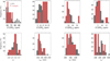 |
Fig. 4 Histograms of best-fit parameters for all stars of the LIPS sample (shaded area in grey) and the single-cloud sight-lines (shaded area in red). The intersection of both samples is shownas red-grey hatched area. In the top panels we show (from left to right) the dust abundances [C]/[H]aC, [C]/[H]gr, [C]/[H]PAH, and [Si]/[H]sSi, and in the bottom panels q, |


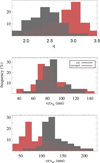 |
Fig. 5 Histograms of the exponent of the size distribution (top) and mean sizes of silicates (middle) and amorphous carbon (bottom) forthe LIPS sample when fitting extinction and polarisation (shaded area in red) and extinction only (shaded area in grey). The intersection of both samples is shown as grey-red hatched area. |
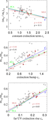 |
Fig. 6 Top panel: mass ratio of silicate and carbon dust versus the constant term c1 of Eq. (2) in observations of the extinction curve between 115–330 nm (Valencic et al. 2004; Gordon et al. 2009). Mid panel: mass ratio of very small (r < 6 nm) and large grains versus the parameter c3 of Eq. (2); the parameter c3 describes the strength of the extinction bump. Bottom panel: mass ratio of very small (r < 6 nm) and large grains versus the parameter c4 of Eq. (2), which describes the strength of the far UV rise. The L-sample is shown with open circles and the LS -sample with grey filled circles together with their Pearson coefficient (black). Single-cloud sight-lines (red squares) with 1σ error bars and Pearson coefficient are shown in red. They are fit by straight lines employing the MLE (red solid line), PCA (green solid line), and minimum χ2 (blue solid line) method. |
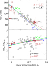 |
Fig. 7 Mean radius of large silicate grains (top) and mass ratio of silicate and carbon (bottom) versus extinction fit parameter c2. The c2 parameter describes a linear term in observations of the extinction curve between 115–330 nm (Valencic et al. 2004; Gordon et al. 2009). The dashed lines are straight-line fits of data belonging to the LS -sample (filled circles in grey) and full lines are fits to the single-cloud sight-lines. Symbols same as in Fig. 6. |
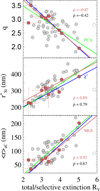 |
Fig. 8 Exponent of the dust size distribution (top), upper radius of large silicates (middle)and mean radius of large carbon grains (bottom) versus total-to-selective extinction RV. Symbols same as in Fig. 6. |
 |
Fig. 9 Mean radius of large silicate grains versus wavelength at maximum polarisation (top). Minimum radius of aligned silicates versus width of the polarisation spectrum (bottom). Symbols as in Fig. 6. |
4.2 Correlation study
As a first step for a physical interpretation of the observations we searched for relations between the dust model parameters and the observing characteristics for extinction c1, c2, c3, c4, RV, and polarisation kp, λmax. The linear Pearson correlation coefficient − 1 ≤ ρ ≤ 1 can be taken as a measure of the correlation strength. We assume that for |ρ| > ~ 0.8 a correlation could exist that we further investigate by other means. The existence of a trend in both data is tested by employing three different straight-line fits y = a ⋅ x + b, where 1σ errors (Δx, Δy) in both coordinates(x, y) are considered (for a discussion of issues concerning straight-line fits see Hogg et al. 2010). A first and most common applied treatment is the minimum χ2 technique called fitexy by Press et al. (1992). A second procedure is a principal component analysis (PCA). In PCA one computes eigenvectors and eigenvalues of the covariance matrix. The eigenvalues are renormalised so that their sum equals 1. The eigenvector that belongs to the renormalised eigenvalue with the highest value is taken as the principal component and provides our fit parameters a, b. We include in PCA the measurement uncertainties by drawing 10 000 random samples that are consistent with the 1σ error of the data and assuming Gaussian noise distribution. For each of such samples we perform a PCA and derive the probability density function (PDF) of a and b. We are most interested in the slope of the potential correlation so that we take the value of a where its distribution function peaks, and take thecorresponding value of b. Finally, we apply the Bayesian maximum likelihood estimator (MLE) as provided by Kelly (2007). The later provides also the PDF of the fitting parameters. The range where 68% of the parameter is scattered around its peak of the PDF is quoted as uncertainty. MLE outperforms the χ2 and PCA estimators whenever the measurement uncertainties are not strictly Gaussian functions (Hogg et al. 2010). For low values of |ρ| the slope parameters a derived by the χ2, PCA, and MLE might become arbitrary, while for |ρ|> ~ 0.8 more consistent slopes are found. We consider that a correlation exists when all three regression estimators provide a similar trend in the data. It is then still important to consider the issue of outliers. Random samples that include a single extreme value in the abscissa result in high |ρ| values. Such extreme data are better removed in the correlation study.
We compare correlations of single-cloud sight-lines with different samples of multiple-cloud (dominated) sight-lines. We recall that we have defined as S-sample the eight LIPS targets observed through single-cloud sight-lines, as identified through UVES data. The 24 multiple-cloud sight-lines as identified thanks to UVES data represent the M-sample. The complete 59 LIPS objects excluding the eight stars of the S-sample (51 multiple-cloud dominated sight-lines) is called L-sample. For a proper comparison of the correlations, we will also consider the targets from M-sample that have ci and RV parameters in the same range as the stars of the S-sample. By so-doing, we have selected a sub-subsample of multiple-cloud sight-lines that we call MS. We do the same kind of selection for the L-sample, and we define the LS sample as the list of LIPS targets that are not identified as single-clouds sight-lines, but that have parameters ci and RV in the same range as the S-sample stars. In the observed extinction characteristics, the M-sample has a narrower range than the S-sample. For example, the M-sample is observed between 0.87 ≤ c1 ≤ 1.6 and 2.8 ≤ RV ≤ 4.9, whereas the S-sample is between 0.75 ≤ c1 ≤ 2.3 and 2.3 ≤ RV ≤ 5. Finally, we consider further sub-samples of MS and LS, by considering the stars for which the ratios pmax∕AV and either kp or λmax are in the same range as the stars of the S-sample. We will call these subsamples MSP and LSP.
Pearson’s correlation coefficients ρ between dust model and extinction or Serkowski parameters are given for the single-cloud and the other samples in Tables 3 and 4. The high latitude star HD 210121 has peculiar far UV extinction (Weingartner & Draine 2001) with extreme values in the extinction parameters. Therefore it is excluded from the S-sample, except for the correlation study with RV, where HD 210121 has a normal behaviour. For large |ρ| we show data in Figs. 6–9. Data considered in the correlation study are marked by filled symbols. Samples with the strongest |ρ| are fit by the χ2, PCA, and MLE method. In Table 5 we report straight-line parameters derived by MLE with error estimates and confidence that the fit is not due to selection bias (Sect. 4.3).
Pearsons’ correlation coefficient between dust model and the extinction curve parameters c1, c2, c3, c4 of Eq. (2) and RV for various LIPS sub-samples.
Pearsons’ correlation coefficient ρ between dust and Serkowski parameters kP, λmax of various LIPS sub-samples.
Regression fits between dust and observing parameters.
4.2.1 Model versus extinction parameters
In the rangex > ~ 3 μm−1, the extinction curve is described by Eq. (2), which contains a constant term c1 and and a linear term with coefficient c2. In our dust model, this behaviour of the extinction curve depends on the mass ratio of silicate to carbon grains  , i.e., on the chemical composition of the dust cloud. The higher the specific mass of silicate relative to carbonaceous dust, the smaller the constant c1, and the larger the coefficient ofthe linear term c2. Typical examples for extinction curves that are flat in the spectral range 6 ≤ x ≤ 8 μm−1 are HD 147889 and HD 164740 (Fig. 2). They show large values of c1 of 1.6 and 1.5, small values of c2 ≤ 0.03, and a mass ratio as low as
  . On the other hand, HD 79186 has a steep extinction in that spectral range (Fig. 2) with c1 = 1.1, c2 = 0.26, and with
  . The star has about the largest of mass ratio in our sample. We observe for single-cloud sight-lines a positive correlation of
  with c1 (Fig. 6) and a negative for c2 (Fig. 7, bottom). Both correlations vanish for the other samples of multiple-cloud (dominated) sight-lines. Apparently the correlations break down when observing through clouds with different chemical compositions. However, for single-cloud sight-lines there are only data available that are scattered near c2 ~ 0 and ~ 2.6 so that these correlations need further proof.
Large carbon grains have a flat contribution to the extinction in the range between 2 ≤ x ≤ 7 μm−1 whereas large silicate grains increase linearly with x. Examples are given in Fig. 2. We find that by increasing the mean size of silicates the linear extinction rise c2 is reduced. We observe that the anti-correlation of  with c2 is stronger for the M, L samples with ρ ~−0.9 than for the S sample having ρ ~−0.8 (Fig. 7, top). The weaker correlation is driven by the less well constrained
  parameter of HD 129557.
We find for single-cloud cases that the strength of the extinction bump c3 is correlated with the mass ratio of small to large grains mvsg∕mlrg (Fig. 6). For example (Table 2), the [C]/[H] abundance in PAH and small graphite is 12 ppm for HD 164740, which has c3 = 0.7; whereas much more (28 ppm) C is locked in small grains for HD 79186 having a larger c3 of 1.2. By observing a mix of clouds the mvsg∕mlrg correlation with c3 breaks (Fig. 6).
Extinction curves with a large value of c4 display a strong far-UV rise at x > ~ 5.9 μm−1 (Eq. (2)). We observe a bi-modal distribution with two single-cloud cases with a far-UV extinction as flat as c4 ~ 0.1 and five stars with a steep far-UV rise clustered near c4 = 0.25. In the models the far-UV extinction of the later 5 stars have a significant contribution by small grains (Fig. 2, Table 2). For example, the abundance ratio of very small to large grains is for HD 129557 almost a factor three larger than for the flat far-UV extinction observed towards HD 164740 (Table 2). Indeed, we observe that the c4 parameter is strongly correlated with the mass ratio of very small and large grains (Fig. 6). The correlation is very strong in the single-cloud cases (ρ = 0.94), strong in the L- and LS-samples (ρ = 0.85 − 0.89), and weak, if at all present, in the M-sample (ρ < 0.8).
In the Weingartner & Draine (2001) dust model, small grains coagulate onto large grains in relativelydense environments. The ratio of visual extinction to hydrogen column density AV ∕NH ∝ RV, and so one expects that an increase of RV goes hand in hand with an increase of the mean particle radius and a flatter size distribution. This was noted already by Kim et al. (1994) in which for RV = 5.3 their size distribution has significantly fewer grains with r < 0.1 μm than their RV = 3.1 distribution, as well as a modest increase at larger sizes. This result is expected, at short wavelengths the extinction is provided by small grains and for larger values of RV there is relatively less extinction at short wavelengths. We prove these early conclusions by our observations (Fig. 8), however we can do this only for single-cloud sight-lines and not for the multiple-cloud samples. There is some trend in a correlation of the mean size of large silicates with RV for all sub-samples. For the S sample the mean size of large carbon grains as well as the upper grain radius of silicates correlates strongly with RV, and the exponent of the size distributions is anti-correlated with RV (Fig. 8). Again, this is because low values of q provide a relative increase of large grains. For multiple-cloud samples the latter relation becomes random with ρ ~ −0.5. (Table 3).
4.2.2 Model versus polarisation parameters
We have investigated if the best-fit parameters of the Serkowski curves exhibit differences between the case of single-cloud and multiple-cloud sight-lines. We found that the mean values of λmax and kp are almost the same for the8 single-cloud and the 51 multiple-cloud dominated sight-lines. However, we noticed that single-cloud cases show on average higher polarisation than the multiple-cloud sight-lines observed towards a particular sight-line: the median polarisation of the single-cloud cases is p = 2.6% (S-sample), whereas multiple-cloud sight-lines (L-sample) show a median polarisation of p = 1.3%. Similar, the median polarisation per visual extinction is p∕AV = 1.8 for single and p∕AV = 0.8 (%/mag) for multiple-cloud sight-lines. The median polarisation per reddening is p∕E(B − V) = 5.8 for single and p∕E(B − V) = 3(%) for multiple-cloud sight-lines. Both S and L samples have similar median values for the visual extinction of AV = 1.5 and AV = 1.7 mag, and for the reddening ofE(B − V) = 0.50 and E(B − V) = 0.45 for the single-cloud and multiple-cloud sight-lines and have same median of RV ~ 3.4. Apparently photons are depolarised when they penetrate through different clouds, which is explained by cloud-to-cloud variations of the magnetic field direction and different grain alignment efficiency.
The influence of grain sizes and the minimum alignment radius,  , on the polarisation spectrum is discussed by Voshchinnikov et al. (2013) and Siebenmorgen et al. (2014). It is shown that the choice of
  and
and  is sensitive to the polarisation spectrum. Therefore one expects that these dust parameters are related to the Serkowski parameters λmax and kp. We also compute the mean size of aligned silicates
  , which is given by averaging over the dust size distribution from
  and
and  .
.
The parameters of the Serkowski curve and the dust parameters are strongly correlated in the single-cloud cases (ρ≳0.9), while no correlation is observed in the cases of multiple-cloud sight-lines, with two exceptions in the MSP-sample. However, the latter sample has a narrower observed parameter range than the S-sample so that this comparison needs to be taken with care. In Fig. 9 we show that kp is correlated with  and λmax is correlated with
  . The latter correlation has already been found by Chini & Kruegel (1983) and more recently by Voshchinnikov et al. (2016). Apparently depolarisation is active when multiple-clouds are in the sight-line so that these correlations vanish.
4.3 Observing bias
We wish to quantify a confidence level that the correlations are not drawn by random selection effects of the sight-lines or a bias in the observing sample. We estimate a confidence level by means of Monte Carlo and select 105 random samples of 7 stars out of the total of 51 multiple-cloud sight-lines. For each of these elements we compute the correlation strength as given by Pearsons’ coefficient ρ′. This allows computing the probability ζ of finding a random correlation that is larger or equals the observed strength ρ′ ≥∥ρ∥, where ρ is given in Tables 3 and 4. For example, we observe that our single-cloud sight-lines c1 is anti-correlated with mSi∕mC at strength ρ = −0.95 (Table 3). We find that out of 104 random samples of 7 multiple-cloud dominated sight-lines selected from Table 2 there are only eight cases that show a correlation strength ρ′≤−0.95, hence ζ = 8∕10 000. We are confident at a 1 − ζ = 99.9% level that this correlation is not drawn by a random selection and can only be found when single-cloud sight-lines are observed. However, when a correlation pre-exists in the LIPS sample such confidence level shall be small. This is true for example in the  correlation, as given in Table 5. Excluding the 8 known single-cloud cases from the 59 LIPS targets we find that for any random selection of 7 out of the 51 such sight-lines there is a fifty-fifty chance that mvsg∕mlrg is correlated with c4 at ρ≥ 0.9. This explains why it was already observed before (Desert et al. 1990), that a large amount of very small relative to large grains steepens thefar-UV rise.
5 Conclusion
For 59 diffuse ISM sight-lines of the LIPS targets observed in spectro-polarimetric mode by Bagnulo et al. (2017) we have retrieved from previous literature the extinction curves in the range 2 μm–90 nm. For this sample we have performed the simultaneous modelling of normalised extinction and polarisation curves using an interstellar dust model that includes a populations of carbon and silicate dust in form of nano-sized particles and large (>~6 nm) spheroidal grains with a power law size distribution and imperfect rotational orientation. Using archive spectroscopic observations of interstellar absorption lines (Ca II, Na I, and K I), we have found that eight sight-lines are crossing just a single absorbing interstellar cloud. We have performed the analysis of our results independently for single interstellar clouds and for multi-cloud sight-lines. The main results of our analysis can be summarised as follows.
- 1.
For the eight single-cloud sight-lines, the ratio of total-to-selective extinction RV correlates strongly with the mean size of large silicate and carbon grains and anti-correlates with the exponent q of the dust-grain size-distributions (as expected, since the relative amount of large grains is larger for smaller values of q).
- 2.
For single-cloud sight-lines we have revealed several strong correlations between the parameters ci of the UV extinction curve fitting (see Eq. (2)) and the dust model parameters. For example, the mass ratio of total silicate to carbon
 is anti–correlated with c1 and correlated with c2, and the mass ratio of very small to large grains mvsg∕mlgr is correlated with c3. These correlations disappear when instead of considering only the single-cloud sight-lines we include stars observed through multiple-clouds with different chemical compositions. However, some relations are strong in both the single-cloud sample and the full LIPS sample. For instance, the c4 parameter, which provides a measure of the strength of the far-UV rise, is strongly correlated with the amount of small to large grains, mvsg∕mlgr, as expected.
 - 3.
Polarimetry imposes additional constraints on the dust properties than those given by extinction data only; in particular, simultaneous modelling of extinction and polarisation gives a steeper dust-grain size-distributions and smaller mean grain sizes than what is deduced from extinction data only.
- 4.
The interpretation of polarisation data from multiple-clouds sight-lines is more complicated After the radiation is polarised in a dust cloud, the intersection of a second or more clouds towards the sight-line leads to depolarisation. This fact can be understood by cloud-to-cloud variations of the grain properties, dust alignment efficiency and the direction of the magnetic field.
- 5.
In the single-cloud cases we have found strong correlations between the parameters of the Serkowski curve and the silicate dust parameters. For example, the wavelength at which the polarisation reaches maximum λmax, correlates with the mean radius of aligned silicates
 , and the width of the polarisation spectrum kp with the minimum radius of aligned silicates
  . No dependencies of the Serkowski parameters on the mean radius of large carbon particles
  are found. This confirms conclusions of the previous modelling by Voshchinnikov & Hirashita (2014).
 - 6.
The strong correlationships between parameters found for single-cloud cases that are not seen in the full sample are statistically not likely to be due to selection bias in the LIPS sample. This is demonstrated by the fact that when one arbitrarily selects seven out of 51 stars of the, L-sample the dependencies are still not detected.
- 7.
Any mixing of clouds results in similar average dust model parameters, however there are strong variations of the dust properties and from cloud-to-cloud.
We demonstrated that only the framework of single-cloud analysis provides an unambiguous view of relations between dust properties and observables such as extinction and polarisation. The framework will help understanding the dust evolution from cloud-to-cloud and within their particular physical environments. We conclude that a most urgent task is to find more such single-cloud sight-lines and develop dust models for them.
Acknowledgements
We devote this paper to our good friend, close colleague and teacher, Dr. Nikolai V. Voshchinnikov, who suddenly passed away on December 17, 2017 at the age of 66. Nikolai continued a Russian tradition and dedicated his life to the study of light scattering problems. We will forever miss his deep theoretical understanding of cosmic dust and his clear way of explaining to us the intricacies of interstellar extinction and polarization. May he rest in peace. This research is based on data obtained from the ESO Science Archive Facility and in particula on observations collected under ESO programme 095.C-0855 and 096.C-0159 (PI=N.Cox). This research has also made use of the SIMBAD database, operated at the CDS, Strasbourg, France. We thank E. Krügel and J. Krełowski for interesting discussions and the referee V. Guillet for helping us to improve ourwork. NVV was partly supported by the RFBR grant 16-02-00194 and RFBR–DST grant 16-52-45005.
Appendix A Extinction and polarisation fits
Remaining extinction and polarisation fits of individual targets are displayed in Figs. A.1 to A.12.
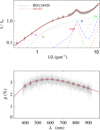 |
Fig. A.1 Top: observed and modeled extinction curve of BD 134920. The extinction curve by Fitzpatrick (2004), Valencic et al. (2004) and Gordon et al. (2009) is shown with a dashed line, UBV JHK photometrywith filled circles, IUE/FUSE spectra are represented by the grey shaded area, and uncertainties are 1 σ. The model is shown (brown solid line) as well as the contribution of the different dust populations to the extinction (various colored and labeled lines). Bottom: polarisation spectra observed with FORS2 are shown with grey lines, and the and best-fit model with brown solid lines; the filled circles (with 1 σ error bars) are the same data rebinned to a spectral resolution of λ∕Δλ ~ 50. |
References
- Appenzeller, I., Fricke, K., Fürtig, W., et al. 1998, The Messenger, 94, 1 [NASA ADS] [Google Scholar]
- Bagnulo, S., Cox, N. J. L., Cikota, A., et al. 2017, A&A, 608, A146 [NASA ADS] [CrossRef] [EDP Sciences] [Google Scholar]
- Bot, C., Helou, G., Boulanger, F., et al. 2009, ApJ, 695, 469 [NASA ADS] [CrossRef] [Google Scholar]
- Cami, J., Sonnentrucker, P., Ehrenfreund, P., & Foing, B. H. 1997, A&A, 326, 822 [NASA ADS] [Google Scholar]
- Cardelli, J. A., Clayton, G. C., & Mathis, J. S. 1989, ApJ, 345, 245 [NASA ADS] [CrossRef] [Google Scholar]
- Casiraghi, C., Ferrari, A. C., & Robertson, J. 2005, Phys. Rev. B, 72, 085401 [Google Scholar]
- Chini, R., & Kruegel, E. 1983, A&A, 117, 289 [NASA ADS] [Google Scholar]
- Cox, N. L. J., Cami, J., Farhang, A., et al. 2017, A&A, 606, A76 [NASA ADS] [CrossRef] [EDP Sciences] [Google Scholar]
- Das, H. K., Voshchinnikov, N. V., & Il’in, V. B. 2010, MNRAS, 404, 265 [NASA ADS] [Google Scholar]
- Desert, F.-X., Boulanger, F., & Puget, J. L. 1990, A&A, 237, 215 [NASA ADS] [Google Scholar]
- Draine, B. T. 2003, ApJ, 598, 1017 [NASA ADS] [CrossRef] [Google Scholar]
- Draine, B. T. 2011, Physics of the Interstellar and Intergalactic Medium (Princeton University Press) [Google Scholar]
- Draine, B. T., & Fraisse, A. A. 2009, ApJ, 696, 1 [NASA ADS] [CrossRef] [Google Scholar]
- Draine, B. T., & Hensley, B. S. 2016, ApJ, 831, 59 [NASA ADS] [CrossRef] [Google Scholar]
- Duley, W. W., Scott, A. D., Seahra, S., & Dadswell, G. 1998, ApJ, 503, L183 [NASA ADS] [CrossRef] [Google Scholar]
- Dwek, E. 2016, ApJ, 825, 136 [NASA ADS] [CrossRef] [Google Scholar]
- Ensor, T., Cami, J., Bhatt, N. H., & Soddu, A. 2017, ApJ, 836, 162 [NASA ADS] [CrossRef] [Google Scholar]
- Fitzpatrick, E. L. 2004, in Astrophysics of Dust, eds. A. N. Witt, G. C. Clayton, & B. T. Draine, ASP Conf. Ser., 309, 33 [NASA ADS] [Google Scholar]
- Fitzpatrick, E. L., & Massa, D. 1990, ApJS, 72, 163 [NASA ADS] [CrossRef] [Google Scholar]
- Fitzpatrick, E. L., & Massa, D. 2007, ApJ, 663, 320 [NASA ADS] [CrossRef] [EDP Sciences] [Google Scholar]
- Furton, D. G., Laiho, J. W., & Witt, A. N. 1999, ApJ, 526, 752 [CrossRef] [Google Scholar]
- Gerin, M., Ruaud, M., Goicoechea, J. R., et al. 2015, A&A, 573, A30 [NASA ADS] [CrossRef] [EDP Sciences] [Google Scholar]
- Gordon, K. D., Cartledge, S., & Clayton, G. C. 2009, ApJ, 705, 1320 [NASA ADS] [CrossRef] [Google Scholar]
- Henning, T. 2010, ARA&A, 48, 21 [NASA ADS] [CrossRef] [Google Scholar]
- Hirashita, H., & Voshchinnikov, N. V. 2014, MNRAS, 437, 1636 [NASA ADS] [CrossRef] [Google Scholar]
- Hogg, D. W., Bovy, J., & Lang, D. 2010, ArXiv e-prints [1008.4686] [Google Scholar]
- Jenkins, E. B. 2009, ApJ, 700, 1299 [NASA ADS] [CrossRef] [Google Scholar]
- Jones, A. P., Fanciullo, L., Köhler, M., et al. 2013, A&A, 558, A62 [NASA ADS] [CrossRef] [EDP Sciences] [Google Scholar]
- Kelly, B. C. 2007, ApJ, 665, 1489 [NASA ADS] [CrossRef] [Google Scholar]
- Kim, S.-H., Martin, P. G., & Hendry, P. D. 1994, ApJ, 422, 164 [NASA ADS] [CrossRef] [Google Scholar]
- Köhler, M., Stepnik, B., Jones, A. P., et al. 2012, A&A, 548, A61 [NASA ADS] [CrossRef] [EDP Sciences] [Google Scholar]
- Köhler, M., Jones, A., & Ysard, N. 2014, A&A, 565, L9 [NASA ADS] [CrossRef] [EDP Sciences] [Google Scholar]
- Krełowski, J. 2014, in The Diffuse Interstellar Bands, eds. J. Cami, & N. L. J. Cox, IAU Symp., 297, 23 [NASA ADS] [Google Scholar]
- Markwardt, C. B. 2009, in Astronomical Data Analysis Software and Systems XVIII, eds. D. A. Bohlender, D. Durand, & P. Dowler, ASP Conf. Ser., 411, 251 [NASA ADS] [Google Scholar]
- Mathis, J. S., Rumpl, W., & Nordsieck, K. H. 1977, ApJ, 217, 425 [NASA ADS] [CrossRef] [Google Scholar]
- Mathis, J. S., Mezger, P. G., & Panagia, N. 1983, A&A, 128, 212 [NASA ADS] [Google Scholar]
- Morgan, W. W., Harris, D. L., & Johnson, H. L. 1953, ApJ, 118, 92 [NASA ADS] [CrossRef] [Google Scholar]
- Nieva, M.-F., & Przybilla, N. 2012, A&A, 539, A143 [NASA ADS] [CrossRef] [EDP Sciences] [Google Scholar]
- Pan, K., Federman, S. R., Sheffer, Y., & Andersson, B.-G. 2005, ApJ, 633, 986 [NASA ADS] [CrossRef] [Google Scholar]
- Parvathi, V. S., Sofia, U. J., Murthy, J., & Babu, B. R. S. 2012, ApJ, 760, 36 [NASA ADS] [CrossRef] [Google Scholar]
- Planck Collaboration XXIV 2011, A&A, 536, A24 [Google Scholar]
- Planck Collaboration XVII 2014, A&A, 566, A55 [NASA ADS] [CrossRef] [EDP Sciences] [Google Scholar]
- Planck Collaboration XXIX 2016, A&A, 586, A132 [NASA ADS] [CrossRef] [EDP Sciences] [Google Scholar]
- Press, W. H., Teukolsky, S. A., Vetterling, W. T., & Flannery, B. P. 1992, Numerical recipes in FORTRAN, The art of scientific computing (Cambridge: University Press) [Google Scholar]
- Robertson, J. 1996, Phys. Rev. B, 53, 16302 [NASA ADS] [CrossRef] [Google Scholar]
- Schlafly, E. F., Peek, J. E. G., Finkbeiner, D. P., & Green, G. M. 2017, ApJ, 838, 36 [NASA ADS] [CrossRef] [Google Scholar]
- Scicluna, P., & Siebenmorgen, R. 2015, A&A, 584, A108 [NASA ADS] [CrossRef] [EDP Sciences] [Google Scholar]
- Serkowski, K., Mathewson, D. S., & Ford, V. L. 1975, ApJ, 196, 261 [NASA ADS] [CrossRef] [Google Scholar]
- Siebenmorgen,R., Voshchinnikov, N. V., & Bagnulo, S. 2014, A&A, 561, A82 [NASA ADS] [CrossRef] [EDP Sciences] [Google Scholar]
- Siebenmorgen,R., Voshchinnikov, N. V., Bagnulo, S., & Cox, N. L. J. 2017, Planetary and Space Science, 149, 64 [NASA ADS] [CrossRef] [Google Scholar]
- Sofia, U. J., Lauroesch, J. T., Meyer, D. M., & Cartledge, S. I. B. 2004, ApJ, 605, 272 [NASA ADS] [CrossRef] [Google Scholar]
- Sonnentrucker, P., Foing, B. H., Breitfellner, M., & Ehrenfreund, P. 1999, A&A, 346, 936 [NASA ADS] [Google Scholar]
- Stecher, T. P. 1965, ApJ, 142, 1683 [NASA ADS] [CrossRef] [Google Scholar]
- Valencic, L. A., Clayton, G. C., & Gordon, K. D. 2004, ApJ, 616, 912 [NASA ADS] [CrossRef] [Google Scholar]
- Voshchinnikov, N. V. 2012, J. Quant. Spec. Radiat. Transf., 113, 2334 [NASA ADS] [CrossRef] [Google Scholar]
- Voshchinnikov, N. V., & Farafonov, V. G. 1993, Ap&SS, 204, 19 [NASA ADS] [CrossRef] [Google Scholar]
- Voshchinnikov, N. V., & Henning, T. 2010, A&A, 517, A45 [NASA ADS] [CrossRef] [EDP Sciences] [Google Scholar]
- Voshchinnikov, N. V., & Hirashita, H. 2014, MNRAS, 445, 301 [NASA ADS] [CrossRef] [Google Scholar]
- Voshchinnikov, N. V., Das, H. K., Yakovlev, I. S., & Il’in, V. B. 2013, Astron. Lett., 39, 421 [NASA ADS] [CrossRef] [Google Scholar]
- Voshchinnikov, N. V., Il’in, V. B., & Das, H. K. 2016, MNRAS, 462, 2343 [NASA ADS] [CrossRef] [Google Scholar]
- Weingartner, J. C., & Draine, B. T. 2001, ApJ, 548, 296 [NASA ADS] [CrossRef] [Google Scholar]
- Ysard, N., Köhler, M., Jones, A., et al. 2015, A&A, 577, A110 [NASA ADS] [CrossRef] [EDP Sciences] [Google Scholar]
- Zubko, V. G., Mennella, V., Colangeli, L., & Bussoletti, E. 1996, MNRAS, 282, 1321 [NASA ADS] [CrossRef] [Google Scholar]
All wavelengths in air.
All Tables
Pearsons’ correlation coefficient between dust model and the extinction curve parameters c1, c2, c3, c4 of Eq. (2) and RV for various LIPS sub-samples.
Pearsons’ correlation coefficient ρ between dust and Serkowski parameters kP, λmax of various LIPS sub-samples.
All Figures
|
Fig. 1 Relative intensities of UVES spectra in the Na I, Ca II H, Ca II K and K I absorption lines for sight-lines with a single-cloud in the observing beam. |
| In the text | |
|
Fig. 2 Observed and modeled extinction curve of single-cloud sight-lines. The extinction curve by Fitzpatrick (2004), Valencic et al. (2004) and Gordon et al. (2009) is shown as dashed line, UBV JHK photometry as filled circles, IUE/FUSE spectra are represented by the grey shaded area, and uncertainties are 1σ. The model is shown (brown solid lines), as well as the contribution of the different dust populations to the extinction (solid lines of various colours as labelled in the panels). |
| In the text | |
|
Fig. 3 Polarisation curves of single-cloud sight-lines. The polarisation spectra obtained with FORS2 are shown with grey lines; the filled circles (with 1σ error bars) show the same data rebinned to a spectral resolution of λ∕Δλ ~ 50. The best-fit obtained with our dust model is shown with a brown solid line. |
| In the text | |
|
Fig. 4 Histograms of best-fit parameters for all stars of the LIPS sample (shaded area in grey) and the single-cloud sight-lines (shaded area in red). The intersection of both samples is shownas red-grey hatched area. In the top panels we show (from left to right) the dust abundances [C]/[H]aC, [C]/[H]gr, [C]/[H]PAH, and [Si]/[H]sSi, and in the bottom panels q, |
| In the text | |
|
Fig. 5 Histograms of the exponent of the size distribution (top) and mean sizes of silicates (middle) and amorphous carbon (bottom) forthe LIPS sample when fitting extinction and polarisation (shaded area in red) and extinction only (shaded area in grey). The intersection of both samples is shown as grey-red hatched area. |
| In the text | |
|
Fig. 6 Top panel: mass ratio of silicate and carbon dust versus the constant term c1 of Eq. (2) in observations of the extinction curve between 115–330 nm (Valencic et al. 2004; Gordon et al. 2009). Mid panel: mass ratio of very small (r < 6 nm) and large grains versus the parameter c3 of Eq. (2); the parameter c3 describes the strength of the extinction bump. Bottom panel: mass ratio of very small (r < 6 nm) and large grains versus the parameter c4 of Eq. (2), which describes the strength of the far UV rise. The L-sample is shown with open circles and the LS -sample with grey filled circles together with their Pearson coefficient (black). Single-cloud sight-lines (red squares) with 1σ error bars and Pearson coefficient are shown in red. They are fit by straight lines employing the MLE (red solid line), PCA (green solid line), and minimum χ2 (blue solid line) method. |
| In the text | |
|
Fig. 7 Mean radius of large silicate grains (top) and mass ratio of silicate and carbon (bottom) versus extinction fit parameter c2. The c2 parameter describes a linear term in observations of the extinction curve between 115–330 nm (Valencic et al. 2004; Gordon et al. 2009). The dashed lines are straight-line fits of data belonging to the LS -sample (filled circles in grey) and full lines are fits to the single-cloud sight-lines. Symbols same as in Fig. 6. |
| In the text | |
|
Fig. 8 Exponent of the dust size distribution (top), upper radius of large silicates (middle)and mean radius of large carbon grains (bottom) versus total-to-selective extinction RV. Symbols same as in Fig. 6. |
| In the text | |
|
Fig. 9 Mean radius of large silicate grains versus wavelength at maximum polarisation (top). Minimum radius of aligned silicates versus width of the polarisation spectrum (bottom). Symbols as in Fig. 6. |
| In the text | |
|
Fig. A.1 Top: observed and modeled extinction curve of BD 134920. The extinction curve by Fitzpatrick (2004), Valencic et al. (2004) and Gordon et al. (2009) is shown with a dashed line, UBV JHK photometrywith filled circles, IUE/FUSE spectra are represented by the grey shaded area, and uncertainties are 1 σ. The model is shown (brown solid line) as well as the contribution of the different dust populations to the extinction (various colored and labeled lines). Bottom: polarisation spectra observed with FORS2 are shown with grey lines, and the and best-fit model with brown solid lines; the filled circles (with 1 σ error bars) are the same data rebinned to a spectral resolution of λ∕Δλ ~ 50. |
| In the text | |
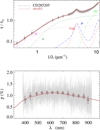 |
Fig. A.2 Notation same as in Fig. A.1 for CD 285205. |
| In the text | |
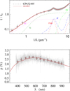 |
Fig. A.3 Notation same as in Fig. A.1 for CP 632495. |
| In the text | |
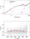 |
Fig. A.4 Notation same as in Fig. A.1 for HD 36982. |
| In the text | |
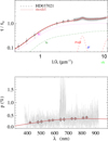 |
Fig. A.5 Notation same as in Fig. A.1 for HD 37021. |
| In the text | |
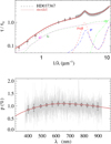 |
Fig. A.6 Notation same as in Fig. A.1 for HD 37367. |
| In the text | |
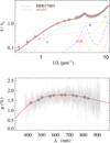 |
Fig. A.7 Notation same as in Fig. A.1 for HD 37903. |
| In the text | |
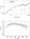 |
Fig. A.8 Notation same as in Fig. A.1 for HD 38087. |
| In the text | |
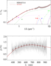 |
Fig. A.9 Notation same as in Fig. A.1 for HD 45314. |
| In the text | |
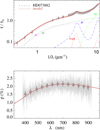 |
Fig. A.10 Notation same as in Fig. A.1 for HD 73882. |
| In the text | |
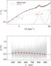 |
Fig. A.11 Notation same as in Fig. A.1 for HD 75309. |
| In the text | |
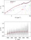 |
Fig. A.12 Notation same as in Fig. A.1 for HD 89137. |
| In the text | |
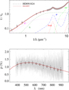 |
Fig. A.13 Notation same as in Fig. A.1 for HD 91824. |
| In the text | |
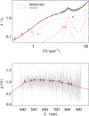 |
Fig. A.14 Notation same as in Fig. A.1 for HD 91983. |
| In the text | |
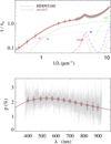 |
Fig. A.15 Notation same as in Fig. A.1 for HD 93160. |
| In the text | |
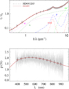 |
Fig. A.16 Notation same as in Fig. A.1 for HD 93205. |
| In the text | |
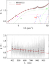 |
Fig. A.17 Notation same as in Fig. A.1 for HD 93222. |
| In the text | |
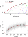 |
Fig. A.18 Notation same as in Fig. A.1 for HD 93632. |
| In the text | |
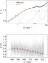 |
Fig. A.19 Notation same as in Fig. A.1 for HD 93843. |
| In the text | |
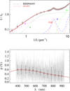 |
Fig. A.20 Notation same as in Fig. A.1 for HD 94493. |
| In the text | |
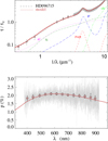 |
Fig. A.21 Notation same as in Fig. A.1 for HD 96715. |
| In the text | |
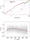 |
Fig. A.22 Notation same as in Fig. A.1 for HD 97484. |
| In the text | |
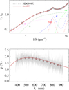 |
Fig. A.23 Notation same as in Fig. A.1 for HD 99953. |
| In the text | |
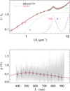 |
Fig. A.24 Notation same as in Fig. A.1 for HD 103779. |
| In the text | |
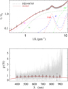 |
Fig. A.25 Notation same as in Fig. A.1 for HD 104705. |
| In the text | |
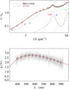 |
Fig. A.26 Notation same as in Fig. A.1 for HD 111934. |
| In the text | |
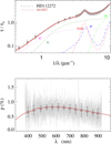 |
Fig. A.27 Notation same as in Fig. A.1 for HD 112272. |
| In the text | |
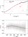 |
Fig. A.28 Notation same as in Fig. A.1 for HD 116852. |
| In the text | |
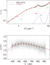 |
Fig. A.29 Notation same as in Fig. A.1 for HD 122879. |
| In the text | |
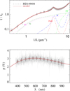 |
Fig. A.30 Notation same as in Fig. A.1 for HD 149404. |
| In the text | |
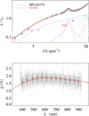 |
Fig. A.31 Notation same as in Fig. A.1 for HD 148379. |
| In the text | |
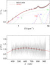 |
Fig. A.32 Notation same as in Fig. A.1 for HD 151804. |
| In the text | |
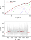 |
Fig. A.33 Notation same as in Fig. A.1 for HD 151805. |
| In the text | |
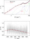 |
Fig. A.34 Notation same as in Fig. A.1 for HD 152235. |
| In the text | |
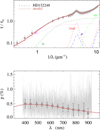 |
Fig. A.35 Notation same as in Fig. A.1 for HD 152248. |
| In the text | |
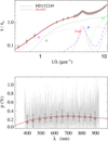 |
Fig. A.36 Notation same as in Fig. A.1 for HD 152249. |
| In the text | |
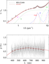 |
Fig. A.37 Notation same as in Fig. A.1 for HD 152408. |
| In the text | |
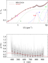 |
Fig. A.38 Notation same as in Fig. A.1 for HD 152424. |
| In the text | |
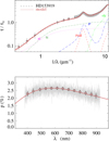 |
Fig. A.39 Notation same as in Fig. A.1 for HD 153919. |
| In the text | |
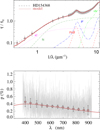 |
Fig. A.40 Notation same as in Fig. A.1 for HD 154368. |
| In the text | |
 |
Fig. A.41 Notation same as in Fig. A.1 for HD 163181. |
| In the text | |
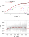 |
Fig. A.42 Notation same as in Fig. A.1 for HD 164073. |
| In the text | |
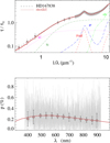 |
Fig. A.43 Notation same as in Fig. A.1 for HD 167838. |
| In the text | |
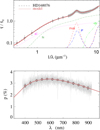 |
Fig. A.44 Notation same as in Fig. A.1 for HD 168076. |
| In the text | |
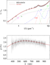 |
Fig. A.45 Notation same as in Fig. A.1 for HD 169454. |
| In the text | |
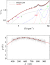 |
Fig. A.46 Notation same as in Fig. A.1 for HD 251204. |
| In the text | |
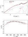 |
Fig. A.47 Notation same as in Fig. A.1 for HD 252325. |
| In the text | |
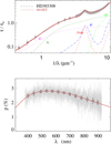 |
Fig. A.48 Notation same as in Fig. A.1 for HD 303308. |
| In the text | |
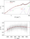 |
Fig. A.49 Notation same as in Fig. A.1 for HD 315023. |
| In the text | |
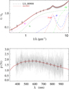 |
Fig. A.50 Notation same as in Fig. A.1 for LS–908. |
| In the text | |
Current usage metrics show cumulative count of Article Views (full-text article views including HTML views, PDF and ePub downloads, according to the available data) and Abstracts Views on Vision4Press platform.
Data correspond to usage on the plateform after 2015. The current usage metrics is available 48-96 hours after online publication and is updated daily on week days.
Initial download of the metrics may take a while.