Bulk Lorentz factors of gamma-ray bursts

G. Ghirlanda; F. Nappo; G. Ghisellini; A. Melandri; G. Marcarini; L. Nava; O. S. Salafia; S. Campana; R. Salvaterra

doi:10.1051/0004-6361/201731598

Home

All issues

Volume 609 (January 2018)

A&A, 609 (2018) A112

Full HTML

Free Access

Issue		A&A Volume 609, January 2018


Article Number		A112
Number of page(s)		19
Section		Extragalactic astronomy
DOI		https://doi.org/10.1051/0004-6361/201731598
Published online		25 January 2018

A&A 609, A112 (2018)

Bulk Lorentz factors of gamma-ray bursts

G. Ghirlanda¹^,2, F. Nappo³^,1, G. Ghisellini¹, A. Melandri¹, G. Marcarini², L. Nava¹^,5, O. S. Salafia²^,1, S. Campana¹ and R. Salvaterra⁴^,5

¹ INAF–Osservatorio Astronomico di Brera, via E. Bianchi 46, 23807 Merate, Italy
e-mail: giancarlo.ghirlanda@brera.inaf.it
² Dipartimento di Fisica G. Occhialini, Università di Milano Bicocca, Piazza della Scienza 3, 20126 Milano, Italy
³ Università degli Studi dell’Insubria, via Valleggio 11, 22100 Como, Italy
⁴ INAF–IASF Milano, via E. Bassini 15, 20133 Milano, Italy
⁵ INAF–Osservatorio Astronomico di Trieste, via G.B. Tiepolo, 11, 34143 Trieste, Italy

Received: 19 July 2017
Accepted: 11 October 2017

Abstract

Knowledge of the bulk Lorentz factor Γ₀ of gamma-ray bursts (GRBs) allows us to compute their comoving frame properties shedding light on their physics. Upon collisions with the circumburst matter, the fireball of a GRB starts to decelerate, producing a peak or a break (depending on the circumburst density profile) in the light curve of the afterglow. Considering all bursts with known redshift and with an early coverage of their emission, we find 67 GRBs (including one short event) with a peak in their optical or GeV light curves at a time t_p. For another 106 GRBs we set an upper limit t_p^UL. The measure of t_p provides the bulk Lorentz factor Γ₀ of the fireball before deceleration. We show that t_p is due to the dynamics of the fireball deceleration and not to the passage of a characteristic frequency of the synchrotron spectrum across the optical band. Considering the t_p of 66 long GRBs and the 85 most constraining upper limits, we estimate Γ₀ or a lower limit Γ₀^LL. Using censored data analysis methods, we reconstruct the most likely distribution of t_p. All t_p are larger than the time T_p,γ when the prompt γ-ray emission peaks, and are much larger than the time T_ph when the fireball becomes transparent, that is, t_p>T_p,γ>T_ph. The reconstructed distribution of Γ₀ has median value ~300 (150) for a uniform (wind) circumburst density profile. In the comoving frame, long GRBs have typical isotropic energy, luminosity, and peak energy ⟨ E_iso ⟩ = 3(8) × 10⁵⁰ erg, ⟨ L_iso ⟩ = 3(15) × 10⁴⁷ erg s^-1, and ⟨ E_peak ⟩ = 1(2) keV in the homogeneous (wind) case. We confirm that the significant correlations between Γ₀ and the rest frame isotropic energy (E_iso), luminosity (L_iso), and peak energy (E_p) are not due to selection effects. When combined, they lead to the observed E_p−E_iso and E_p−L_iso correlations. Finally, assuming a typical opening angle of 5 degrees, we derive the distribution of the jet baryon loading which is centered around a few 10^-6M_⊙.

Key words: gamma-ray burst: general / radiation mechanisms: non-thermal / relativistic processes

© ESO, 2018

1. Introduction

The relativistic nature of gamma-ray bursts (GRBs) was originally posed on theoretical grounds (Goodman 1986; Paczynski 1986; Krolik & Pier 1991; Fenimore et al. 1993; Baring & Harding 1997; Lithwick & Sari 2001): the small size of the emitting region, as implied by the observed millisecond variability, would make the source opaque due to γ–γ pair production unless it expands with bulk Lorentz factor Γ₀ ~ 100–1000 (e.g. Piran 1999). Refinements of this argument applied to specific GRBs (Abdo et al. 2009a,b; Ackermann et al. 2010a; Hascoët et al. 2012; Zhao et al. 2011; Zou & Piran 2010; Zou et al. 2011; Tang et al. 2015) led to some estimates of Γ₀. A direct confirmation that GRB outflows are relativistic was found in 970508 (Frail et al. 1997): the suppression of the observed radio variability ascribed to scintillation induced by Galactic dust provided an estimate of the source relativistic expansion. Similarly, the long-term monitoring in the radio band of GRB 030329 (Pihlström et al. 2007; Taylor et al. 2004, 2005) allowed to set limits on the expansion rate (Mesler et al. 2012).

In the standard fireball scenario, after an optically thick acceleration phase the ejecta coast with constant bulk Lorentz factor Γ₀ before decelerating due to the interaction with the external medium. Γ₀ represents the maximum value attained by the outflow during this dynamical evolution (see Kumar & Zhang for a recent review). Direct estimates of Γ₀ became possible in the last decade thanks to the early follow up of the afterglow emission. The detection of an early afterglow peak, t_p ~ 150–200 s, in the near-infrared light curve of GRB 060418 and GRB 060607A provided one of the first estimates of Γ₀ (Molinari et al. 2007).

The recent development of networks of robotic telescopes (ROTSE–III: Akerlof et al. 2003; GROCSE: Park et al. 1997; TAROT: Klotz et al. 2009; SkyNet: Graff et al. 2014; WIDGET: Urata et al. 2011; MASTER: Lipunov et al. 2004; Pi of the Sky: Burd et al. 2005; RAPTOR: Vestrand et al. 2002; REM: Zerbi et al. 2001; Watcher: Ferrero et al. 2010) has allowed us to follow up the early optical emission of GRBs. Systematic studies (Liang et al. 2010; Lü et al. 2012; Ghirlanda et al. 2012, G12 hereafter) derived the distribution of Γ₀ and its possible correlation with other observables. G12 found:

that different distributions of Γ₀ are obtained according to the density profile of the circumburst medium;

the existence of a correlation $Γ_{0}^{2} \propto L_{iso}$ $\hbox{$\Gamma_{0} ^2\propto L_{\rm iso}$}$ (tighter with respect to that with E_iso);

the presence of a linear correlation Γ₀ ∝ E_p.

As proposed by G12, the combination of these correlations provides a possible interpretation of the spectral energy correlations E_p−E_iso (Amati et al. 2002) and E_p−L_iso (Yonetoku et al. 2004) as the result of larger Γ₀ in bursts with larger luminosity/energy and peak energy. Possible interpretations of the correlations between Γ₀ and the GRB luminosity have been proposed in the context of neutrino or magneto–rotation powered jets (Lü et al. 2012; Lei et al. 2013). G12 (see also Ghirlanda et al. 2013a) showed that a possible relation between Γ₀ and the jet opening angle θ_jet could also justify the E_p−E_γ correlation (here E_γ is the collimation corrected energy).

In order to estimate Γ₀, we need to measure the onset time t_p of the afterglow. If the circumburst medium is homogeneous, this is revealed by an early peak in the light curve, corresponding to the passage from the coasting to the deceleration phase of the fireball. On the other hand, if a density gradient due to the progenitor wind is present, the bolometric light curve is constant until the onset time. However, also in the wind case, a peak could be observed if pair production ahead of the fireball is a relevant effect as discussed in G12, for example.

G12 considered 28 GRBs with a clear peak in their optical light curve, and included three GRBs with a peak in their GeV light curves (as observed by the Large Area Telescope – LAT – on board Fermi). Early t_p measurements are limited by the time needed to start the follow–up observations. The LAT (0.1–100 GeV), with its large field of view, performs observations simultaneously to the GRB prompt emission for GRBs happening within its field of view. The detection of an early peak in the GeV light curve, if interpreted as afterglow from the forward shock (e.g. Ghisellini et al. 2010; Kumar & Barniol Duran 2010), provides the estimate of the earliest t_p (i.e. corresponding to the largest Γ₀). In the short GRB 090510, the LAT light curve peaks at ~0.2 s corresponding to Γ₀ ~ 2000 (Ghirlanda et al. 2010; Ackermann et al. 2010b). Recently it has been shown that upper limits on Γ₀ can be derived from the non-detection of GRBs by the LAT (Nava et al. 2017) and that such limits are consistent with lower limits and detections reported in the literature.

Precise and fast localisations of GRB counterparts, routinely performed by Swift, coupled to efficient follow up by robotic telescope networks, allowed us to follow the optical emission starting relatively soon after the GRB trigger. However, a delay of a few hundred seconds can also induce a bias against the measure of early–intermediate t_p values (Hascoët et al. 2012). As argued by Hascoët et al. (2012), the distribution of Γ₀, derived through measured t_p, could lack intermediate to large values of Γ₀ (corresponding to intermediate to early values of t_p) and the Γ₀–E_iso correlation could be a boundary, missing several bursts with large Γ₀ (i.e. because of the lack of early t_p measurements).

For this reason, upper limits are essential to derive the distribution of Γ₀ in GRBs and its possible correlation with other prompt emission properties (E_iso, L_iso, and E_p) and, in general, to study the comoving frame properties of the population. To this aim, in this paper (i) we collect the available bursts with an optical t_p, expanding and revising the previously published samples; and (ii) we collect a sample of bursts with upper limits on t_p. Through this censored data sample we reconstruct the distribution of Γ₀ accounting (for the first time) for upper limits. We then employ Monte Carlo methods to study the correlations between Γ₀ and the rest frame isotropic energy/luminosity and peak energy.

The sample selection and its properties are presented in Sects. 2–4, respectively. The different formulae for the estimate of the bulk Lorentz factor Γ₀ appearing in the literature are presented and compared in Sect. 5. In Sect. 6 the distribution of Γ₀ and its correlation (Sect. 7) with E_iso, L_iso, and E_p are studied. Discussion and conclusions follow in Sect. 8. We assume a flat cosmology with h = Ω_Λ = 0.7.

2. The sample

We consider GRBs with measured redshift z and well constrained spectral parameters of the prompt emission. For these events it is possible to estimate the isotropic energy E_iso and luminosity L_iso and the rest frame peak spectral energy E_p (i.e. the peak of the νF_ν spectrum).

Γ₀ can be estimated from the measure of the peak t_p of the afterglow light curve interpreted as due to the deceleration of the fireball. We found in the literature 67 GRBs (66 long and 1 short) with an estimate of t_p (see Table A.1). Of these, 59 t_p are obtained from the optical and 8 from the GeV light curves. Through a systematic search of the literature we collected 106 long GRBs whose optical light curve, within one day of the trigger, decays with no apparent t_p. These GRBs provide upper limits $t_{p}^{UL}$ $\hbox{$t_{\rm p}^{\rm UL}$}$ . Details of the sample selection are reported in the following sections.

2.1. Afterglow onset t_p

G12 studied a sample of 30 long GRBs, with t_p measured from the optical (27 events) or from the GeV (3 events) light curves. We revise the sample of G12 with new data recently appearing in the literature, and we extend it, beyond GRB 110213A, including all new GRBs up to July 2016 with an optical or GeV afterglow light curve showing a peak t_p.

Bursts with a peak in their early X-ray emission are not included in our final sample because the X-ray can be dominated (a) by an emission component of “internal” origin, for example, due to the long lasting central engine activity (e.g. Ghisellini et al. 2007; Genet et al. 2007; Ioka et al. 2006; Panaitescu 2008; Toma et al. 2006; Nardini et al. 2010) and/or (b) by bright flares (Margutti et al. 2010)¹.

We excluded from our final sample (i) bursts with a multi–peaked optical light curve at early times²; and (ii) events with an optical peak preceded by a decaying light curve (e.g. GRB 100621A, GRB 080319C present in G12) since the early decay suggests the possible presence of a multi–peaked structure. The latter events, however, were included in the sample of $t_{p}^{UL}$ $\hbox{$t_{\rm p}^{\rm UL}$}$ (Sect. 2.2), considering the earliest epoch of their optical decay.

2.1.1. The gold sample

Table A.1 lists all the GRBs we collected. The “Gold” sample is composed of sources with a complete set of information, namely measured t_p (Col. 6) and spectral parameters (Cols. 3–5). It contains 49 events: 48 long GRBs plus the short event 090510. GRBs of the Gold sample have the label “(g)” at the end of their names reported in Col. 1 of Table A.1. The redshift z, rest frame peak energy E_p, isotropic energy and luminosity (E_iso and L_iso, respectively) are given in Table A.1. Eight out of 49 GRBs have their t_p measured from the GeV light curve as observed by the Fermi–LAT (labelled “L” or “SL” for the short GRB 090510).

For GRB 990123, GRB 080319B, and GRB 090102 reported in Table A.1, it has been proposed that the early optical emission (and the observed peak) is produced by either the reverse shock (RS; Bloom et al. 2009; Japelj et al. 2014; Sari & Piran 1999) or by a combination of forward and reverse shock (Gendre et al. 2010; Steele et al. 2009) or even by a two-component jet structure (e.g. Racusin et al. 2008,for GRB 080319B). We assume for these three GRBs that the peak is due to the outflow deceleration and include them in our sample.

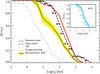Fig. 1

Cumulative distribution of the afterglow onset time t_p (red solid line) in the observer frame for the 66 long GRBs of the “Gold+Silver” sample. The black dashed line (marked with leftward arrows) is the cumulative distribution of 85 upper limits on t_p (filtered from Table A.1 according to $t_{p}^{UL} \leq 5 \times \max (t_{p}) ~ 11 500$ $\hbox{$t_{\rm p}^{\rm UL}\le 5\times \max(t_{\rm p})\sim11\,500$}$ s). The black solid line (shaded yellow region) is the reconstructed t_p distribution (95% confidence interval) accounting for $t_{p}^{UL}$ $\hbox{$t_{\rm p}^{\rm UL}$}$ through the Kaplan Meier estimator. The dotted and dot–dashed lines are the cumulative distributions of T₉₀ and T_p,γ (i.e. the time of the peak of the prompt emission light curve), respectively, for the 151 long GRBs. The distributions have been normalised to the respective sample size. Insert: Distribution of t_p (solid blue line) and of upper limits $t_{p}^{UL}$ $\hbox{$t_{\rm p}^{\rm UL}$}$ (dashed cyan line with leftward arrows) of the 50 GRBs of our sample (16 with t_p and 34 with $t_{p}^{UL}$ $\hbox{$t_{\rm p}^{\rm UL}$}$ ) also present in the Swift BAT complete sample (Salvaterra et al. 2012).

2.1.2. The silver sample

In our search we found 18 events with t_p but with poorly constrained prompt emission properties (E_p, E_iso, and L_iso). In most of these cases, the Swift Burst Alert Telescope (BAT) limited (15–150 keV) energy band coupled with a relatively low flux of the source prevent us from constraining the peak of the spectrum (E_p) even when it lies within the BAT energy range. Most of these BAT spectra were fitted by a simple power law model. Sakamoto et al. (2011) showed that, also in these cases, the E_p could be derived adopting an empirical correlation between the spectral index of the power law, fitted to the BAT spectrum, and E_p. This empirical correlation was derived and calibrated with those bursts where BAT can measure E_p. Alternatively, Butler et al. (2007, 2010) proposed a Bayesian method to recover the value of E_p for BAT spectra fitted by the simple power law model.

We adopted the values of E_p and E_iso calculated by Butler et al. (2007, 2010) for 15/18 GRBs in common with their list and the Sakamoto et al. (2011) relation for the remaining 3/18 events in order to exploit the measure of t_p also for these 18 bursts. Sakamoto et al. (2011) and Butler et al. (2007, 2010) study the time-integrated spectrum of GRBs. We estimated the luminosity L_iso = E_iso(P/F), where P and F are the peak flux and fluence, respectively, in the 15–150 keV energy range. GRBs of the “Silver” sample are labelled “(s)” in Table A.1.

While we made this distinction explicit for clarity, in what follows we use the total sample of t_p without any further distinction between the Gold and Silver samples.

2.2. Upper limits on t_p

The afterglow onset is expected within one day for typical GRB parameters (see Sect. 4). Several different observational factors, however, can prevent the measure of t_p. It is hard to construct a sample of upper limits $t_{p}^{UL}$ $\hbox{$t_{\rm p}^{\rm UL}$}$ . Hascoët et al. 2014 included some t_p in their analysis but without a systematic selection criterion.

In this paper we collect from the literature all the GRBs with known z and with an optical counterpart observed at least three times within one day of the trigger. If the light curve is decaying in time we set the upper limit $t_{p}^{UL}$ $\hbox{$t_{\rm p}^{\rm UL}$}$ corresponding to the earliest optical observation. Similar criteria apply if the long-lived afterglow emission is detected in the GeV energy range by the LAT. For several recent bursts, highly sampled early light curves are available. We excluded events with complex optical emission at early times and selected only those with an indication of a decaying optical flux.

The 106 GRBs with $t_{p}^{UL}$ $\hbox{$t_{\rm p}^{\rm UL}$}$ are reported in Table A.1. For the purposes of our analysis in the following we use a subsample of the 85 most constraining $t_{p}^{UL}$ $\hbox{$t_{\rm p}^{\rm UL}$}$ , that is, those with $t_{p}^{UL} \leq 11 500$ $\hbox{$t_{\rm p}^{\rm UL}\le 11\,500$}$ s which corresponds to five times the largest value of t_p of the Gold+Silver sample.

3. Sample properties

In this section we present the distribution of t_p (in the observer and rest frame) and study the possible correlation of the rest frame t_p with the observables of the prompt emission.

3.1. Distribution of the observer frame t_p

Figure 1 shows the cumulative distribution (red line) of the observer frame afterglow peak time t_p of long GRBs³. The distribution of upper limits $t_{p}^{UL}$ $\hbox{$t_{\rm p}^{\rm UL}$}$ is shown by the dashed black line (with leftward arrows). The distribution of measured t_p is consistent with that of the upper limits at the extremes, that is, below 30 s and above ~1000 s. In particular, the low–end of the distribution of t_p is mainly composed of bursts whose onset time is provided by the LAT data. Considering only GRBs with measured t_p (red line in Fig. 1), the (log) average t_p ~ 230 s while upper limits (dashed black line in Fig. 1) have a (log) average t_p ~ 160 s. The relative position of the two distributions (red and black dashed) suggests that if we considered only t_p measurements (as in G12; Liang et al. 2010; Lü et al. 2012) we would miss several intermediate–early onsets. This is confirmed also if we consider only the GRBs present in our sample which are part of the so called “BAT6” sample (Salvaterra et al. 2012). Indeed, this high flux cut sample of 58 Swift GRBs is 90% complete in redshift. There are 16 GRBs in our sample with measured t_p and 34 with $t_{p}^{UL}$ $\hbox{$t_{\rm p}^{\rm UL}$}$ in common with the BAT6 sample (i.e. 86% of the sample). Their t_p distribution (and the distribution of their $t_{p}^{UL}$ $\hbox{$t_{\rm p}^{\rm UL}$}$ ) is shown in the insert of Fig. 1. Similarly to the larger sample, the distribution of t_p for the BAT6 sample is close to that of upper limits $t_{p}^{UL}$ $\hbox{$t_{\rm p}^{\rm UL}$}$ .

In our sample nearly half of the bursts have t_p measured and half are upper limits. The distributions of t_p and $t_{p}^{UL}$ $\hbox{$t_{\rm p}^{\rm UL}$}$ overlap considerably ensuring that random censoring is present. Survival analysis (Feigelson & Nelson 1985) can be used to reconstruct the true distribution of t_p. We use the non–parametric Kaplan–Meier estimator (KM), as adapted by Feigelson & Nelson (1985) to deal with upper limits. The KM reconstructed CDF is shown by the solid black line in Fig. 1. The 95% confidence interval on this distribution (Miller 1981; Kalbfleish & Prentice 1980) is shown by the yellow shaded region in Fig. 1. The median value of the CDF is ⟨ t_p ⟩ = 60 ± 20 s (1σ uncertainty). We verified that, considering a more stringent subsample of upper limits, that is, $t_{p}^{UL} \leq 2 \times \max$ $\hbox{$t_{\rm p}^{\rm UL} \le 2\times \max$}$ (t_p), similar CDF and average values are obtained.

3.2. Distribution of the rest frame t_p

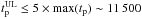
Figure 2 shows the cumulative distribution of t_p in the rest frame. Colour and symbols are the same as in Fig. 1. In particular we note that also in the rest frame the cumulative distribution of measured t_p (solid red line) is close to the distribution of upper limits (leftward arrows). The KM estimator leads to a reconstructed rest frame t_p distribution (solid black-yellow shaded curve) which is distributed between 1 and 10³ s with an average value of $2 0_{-5}^{+ 10}$ $\hbox{$20^{+10}_{-5}$}$ s. The insert of Fig. 2 shows the distribution of the onset time of the GRBs belonging to the complete Swift sample. Again the measured t_p distribution (solid blue line) is close to the distribution of upper limits, suggesting the presence of a selection bias against the measurement of the earliest t_p values which is, however, not due to the requirement of the measure of the redshift.

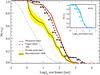Fig. 2

Cumulative distribution of the afterglow onset time t_p in the rest frame. Same symbols and colour code as in Fig. 1.

Table 1

Correlation between rest frame t_p/ (1 + z) and prompt emission properties (Fig. 4).

3.3. Comparison between t_p, T₉₀, and T_p,γ

One assumption for the estimate of Γ₀ from the measure of t_p (see Sect. 4) is that most of the kinetic energy of the ejecta has been transferred to the blast wave (so called “thin shell approximation” – Hascoët et al. 2014) which is decelerated by the circumburst medium. Therefore, we should expect that t_p be larger than the duration of the prompt emission, estimated by T₉₀. To check this hypothesis, we collected T₉₀ for the bursts of our sample: its distribution is shown by the grey dotted line in Fig. 1. A scatter plot showing T₉₀ vs. the observer frame t_p is shown in the top panel of Fig. 3: bursts with measured t_p are shown by the red filled circles (GRBs with t_p derived from the GeV–LAT light curve are shown by the star symbols), upper limits $t_{p}^{UL}$ $\hbox{$t_{\rm p}^{\rm UL}$}$ are also shown by the black (green for LAT bursts) symbols. The majority (80%) of GRBs lie below the equality line (dashed line in Fig. 3) having t_p>T₉₀. 20% of the bursts have t_p<T₉₀. A generalised Spearman’s rank correlation test (accounting also for upper limits – Isobe et al. (1986, 1990)) indicates no significant correlation between T₉₀ and t_p (at >3σ level of confidence).

The prompt emission of GRBs can be highly structured with multiple peaks separated by quiescent times. While T₉₀ is representative of the overall duration of the burst, another interesting timescale is the peak time of the prompt emission light curve T_p,γ. This time corresponds to the emission of a considerable fraction of energy during the prompt and it is worth comparing it with t_p. The distribution of T_p,γ is shown by the dot–dashed line in Fig. 1. The bottom panel of Fig. 3 compares T_p,γ with t_p. Noteworthily, no GRB has t_p<T_p,γ. There are only two upper limits $t_{p}^{UL}$ $\hbox{$t_{\rm p}^{\rm UL}$}$ from the early follow up of the GeV light curve (green arrows in the bottom panel of Fig. 3) which lie above the equality line. However, the large uncertainties in these two bursts (090328 and 091003) on their GeV light curve at early times (Panaitescu 2017) make them also compatible with having t_p>T_p,γ. Again, the Spearman’s generalised test results in no significant correlation between t_p and T_p,γ.

Fig. 3

Top panel: GRB duration T₉₀ vs. afterglow peak time t_p. GRBs with measured t_p are shown with red circles (green stars for LAT bursts). Upper limits on t_p are shown by the black arrows (green arrows for LAT GRBs). Bottom panel: time of the peak of the prompt emission light curve T_p,γ vs. t_p. Same symbols and colours as in the top panel. In both panels the equality is shown by the dashed line and the short GRB 090510 is shown by the green square.

3.4. Empirical correlations

We study the correlation between the onset time t_p in the rest frame and the energetic of GRBs. Figure 4 shows t_p/(1 + z) vs. the prompt emission isotropic energy E_iso, isotropic luminosity L_iso and rest frame peak energy E_p.

GRBs with measured t_p (red circles and green stars in Fig. 4) show significant correlations (chance probabilities <10^-5 – Table 1) shown by the red solid lines (obtained by a least square fit with the bisector method) in the panels of Fig. 4. The correlation parameters (slope and normalisation) obtained only with t_p are reported in the left part of Table 1.

Upper limits $t_{p}^{UL}$ $\hbox{$t_{\rm p}^{\rm UL}$}$ (black downward arrows in Fig. 4) are distributed in the same region of the planes occupied by t_p. Figure 4 shows also the lower limits on $t_{p}^{LL}$ $\hbox{$t_{\rm p}^{\rm LL}$}$ (grey upward arrows) derived assuming that t_p>T_p,γ.

The 85 GRBs without a measured t_p should have their onset $T_{p,γ} < t_{p} < t_{p}^{UL}$ $\hbox{$T_{\rm p,\gamma} < t_{\rm p} < t_{\rm p}^{\rm UL}$}$ corresponding to the vertical interval limited by the grey and black arrows in Fig. 4. Indeed, the reconstructed distribution of t_p (shown by the solid black line in Fig. 1) is bracketed by the cumulative distribution of T_p,γ on the left–hand side (dot–dashed grey line in Fig. 1) and by the distribution of $t_{p}^{UL}$ $\hbox{$t_{\rm p}^{\rm UL}$}$ on the right–hand side (dashed black line in Fig. 1).

In order to evaluate the correlations of Fig. 4 combining measured t_p and upper/lower limits we adopted a Monte Carlo approach. We assume that the KM estimator provides the distribution of t_p of the population of GRBs shown by the solid black line in Fig. 1. For each of the 85 GRBs with upper limits we extract randomly from the reconstructed t_p distribution a value of t_p (requiring that the extracted value t_p(i) falls within the range $T_{p,γ} (i) \leq t_{p} (i) \leq t_{p}^{UL} (i)$ $\hbox{$T_{\rm p,\gamma} (i)\le t_{\rm p} (i)\le t_{\rm p}^{\rm UL} (i)$}$ – where i runs from 1 to 85) and combine them with the 66 GRBs with measured t_p to compute the correlation (using the bisector method). We repeat this random extraction obtaining 10⁵ random samples and compute the average values of the Spearman’s rank correlation coefficient, of its chance probability, and of the slope and normalisation of the correlations (fitted to the 10⁵ randomly generated samples). In Fig. 4, the average correlation obtained through this Monte Carlo method is shown by the dot-dashed black line. The average values of the rank correlation coefficient, its probability, and the correlation parameters (slope and normalisation) are reported in the right section of Table 1.

These results show that significant correlations exist between the observables (i.e. fully empirical at this stage). A larger energy/luminosity/peak energy corresponds to an earlier t_p. The distribution of upper ( $t_{p}^{UL}$ $\hbox{$t_{\rm p}^{\rm UL}$}$ ) and lower (T_p,γ) limits in the planes of Fig. 4 show that these planes cannot be uniformly filled with points, further supporting the existence of these correlations.

Fig. 4

Left panel: t_p/ (1 + z) vs. E_iso. GRBs with estimates of t_p are shown with filled red circles (green symbols for LAT events). Upper limits on t_p (Table A.1) are shown by the black arrows (green arrows for LAT events). Middle panel: t_p/ (1 + z) vs. L_iso. Right panel: t_p/ (1 + z) vs. E_p. In all panels the short GRB 090510 is shown by the green square symbol.

4. On the origin of the afterglow peak time t_p

In the following we assume that the afterglow peak t_p is produced by the fireball deceleration. However, other effects can produce an early peak in the afterglow light curve: t_p can be due to the passage across the observation band of the characteristic frequencies of the synchrotron spectrum. In this case, however, any of the characteristic synchrotron frequencies should lie very close to the observation band at the time of the peak.

The synchrotron injection frequency is (Panaitescu & Kumar 2000): $ν_{inj} (t) = 0.92 \times 10^{13} ϵ_{B, - 2}^{1 / 2} ϵ_{e, - 1}^{2} (E_{iso, 53} / η)^{1 / 2} t^{- 3 / 2} (1 + z)^{-1} Hz,$ $\begin{equation} \nu_{\rm inj}(t)=0.92\times10^{13}\epsilon_{\rm B,-2}^{1/2}\epsilon_{\rm e,-1}^{2}(E_{\rm iso,53}/\eta)^{1/2}t^{-3/2}(1+z)^{-1} \,\,\,\,\, {\rm Hz} \label{nuinj} , \end{equation}$ (1)where ϵ_e and ϵ_B represent the fraction of energy shared between electrons and magnetic field at the shock and η is the efficiency of conversion of kinetic energy to radiation (i.e. E_iso,53/η represents the kinetic energy in units of 10⁵³ ergs in the blast wave). Here t is measured in days in the source rest frame. The above expression for ν_inj(t) is valid either if the circumburst medium has constant density or if its density decreases with the distance from the source as r^-2 (wind medium); in the latter case only the normalisation constant is larger by a factor ~2.

Fig. 5

Injection frequency at the t_p for each GRB. The optical-R frequency is show by the horizontal line. The injection frequency is shown for the homogeneous and wind case with red and blue symbols. GRBs with t_p from the LAT light curve are shown with star symbols. The scaling t^{− 3/2} of the injection frequency is shown for reference (it is not a fit) by the dashed line. Vertical bars, shown only for the red symbols, represent the position of the injection frequency obtained assuming ϵ_B in the range 10^-4−10^-1.

Figure 5 shows ν_inj(t = t_p) (red and blue symbols for the homogeneous or wind medium case and stars for the LAT bursts) with respect to the optical R frequency (solid horizontal line). We assumed typical values of the shock parameters: ϵ_B = 0.01 and ϵ_e = 0.1 and an efficiency η = 20% (Nava et al. 2014; Beniamini et al. 2015). The value ϵ_e = 0.1 is consistent with Beniamini & van der Horst (2017) and Nava et al. (2014) who recently found a narrow distribution of this parameter as inferred from the analysis of the radio and GeV afterglow, respectively. ϵ_B is less constrained and has a wider dispersion, between 10^-4 and 10^-1 (Granot & van der Horst 2014; Santana et al. 2014; Zhang et al. 2015; Beniamini et al. 2016), which translates into a factor of 10 for the value of ν_inj (vertical lines in Fig. 5) obtained assuming ϵ_B = 0.01 (open circles in Fig. 5) . In order to account for this uncertainty we show, as vertical lines in Fig. 5 (for the open circles only for clarity), the possible range of frequencies that are obtained assuming ϵ_B ∈ [10^-4,10^-1]. In all bursts, the injection frequency, when the afterglow peaks (i.e. at t_p), is above the optical band and it cannot produce the peak as we see it⁴.

However, one may argue that the above argument depends on the assumed typical values of ϵ_e and ϵ_B. Consider, for example, the homogeneous case s = 0. In order to “force” ν_inj = ν_opt,R = 4.86 × 10¹⁴ Hz at t = t_p and reproduce the observed flux at the peak F_p, one would require a density of the ISM: $n_{0} (s = 0) = 1.3 \times 10^{3} D_{28}^{4} E_{53}^{-1} ϵ_{e, - 1}^{4} t_{p, \sec, - 2}^{-3} (1 + z)^{- 4 / 3} F_{p, mJy}^{2} c m^{-3},$ $\begin{equation} n_{0}(s=0)=1.3\times10^{3}\,\, D_{28}^{4} E_{53}^{-1} \epsilon_{\rm e,-1}^{4} t_{\rm p,sec,-2}^{-3}(1+z)^{-4/3} F_{\rm p,mJy}^2\,\,\, {\rm cm^{-3}} , \end{equation}$ (2)where D₂₈ is the luminosity distance in units of 10²⁸ cm and t_p,sec,−2 is the rest frame peak time, now expressed in units of 100 s. For typical peak flux of 10 mJy we should have densities ~ 10⁵ cm^-3.

The other synchrotron characteristic frequency which could evolve and produce a peak when passing across the optical band is the cooling frequency ν_cool. For the homogeneous medium $ν_{cool} = 3.7 \times 10^{14} ϵ_{B, - 2}^{- 3 / 2} (E_{iso, 53} / η)^{- 1 / 2} n^{-1} t_{p}^{- 1 / 2} (1 + z)^{-1} (Y + 1)^{-2}$ $\hbox{$\nu_{\rm cool}=3.7\times10^{14}\epsilon_{\rm B,-2}^{-3/2}(E_{\rm iso,53}/\eta)^{-1/2}n^{-1}t_{\rm p}^{-1/2}(1+z)^{-1}(Y+1)^{-2}$}$ Hz, where n is the number density of the circum burst medium and Y the Compton parameter (Panaitescu & Kumar 2000). In this case, the portion of the synchrotron spectrum which could produce a peak is ν < ν_cool, under the assumption that ν_cool <ν_inj, and the flux evolution should be F(t) ∝ t^1/6 (Panaitescu 2017; Sari et al. 1998). This is much shallower than the rising slopes of the afterglow emission of most of the bursts before t_p (Liang et al. 2013). In the wind case, the cooling break increases with time ∝t^1/2 and, if transitioning accross the observing band from below, it should produce a decaying afterglow flux F(t) ∝ t^{− 1/4} and not a peak.

Therefore, we are confident that t_p cannot be produced by any of the synchrotron frequencies crossing the optical band and it can be interpreted as due to the deceleration of the fireball and used to estimate Γ₀.

5. Estimate of Γ₀

In this section we revise, in chronological order, the different methods and formulae proposed for estimating the bulk Lorentz factor Γ₀ (Ghirlanda et al. 2012; Ghisellini et al. 2010; Molinari et al. 2007; Nava et al. 2017; Sari & Piran 1999). The scope is to compare these methods and quantify their differences. We consider only the case of an adiabatic evolution of the fireball propagating in an external medium with a power law density profile n(R) = n₀R^{− s}. The general case of a fully radiative (and intermediate) emission regime is discussed in Nava et al. (2013). In Sect. 5 we present the results, that is, estimates of Γ₀, for the two popular cases s = 0 (homogeneous medium) and s = 2 (wind medium). The estimate and comparison of Γ₀ in these two scenarios for a sample of 30 GRBs was presented, for the first time, in G12.

During the coasting phase the bulk Lorentz factor is constant (Γ = Γ₀) and the bolometric light curve of the afterglow scales as L_iso ∝ t^2−s. After the deceleration time, Γ₀ starts to decrease and, in the adiabatic case, the light curve scales as L_iso ∝ t^-1 independently from the value of s.

Therefore, for a homogeneous medium (s = 0) the light curve has a peak, while in the wind case (s = 2) the light curve should be flat before t_p and steeper afterwards⁵. Γ₀ is the bulk Lorentz factor corresponding to the coasting phase. It is expected that the outflow is discontinuous with a distribution of bulk Lorentz factors (e.g. to develop internal shocks). Γ₀ represents the average bulk Lorentz factor of the outflow during the coasting phase.

5.1. Sari & Piran (1999)

In (Sari & Piran 1999, hereafter SP99) Γ₀ is derived assuming that t_p corresponds to the fireball reaching the deceleration radius R_dec. This is defined as the distance from the central engine, where the mass of the interstellar medium m(R_dec), swept up by the fireball, equals M₀/ Γ₀: $m (R_{dec}) = \frac{M_{0}}{Γ_{0}} = \frac{E_{0}}{Γ_{0}^{2} c^{2}},$ $\begin{equation} m(R_{\rm dec}) \, =\, {M_0\over \Gamma_0}\, =\, {E_0\over \Gamma_0^2 c^2 } , \end{equation}$ (3)where E₀ is the isotropic equivalent kinetic energy of the fireball after the prompt phase.

SP99 assume $t_{dec} = R_{dec} / (2 c Γ_{0}^{2})$ $\hbox{$t_{\rm dec} = R_{\rm dec}/(2c\Gamma_0^2)$}$ as the link between the deceleration time t_dec and R_dec. This assumption corresponds implicitly to considering that the fireball travels up to R_dec with a constant bulk Lorentz factor equal to Γ₀, or, in other words, that the deceleration starts instantaneously at this radius. Instead, the deceleration of the fireball starts before R_dec. This approximation underestimates the deceleration time t_dec and, consequently, underestimates Γ₀: $Γ_{0}^{(SP 99)} = {[(\frac{3 - s}{2^{5 - s} π}) (\frac{E_{0}}{n_{0} m_{p} c^{5 - s}})]}^{\frac{1}{8 - 2 s}} t_{p, z}^{- \frac{3 - s}{8 - 2 s}},$ $\begin{equation} \Gamma_{0}^{\rm (SP99)} = \left[\left(\frac{3-s}{2^{5-s}\pi}\right) \left(\frac{E_0}{n_0 m_{\rm p}c^{5-s}}\right)\right]^{\frac{1}{8-2s}} t_{\rm p, \it z}^{-\frac{3-s}{8-2s}}, \label{eq:SP99} \end{equation}$ (4)where t_p,z ≡ t_p/ (1 + z). The original formula reported in SP99 is valid only for a homogeneous medium. Here, Eq. (2) has been generalised for a generic power law density profile medium.

5.2. Molinari et al. (2007)

Molinari et al. (2007, hereafter M07) introduce a new formula for Γ₀, obtained from SP99 by modifying the assumption on R_dec. They, realistically, consider that the deceleration begins before R_dec so that Γ_dec< Γ₀. Under this assumption, $m (R_{dec}) = M_{0} / Γ_{dec} = E_{0} / (Γ_{dec}^{2} c^{2})$ $\hbox{$m(R_{\rm dec})=M_0/\Gamma_{\rm dec}=E_0/(\Gamma_{\rm dec}^2 c^2)$}$ and $t_{dec} = R_{dec} / (2 c Γ_{dec}^{2})$ $\hbox{$t_{\rm dec} = R_{\rm dec}/(2c\Gamma_{\rm dec}^2)$}$ . However, they assume Γ_dec = Γ₀/ 2 obtaining: $Γ_{0}^{(M 07)} = 2 {[(\frac{3 - s}{2^{5 - s} π}) (\frac{E_{0}}{n_{0} m_{p} c^{5 - s}})]}^{\frac{1}{8 - 2 s}} t_{p, z}^{- \frac{3 - s}{8 - 2 s}} .$ $\begin{equation} \label{eq:M07} \Gamma_{0}^{\rm (M07)} = 2\left[\left(\frac{3-s}{2^{5-s}\pi}\right) \left(\frac{E_0}{n_0 m_{\rm p}c^{5-s}}\right)\right]^{\frac{1}{8-2s}} t_{\rm p, \it z}^{-\frac{3-s}{8-2s}} . \end{equation}$ (5)This estimate of Γ₀ is a factor 2 larger than that obtained by SP99: as discussed in Nava et al. (2013), M07 overestimate⁶ the deceleration radius by a factor ~ 2 and, consequently, the value of Γ₀ is overestimated by the same factor. This is consistent with the results of numerical one-dimensional (1D) simulations of the blast wave deceleration (Fukushima et al. 2017). Their results suggest that Γ₀ should be a factor ~2.8 smaller than that derived (e.g. by Liang et al. 2010) through Eq. (5).

5.3. Ghisellini et al. (2010)

A new method to calculate the afterglow peak time t_p is presented in (Ghisellini et al. 2010, hereafter G10). This method does not rely on the definition of the deceleration radius as in SP99 and M07. G10 derive t_p by equating the two different analytic expressions for the bolometric luminosity as a function of the time L(t) during the coasting phase and during the deceleration phase⁷.

The relation linking the radius and the time is assumed to be: R = 2actΓ², where a = 1 during the coasting phase and a> 1 during the deceleration one. In the latter case, its value depends on the relation between the bulk Lorentz factor Γ and the radius R: for an adiabatic fireball, for instance, integration of dR = 2cΓ²dt, assuming Γ ∝ R^{− (3−s)/2} according to the self–similar solution of Blandford & McKee (1976, hereafter BM76), we obtain a = 4−s.

G10 assume a relation between Γ and R which is formally identical to the BM76 solution but with a different normalisation factor: $Γ (R) = \sqrt{\frac{E_{0}}{m (R) c^{2}}} = \sqrt{\frac{(3 - s) E_{0}}{4 π n_{0} m_{p} c^{2} R^{3 - s}}},$ $\begin{equation} \label{eq:gR} \Gamma(R)=\sqrt{\frac{E_0}{m(R)c^2}}=\sqrt{\frac{(3-s)E_0}{4\pi n_0 m_{\rm p} c^{2} R^{3-s}}} , \end{equation}$ (6)where m(R) is the interstellar mass swept by the fireball up to the radius R.

In G10, the authors are interested in the determination of the peak time of the light curve, but that expression can also be used to determine the initial Lorentz factor Γ₀. The expression, generalised for a power law profile of the external medium density, is: $\begin{matrix} Γ_{0}^{(G 10)} = {[(\frac{3 - s}{2^{5 - s} π (4 - s)^{3 - s}}) (\frac{E_{0}}{n_{0} m_{p} c^{5 - s}})]}^{\frac{1}{8 - 2 s}} t_{p, z}^{- \frac{3 - s}{8 - 2 s}} . \end{matrix}$ $\begin{eqnarray} \label{eq:G10} \Gamma_{0}^{\rm (G10)} = \left[\left(\frac{3-s}{2^{5-s}\pi(4-s)^{3-s}}\right) \left(\frac{E_0}{n_0 m_{\rm p}c^{5-s}}\right)\right]^{\frac{1}{8-2s}} t_{\rm p, \it z}^{-\frac{3-s}{8-2s}} . \end{eqnarray}$ (7)This estimate of Γ₀ is even lower than that of SP99 and, therefore, we can reasonably presume that also this value of Γ₀ will be underestimated with respect to the real one⁸.

5.4. Ghirlanda et al. (2012)

Ghirlanda et al. (2012) derive another formula to estimate Γ₀, based on the method proposed in G10, that is, intersecting the asymptotic behaviours of the bolometric light curve during the coasting phase with that during the deceleration phase. In order to describe Γ(R) in the deceleration regime, G12 use the BM76 solution with the correct (with respect to G10) normalisation factor: $Γ (R) = \sqrt{\frac{(17 - 4 s) E_{0}}{(12 - 4 s) m (R) c^{2}}} = \sqrt{\frac{(17 - 4 s) E_{0}}{16 π n_{0} m_{p} c^{2} R^{3 - s}}} \cdot$ $\begin{equation} \label{eq:BM76} \Gamma(R)=\sqrt{\frac{(17-4s)E_0}{(12-4s)m(R)c^2}}=\sqrt{\frac{(17-4s)E_0}{16\pi n_0 m_{\rm p} c^2 R^{3-s}}}\cdot \end{equation}$ (8)The relation between radius and time is that presented in G10: 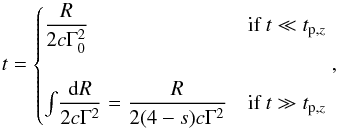$t = {\begin{matrix} if t ≪ t_{p, z} \\ if t ≫ t_{p,z} \end{matrix},$ $\begin{equation} t = \begin{cases} \dfrac{R}{2c \Gamma_0^2} & \mbox{if } t \ll t_{\rm p, \it z} \\ \\ {\LARGE\int}\dfrac{{\rm d}R}{2c\Gamma^2}= \dfrac{R}{2(4-s)c\Gamma^2} & \mbox{if } t \gg t_{\rm p,\it z} \end{cases} , \end{equation}$ (9)where t ≪ t_p,z (t ≫ t_p,z) corresponds to the coasting (deceleration) phase. The authors use these relations to obtain analytically the bolometric light curves before and after the peak and extrapolate them to get the intersection time which is used to infer Γ₀: $\begin{matrix} Γ_{0}^{(G 12)} = {[(\frac{17 - 4 s}{2^{8 - s} π (4 - s)}) (\frac{E_{0}}{n_{0} m_{p} c^{5 - s}})]}^{\frac{1}{8 - 2 s}} t_{p, z}^{- \frac{3 - s}{8 - 2 s}} . \end{matrix}$ $\begin{eqnarray} \label{eq:G12} \Gamma_{0}^{\rm (G12)} = \left[\left(\frac{17-4s}{2^{8-s}\pi(4-s)}\right) \left(\frac{E_0}{n_0 m_{\rm p}c^{5-s}}\right)\right]^{\frac{1}{8-2s}} t_{\rm p, \it z}^{-\frac{3-s}{8-2s}} . \end{eqnarray}$ (10)The main difference with respect to the formula of G10 comes from the normalisation factor of the BM76 solution and corresponds to a factor [(17−4s)/(12−4s)] ^1/2.

5.5. Nava et al. (2013)

Nava et al. (2013, hereafter N13) propose a new model to describe the dynamic evolution of the fireball during the afterglow emission. With this model, valid for an adiabatic or full and semi–radiative regime, N13 compute the bolometric afterglow light curves and derive a new analytic formula for Γ₀. They rely on the same method (intersection of coasting/deceleration phase luminosity solution) already used by G10 and G12, but with a more realistic description of the dynamics of the fireball, provide an analytic formula for the estimate of Γ₀ in the case of a purely adiabatic evolution (Eq. (11)), and a set of numerical coefficients to be used for the full or semi–radiative evolution.

In the rest of the present work we will adopt the formula of N13 to compute Γ₀ so we report here their equation: $Γ_{0}^{(N 13)} = {[\frac{(17 - 4 s) (9 - 2 s) 3^{2 - s}}{2^{10 - 2 s} π (4 - s)} (\frac{E_{0}}{n_{0} m_{p} c^{5 - s}})]}^{\frac{1}{8 - 2 s}} t_{p, z}^{- \frac{3 - s}{8 - 2 s}} .$ $\begin{equation} \label{eq:N13} \Gamma_{0}^{\rm (N13)} = \left[\frac{(17-4s)(9-2s)3^{2-s}}{2^{10-2s}\pi(4-s)} \left(\frac{E_0}{n_0 m_{\rm p}c^{5-s}}\right)\right]^{\frac{1}{8-2s}} t_{\rm p, \it z}^{-\frac{3-s}{8-2s}} . \end{equation}$ (11)The difference with respect to the formula of G12 is due to the different relation between the shock radius R and the observed time t. All the preceding derivations assume that most of the observed emission comes from the single point of the expanding fireball that is moving exactly toward the observer, along the line of sight. Actually, the emitted radiation that arrives at time t to the observer does not come from a single point, but rather from a complex surface (Equal Arrival Time Surface, EATS) that does not coincide with the surface of the shock front. N13 avoid the rather complex computation of the EATSs, adopting a relation t(R) proposed by Waxman (1997) to relate radii to times. For simplicity, in the ultra–relativistic approximation: 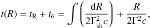$t (R) = t_{R} + t_{θ} = \int (\frac{d R}{2 Γ_{sh}^{2} c}) + \frac{R}{2 Γ^{2} c},$ $\begin{equation} \label{eq:timeWAX} t(R) = t_{\rm R} + t_{\rm \theta} = \int\left(\frac{{\rm d}R}{2\Gamma_{\rm sh}^2c}\right)\,+\frac{R}{2\Gamma^2c}, \end{equation}$ (12)where Γ_sh = 2Γ is the shock Lorentz factor. The time is the sum of a radial time t_R, that is the delay of the shock front with respect to the light travel time at radius R and an angular time t_θ, that is the delay of photons emitted at the same radius R but at larger angles with respect to the line of sight. Using the correct dynamics, N13 obtain the relation between observed time and shock front radius: 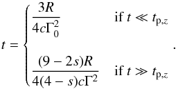$t = {\begin{matrix} if t ≪ t_{p, z} \\ if t ≫ t_{p,z} \end{matrix} .$ $\begin{equation} t = \begin{cases} \dfrac{3R}{4c \Gamma_0^2} & \mbox{if } t \ll t_{\rm p, \it z} \\ \\ \dfrac{(9-2s)R}{4(4-s)c\Gamma^2} & \mbox{if } t \gg t_{\rm p, \it z} \end{cases} . \end{equation}$ (13)N13 use these relations to obtain analytically the bolometric light curve during the coasting and the deceleration phase and, from their intersection time, estimate Γ₀ through Eq. (11).

Table 2

Comparison between the different methods of estimating Γ₀ found in literature.

5.6. Nappo et al. (2014)

Nappo et al. (2014, hereafter N14) do not introduce directly a new formula to estimate Γ₀, but show a new way (valid only in the ultra–relativistic regime Γ ≫ 1) to convert the shock radius R into the observer time t, bypassing the problem of the calculation of the EATSs. They assume that most of the observed emission is produced in a ring with aperture angle sinθ = 1/Γ around the line of sight. The differential form of the relation between observed time and radius can be written as dR = cΓ²dt, that differs from the analogous relations of G10 and G12 by a factor 2.

Using this simplified relation coupled to the dynamics of N13 we derive a new expression for Γ₀: $Γ_{0}^{(N 14)} = {[(\frac{(17 - 4 s)}{16 π (4 - s)}) (\frac{E_{0}}{n_{0} m_{p} c^{5 - s}})]}^{\frac{1}{8 - 2 s}} t_{p, z}^{- \frac{3 - s}{8 - 2 s}} .$ $\begin{equation} \label{eq:N14} \Gamma_{0}^{\rm (N14)} = \left[\left(\frac{(17-4s)}{16\pi(4-s)}\right) \left(\frac{E_0}{n_0 m_{\rm p}c^{5-s}}\right)\right]^{\frac{1}{8-2s}} t_{\rm p, \it z}^{-\frac{3-s}{8-2s}} . \end{equation}$ (14)We show in the following paragraph that this expression provides results that are very similar to those obtained with the formula of N13, proving that the approximation on the observed times is compatible with that suggested by N13 and before by Waxman (1997).

5.7. Comparison between different methods

All the previous expressions have the same dependencies on the values of E₀, n₀, and t_p,z. They differ only by a numeric factor and can be summarised in one single expression: 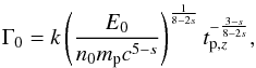$Γ_{0} = k {(\frac{E_{0}}{n_{0} m_{p} c^{5 - s}})}^{\frac{1}{8 - 2 s}} t_{p, z}^{- \frac{3 - s}{8 - 2 s}},$ $\begin{equation} \label{eq:total} \Gamma_{0} = k \left(\frac{E_0}{n_0 m_{\rm p}c^{5-s}}\right)^{\frac{1}{8-2s}} t_{\rm p, \it z}^{-\frac{3-s}{8-2s}} , \end{equation}$ (15)where k is a numeric factor that depends on the chosen method and on the power law index of the external medium density profile. In Table 2 we list the different values of k for the various models and we show the comparison between the different estimates of Γ₀ for both a homogeneous and a wind medium. All the possible estimates of Γ₀ are within a factor ~ 2 of the estimate of N13; in particular the value provided by the N14 formula (Eq. (14)) is similar to N13 within a few percent.

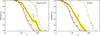Fig. 6

Cumulative distribution of Γ₀ for GRBs with measured t_p (red solid line). The distribution of lower limits $Γ_{0}^{LL}$ $\hbox{$\Gamma_{0}^{\rm LL}$}$ , derived for GRBs with an upper limit on the onset time $t_{p}^{UL}$ $\hbox{$t_{\rm p}^{\rm UL}$}$ , is shown by the dashed black curve (with rightward arrows). Assuming t_p ≥ T_p,γ the distribution of upper limits on Γ₀ is shown by the dotted grey line (with leftward arrows). The most stringent limit on the distribution of Γ₀ is shown by the green solid line which assumes that deceleration radius R_dec ≥ R(τ = 1), that is, the transparency radius (Eq. (16)). Joining estimates of Γ₀ and lower limits $Γ_{0}^{LL}$ $\hbox{$\Gamma_{0}^{\rm LL}$}$ the reconstructed (through the KM estimator) distribution of Γ₀ is shown by the solid black line (and its 95% uncertainty by the yellow shaded region). The distributions are normalised to their respective number of elements. The two panels (right and left, respectively) show the case of a homogeneous (s = 0) and wind (s = 2) medium.

6. Results

Through Eq. (11) we estimate:

the bulk Lorentz factors Γ₀ of the 67 GRBs with measured t_p;

lower limits $Γ_{0}^{LL}$ $\hbox{$\Gamma_{0}^{\rm LL}$}$ for the 85 bursts with upper limits on the onset time $t_{p}^{UL}$ $\hbox{$t_{\rm p}^{\rm UL}$}$ ;

upper limit $Γ_{0}^{UL}$ $\hbox{$\Gamma_{0}^{\rm UL}$}$ for the 85 bursts with lower limits on the onset time $t_{p}^{LL} = T_{p,γ}$ $\hbox{$t_{\rm p}^{\rm LL}=T_{\rm p,\gamma}$}$ .

We consider both a homogeneous density ISM (s = 0) and a wind density profile (s = 2). For the first case, we assume n₀ = 1 cm^-3. For the second case, n(r) = n₀r^-2 = Ṁ/ 4πr²m_pv_w where Ṁ is the mass-loss rate and v_w the wind velocity. For typical values (e.g. Chevalier & Li 1999) Ṁ = 10^-5M_⊙ yr^-1 and v_w = 10³ km s^-1, the normalisation of the wind case is $n_{0} = 10^{35} Ṁ {}_{-5}v_{w, - 3}^{-1}$ $\hbox{$n_{0}=10^{35} \dot{M}_{-5} v^{-1}_{w,-3}$}$ cm^-1.

In both cases we assume that the radiative efficiency of the prompt phase is η = 20% and estimate the kinetic energy of the blast wave in Eq. (11) as E₀ = E_iso/η. The assumed typical value for η is similar to that reported in Nava et al. (2014) and Beniamini et al. (2015) who also find a small scatter of this parameter. We notice that assuming different values of n₀ and η within a factor of 10 and 3 with respect to those adopted in our analysis would introduce a systematic difference in the estimate of Γ₀ corresponding to a factor ~1.5 (2.3) for s = 0(s = 2).

6.1. Distribution of Γ₀

Figure 6 shows the cumulative distribution of Γ₀. The solid red line is the distribution of Γ₀ for the 66 GRBs with a measure of t_p. The cumulative distribution of $Γ_{0}^{LL}$ $\hbox{$\Gamma_{0}^{\rm LL}$}$ is shown by the black dashed line (with rightward arrows) in Fig. 6. The cumulative distribution of $Γ_{0}^{UL}$ $\hbox{$\Gamma_{0}^{\rm UL}$}$ is shown by the dotted grey line (with leftward arrows) in Fig. 6. We note that while $Γ_{0}^{LL}$ $\hbox{$\Gamma_{0}^{\rm LL}$}$ is derived from the optical light curves decaying without any sign of the onset (i.e. providing $t_{p}^{UL}$ $\hbox{$t_{\rm p}^{\rm UL}$}$ ), the limit $Γ_{0}^{UL}$ $\hbox{$\Gamma_{0}^{\rm UL}$}$ is derived assuming that the onset time happens after the peak of the prompt emission (i.e. T_p,γ).

A theoretical upper limit on Γ₀ can be derived from the the transparency radius, that is, R(τ = 1) (Daigne & Mochkovitch 2002). The maximum bulk Lorentz factor attainable, if the acceleration is due to the internal pressure of the fireball (i.e. R ∝ Γ) is: 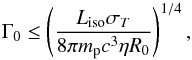$Γ_{0} \leq {(\frac{L_{iso} σ_{T}}{8 π m_{p} c^{3} η R_{0}})}^{1 / 4},$ $\begin{equation} \Gamma_{0}\le \left(\frac{L_{\rm iso}\sigma_{T}}{8\pi m_{\rm p} c^3 \eta R_{0}}\right)^{1/4} \label{eqtrans} , \end{equation}$ (16)where σ_T is the Thomson cross section and R₀ is the radius where the fireball is launched. We assume R₀ ~ 10⁸ cm. This is consistent with the value obtained from the modelling of the photospheric emission in a few GRBs Ghirlanda et al. (2013b). The cumulative distribution of upper limits on Γ₀ obtained through Eq. (16), substituting for each GRB its L_iso, is shown by the green solid line in Fig. 6 (with the leftward green arrows). This distribution represents the most conservative limit on Γ₀⁹.

Table 3

Average values and 68% confidence intervals on Γ₀ (derived with only measured t_p – red line in Fig. 6) or including lower limits $Γ_{0}^{LL}$ $\hbox{$\Gamma_{0}^{\rm LL}$}$ (derived from upper limits $t_{p}^{UL}$ $\hbox{$t_{\rm p}^{\rm UL}$}$ – black line in Fig. 6).

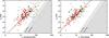Fig. 7

Correlation between the isotropic equivalent luminosity L_iso and the bulk Lorentz factor Γ₀. Estimates of Γ₀ from the measured afterglow onset t_p for 68 long GRBs (red filled circles and green filled stars) and the short GRB 090510 (green filled square symbol). Lower limits $Γ_{0}^{LL}$ $\hbox{$\Gamma_{0}^{\rm LL}$}$ (derived from upper limits on the onset time $t_{p}^{UL}$ $\hbox{$t_{\rm p}^{\rm UL}$}$ ) are shown by the rightward black arrows. Upper limits $Γ_{0}^{UL}$ $\hbox{$\Gamma_{0}^{\rm UL}$}$ (derived assuming that the afterglow onset time is larger than the peak time of the prompt emission, that is, t_p ≥ T_p,γ) are shown by the grey (leftward) arrows. Upper limit on Γ₀ imposed by the requirement that the deceleration radius is larger than the transparency radius is shown by the grey shaded triangular region (for two values of the radius R₀ where the fireball is formed – see Eq. (16)). The solid red line shows the correlation obtained with Γ₀ solely (bisector method), while the black dot–dashed line is the correlation obtained through the Monte Carlo method which accounts for the reconstructed distribution of Γ₀. Left and right panels show the case of a homogeneous and wind medium, respectively.

Similarly to the cumulative distributions of t_p, shown in Fig. 1, also the distributions of Γ₀ (red solid line) and the distribution of lower limits $Γ_{0}^{LL}$ $\hbox{$\Gamma_{0}^{\rm LL}$}$ (black dashed line) are very close to each other. While at low and high values of Γ₀ the two curves are consistent with one another, for intermediate values of Γ₀ the distribution of lower limits is very close to that of measured Γ₀. In the wind case (right panel of Fig. 6), the lower limits distribution violates the distribution of measured Γ₀. This suggests that the distribution of Γ₀ obtained only with measured t_p suffers from the observational bias related to the lack of GRBs with very early optical observations.

We used the KM estimator to reconstruct the distribution of Γ₀, combining measurements and lower limits, similarly to what has been done in Sect. 3.1 for t_p. The solid black line (with its 95% uncertainty) in Fig. 6 shows the most likely distribution of Γ₀ for the population of long GRBs under the assumption of a homogeneous ISM (left panel) and for a wind medium (right panel).

The median values of Γ₀ (reported in Table 3) are 320 and 150 for the homogeneous and wind case, respectively, and they are consistent within their 1σ confidence intervals. G12 found smaller average values of Γ₀ (i.e. 138 and 66 in the homogeneous and wind case, respectively) because of the smaller sample size (30 GRBs) and the non-inclusion of limits on Γ₀. Indeed, while the intermediate/small values of Γ₀ are reasonably well sampled by the measurements of t_p, the bias against the measure of large Γ₀ is due to the lack of small t_p measurements (the smallest t_p are actually provided by the still few LAT detections).

The reconstructed distribution of Γ₀ (black line in Fig. 6) is consistent with the distribution of upper limits derived assuming t_p ≥ T_p,γ (dotted grey distribution) in the homogeneous case. For the wind medium there could be a fraction of GRBs (~20%) whose t_p is smaller than the peak of the prompt emission. However, Fig. 6 shows that, both in the homogeneous and wind case, the reconstructed Γ₀ distribution is consistent with the limiting distribution (green line) derived assuming that the deceleration occurs after transparency is reached.

7. Correlations

G12 found correlations between the bulk Lorentz factor Γ₀ and the prompt emission properties of GRBs: $L_{iso} \propto Γ_{0}^{2}$ $\hbox{$L_{\rm iso} \propto \Gamma_{0}^{2}$}$ , $E_{iso} \propto Γ_{0}^{2}$ $\hbox{$E_{\rm iso} \propto\Gamma_{0}^{2}$}$ , and with a larger scatter, E_p ∝ Γ₀. Interestingly, combining these correlations leads to $E_{p} \propto E_{iso}^{0.5}$ $\hbox{$E_{\rm p} \propto E_{\rm iso} ^{0.5}$}$ and $E_{p} \propto L_{iso}^{0.5}$ $\hbox{$E_{\rm p} \propto L_{\rm iso} ^{0.5}$}$ which are the E_p−E_iso (Amati et al. 2002) and Yonetoku (Yonetoku et al. 2004) correlations. G12 showed that, in order to reproduce also the E_p−E_γ correlation (Ghirlanda et al. 2007), the bulk Lorentz factor and the jet opening angle should be $θ_{jet}^{2} Γ_{0} = const .$ $\hbox{$\theta_{\rm jet}^{2}\Gamma_{0}=\rm const. $}$ In this section, with the 66 long GRBs with measured Γ₀ (a factor ~3 larger sample than that used in G12) plus 85 lower/upper limits, we analyse the correlations of Γ₀ (both in the homogeneous and wind case) with L_iso, E_iso, and E_p.

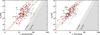Fig. 8

Correlation between the bulk Lorentz factor Γ₀ and the isotropic equivalent energy E_iso. Same symbols as Fig. 7.

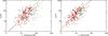Fig. 9

Correlation between the bulk Lorentz factor Γ₀ and the peak energy E_p. Same symbols as Fig. 7.

Table 4

Correlations between L_iso, E_iso, and E_p with Γ₀.

Figure 7 shows the correlation between Γ₀ (for the homogeneous and wind density circumburst medium, left and right panels, respectively) and L_iso. Lower limits $Γ_{0}^{LL}$ $\hbox{$\Gamma_{0}^{\rm LL}$}$ are shown by rightward black arrows and occupy the same region of the data points with estimated Γ₀ (red symbols). The green symbols show the LAT bursts which have the largest values of L_iso and Γ₀. Upper limits $Γ_{0}^{UL}$ $\hbox{$\Gamma_{0}^{\rm UL}$}$ obtained requiring that the onset of the afterglow happens after the main emission peak of the prompt light curve are shown by the grey (leftward) arrows.

The shadowed grey region shown in Fig. 7 shows the limit obtained requiring that the deceleration happens after the transparency radius, that is, R_dec ≥ R_th. Two different limits are shown corresponding to different (by a factor of 10) assumptions for R₀, that is, the radius where the jet is launched (see Eq. (16)). The correlation between L_iso and Γ₀ in the wind profile (bottom panel of Fig. 7) is less scattered than in the homogeneous case (upper panel of Fig. 7). The correlations between Γ₀ and the isotropic energy E_iso and the peak energy E_p are shown in Figs. 8 and 9, respectively. Symbols are the same as in Fig. 7. Also in these cases, the correlation in the wind case is less scattered than in the homogeneous case.

The correlations shown in Figs. 7–9 were analysed computing the Spearman’s rank correlation coefficient r and its probability P and fitting the data, with the bisector method, with a linear model: 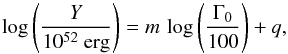$\log (\frac{Y}{10^{52} erg}) = m \log (\frac{Γ_{0}}{100}) + q,$ $\begin{equation} \log\left(\frac{Y}{10^{52} ~{\rm erg}}\right)=m\,\log\left(\frac{\Gamma_{0}}{100}\right)+q \label{norm1} , \end{equation}$ (17)where Y is either L_iso or E_iso. Similarly, for the correlation between E_p and Γ₀ we adopted the model: 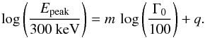$\log (\frac{E_{peak}}{300 keV}) = m \log (\frac{Γ_{0}}{100}) + q .$ $\begin{equation} \log\left(\frac{E_{\rm peak}}{300~ {\rm keV}}\right)=m\,\log\left(\frac{\Gamma_{0}}{100}\right)+q. \label{norm2} \end{equation}$ (18)The results are given in Table 4 both for the homogeneous and for the wind case. Correlation analysis considering only estimates of Γ₀ are shown by the red solid line in Figs. 7–9.

In order to reconstruct the correlation considering measured Γ₀ and upper/lower limits, we adopted the same Monte Carlo procedure described in Sect. 3. We generate 10⁵ samples composed by the GRBs with measured Γ₀ and assigning to the 85 GRBs without measured t_p a value of Γ₀ randomly extracted from the reconstructed distribution of Γ₀ shown in Fig. 6. We then analyse the correlations of Γ₀ and the energetic variables within these random samples and report the central values of the correlation parameters (coefficient, probability, slope and normalisation) in Table 4. In all cases we find significant correlations also when upper/lower limits are accounted for with this Monte Carlo method. The corresponding correlation lines are shown with the dot–dashed lines in Figs. 7–9. We note that the correlations found with only Γ₀ or reconstructed accounting also for limits are very similar.

Figure 7 (and similarly Figs. 8 and 9) shows that the planes are not uniformly filled with data points, contrary to what is claimed by Hascoët et al. (2014). Indeed, the right part of the planes of Figs. 7 and 8 corresponding to large Γ₀ and any possible value of L_iso and E_iso, respectively, are limited by the excluded region, that is, deceleration should happen after the fireball transparency. Moreover, the upper limits obtained requiring that the afterglow onset time t_p is after the main prompt emission peak leads to the upper limits shown by the grey downward arrows in Figs. 7 and 8, which are even more constraining than the shaded regions. This confirms that the bulk Lorentz factor is indeed strongly correlated with the prompt emission properties (E_iso, L_iso, and E_p).

Fig. 10

Distribution of comoving frame properties of GRBs. Left panel: comoving frame isotropic luminosity (back and grey histogram for the homogeneous and wind case, respectively) and of the isotropic energy (red and orange histogram for the homogeneous and wind case, respectively). Right panel: comoving frame peak energy (black and grey histogram for the homogeneous and wind case, respectively).

Table 5

Average values and width of the distribution of the (log values of) E_iso, L_iso, and E_p, in the rest frame and in the comoving frame (both for the homogeneous and the wind density profile).

We compute the comoving frame peak energy and isotropic energy with the equations derived in G12: $E_{peak}^{'} = 3 E_{peak} / 5 Γ_{0}$ $\hbox{$E_{\rm peak}^{\prime}=3E_{\rm peak}/5\Gamma_0$}$ and $E_{iso}^{'} = E_{iso} / Γ_{0}$ $\hbox{$E_{\rm iso}^{\prime}=E_{\rm iso}/\Gamma_0$}$ . The luminosity $L_{iso}^{'} = 3 L_{iso} / 4 Γ_{0}^{2}$ $\hbox{$L_{\rm iso}^{\prime}=3L_{\rm iso}/4\Gamma_{0}^{2}$}$ . Primed quantities refer to the comoving frame. For GRBs with a $t_{p}^{UL}$ $\hbox{$t_{\rm p}^{\rm UL}$}$ a lower limit $Γ_{0}^{LL}$ $\hbox{$\Gamma_{0}^{\rm LL}$}$ transforms into an upper limit on $L_{iso}^{'}$ $\hbox{$L'_{\rm iso}$}$ , $E_{iso}^{'}$ $\hbox{$E'_{\rm iso}$}$ , and $E_{p}^{'}$ $\hbox{$E'_{\rm p}$}$ . Vice versa, lower limits $t_{p}^{LL}$ $\hbox{$t_{\rm p}^{\rm LL}$}$ provide upper limits $Γ_{0}^{UL}$ $\hbox{$\Gamma_{0}^{\rm UL}$}$ which transform the rest frame observables into lower limits in the comoving frame. Through the Monte Carlo method adopted in the previous sections we derive the distributions of the comoving frame $E_{iso}^{'}$ $\hbox{$E'_{\rm iso}$}$ , $L_{iso}^{'}$ $\hbox{$L'_{\rm iso}$}$ , and $E_{p}^{'}$ $\hbox{$E'_{\rm p}$}$ ; these are shown in Fig. 10. The average values of Γ₀ for the homogeneous ISM is larger than that of the wind case. For this reason the distributions of the comoving frame quantities shown in Fig. 10 are slightly shifted in the two scenarios with the homogeneous case resulting in a slightly smaller average value of the comoving frame isotropic energy, luminosity, and peak energy. The average values of the comoving frame distributions shown in Fig. 10 are reported in Table 5.

8. Summary

The present work assembles the largest sample of t_p, by revising and expanding (to June 2016) the original sample of G12, and including upper limits $t_{p}^{UL}$ $\hbox{$t_{\rm p}^{\rm UL}$}$ corresponding to GRBs without a measured onset time. Our sample, presented in Table A.1, is composed of:

67 GRBs with measured t_p: 66 long and one short (GRB 090510). Eight t_p are measured from the GeV light curve.

106 long GRBs with an upper limit $t_{p}^{UL}$ $\hbox{$t_{\rm p}^{\rm UL}$}$ . These are GRBs detected in the optical or GeV band within one day and showing a decaying light curve. Five $t_{p}^{UL}$ $\hbox{$t_{\rm p}^{\rm UL}$}$ are measured from the GeV light curve.

An upper limit $t_{p}^{UL}$ $\hbox{$t_{\rm p}^{\rm UL}$}$ gives a lower limit $Γ_{0}^{LL}$ $\hbox{$\Gamma_{0}^{\rm LL}$}$ according to equations in Sect. 4. Accounting only for the most stringent upper limits, we consider only the 85 bursts with $t_{p}^{UL} ≲ 11 500$ $\hbox{$t_{\rm p}^{\rm UL} \lesssim11\,500$}$ s, corresponding to five times the maximum t_p among the 66 GRBs. Therefore, the final sample is composed of 151 GRBs: 66 long GRBs¹⁰ with t_p and 85 GRBs with $t_{p}^{UL}$ $\hbox{$t_{\rm p}^{\rm UL}$}$ .

The observable is t_p: Fig. 1 shows that the relative position of the cumulative distribution of t_p (red line) and of lower limits $t_{p}^{UL}$ $\hbox{$t_{\rm p}^{\rm UL}$}$ (dashed line) suggests the presence of a selection bias against the measurement of intermediate/small t_p values. The earliest t_p are provided by the few GRBs with an onset measured from the GeV light curve by the LAT on board Fermi.

We can extract more information from the sample of t_p if we use also upper limits $t_{p}^{UL}$ $\hbox{$t_{\rm p}^{\rm UL}$}$ . Statistical methods (e.g. Feigelson & Nelson 1985) allow us to reconstruct the distribution of an observable adopting measurements and upper limits, provided upper limits cover the same range of values of detections. This is our case as shown in Fig. 1. We adopt the Kaplan-Meier estimator to reconstruct the distribution of t_p of the population of long GRBs. We find that:

The reconstructed distribution of t_p (solid black line with yellow shaded region in Fig. 1) has median value ⟨ t_p ⟩ ~ 60 s extending from a few seconds (t_p from LAT) to relatively late t_p ~ 10³ s; in the rest frame, the average t_p/ (1 + z) is 20 s.

The t_p distribution is consistent with the cumulative distribution of T_p,γ (dot–dashed grey line in Fig. 1). T_p,γ is the time when the prompt emission light curve peaks.

The rest frame t_p/ (1 + z) is inversely correlated with E_iso, L_iso and E_p (Fig. 4). These correlations are statistically significant (Table 1).

Since $Γ_{0} \propto t_{p}^{- (3 - s) / (8 - 2 s)}$ $\hbox{$\Gamma_{0} \propto t_{\rm p} ^{-(3-s)/(8-2s)}$}$ , an upper limit on t_p provides a lower limit $Γ_{0}^{LL}$ $\hbox{$\Gamma_{0}^{\rm LL}$}$ . We combine Γ₀ and $Γ_{0}^{LL}$ $\hbox{$\Gamma_{0}^{\rm LL}$}$ finding that:

The reconstructed distribution of Γ₀ (solid black line and yellow shaded region in Fig. 6) has a median of ⟨ Γ₀ ⟩ = 320 and 155 in the homogeneous and wind case, respectively (Table 3).

Γ₀ values span two orders of magnitude from 20 to 1000 in the wind case (right panel in Fig. 6) and a slightly smaller range in the homogeneous case (left panel in Fig. 6).

The distribution of Γ₀ is consistent with the distribution of upper limits derived under the assumption that the afterglow peak is larger than the peak of the prompt emission (i.e. t_p>T_p,γ – dotted grey line in Fig. 6).

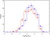Fig. 11

Distribution of the mass of the jet (in solar masses) for the homogeneous case (red solid line) and for the wind case (blue solid line) computed assuming a typical jet opening angle of 5 degrees.

Through a Monte Carlo method we combine the 66 t_p with the 85 GRBs with $t_{p}^{UL}$ $\hbox{$t_{\rm p}^{\rm UL}$}$ . In the latter cases Γ₀ should lie in the range $Γ_{0}^{LL} < Γ_{0} < Γ_{0}^{UL}$ $\hbox{$\Gamma_{0}^{\rm LL} < \Gamma_{0} < \Gamma_{0}^{\rm UL}$}$ (where $Γ_{0}^{LL}$ $\hbox{$\Gamma_{0}^{\rm LL}$}$ and $Γ_{0}^{UL}$ $\hbox{$\Gamma_{0}^{\rm UL}$}$ are obtained from $t_{p}^{UL}$ $\hbox{$t_{\rm p}^{\rm UL}$}$ and T_p,γ). We assign values of Γ₀, randomly extracted from the reconstructed distribution and requiring they are comprised within the above limits, to the 85 GRBs. Creating 10⁵ mock samples of 66 GRBs with measured Γ₀ plus the randomly assigned 85 values, we evaluate the various dependencies of this parameter on the prompt emission properties analysing these random samples:

There are significant correlations between Γ₀ and the prompt emission rest frame properties, namely E_iso, L_iso, and E_p (shown in Figs. 7, 8, and 10 and Table 4): $\begin{matrix} L_{iso} \propto Γ_{0, H}^{2.6} L_{iso} \propto Γ_{0, W}^{2.9}, \\ E_{iso} \propto Γ_{0, H}^{2.2} E_{iso} \propto Γ_{0, W}^{2.7}, \end{matrix}$ $\begin{eqnarray} &&L_{\rm iso}\propto \Gamma_{0,\rm H}^{2.6} \,\,\,\,\,\,\,\,\,\,\,\, L_{\rm iso}\propto \Gamma_{0,\rm W}^{2.9} ,\\ &&E_{\rm iso}\propto \Gamma_{0,\rm H}^{2.2} \,\,\,\,\,\,\,\,\,\,\,\, E_{\rm iso}\propto \Gamma_{0,\rm W}^{2.7} ,\\ &&E_{\rm p}\propto \Gamma_{0,\rm H}^{1.3} \,\,\,\,\,\,\,\,\,\,\,\, E_{\rm p}\propto \Gamma_{0,\rm W}^{1.4} \label{corre} , \end{eqnarray}$ where H and W denote the homogeneous and wind case, respectively. The correlations are less scattered in the W case.

The distribution of the data points and upper/lower limits in Figs. 7–9 show that these planes are not uniformly filled with data.

There is no correlation between the rest frame duration T₉₀/ (1 + z) and Γ₀.

With the distribution of bulk Lorentz factors reconstructed from our sample of GRBs, we can compute the baryon loading of the fireball M = E_k/ Γ₀c², where E_k = E_iso/η is the kinetic energy of the blast wave. This would lead to the isotropic equivalent mass loading but, since GRBs have a jet, we derive the baryon loading of the jet assuming a typical opening angle of 5 degrees (e.g. Ghirlanda et al. 2007). Figure 11 shows the distribution of the jet baryon loading in units of solar masses obtained in the homogeneous (red line) and wind (blue line) case. The baryon loading is distributed around a typical value of a few 10^-6M_⊙ which is similar in the two density scenarios.

9. Conclusions

We have extended the sample of GRBs with measured onset time t_p including for the first time also upper limits t_p. While the onset time happens relatively early (the mean value of the distribution, accounting for upper limits, is ~60 s in the observer frame), in most cases this happens after the time of the peak of the prompt emission of GRBs. This ensures that a considerable fraction of the fireball kinetic energy should have been transferred to the blast wave whose deceleration produces t_p. Therefore, the so called “thin shell approximation” (i.e. the requirement that most of the fireball energy has been transferred to the blast wave that decelerates into the interstellar medium) adopted in deriving Γ₀ from the measure of t_p holds. This regime is only partly established in jets that remain highly magnetised at the afterglow stage (Mimica et al. 2009) and seems to support a low magnetisation outflow. Moreover, we have shown that the synchrotron characteristic frequency ν_inj, computed at t_p, is above the optical R band (Fig. 5) for all bursts. This ensures that it cannot be responsible for the peak of the afterglow light curve sweeping through the observer frame optical band. This allows us to interpret t_p as the fireball deceleration onset time and use it to compute the bulk Lorentz factor Γ₀.

We have reviewed and compared the different methods and formulae proposed in the literature (Ghirlanda et al. 2012; Ghisellini et al. 2010; Molinari et al. 2007; Nappo et al. 2014; Nava et al. 2013; Sari & Piran 1999) to compute Γ₀ from t_p. They differ at most by a factor of two. Therefore, any different choice of the specific formula to compute Γ₀ should only introduce a small systematic difference in the derived correlation normalisation and average values.

The average Γ₀ is 320 and 155, for the homogeneous and wind cases, respectively. These values are larger than those found in G12 due to our larger sample (almost a factor 2) and to the inclusion of lower limits $Γ_{0}^{LL}$ $\hbox{$\Gamma_{0}^{\rm LL}$}$ . We confirm the existence of significant correlations between the GRB bulk Lorentz factor and the prompt emission observables, that is, isotropic energy and luminosity and peak energy (Eq. (21)). The Γ₀−L_iso, Γ₀−E_iso, and Γ₀−E_p correlations are not boundaries in these planes (opposite to what claimed by Hascoët et al. 2014). With respect to the sample considered in Hascoët et al. (2014), our samples of t_p and $t_{p}^{UL}$ $\hbox{$t_{\rm p}^{\rm UL}$}$ are a factor three and four larger, respectively.

By combining these correlations, we find $E_{p} \propto E_{iso}^{0.58}$ $\hbox{$E_{\rm p} \propto E_{\rm iso} ^{0.58}$}$ and $E_{p} \propto L_{iso}^{0.50}$ $\hbox{$E_{\rm p} \propto L_{\rm iso} ^{0.50}$}$ in the homogenous case (and $E_{p} \propto E_{iso}^{0.53}$ $\hbox{$E_{\rm p} \propto E_{\rm iso} ^{0.53}$}$ and $E_{p} \propto L_{iso}^{0.50}$ $\hbox{$E_{\rm p} \propto L_{\rm iso} ^{0.50}$}$ in the wind case). These slopes are consistent with the E_p−E_iso and E_p−L_iso correlations (Amati et al. 2002; Yonetoku et al. 2004) that we have re-derived here through our sample of 151 GRBs, and are $E_{p} \propto E_{iso}^{0.55 \pm 0.03}$ $\hbox{$E_{\rm p}\propto E_{\rm iso}^{0.55\pm0.03}$}$ and $E_{p} \propto L_{iso}^{0.53 \pm 0.03}$ $\hbox{$E_{\rm p}\propto L_{\rm iso}^{0.53\pm0.03}$}$ , respectively.

Finally, the knowledge of Γ₀ allows us to derive the mass of the fireball for individual GRBs. Assuming a typical jet opening angle of 5 degrees, the jet mass M_jet is similarly distributed for the homogeneous and wind cases (red and blue lines, respectively, in Fig. 11) between 10^-8 and 10^-4M_⊙.

¹

Liang et al. (2010), Lü et al. (2012) and Wu et al. (2011) include in their samples also bursts with a peak in the X-ray light curve thus resulting in a larger but less homogeneous and secure sample of t_p.

²

In these events Γ₀ might still be estimated, but only under some assumptions on the dynamical evolution of the burst outflow (e.g. GRB 090124 – Nappo et al. 2014).

³

The short GRB 090510 is not included in the distributions. Its onset time t_p = 0.2 s Ghirlanda et al. (2010) would place it in the lowest bin of the distribution.

⁴

We note also that for the LAT bursts (star symbols) the injection frequency is a factor 10 below the GeV band, and also in these cases the peak of the LAT light curve can be interpreted as the deceleration peak (Nava et al. 2017).

⁵

On the other hand, as discussed in G12 and Nappo et al. (2014), there are ways to obtain a peak also in the s = 2 case. This is why we consider both the homogeneous and the wind case for all bursts. Observationally, most early light curves indeed show a peak.

⁶

Liang et al. (2010) adopt the same equation as M07.

⁷

G10 derive t_peak in the case of an adiabatic or a fully radiative evolution of the fireball that propagates in a homogeneous medium. For our purposes we consider only the adiabatic case.

⁸

Although Eq. (7) is obtained with an incorrect normalisation of the relation between Γ and R, we report also this derivation since it was the first to propose a different method to derive the time of the peak of the afterglow. Cfr. with Eq. (8) showing the correct normalisation.

⁹

Changing the assumed value of R₀ within a factor of 10 shifts the green curve by a factor ~1.8.

¹⁰

In most of the Figures we show for comparison also the short GRB 090510: this is not included in the quantitive analysis.

Acknowledgments

INAF PRIN 2014 (1.05.01.94.12) is acknowledged. The anonymous referee is acknowledged for useful comments that helped to improve the content of the paper.

References

Abdo, A. A., Ackermann, M., Arimoto, M., et al. 2009a, Science, 323, 1688 [Google Scholar]
Abdo, A. A., Ackermann, M., Asano, K., et al. 2009b, ApJ, 707, 580 [NASA ADS] [CrossRef] [Google Scholar]
Ackermann, M., Ajello, M., Baldini, L., et al. 2010a, ApJ, 717, L127 [NASA ADS] [CrossRef] [Google Scholar]
Ackermann, M., Asano, K., Atwood, W. B., et al. 2010b, ApJ, 716, 1178 [NASA ADS] [CrossRef] [Google Scholar]
Ackermann, M., Ajello, M., Asano, K., et al. 2013, ApJS, 209, 11 [NASA ADS] [CrossRef] [Google Scholar]
Ackermann, M., Ajello, M., Asano, K., et al. 2014, Science, 343, 42 [NASA ADS] [CrossRef] [PubMed] [Google Scholar]
Akerlof, C. W., Kehoe, R. L., McKay, T. A., et al. 2003, PASP, 115, 132 [NASA ADS] [CrossRef] [Google Scholar]
Amati, L., Frontera, F., Tavani, M., et al. 2002, A&A, 390, 81 [NASA ADS] [CrossRef] [EDP Sciences] [Google Scholar]
Bardho, O., Gendre, B., Rossi, A., et al. 2016, MNRAS, 459, 508 [NASA ADS] [CrossRef] [Google Scholar]
Baring, M. G., & Harding, A. K. 1997, ApJ, 491, 663 [CrossRef] [Google Scholar]
Beniamini, P., & van der Horst, A. J. 2017, MNRAS, 472, 3161 [NASA ADS] [CrossRef] [Google Scholar]
Beniamini, P., Nava, L., Duran, R. B., & Piran, T. 2015, MNRAS, 454, 1073 [NASA ADS] [CrossRef] [Google Scholar]
Beniamini, P., Nava, L., & Piran, T. 2016, MNRAS, 461, 51 [NASA ADS] [CrossRef] [Google Scholar]
Berger, E., Kulkarni, S. R., Bloom, J. S., et al. 2002, ApJ, 581, 981 [NASA ADS] [CrossRef] [Google Scholar]
Bhalerao, V. B., Singer, L. P., Kasliwal, M. M., et al. 2014, GRB Coordinates Network, 16442 [Google Scholar]
Blandford, R. D., & McKee, C. F. 1976, Phys. Fluids, 19, 1130 [NASA ADS] [CrossRef] [Google Scholar]
Bloom, J. S., Perley, D. A., Li, W., et al. 2009, ApJ, 691, 723 [NASA ADS] [CrossRef] [PubMed] [Google Scholar]
Breeveld, A. A., & Kuin, N. P. M. 2013, GRB Coordinates Network, 14957 [Google Scholar]
Buckley, D., Potter, S., Kniazev, A., et al. 2014, GRB Coordinates Network, 17237 [Google Scholar]
Burd, A., Cwiok, M., Czyrkowski, H., et al. 2005, New Astron., 10, 409 [NASA ADS] [CrossRef] [Google Scholar]
Burgess, J. M., Bégué, D., Ryde, F., et al. 2016, ApJ, 822, 63 [NASA ADS] [CrossRef] [Google Scholar]
Butler, N. R., Kocevski, D., Bloom, J. S., & Curtis, J. L. 2007, ApJ, 671, 656 [NASA ADS] [CrossRef] [Google Scholar]
Butler, N. R., Bloom, J. S., & Poznanski, D. 2010, ApJ, 711, 495 [NASA ADS] [CrossRef] [Google Scholar]
Cenko, S. B., & Perley, D. A. 2015, GRB Coordinates Network, 17612 [Google Scholar]
Cenko, S. B., Urban, A. L., Perley, D. A., et al. 2015, ApJ, 803, L24 [NASA ADS] [CrossRef] [Google Scholar]
Covino, S., D’Avanzo, P., Klotz, A., et al. 2008, MNRAS, 388, 347 [NASA ADS] [CrossRef] [Google Scholar]
Cucchiara, A., Cenko, S. B., Bloom, J. S., et al. 2011, ApJ, 743, 154 [NASA ADS] [CrossRef] [Google Scholar]
Daigne, F., & Mochkovitch, R. 2002, MNRAS, 336, 1271 [NASA ADS] [CrossRef] [Google Scholar]
de Pasquale, M., & Cannizzo, J. K. 2013, GRB Coordinates Network, 14573 [Google Scholar]
Denisenko, D., Gorbovskoy, E., Lipunov, V., et al. 2012, GRB Coordinates Network, 13623 [Google Scholar]
Diercks, A. H., Deutsch, E. W., Castander, F. J., et al. 1998, ApJ, 503, L105 [NASA ADS] [CrossRef] [Google Scholar]
Feigelson, E. D., & Nelson, P. I. 1985, ApJ, 293, 192 [NASA ADS] [CrossRef] [Google Scholar]
Fenimore, E. E., Epstein, R. I., & Ho, C. 1993, A&AS, 97, 59 [NASA ADS] [Google Scholar]
Ferrero, A., Hanlon, L., Felletti, R., et al. 2010, Adv. Astron., 2010, 715237 [NASA ADS] [CrossRef] [Google Scholar]
Filgas, R., Greiner, J., Schady, P., et al. 2012, A&A, 546, A101 [NASA ADS] [CrossRef] [EDP Sciences] [Google Scholar]
Frail, D. A., Kulkarni, S. R., Nicastro, L., Feroci, M., & Taylor, G. B. 1997, Nature, 389, 261 [NASA ADS] [CrossRef] [Google Scholar]
Fukushima, T., To, S., Asano, K., & Fujita, Y. 2017, ApJ, 844, 92 [NASA ADS] [CrossRef] [Google Scholar]
Fynbo, J. U., Gorosabel, J., Dall, T. H., et al. 2001, A&A, 373, 796 [NASA ADS] [CrossRef] [EDP Sciences] [Google Scholar]
Galama, T. J., Briggs, M. S., Wijers, R. A. M. J., et al. 1999, Nature, 398, 394 [NASA ADS] [CrossRef] [Google Scholar]
Gendre, B., Klotz, A., Palazzi, E., et al. 2010, MNRAS, 405, 2372 [NASA ADS] [Google Scholar]
Genet, F., Daigne, F., & Mochkovitch, R. 2007, MNRAS, 381, 732 [NASA ADS] [CrossRef] [Google Scholar]
Ghirlanda, G., Nava, L., Ghisellini, G., & Firmani, C. 2007, A&A, 466, 127 [NASA ADS] [CrossRef] [EDP Sciences] [Google Scholar]
Ghirlanda, G., Ghisellini, G., & Nava, L. 2010, A&A, 510, L7 [NASA ADS] [CrossRef] [EDP Sciences] [Google Scholar]
Ghirlanda, G., Nava, L., Ghisellini, G., et al. 2012, MNRAS, 420, 483 [NASA ADS] [CrossRef] [Google Scholar]
Ghirlanda, G., Ghisellini, G., Salvaterra, R., et al. 2013a, MNRAS, 428, 1410 [NASA ADS] [CrossRef] [EDP Sciences] [Google Scholar]
Ghirlanda, G., Pescalli, A., & Ghisellini, G. 2013b, MNRAS, 432, 3237 [NASA ADS] [CrossRef] [Google Scholar]
Ghisellini, G., Ghirlanda, G., Nava, L., & Firmani, C. 2007, ApJ, 658, L75 [NASA ADS] [CrossRef] [Google Scholar]
Ghisellini, G., Nardini, M., Ghirlanda, G., & Celotti, A. 2009, MNRAS, 393, 253 [NASA ADS] [CrossRef] [Google Scholar]
Ghisellini, G., Ghirlanda, G., Nava, L., & Celotti, A. 2010, MNRAS, 403, 926 [NASA ADS] [CrossRef] [Google Scholar]
Goodman, J. 1986, ApJ, 308, L47 [NASA ADS] [CrossRef] [Google Scholar]
Gorbovskoy, E., Krushinski, V., Pruzhinskaya, M., et al. 2014a, GRB Coordinates Network, 16500 [Google Scholar]
Gorbovskoy, E., Lipunov, V., Kornilov, V., et al. 2014b, GRB Coordinates Network, 16307 [Google Scholar]
Gorbovskoy, E., Lipunov, V., Pruzhinskaya, M., et al. 2014c, GRB Coordinates Network, 15932 [Google Scholar]
Gorbovskoy, E. S., Lipunov, V. M., Buckley, D. A. H., et al. 2016, MNRAS, 455, 3312 [NASA ADS] [CrossRef] [Google Scholar]
Gorosabel, J., Mottola, S., de Ugarte Postigo, A., Hellmich, S., & Proffe, G. 2013, GRB Coordinates Network, 15469 [Google Scholar]
Gorosabel, J., Hellmich, S., de Ugarte Postigo, A., Mottola, S., & Thoene, C. 2014, GRB Coordinates Network, 17197 [Google Scholar]
Graff, P., Feroz, F., Hobson, M. P., & Lasenby, A. 2014, MNRAS, 441, 1741 [NASA ADS] [CrossRef] [Google Scholar]
Granot, J., & van der Horst, A. J. 2014, PASA, 31, e008 [NASA ADS] [CrossRef] [Google Scholar]
Greiner, J., Krühler, T., Fynbo, J. P. U., et al. 2009, ApJ, 693, 1610 [NASA ADS] [CrossRef] [Google Scholar]
Groot, P. J., Galama, T. J., Vreeswijk, P. M., et al. 1998, ApJ, 502, L123 [NASA ADS] [CrossRef] [Google Scholar]
Grupe, D., Brown, P. J., Cummings, J., et al. 2006, ApJ, 645, 464 [NASA ADS] [CrossRef] [Google Scholar]
Guidorzi, C., Steele, I. A., Melandri, A., et al. 2009, GRB Coordinates Network, 9375 [Google Scholar]
Halpern, J. P., Uglesich, R., Mirabal, N., et al. 2000, ApJ, 543, 697 [NASA ADS] [CrossRef] [Google Scholar]
Hascoët, R., Daigne, F., Mochkovitch, R., & Vennin, V. 2012, MNRAS, 421, 525 [NASA ADS] [Google Scholar]
Hascoët, R., Beloborodov, A. M., Daigne, F., & Mochkovitch, R. 2014, ApJ, 782, 5 [NASA ADS] [CrossRef] [Google Scholar]
Henden, A., Gross, J., Denny, B., Terrell, D., & Cooney, W. 2009, GRB Coordinates Network, 9211 [Google Scholar]
Holland, S., Fynbo, J. P. U., Hjorth, J., et al. 2001, A&A, 371, 52 [NASA ADS] [CrossRef] [EDP Sciences] [Google Scholar]
Holland, S. T., Soszyński, I., Gladders, M. D., et al. 2002, AJ, 124, 639 [NASA ADS] [CrossRef] [Google Scholar]
Ioka, K., Toma, K., Yamazaki, R., & Nakamura, T. 2006, A&A, 458, 7 [NASA ADS] [CrossRef] [EDP Sciences] [Google Scholar]
Isobe, T., Feigelson, E. D., & Nelson, P. I. 1986, ApJ, 306, 490 [NASA ADS] [CrossRef] [Google Scholar]
Isobe, T., Feigelson, E. D., Akritas, M. G., & Babu, G. J. 1990, ApJ, 364, 104 [NASA ADS] [CrossRef] [EDP Sciences] [Google Scholar]
Japelj, J., Kopac, D., Guidorzi, C., Mundell, C., & Virgili, F. 2012, GRB Coordinates Network, 14058 [Google Scholar]
Japelj, J., Kopač, D., Kobayashi, S., et al. 2014, ApJ, 785, 84 [NASA ADS] [CrossRef] [Google Scholar]
Jin, Z.-P., Covino, S., Della Valle, M., et al. 2013, ApJ, 774, 114 [NASA ADS] [CrossRef] [Google Scholar]
Kasliwal, M. M., Cenko, S. B., & Singer, L. P. 2014, GRB Coordinates Network, 16425 [Google Scholar]
King, O. G., Blinov, D., Giannios, D., et al. 2014, MNRAS, 445, L114 [NASA ADS] [CrossRef] [Google Scholar]
Kinugasa, K., & Torii, K. 2004, GRB Coordinates Network, 2832 [Google Scholar]
Klotz, A., Boër, M., Atteia, J. L., & Gendre, B. 2009, AJ, 137, 4100 [NASA ADS] [CrossRef] [Google Scholar]
Klotz, A., Turpin, D., Atteia, J. L., et al. 2016, GRB Coordinates Network, 19622 [Google Scholar]
Krimm, H. A., Granot, J., Marshall, F. E., et al. 2007, ApJ, 665, 554 [NASA ADS] [CrossRef] [Google Scholar]
Krolik, J. H., & Pier, E. A. 1991, ApJ, 373, 277 [NASA ADS] [CrossRef] [Google Scholar]
Kruehler, T., Malesani, D., Xu, D., et al. 2014, GRB Coordinates Network, 15899 [Google Scholar]
Krühler, T., Ledoux, C., Fynbo, J. P. U., et al. 2013, A&A, 557, A18 [NASA ADS] [CrossRef] [EDP Sciences] [Google Scholar]
Kuin, N. P. M., & Yershov, V. N. 2012, GRB Coordinates Network, 13808 [Google Scholar]
Kuin, P., de Pasquale, M., Malesani, D., & Brown, P. 2015, GRB Coordinates Network, 18224 [Google Scholar]
Kumar, P., & Barniol Duran, R. 2010, MNRAS, 409, 226 [NASA ADS] [CrossRef] [Google Scholar]
Kumar, P., & Zhang, B. 2015, Phys. Rep., 561, 1 [NASA ADS] [CrossRef] [Google Scholar]
Lacluyze, A., Haislip, J., Ivarsen, K., et al. 2011, GRB Coordinates Network, 12535 [Google Scholar]
Laskar, T., Alexander, K. D., Berger, E., et al. 2016, ApJ, 833, 88 [NASA ADS] [CrossRef] [Google Scholar]
Lei, W.-H., Zhang, B., & Liang, E.-W. 2013, ApJ, 765, 125 [NASA ADS] [CrossRef] [Google Scholar]
Li, W., Filippenko, A. V., Chornock, R., & Jha, S. 2003, ApJ, 586, L9 [NASA ADS] [CrossRef] [Google Scholar]
Liang, E.-W., Yi, S.-X., Zhang, J., et al. 2010, ApJ, 725, 2209 [NASA ADS] [CrossRef] [Google Scholar]
Liang, E.-W., Li, L., Gao, H., et al. 2013, ApJ, 774, 13 [Google Scholar]
Lien, A. Y., Barthelmy, S., Maselli, A., & Oates, S. R. 2014, GCN Report, 466 [Google Scholar]
Lipunov, V. M., Krylov, A. V., Kornilov, V. G., et al. 2004, Astron. Nachr., 325, 580 [NASA ADS] [CrossRef] [Google Scholar]
Lipunov, V. M., Gorosabel, J., Pruzhinskaya, M. V., et al. 2016, MNRAS, 455, 712 [NASA ADS] [CrossRef] [Google Scholar]
Lithwick, Y., & Sari, R. 2001, ApJ, 555, 540 [NASA ADS] [CrossRef] [Google Scholar]
Liu, B., Chen, W., Liang, Y.-F., et al. 2014, ApJ, 787, L6 [NASA ADS] [CrossRef] [Google Scholar]
Lü, J., Zou, Y.-C., Lei, W.-H., et al. 2012, ApJ, 751, 49 [NASA ADS] [CrossRef] [Google Scholar]
Maiorano, E., Masetti, N., Palazzi, E., et al. 2006, A&A, 455, 423 [NASA ADS] [CrossRef] [EDP Sciences] [Google Scholar]
Margutti, R., Guidorzi, C., Chincarini, G., et al. 2010, MNRAS, 406, 2149 [NASA ADS] [CrossRef] [Google Scholar]
Marshall, F. E., & Cannizzo, J. K. 2015, GRB Coordinates Network, 17820 [Google Scholar]
Marshall, F. E., vanden Berk, D. E., & Racusin, J. 2007, GRB Coordinates Network, 6041 [Google Scholar]
Martin-Carrillo, A., Hanlon, L., Topinka, M., et al. 2014, A&A, 567, A84 [NASA ADS] [CrossRef] [EDP Sciences] [Google Scholar]
Mazaeva, E., Klunko, E., Volnova, A., Korobtsev, I., & Pozanenko, A. 2015, GRB Coordinates Network, 18175 [Google Scholar]
Melandri, A., Kobayashi, S., Mundell, C. G., et al. 2010, ApJ, 723, 1331 [NASA ADS] [CrossRef] [Google Scholar]
Melandri, A., Covino, S., Rogantini, D., et al. 2014a, A&A, 565, A72 [NASA ADS] [CrossRef] [EDP Sciences] [Google Scholar]
Melandri, A., Virgili, F. J., Guidorzi, C., et al. 2014b, A&A, 572, A55 [NASA ADS] [CrossRef] [EDP Sciences] [Google Scholar]
Mesler, R. A., Pihlström, Y. M., Taylor, G. B., & Granot, J. 2012, ApJ, 759, 4 [NASA ADS] [CrossRef] [Google Scholar]
Mimica, P., Giannios, D., & Aloy, M. A. 2009, A&A, 494, 879 [NASA ADS] [CrossRef] [EDP Sciences] [Google Scholar]
Molinari, E., Vergani, S. D., Malesani, D., et al. 2007, A&A, 469, L13 [NASA ADS] [CrossRef] [EDP Sciences] [Google Scholar]
Nappo, F., Ghisellini, G., Ghirlanda, G., et al. 2014, MNRAS, 445, 1625 [NASA ADS] [CrossRef] [Google Scholar]
Nardini, M., Ghisellini, G., Ghirlanda, G., & Celotti, A. 2010, MNRAS, 403, 1131 [NASA ADS] [CrossRef] [Google Scholar]
Nardini, M., Elliott, J., Filgas, R., et al. 2014, A&A, 562, A29 [NASA ADS] [CrossRef] [EDP Sciences] [Google Scholar]
Nava, L., Sironi, L., Ghisellini, G., Celotti, A., & Ghirlanda, G. 2013, MNRAS, 433, 2107 [NASA ADS] [CrossRef] [Google Scholar]
Nava, L., Vianello, G., Omodei, N., et al. 2014, MNRAS, 443, 3578 [NASA ADS] [CrossRef] [Google Scholar]
Nava, L., Desiante, R., Longo, F., et al. 2017, MNRAS, 465, 811 [NASA ADS] [CrossRef] [Google Scholar]
Oates, S. R., & Hagen, L. M. Z. 2015, GRB Coordinates Network, 17424 [Google Scholar]
Oates, S. R., & Racusin, J. L. 2012, GRB Coordinates Network, 13725 [Google Scholar]
Paczynski, B. 1986, ApJ, 308, L43 [NASA ADS] [CrossRef] [Google Scholar]
Page, K. L., Starling, R. L. C., Fitzpatrick, G., et al. 2011, MNRAS, 416, 2078 [NASA ADS] [CrossRef] [Google Scholar]
Panaitescu, A. 2008, MNRAS, 383, 1143 [NASA ADS] [CrossRef] [Google Scholar]
Panaitescu, A. 2017, ApJ, 837, 13 [NASA ADS] [CrossRef] [Google Scholar]
Panaitescu, A., & Kumar, P. 2000, ApJ, 543, 66 [NASA ADS] [CrossRef] [Google Scholar]
Park, H. S., Ables, E., Band, D. L., et al. 1997, ApJ, 490, 99 [NASA ADS] [CrossRef] [Google Scholar]
Perley, D. A., Bloom, J. S., Butler, N. R., et al. 2008a, ApJ, 672, 449 [NASA ADS] [CrossRef] [Google Scholar]
Perley, D. A., Li, W., Chornock, R., et al. 2008b, ApJ, 688, 470 [NASA ADS] [CrossRef] [Google Scholar]
Pihlström, Y. M., Taylor, G. B., Granot, J., & Doeleman, S. 2007, ApJ, 664, 411 [NASA ADS] [CrossRef] [Google Scholar]
Piran, T. 1999, Phys. Rep., 314, 575 [NASA ADS] [CrossRef] [Google Scholar]
Price, P. A., Kulkarni, S. R., Berger, E., et al. 2003, ApJ, 589, 838 [NASA ADS] [CrossRef] [Google Scholar]
Racusin, J. L., Karpov, S. V., Sokolowski, M., et al. 2008, Nature, 455, 183 [Google Scholar]
Romano, P., Campana, S., Chincarini, G., et al. 2006, A&A, 456, 917 [NASA ADS] [CrossRef] [EDP Sciences] [Google Scholar]
Rossi, A., Schulze, S., Klose, S., et al. 2011, A&A, 529, A142 [NASA ADS] [CrossRef] [EDP Sciences] [Google Scholar]
Rykoff, E. S., Aharonian, F., Akerlof, C. W., et al. 2009, ApJ, 702, 489 [NASA ADS] [CrossRef] [Google Scholar]
Sahu, K. C., Vreeswijk, P., Bakos, G., et al. 2000, ApJ, 540, 74 [NASA ADS] [CrossRef] [Google Scholar]
Sakamoto, T., Barthelmy, S. D., Baumgartner, W. H., et al. 2011, ApJS, 195, 2 [NASA ADS] [CrossRef] [Google Scholar]
Salvaterra, R., Della Valle, M., Campana, S., et al. 2009, Nature, 461, 1258 [NASA ADS] [CrossRef] [PubMed] [Google Scholar]
Salvaterra, R., Campana, S., Vergani, S. D., et al. 2012, ApJ, 749, 68 [NASA ADS] [CrossRef] [Google Scholar]
Sánchez-Ramírez, R., Hancock, P. J., Jóhannesson, G., et al. 2017, MNRAS, 464, 4624 [NASA ADS] [CrossRef] [Google Scholar]
Santana, R., Barniol Duran, R., & Kumar, P. 2014, ApJ, 785, 29 [NASA ADS] [CrossRef] [Google Scholar]
Sari, R., & Piran, T. 1999, ApJ, 520, 641 [NASA ADS] [CrossRef] [Google Scholar]
Sari, R., Piran, T., & Narayan, R. 1998, ApJ, 497, L17 [NASA ADS] [CrossRef] [Google Scholar]
Sato, R., Kawai, N., Suzuki, M., et al. 2003, ApJ, 599, L9 [NASA ADS] [CrossRef] [Google Scholar]
Siegel, M. H., & Gompertz, B. P. 2014, GRB Coordinates Network, 16219 [Google Scholar]
Singer, L. P., Cenko, S. B., Kasliwal, M. M., Fremling, C., & Dzigan, Y. 2014, GRB Coordinates Network, 16226 [Google Scholar]
Soderberg, A. M., Kulkarni, S. R., Price, P. A., et al. 2006, ApJ, 636, 391 [NASA ADS] [CrossRef] [Google Scholar]
Stanek, K. Z., Garnavich, P. M., Kaluzny, J., Pych, W., & Thompson, I. 1999, ApJ, 522, L39 [NASA ADS] [CrossRef] [Google Scholar]
Stanek, K. Z., Garnavich, P. M., Jha, S., et al. 2001, ApJ, 563, 592 [NASA ADS] [CrossRef] [Google Scholar]
Steele, I. A., Mundell, C. G., Smith, R. J., Kobayashi, S., & Guidorzi, C. 2009, Nature, 462, 767 [NASA ADS] [CrossRef] [PubMed] [Google Scholar]
Still, M., Roming, P. W. A., Mason, K. O., et al. 2005, ApJ, 635, 1187 [NASA ADS] [CrossRef] [Google Scholar]
Tang, Q.-W., Peng, F.-K., Wang, X.-Y., & Tam, P.-H. T. 2015, ApJ, 806, 194 [NASA ADS] [CrossRef] [Google Scholar]
Taylor, G. B., Frail, D. A., Berger, E., & Kulkarni, S. R. 2004, ApJ, 609, L1 [NASA ADS] [CrossRef] [Google Scholar]
Taylor, G. B., Momjian, E., Pihlström, Y., Ghosh, T., & Salter, C. 2005, ApJ, 622, 986 [NASA ADS] [CrossRef] [Google Scholar]
Thöne, C. C., Kann, D. A., Jóhannesson, G., et al. 2010, A&A, 523, A70 [NASA ADS] [CrossRef] [EDP Sciences] [Google Scholar]
Toma, K., Ioka, K., Yamazaki, R., & Nakamura, T. 2006, ApJ, 640, L139 [NASA ADS] [CrossRef] [Google Scholar]
Trotter, A., Frank, N., Lacluyze, A., et al. 2013a, GRB Coordinates Network, 14375 [Google Scholar]
Trotter, A., Frank, N., Lacluyze, A., et al. 2013b, GRB Coordinates Network, 14427 [Google Scholar]
Trotter, A., Reichart, D., Haislip, J., et al. 2013c, GRB Coordinates Network, 15491 [Google Scholar]
Trotter, A., Lacluyze, A., Haislip, J., et al. 2014, GRB Coordinates Network, 16304 [Google Scholar]
Trotter, A., Reichart, D., Haislip, J., et al. 2015, GRB Coordinates Network, 18472 [Google Scholar]
Urata, Y., Tashiro, M. S., Tamagawa, T., et al. 2011, PASJ, 63, 137 [NASA ADS] [CrossRef] [Google Scholar]
Veres, P., Corsi, A., Frail, D. A., Cenko, S. B., & Perley, D. A. 2015, ApJ, 810, 31 [NASA ADS] [CrossRef] [Google Scholar]
Vestrand, W. T., Borozdin, K. N., Brumby, S. P., et al. 2002, in Advanced Global Communications Technologies for Astronomy II, ed. R. I. Kibrick, Proc. SPIE, 4845, 126 [NASA ADS] [CrossRef] [Google Scholar]
Virgili, F. J., Mundell, C. G., & Melandri, A. 2013, GRB Coordinates Network, 14785 [Google Scholar]
Volnova, A., Pozanenko, A., Mundrzyjewski, W., & Tereshenko, V. 2014, GRB Coordinates Network, 16809 [Google Scholar]
Waxman, E. 1997, ApJ, 491, L19 [NASA ADS] [CrossRef] [Google Scholar]
Williams, G. G., Blake, C., & Hartmann, D. 2002, GRB Coordinates Network, 1492 [Google Scholar]
Wren, J., Vestrand, W. T., Wozniak, P., & Davis, H. 2012, GRB Coordinates Network, 14013 [Google Scholar]
Wu, Q., Zou, Y.-C., Cao, X., Wang, D.-X., & Chen, L. 2011, ApJ, 740, L21 [NASA ADS] [CrossRef] [Google Scholar]
Yonetoku, D., Murakami, T., Nakamura, T., et al. 2004, ApJ, 609, 935 [NASA ADS] [CrossRef] [Google Scholar]
Yost, S. A., Alatalo, K., Rykoff, E. S., et al. 2006, ApJ, 636, 959 [NASA ADS] [CrossRef] [Google Scholar]
Yost, S. A., Swan, H. F., Rykoff, E. S., et al. 2007, ApJ, 657, 925 [NASA ADS] [CrossRef] [Google Scholar]
Zaninoni, E., Bernardini, M. G., Margutti, R., Oates, S., & Chincarini, G. 2013, A&A, 557, A12 [NASA ADS] [CrossRef] [EDP Sciences] [Google Scholar]
Zerbi, R. M., Chincarini, G., Ghisellini, G., et al. 2001, Astron. Nachr., 322, 275 [NASA ADS] [CrossRef] [Google Scholar]
Zhang, B.-B., van Eerten, H., Burrows, D. N., et al. 2015, ApJ, 806, 15 [NASA ADS] [CrossRef] [Google Scholar]
Zhang, Q., Huang, Y. F., & Zong, H. S. 2016, ApJ, 823, 156 [NASA ADS] [CrossRef] [Google Scholar]
Zhao, X.-H., Li, Z., & Bai, J.-M. 2011, ApJ, 726, 89 [NASA ADS] [CrossRef] [Google Scholar]
Zheng, W., & Filippenko, A. V. 2015, GRB Coordinates Network, 17585 [Google Scholar]
Zheng, W., Flewelling, H., Guver, T., & Yuan, F. 2013, GRB Coordinates Network, 14208 [Google Scholar]
Zheng, W., Filippenko, A. V., Morgan, A., & Cenko, S. B. 2014a, GRB Coordinates Network, 16137 [Google Scholar]
Zheng, W., Filippenko, A. V., Morgan, A., & Cenko, S. B. 2014b, GRB Coordinates Network, 16156 [Google Scholar]
Zou, Y.-C., & Piran, T. 2010, MNRAS, 402, 1854 [NASA ADS] [CrossRef] [Google Scholar]
Zou, Y.-C., Fan, Y.-Z., & Piran, T. 2011, ApJ, 726, L2 [NASA ADS] [CrossRef] [Google Scholar]

Appendix A: Additional table

Table A.1

Sample of GRBs with measured t_p (69 events) from the peak of the light curve (those from the LAT light curve are labelled “L”).

All Tables

Table 1

Correlation between rest frame t_p/ (1 + z) and prompt emission properties (Fig. 4).

In the text

Table 2

Comparison between the different methods of estimating Γ₀ found in literature.

In the text

Table 3

Average values and 68% confidence intervals on Γ₀ (derived with only measured t_p – red line in Fig. 6) or including lower limits $Γ_{0}^{LL}$ $\hbox{$\Gamma_{0}^{\rm LL}$}$ (derived from upper limits $t_{p}^{UL}$ $\hbox{$t_{\rm p}^{\rm UL}$}$ – black line in Fig. 6).

In the text

Table 4

Correlations between L_iso, E_iso, and E_p with Γ₀.

In the text

Table 5

Average values and width of the distribution of the (log values of) E_iso, L_iso, and E_p, in the rest frame and in the comoving frame (both for the homogeneous and the wind density profile).

In the text

Table A.1

Sample of GRBs with measured t_p (69 events) from the peak of the light curve (those from the LAT light curve are labelled “L”).

In the text

All Figures

Fig. 1

Cumulative distribution of the afterglow onset time t_p (red solid line) in the observer frame for the 66 long GRBs of the “Gold+Silver” sample. The black dashed line (marked with leftward arrows) is the cumulative distribution of 85 upper limits on t_p (filtered from Table A.1 according to $t_{p}^{UL} \leq 5 \times \max (t_{p}) ~ 11 500$ $\hbox{$t_{\rm p}^{\rm UL}\le 5\times \max(t_{\rm p})\sim11\,500$}$ s). The black solid line (shaded yellow region) is the reconstructed t_p distribution (95% confidence interval) accounting for $t_{p}^{UL}$ $\hbox{$t_{\rm p}^{\rm UL}$}$ through the Kaplan Meier estimator. The dotted and dot–dashed lines are the cumulative distributions of T₉₀ and T_p,γ (i.e. the time of the peak of the prompt emission light curve), respectively, for the 151 long GRBs. The distributions have been normalised to the respective sample size. Insert: Distribution of t_p (solid blue line) and of upper limits $t_{p}^{UL}$ $\hbox{$t_{\rm p}^{\rm UL}$}$ (dashed cyan line with leftward arrows) of the 50 GRBs of our sample (16 with t_p and 34 with $t_{p}^{UL}$ $\hbox{$t_{\rm p}^{\rm UL}$}$ ) also present in the Swift BAT complete sample (Salvaterra et al. 2012).

In the text

	Fig. 2 Cumulative distribution of the afterglow onset time t_p in the rest frame. Same symbols and colour code as in Fig. 1.
In the text

Fig. 3

Top panel: GRB duration T₉₀ vs. afterglow peak time t_p. GRBs with measured t_p are shown with red circles (green stars for LAT bursts). Upper limits on t_p are shown by the black arrows (green arrows for LAT GRBs). Bottom panel: time of the peak of the prompt emission light curve T_p,γ vs. t_p. Same symbols and colours as in the top panel. In both panels the equality is shown by the dashed line and the short GRB 090510 is shown by the green square.

In the text

	Fig. 4 Left panel: t_p/ (1 + z) vs. E_iso. GRBs with estimates of t_p are shown with filled red circles (green symbols for LAT events). Upper limits on t_p (Table A.1) are shown by the black arrows (green arrows for LAT events). Middle panel: t_p/ (1 + z) vs. L_iso. Right panel: t_p/ (1 + z) vs. E_p. In all panels the short GRB 090510 is shown by the green square symbol.
In the text

Fig. 5

Injection frequency at the t_p for each GRB. The optical-R frequency is show by the horizontal line. The injection frequency is shown for the homogeneous and wind case with red and blue symbols. GRBs with t_p from the LAT light curve are shown with star symbols. The scaling t^{− 3/2} of the injection frequency is shown for reference (it is not a fit) by the dashed line. Vertical bars, shown only for the red symbols, represent the position of the injection frequency obtained assuming ϵ_B in the range 10^-4−10^-1.

In the text

Fig. 6

Cumulative distribution of Γ₀ for GRBs with measured t_p (red solid line). The distribution of lower limits $Γ_{0}^{LL}$ $\hbox{$\Gamma_{0}^{\rm LL}$}$ , derived for GRBs with an upper limit on the onset time $t_{p}^{UL}$ $\hbox{$t_{\rm p}^{\rm UL}$}$ , is shown by the dashed black curve (with rightward arrows). Assuming t_p ≥ T_p,γ the distribution of upper limits on Γ₀ is shown by the dotted grey line (with leftward arrows). The most stringent limit on the distribution of Γ₀ is shown by the green solid line which assumes that deceleration radius R_dec ≥ R(τ = 1), that is, the transparency radius (Eq. (16)). Joining estimates of Γ₀ and lower limits $Γ_{0}^{LL}$ $\hbox{$\Gamma_{0}^{\rm LL}$}$ the reconstructed (through the KM estimator) distribution of Γ₀ is shown by the solid black line (and its 95% uncertainty by the yellow shaded region). The distributions are normalised to their respective number of elements. The two panels (right and left, respectively) show the case of a homogeneous (s = 0) and wind (s = 2) medium.

In the text

Fig. 7

Correlation between the isotropic equivalent luminosity L_iso and the bulk Lorentz factor Γ₀. Estimates of Γ₀ from the measured afterglow onset t_p for 68 long GRBs (red filled circles and green filled stars) and the short GRB 090510 (green filled square symbol). Lower limits $Γ_{0}^{LL}$ $\hbox{$\Gamma_{0}^{\rm LL}$}$ (derived from upper limits on the onset time $t_{p}^{UL}$ $\hbox{$t_{\rm p}^{\rm UL}$}$ ) are shown by the rightward black arrows. Upper limits $Γ_{0}^{UL}$ $\hbox{$\Gamma_{0}^{\rm UL}$}$ (derived assuming that the afterglow onset time is larger than the peak time of the prompt emission, that is, t_p ≥ T_p,γ) are shown by the grey (leftward) arrows. Upper limit on Γ₀ imposed by the requirement that the deceleration radius is larger than the transparency radius is shown by the grey shaded triangular region (for two values of the radius R₀ where the fireball is formed – see Eq. (16)). The solid red line shows the correlation obtained with Γ₀ solely (bisector method), while the black dot–dashed line is the correlation obtained through the Monte Carlo method which accounts for the reconstructed distribution of Γ₀. Left and right panels show the case of a homogeneous and wind medium, respectively.

In the text

	Fig. 8 Correlation between the bulk Lorentz factor Γ₀ and the isotropic equivalent energy E_iso. Same symbols as Fig. 7.
In the text

	Fig. 9 Correlation between the bulk Lorentz factor Γ₀ and the peak energy E_p. Same symbols as Fig. 7.
In the text

Fig. 10

Distribution of comoving frame properties of GRBs. Left panel: comoving frame isotropic luminosity (back and grey histogram for the homogeneous and wind case, respectively) and of the isotropic energy (red and orange histogram for the homogeneous and wind case, respectively). Right panel: comoving frame peak energy (black and grey histogram for the homogeneous and wind case, respectively).

In the text

	Fig. 11 Distribution of the mass of the jet (in solar masses) for the homogeneous case (red solid line) and for the wind case (blue solid line) computed assuming a typical jet opening angle of 5 degrees.
In the text

Current usage metrics show cumulative count of Article Views (full-text article views including HTML views, PDF and ePub downloads, according to the available data) and Abstracts Views on Vision4Press platform.

Data correspond to usage on the plateform after 2015. The current usage metrics is available 48-96 hours after online publication and is updated daily on week days.

Initial download of the metrics may take a while.

[1] Abdo, A. A., Ackermann, M., Arimoto, M., et al. 2009a, Science, 323, 1688 [Google Scholar]

[2] Abdo, A. A., Ackermann, M., Asano, K., et al. 2009b, ApJ, 707, 580 [NASA ADS] [CrossRef] [Google Scholar]

[3] Ackermann, M., Ajello, M., Baldini, L., et al. 2010a, ApJ, 717, L127 [NASA ADS] [CrossRef] [Google Scholar]

[4] Ackermann, M., Asano, K., Atwood, W. B., et al. 2010b, ApJ, 716, 1178 [NASA ADS] [CrossRef] [Google Scholar]

[5] Ackermann, M., Ajello, M., Asano, K., et al. 2013, ApJS, 209, 11 [NASA ADS] [CrossRef] [Google Scholar]

[6] Ackermann, M., Ajello, M., Asano, K., et al. 2014, Science, 343, 42 [NASA ADS] [CrossRef] [PubMed] [Google Scholar]

[7] Akerlof, C. W., Kehoe, R. L., McKay, T. A., et al. 2003, PASP, 115, 132 [NASA ADS] [CrossRef] [Google Scholar]

[8] Amati, L., Frontera, F., Tavani, M., et al. 2002, A&A, 390, 81 [NASA ADS] [CrossRef] [EDP Sciences] [Google Scholar]

[9] Bardho, O., Gendre, B., Rossi, A., et al. 2016, MNRAS, 459, 508 [NASA ADS] [CrossRef] [Google Scholar]

[10] Baring, M. G., & Harding, A. K. 1997, ApJ, 491, 663 [CrossRef] [Google Scholar]

[11] Beniamini, P., & van der Horst, A. J. 2017, MNRAS, 472, 3161 [NASA ADS] [CrossRef] [Google Scholar]

[12] Beniamini, P., Nava, L., Duran, R. B., & Piran, T. 2015, MNRAS, 454, 1073 [NASA ADS] [CrossRef] [Google Scholar]

[13] Beniamini, P., Nava, L., & Piran, T. 2016, MNRAS, 461, 51 [NASA ADS] [CrossRef] [Google Scholar]

[14] Berger, E., Kulkarni, S. R., Bloom, J. S., et al. 2002, ApJ, 581, 981 [NASA ADS] [CrossRef] [Google Scholar]

[15] Bhalerao, V. B., Singer, L. P., Kasliwal, M. M., et al. 2014, GRB Coordinates Network, 16442 [Google Scholar]

[16] Blandford, R. D., & McKee, C. F. 1976, Phys. Fluids, 19, 1130 [NASA ADS] [CrossRef] [Google Scholar]

[17] Bloom, J. S., Perley, D. A., Li, W., et al. 2009, ApJ, 691, 723 [NASA ADS] [CrossRef] [PubMed] [Google Scholar]

[18] Breeveld, A. A., & Kuin, N. P. M. 2013, GRB Coordinates Network, 14957 [Google Scholar]

[19] Buckley, D., Potter, S., Kniazev, A., et al. 2014, GRB Coordinates Network, 17237 [Google Scholar]

[20] Burd, A., Cwiok, M., Czyrkowski, H., et al. 2005, New Astron., 10, 409 [NASA ADS] [CrossRef] [Google Scholar]

[21] Burgess, J. M., Bégué, D., Ryde, F., et al. 2016, ApJ, 822, 63 [NASA ADS] [CrossRef] [Google Scholar]

[22] Butler, N. R., Kocevski, D., Bloom, J. S., & Curtis, J. L. 2007, ApJ, 671, 656 [NASA ADS] [CrossRef] [Google Scholar]

[23] Butler, N. R., Bloom, J. S., & Poznanski, D. 2010, ApJ, 711, 495 [NASA ADS] [CrossRef] [Google Scholar]

[24] Cenko, S. B., & Perley, D. A. 2015, GRB Coordinates Network, 17612 [Google Scholar]

[25] Cenko, S. B., Urban, A. L., Perley, D. A., et al. 2015, ApJ, 803, L24 [NASA ADS] [CrossRef] [Google Scholar]

[26] Covino, S., D’Avanzo, P., Klotz, A., et al. 2008, MNRAS, 388, 347 [NASA ADS] [CrossRef] [Google Scholar]

[27] Cucchiara, A., Cenko, S. B., Bloom, J. S., et al. 2011, ApJ, 743, 154 [NASA ADS] [CrossRef] [Google Scholar]

[28] Daigne, F., & Mochkovitch, R. 2002, MNRAS, 336, 1271 [NASA ADS] [CrossRef] [Google Scholar]

[29] de Pasquale, M., & Cannizzo, J. K. 2013, GRB Coordinates Network, 14573 [Google Scholar]

[30] Denisenko, D., Gorbovskoy, E., Lipunov, V., et al. 2012, GRB Coordinates Network, 13623 [Google Scholar]

[31] Diercks, A. H., Deutsch, E. W., Castander, F. J., et al. 1998, ApJ, 503, L105 [NASA ADS] [CrossRef] [Google Scholar]

[32] Feigelson, E. D., & Nelson, P. I. 1985, ApJ, 293, 192 [NASA ADS] [CrossRef] [Google Scholar]

[33] Fenimore, E. E., Epstein, R. I., & Ho, C. 1993, A&AS, 97, 59 [NASA ADS] [Google Scholar]

[34] Ferrero, A., Hanlon, L., Felletti, R., et al. 2010, Adv. Astron., 2010, 715237 [NASA ADS] [CrossRef] [Google Scholar]

[35] Filgas, R., Greiner, J., Schady, P., et al. 2012, A&A, 546, A101 [NASA ADS] [CrossRef] [EDP Sciences] [Google Scholar]

[36] Frail, D. A., Kulkarni, S. R., Nicastro, L., Feroci, M., & Taylor, G. B. 1997, Nature, 389, 261 [NASA ADS] [CrossRef] [Google Scholar]

[37] Fukushima, T., To, S., Asano, K., & Fujita, Y. 2017, ApJ, 844, 92 [NASA ADS] [CrossRef] [Google Scholar]

[38] Fynbo, J. U., Gorosabel, J., Dall, T. H., et al. 2001, A&A, 373, 796 [NASA ADS] [CrossRef] [EDP Sciences] [Google Scholar]

[39] Galama, T. J., Briggs, M. S., Wijers, R. A. M. J., et al. 1999, Nature, 398, 394 [NASA ADS] [CrossRef] [Google Scholar]

[40] Gendre, B., Klotz, A., Palazzi, E., et al. 2010, MNRAS, 405, 2372 [NASA ADS] [Google Scholar]

[41] Genet, F., Daigne, F., & Mochkovitch, R. 2007, MNRAS, 381, 732 [NASA ADS] [CrossRef] [Google Scholar]

[42] Ghirlanda, G., Nava, L., Ghisellini, G., & Firmani, C. 2007, A&A, 466, 127 [NASA ADS] [CrossRef] [EDP Sciences] [Google Scholar]

[43] Ghirlanda, G., Ghisellini, G., & Nava, L. 2010, A&A, 510, L7 [NASA ADS] [CrossRef] [EDP Sciences] [Google Scholar]

[44] Ghirlanda, G., Nava, L., Ghisellini, G., et al. 2012, MNRAS, 420, 483 [NASA ADS] [CrossRef] [Google Scholar]

[45] Ghirlanda, G., Ghisellini, G., Salvaterra, R., et al. 2013a, MNRAS, 428, 1410 [NASA ADS] [CrossRef] [EDP Sciences] [Google Scholar]

[46] Ghirlanda, G., Pescalli, A., & Ghisellini, G. 2013b, MNRAS, 432, 3237 [NASA ADS] [CrossRef] [Google Scholar]

[47] Ghisellini, G., Ghirlanda, G., Nava, L., & Firmani, C. 2007, ApJ, 658, L75 [NASA ADS] [CrossRef] [Google Scholar]

[48] Ghisellini, G., Nardini, M., Ghirlanda, G., & Celotti, A. 2009, MNRAS, 393, 253 [NASA ADS] [CrossRef] [Google Scholar]

[49] Ghisellini, G., Ghirlanda, G., Nava, L., & Celotti, A. 2010, MNRAS, 403, 926 [NASA ADS] [CrossRef] [Google Scholar]

[50] Goodman, J. 1986, ApJ, 308, L47 [NASA ADS] [CrossRef] [Google Scholar]

[51] Gorbovskoy, E., Krushinski, V., Pruzhinskaya, M., et al. 2014a, GRB Coordinates Network, 16500 [Google Scholar]

[52] Gorbovskoy, E., Lipunov, V., Kornilov, V., et al. 2014b, GRB Coordinates Network, 16307 [Google Scholar]

[53] Gorbovskoy, E., Lipunov, V., Pruzhinskaya, M., et al. 2014c, GRB Coordinates Network, 15932 [Google Scholar]

[54] Gorbovskoy, E. S., Lipunov, V. M., Buckley, D. A. H., et al. 2016, MNRAS, 455, 3312 [NASA ADS] [CrossRef] [Google Scholar]

[55] Gorosabel, J., Mottola, S., de Ugarte Postigo, A., Hellmich, S., & Proffe, G. 2013, GRB Coordinates Network, 15469 [Google Scholar]

[56] Gorosabel, J., Hellmich, S., de Ugarte Postigo, A., Mottola, S., & Thoene, C. 2014, GRB Coordinates Network, 17197 [Google Scholar]

[57] Graff, P., Feroz, F., Hobson, M. P., & Lasenby, A. 2014, MNRAS, 441, 1741 [NASA ADS] [CrossRef] [Google Scholar]

[58] Granot, J., & van der Horst, A. J. 2014, PASA, 31, e008 [NASA ADS] [CrossRef] [Google Scholar]

[59] Greiner, J., Krühler, T., Fynbo, J. P. U., et al. 2009, ApJ, 693, 1610 [NASA ADS] [CrossRef] [Google Scholar]

[60] Groot, P. J., Galama, T. J., Vreeswijk, P. M., et al. 1998, ApJ, 502, L123 [NASA ADS] [CrossRef] [Google Scholar]

[61] Grupe, D., Brown, P. J., Cummings, J., et al. 2006, ApJ, 645, 464 [NASA ADS] [CrossRef] [Google Scholar]

[62] Guidorzi, C., Steele, I. A., Melandri, A., et al. 2009, GRB Coordinates Network, 9375 [Google Scholar]

[63] Halpern, J. P., Uglesich, R., Mirabal, N., et al. 2000, ApJ, 543, 697 [NASA ADS] [CrossRef] [Google Scholar]

[64] Hascoët, R., Daigne, F., Mochkovitch, R., & Vennin, V. 2012, MNRAS, 421, 525 [NASA ADS] [Google Scholar]

[65] Hascoët, R., Beloborodov, A. M., Daigne, F., & Mochkovitch, R. 2014, ApJ, 782, 5 [NASA ADS] [CrossRef] [Google Scholar]

[66] Henden, A., Gross, J., Denny, B., Terrell, D., & Cooney, W. 2009, GRB Coordinates Network, 9211 [Google Scholar]

[67] Holland, S., Fynbo, J. P. U., Hjorth, J., et al. 2001, A&A, 371, 52 [NASA ADS] [CrossRef] [EDP Sciences] [Google Scholar]

[68] Holland, S. T., Soszyński, I., Gladders, M. D., et al. 2002, AJ, 124, 639 [NASA ADS] [CrossRef] [Google Scholar]

[69] Ioka, K., Toma, K., Yamazaki, R., & Nakamura, T. 2006, A&A, 458, 7 [NASA ADS] [CrossRef] [EDP Sciences] [Google Scholar]

[70] Isobe, T., Feigelson, E. D., & Nelson, P. I. 1986, ApJ, 306, 490 [NASA ADS] [CrossRef] [Google Scholar]

[71] Isobe, T., Feigelson, E. D., Akritas, M. G., & Babu, G. J. 1990, ApJ, 364, 104 [NASA ADS] [CrossRef] [EDP Sciences] [Google Scholar]

[72] Japelj, J., Kopac, D., Guidorzi, C., Mundell, C., & Virgili, F. 2012, GRB Coordinates Network, 14058 [Google Scholar]

[73] Japelj, J., Kopač, D., Kobayashi, S., et al. 2014, ApJ, 785, 84 [NASA ADS] [CrossRef] [Google Scholar]

[74] Jin, Z.-P., Covino, S., Della Valle, M., et al. 2013, ApJ, 774, 114 [NASA ADS] [CrossRef] [Google Scholar]

[75] Kasliwal, M. M., Cenko, S. B., & Singer, L. P. 2014, GRB Coordinates Network, 16425 [Google Scholar]

[76] King, O. G., Blinov, D., Giannios, D., et al. 2014, MNRAS, 445, L114 [NASA ADS] [CrossRef] [Google Scholar]

[77] Kinugasa, K., & Torii, K. 2004, GRB Coordinates Network, 2832 [Google Scholar]

[78] Klotz, A., Boër, M., Atteia, J. L., & Gendre, B. 2009, AJ, 137, 4100 [NASA ADS] [CrossRef] [Google Scholar]

[79] Klotz, A., Turpin, D., Atteia, J. L., et al. 2016, GRB Coordinates Network, 19622 [Google Scholar]

[80] Krimm, H. A., Granot, J., Marshall, F. E., et al. 2007, ApJ, 665, 554 [NASA ADS] [CrossRef] [Google Scholar]

[81] Krolik, J. H., & Pier, E. A. 1991, ApJ, 373, 277 [NASA ADS] [CrossRef] [Google Scholar]

[82] Kruehler, T., Malesani, D., Xu, D., et al. 2014, GRB Coordinates Network, 15899 [Google Scholar]

[83] Krühler, T., Ledoux, C., Fynbo, J. P. U., et al. 2013, A&A, 557, A18 [NASA ADS] [CrossRef] [EDP Sciences] [Google Scholar]

[84] Kuin, N. P. M., & Yershov, V. N. 2012, GRB Coordinates Network, 13808 [Google Scholar]

[85] Kuin, P., de Pasquale, M., Malesani, D., & Brown, P. 2015, GRB Coordinates Network, 18224 [Google Scholar]

[86] Kumar, P., & Barniol Duran, R. 2010, MNRAS, 409, 226 [NASA ADS] [CrossRef] [Google Scholar]

[87] Kumar, P., & Zhang, B. 2015, Phys. Rep., 561, 1 [NASA ADS] [CrossRef] [Google Scholar]

[88] Lacluyze, A., Haislip, J., Ivarsen, K., et al. 2011, GRB Coordinates Network, 12535 [Google Scholar]

[89] Laskar, T., Alexander, K. D., Berger, E., et al. 2016, ApJ, 833, 88 [NASA ADS] [CrossRef] [Google Scholar]

[90] Lei, W.-H., Zhang, B., & Liang, E.-W. 2013, ApJ, 765, 125 [NASA ADS] [CrossRef] [Google Scholar]

[91] Li, W., Filippenko, A. V., Chornock, R., & Jha, S. 2003, ApJ, 586, L9 [NASA ADS] [CrossRef] [Google Scholar]

[92] Liang, E.-W., Yi, S.-X., Zhang, J., et al. 2010, ApJ, 725, 2209 [NASA ADS] [CrossRef] [Google Scholar]

[93] Liang, E.-W., Li, L., Gao, H., et al. 2013, ApJ, 774, 13 [Google Scholar]

[94] Lien, A. Y., Barthelmy, S., Maselli, A., & Oates, S. R. 2014, GCN Report, 466 [Google Scholar]

[95] Lipunov, V. M., Krylov, A. V., Kornilov, V. G., et al. 2004, Astron. Nachr., 325, 580 [NASA ADS] [CrossRef] [Google Scholar]

[96] Lipunov, V. M., Gorosabel, J., Pruzhinskaya, M. V., et al. 2016, MNRAS, 455, 712 [NASA ADS] [CrossRef] [Google Scholar]

[97] Lithwick, Y., & Sari, R. 2001, ApJ, 555, 540 [NASA ADS] [CrossRef] [Google Scholar]

[98] Liu, B., Chen, W., Liang, Y.-F., et al. 2014, ApJ, 787, L6 [NASA ADS] [CrossRef] [Google Scholar]

[99] Lü, J., Zou, Y.-C., Lei, W.-H., et al. 2012, ApJ, 751, 49 [NASA ADS] [CrossRef] [Google Scholar]

[100] Maiorano, E., Masetti, N., Palazzi, E., et al. 2006, A&A, 455, 423 [NASA ADS] [CrossRef] [EDP Sciences] [Google Scholar]

[101] Margutti, R., Guidorzi, C., Chincarini, G., et al. 2010, MNRAS, 406, 2149 [NASA ADS] [CrossRef] [Google Scholar]

[102] Marshall, F. E., & Cannizzo, J. K. 2015, GRB Coordinates Network, 17820 [Google Scholar]

[103] Marshall, F. E., vanden Berk, D. E., & Racusin, J. 2007, GRB Coordinates Network, 6041 [Google Scholar]

[104] Martin-Carrillo, A., Hanlon, L., Topinka, M., et al. 2014, A&A, 567, A84 [NASA ADS] [CrossRef] [EDP Sciences] [Google Scholar]

[105] Mazaeva, E., Klunko, E., Volnova, A., Korobtsev, I., & Pozanenko, A. 2015, GRB Coordinates Network, 18175 [Google Scholar]

[106] Melandri, A., Kobayashi, S., Mundell, C. G., et al. 2010, ApJ, 723, 1331 [NASA ADS] [CrossRef] [Google Scholar]

[107] Melandri, A., Covino, S., Rogantini, D., et al. 2014a, A&A, 565, A72 [NASA ADS] [CrossRef] [EDP Sciences] [Google Scholar]

[108] Melandri, A., Virgili, F. J., Guidorzi, C., et al. 2014b, A&A, 572, A55 [NASA ADS] [CrossRef] [EDP Sciences] [Google Scholar]

[109] Mesler, R. A., Pihlström, Y. M., Taylor, G. B., & Granot, J. 2012, ApJ, 759, 4 [NASA ADS] [CrossRef] [Google Scholar]

[110] Mimica, P., Giannios, D., & Aloy, M. A. 2009, A&A, 494, 879 [NASA ADS] [CrossRef] [EDP Sciences] [Google Scholar]

[111] Molinari, E., Vergani, S. D., Malesani, D., et al. 2007, A&A, 469, L13 [NASA ADS] [CrossRef] [EDP Sciences] [Google Scholar]

[112] Nappo, F., Ghisellini, G., Ghirlanda, G., et al. 2014, MNRAS, 445, 1625 [NASA ADS] [CrossRef] [Google Scholar]

[113] Nardini, M., Ghisellini, G., Ghirlanda, G., & Celotti, A. 2010, MNRAS, 403, 1131 [NASA ADS] [CrossRef] [Google Scholar]

[114] Nardini, M., Elliott, J., Filgas, R., et al. 2014, A&A, 562, A29 [NASA ADS] [CrossRef] [EDP Sciences] [Google Scholar]

[115] Nava, L., Sironi, L., Ghisellini, G., Celotti, A., & Ghirlanda, G. 2013, MNRAS, 433, 2107 [NASA ADS] [CrossRef] [Google Scholar]

[116] Nava, L., Vianello, G., Omodei, N., et al. 2014, MNRAS, 443, 3578 [NASA ADS] [CrossRef] [Google Scholar]

[117] Nava, L., Desiante, R., Longo, F., et al. 2017, MNRAS, 465, 811 [NASA ADS] [CrossRef] [Google Scholar]

[118] Oates, S. R., & Hagen, L. M. Z. 2015, GRB Coordinates Network, 17424 [Google Scholar]

[119] Oates, S. R., & Racusin, J. L. 2012, GRB Coordinates Network, 13725 [Google Scholar]

[120] Paczynski, B. 1986, ApJ, 308, L43 [NASA ADS] [CrossRef] [Google Scholar]

[121] Page, K. L., Starling, R. L. C., Fitzpatrick, G., et al. 2011, MNRAS, 416, 2078 [NASA ADS] [CrossRef] [Google Scholar]

[122] Panaitescu, A. 2008, MNRAS, 383, 1143 [NASA ADS] [CrossRef] [Google Scholar]

[123] Panaitescu, A. 2017, ApJ, 837, 13 [NASA ADS] [CrossRef] [Google Scholar]

[124] Panaitescu, A., & Kumar, P. 2000, ApJ, 543, 66 [NASA ADS] [CrossRef] [Google Scholar]

[125] Park, H. S., Ables, E., Band, D. L., et al. 1997, ApJ, 490, 99 [NASA ADS] [CrossRef] [Google Scholar]

[126] Perley, D. A., Bloom, J. S., Butler, N. R., et al. 2008a, ApJ, 672, 449 [NASA ADS] [CrossRef] [Google Scholar]

[127] Perley, D. A., Li, W., Chornock, R., et al. 2008b, ApJ, 688, 470 [NASA ADS] [CrossRef] [Google Scholar]

[128] Pihlström, Y. M., Taylor, G. B., Granot, J., & Doeleman, S. 2007, ApJ, 664, 411 [NASA ADS] [CrossRef] [Google Scholar]

[129] Piran, T. 1999, Phys. Rep., 314, 575 [NASA ADS] [CrossRef] [Google Scholar]

[130] Price, P. A., Kulkarni, S. R., Berger, E., et al. 2003, ApJ, 589, 838 [NASA ADS] [CrossRef] [Google Scholar]

[131] Racusin, J. L., Karpov, S. V., Sokolowski, M., et al. 2008, Nature, 455, 183 [Google Scholar]

[132] Romano, P., Campana, S., Chincarini, G., et al. 2006, A&A, 456, 917 [NASA ADS] [CrossRef] [EDP Sciences] [Google Scholar]

[133] Rossi, A., Schulze, S., Klose, S., et al. 2011, A&A, 529, A142 [NASA ADS] [CrossRef] [EDP Sciences] [Google Scholar]

[134] Rykoff, E. S., Aharonian, F., Akerlof, C. W., et al. 2009, ApJ, 702, 489 [NASA ADS] [CrossRef] [Google Scholar]

[135] Sahu, K. C., Vreeswijk, P., Bakos, G., et al. 2000, ApJ, 540, 74 [NASA ADS] [CrossRef] [Google Scholar]

[136] Sakamoto, T., Barthelmy, S. D., Baumgartner, W. H., et al. 2011, ApJS, 195, 2 [NASA ADS] [CrossRef] [Google Scholar]

[137] Salvaterra, R., Della Valle, M., Campana, S., et al. 2009, Nature, 461, 1258 [NASA ADS] [CrossRef] [PubMed] [Google Scholar]

[138] Salvaterra, R., Campana, S., Vergani, S. D., et al. 2012, ApJ, 749, 68 [NASA ADS] [CrossRef] [Google Scholar]

[139] Sánchez-Ramírez, R., Hancock, P. J., Jóhannesson, G., et al. 2017, MNRAS, 464, 4624 [NASA ADS] [CrossRef] [Google Scholar]

[140] Santana, R., Barniol Duran, R., & Kumar, P. 2014, ApJ, 785, 29 [NASA ADS] [CrossRef] [Google Scholar]

[141] Sari, R., & Piran, T. 1999, ApJ, 520, 641 [NASA ADS] [CrossRef] [Google Scholar]

[142] Sari, R., Piran, T., & Narayan, R. 1998, ApJ, 497, L17 [NASA ADS] [CrossRef] [Google Scholar]

[143] Sato, R., Kawai, N., Suzuki, M., et al. 2003, ApJ, 599, L9 [NASA ADS] [CrossRef] [Google Scholar]

[144] Siegel, M. H., & Gompertz, B. P. 2014, GRB Coordinates Network, 16219 [Google Scholar]

[145] Singer, L. P., Cenko, S. B., Kasliwal, M. M., Fremling, C., & Dzigan, Y. 2014, GRB Coordinates Network, 16226 [Google Scholar]

[146] Soderberg, A. M., Kulkarni, S. R., Price, P. A., et al. 2006, ApJ, 636, 391 [NASA ADS] [CrossRef] [Google Scholar]

[147] Stanek, K. Z., Garnavich, P. M., Kaluzny, J., Pych, W., & Thompson, I. 1999, ApJ, 522, L39 [NASA ADS] [CrossRef] [Google Scholar]

[148] Stanek, K. Z., Garnavich, P. M., Jha, S., et al. 2001, ApJ, 563, 592 [NASA ADS] [CrossRef] [Google Scholar]

[149] Steele, I. A., Mundell, C. G., Smith, R. J., Kobayashi, S., & Guidorzi, C. 2009, Nature, 462, 767 [NASA ADS] [CrossRef] [PubMed] [Google Scholar]

[150] Still, M., Roming, P. W. A., Mason, K. O., et al. 2005, ApJ, 635, 1187 [NASA ADS] [CrossRef] [Google Scholar]

[151] Tang, Q.-W., Peng, F.-K., Wang, X.-Y., & Tam, P.-H. T. 2015, ApJ, 806, 194 [NASA ADS] [CrossRef] [Google Scholar]

[152] Taylor, G. B., Frail, D. A., Berger, E., & Kulkarni, S. R. 2004, ApJ, 609, L1 [NASA ADS] [CrossRef] [Google Scholar]

[153] Taylor, G. B., Momjian, E., Pihlström, Y., Ghosh, T., & Salter, C. 2005, ApJ, 622, 986 [NASA ADS] [CrossRef] [Google Scholar]

[154] Thöne, C. C., Kann, D. A., Jóhannesson, G., et al. 2010, A&A, 523, A70 [NASA ADS] [CrossRef] [EDP Sciences] [Google Scholar]

[155] Toma, K., Ioka, K., Yamazaki, R., & Nakamura, T. 2006, ApJ, 640, L139 [NASA ADS] [CrossRef] [Google Scholar]

[156] Trotter, A., Frank, N., Lacluyze, A., et al. 2013a, GRB Coordinates Network, 14375 [Google Scholar]

[157] Trotter, A., Frank, N., Lacluyze, A., et al. 2013b, GRB Coordinates Network, 14427 [Google Scholar]

[158] Trotter, A., Reichart, D., Haislip, J., et al. 2013c, GRB Coordinates Network, 15491 [Google Scholar]

[159] Trotter, A., Lacluyze, A., Haislip, J., et al. 2014, GRB Coordinates Network, 16304 [Google Scholar]

[160] Trotter, A., Reichart, D., Haislip, J., et al. 2015, GRB Coordinates Network, 18472 [Google Scholar]

[161] Urata, Y., Tashiro, M. S., Tamagawa, T., et al. 2011, PASJ, 63, 137 [NASA ADS] [CrossRef] [Google Scholar]

[162] Veres, P., Corsi, A., Frail, D. A., Cenko, S. B., & Perley, D. A. 2015, ApJ, 810, 31 [NASA ADS] [CrossRef] [Google Scholar]

[163] Vestrand, W. T., Borozdin, K. N., Brumby, S. P., et al. 2002, in Advanced Global Communications Technologies for Astronomy II, ed. R. I. Kibrick, Proc. SPIE, 4845, 126 [NASA ADS] [CrossRef] [Google Scholar]

[164] Virgili, F. J., Mundell, C. G., & Melandri, A. 2013, GRB Coordinates Network, 14785 [Google Scholar]

[165] Volnova, A., Pozanenko, A., Mundrzyjewski, W., & Tereshenko, V. 2014, GRB Coordinates Network, 16809 [Google Scholar]

[166] Waxman, E. 1997, ApJ, 491, L19 [NASA ADS] [CrossRef] [Google Scholar]

[167] Williams, G. G., Blake, C., & Hartmann, D. 2002, GRB Coordinates Network, 1492 [Google Scholar]

[168] Wren, J., Vestrand, W. T., Wozniak, P., & Davis, H. 2012, GRB Coordinates Network, 14013 [Google Scholar]

[169] Wu, Q., Zou, Y.-C., Cao, X., Wang, D.-X., & Chen, L. 2011, ApJ, 740, L21 [NASA ADS] [CrossRef] [Google Scholar]

[170] Yonetoku, D., Murakami, T., Nakamura, T., et al. 2004, ApJ, 609, 935 [NASA ADS] [CrossRef] [Google Scholar]

[171] Yost, S. A., Alatalo, K., Rykoff, E. S., et al. 2006, ApJ, 636, 959 [NASA ADS] [CrossRef] [Google Scholar]

[172] Yost, S. A., Swan, H. F., Rykoff, E. S., et al. 2007, ApJ, 657, 925 [NASA ADS] [CrossRef] [Google Scholar]

[173] Zaninoni, E., Bernardini, M. G., Margutti, R., Oates, S., & Chincarini, G. 2013, A&A, 557, A12 [NASA ADS] [CrossRef] [EDP Sciences] [Google Scholar]

[174] Zerbi, R. M., Chincarini, G., Ghisellini, G., et al. 2001, Astron. Nachr., 322, 275 [NASA ADS] [CrossRef] [Google Scholar]

[175] Zhang, B.-B., van Eerten, H., Burrows, D. N., et al. 2015, ApJ, 806, 15 [NASA ADS] [CrossRef] [Google Scholar]

[176] Zhang, Q., Huang, Y. F., & Zong, H. S. 2016, ApJ, 823, 156 [NASA ADS] [CrossRef] [Google Scholar]

[177] Zhao, X.-H., Li, Z., & Bai, J.-M. 2011, ApJ, 726, 89 [NASA ADS] [CrossRef] [Google Scholar]

[178] Zheng, W., & Filippenko, A. V. 2015, GRB Coordinates Network, 17585 [Google Scholar]

[179] Zheng, W., Flewelling, H., Guver, T., & Yuan, F. 2013, GRB Coordinates Network, 14208 [Google Scholar]

[180] Zheng, W., Filippenko, A. V., Morgan, A., & Cenko, S. B. 2014a, GRB Coordinates Network, 16137 [Google Scholar]

[181] Zheng, W., Filippenko, A. V., Morgan, A., & Cenko, S. B. 2014b, GRB Coordinates Network, 16156 [Google Scholar]

[182] Zou, Y.-C., & Piran, T. 2010, MNRAS, 402, 1854 [NASA ADS] [CrossRef] [Google Scholar]

[183] Zou, Y.-C., Fan, Y.-Z., & Piran, T. 2011, ApJ, 726, L2 [NASA ADS] [CrossRef] [Google Scholar]

Bulk Lorentz factors of gamma-ray bursts

1. Introduction

2. The sample

2.1. Afterglow onset tp

2.1.1. The gold sample

2.1.2. The silver sample

2.2. Upper limits on tp

3. Sample properties

3.1. Distribution of the observer frame tp

3.2. Distribution of the rest frame tp

3.3. Comparison between tp, T90, and Tp,γ

3.4. Empirical correlations

4. On the origin of the afterglow peak time tp

5. Estimate of Γ0

5.1. Sari & Piran (1999)

5.2. Molinari et al. (2007)

5.3. Ghisellini et al. (2010)

5.4. Ghirlanda et al. (2012)

5.5. Nava et al. (2013)

5.6. Nappo et al. (2014)

5.7. Comparison between different methods

6. Results

6.1. Distribution of Γ0

7. Correlations

8. Summary

9. Conclusions

Acknowledgments

References

Appendix A: Additional table

All Tables

All Figures

2.1. Afterglow onset t_p

2.2. Upper limits on t_p

3.1. Distribution of the observer frame t_p

3.2. Distribution of the rest frame t_p

3.3. Comparison between t_p, T₉₀, and T_p,γ

4. On the origin of the afterglow peak time t_p

5. Estimate of Γ₀

6.1. Distribution of Γ₀