| Issue |
A&A
Volume 609, January 2018
|
|
|---|---|---|
| Article Number | A7 | |
| Number of page(s) | 26 | |
| Section | Galactic structure, stellar clusters and populations | |
| DOI | https://doi.org/10.1051/0004-6361/201731093 | |
| Published online | 22 December 2017 | |
Stellar population of the superbubble N 206 in the LMC
I. Analysis of the Of-type stars
1 Institut für Physik und Astronomie, Universität Potsdam, Karl-Liebknecht-Str. 24/25, 14476 Potsdam, Germany
e-mail: This email address is being protected from spambots. You need JavaScript enabled to view it.
2 Department of Astronomy, University of Wisconsin – Madison, WI 53706, USA
Received: 3 May 2017
Accepted: 28 August 2017
Abstract
Context. Massive stars severely influence their environment by their strong ionizing radiation and by the momentum and kinetic energy input provided by their stellar winds and supernovae. Quantitative analyses of massive stars are required to understand how their feedback creates and shapes large scale structures of the interstellar medium. The giant H ii region N 206 in the Large Magellanic Cloud contains an OB association that powers a superbubble filled with hot X-ray emitting gas, serving as an ideal laboratory in this context.
Aims. We aim to estimate stellar and wind parameters of all OB stars in N 206 by means of quantitative spectroscopic analyses. In this first paper, we focus on the nine Of-type stars located in this region. We determine their ionizing flux and wind mechanical energy. The analysis of nitrogen abundances in our sample probes rotational mixing.
Methods. We obtained optical spectra with the multi-object spectrograph FLAMES at the ESO-VLT. When possible, the optical spectroscopy was complemented by UV spectra from the HST, IUE, and FUSE archives. Detailed spectral classifications are presented for our sample Of-type stars. For the quantitative spectroscopic analysis we used the Potsdam Wolf-Rayet model atmosphere code. We determined the physical parameters and nitrogen abundances of our sample stars by fitting synthetic spectra to the observations.
Results. The stellar and wind parameters of nine Of-type stars, which are largely derived from spectral analysis are used to construct wind momentum − luminosity relationship. We find that our sample follows a relation close to the theoretical prediction, assuming clumped winds. The most massive star in the N 206 association is an Of supergiant that has a very high mass-loss rate. Two objects in our sample reveal composite spectra, showing that the Of primaries have companions of late O subtype. All stars in our sample have an evolutionary age of less than 4 million yr, with the O2-type star being the youngest. All these stars show a systematic discrepancy between evolutionary and spectroscopic masses. All stars in our sample are nitrogen enriched. Nitrogen enrichment shows a clear correlation with increasing projected rotational velocities.
Conclusions. The mechanical energy input from the Of stars alone is comparable to the energy stored in the N 206 superbubble as measured from the observed X-ray and Hα emission.
Key words: stars: early-type / Magellanic Clouds / stars: atmospheres / stars: winds, outflows / stars: mass-loss / stars: massive
© ESO, 2017
1. Introduction
Superbubbles filled by hot, ~ 1 MK, gas are the large scale structures with characteristic size ~ 100 pc in the interstellar medium (ISM; Mac Low & McCray 1988). Superbubbles provide direct evidence for the energy feedback from massive star clusters or OB associations to the ISM. With a distance modulus of only DM = 18.5 mag (Madore & Freedman 1998; Pietrzyński et al. 2013), the Large Magellanic Cloud (LMC) provides a good platform for detailed spectroscopy of massive stars in superbubbles. Additionally, its face-on aspect and low interstellar extinction make it an excellent laboratory to study feedback. With an observed metallicity of approximately [Fe/H] = −0.31 ± 0.04 or 0.5 Z⊙ (Rolleston et al. 2002), the LMC exhibits a very different history of star formation compared to the Milky Way. Several massive star-forming regions in the LMC, especially 30 Doradus and the associated stellar populations have been extensively studied by many authors (e.g., Evans et al. 2011; Ramírez-Agudelo et al. 2017). In this paper we present the study of the Of-type stars in the massive star-forming region N 206.
N 206 (alias LHA 120-N 206 or DEM L 221) is a giant H ii region in the south-east of the LMC that is energized by the young cluster NGC 2018 (see Fig. 1) and two OB associations, LH 66 and LH 69. Imaging studies with HST, Spitzer, and WISE in the optical and infrared (IR) have already unveiled the spatial structure of the NGC 2018/N 206 region (Gorjian et al. 2004; Romita et al. 2010). This complex contains a superbubble observed as a source of diffuse X-rays, and a supernova remnant. The current star formation in N 206 is taking place at the rim of the X-ray superbubble (Gruendl & Chu 2009). The X-ray emission in N 206 region has been studied by Kavanagh et al. (2012) using observations obtained by the XMM-Newton X-ray telescope. However, the study of feedback was constrained by the lack of detailed knowledge on its massive star population.
To obtain a census of young massive stars in N 206 complex and study their feedback we conducted a spectroscopic survey of all blue stars with mV< 16 mag with the FLAMES multi-object spectrograph at ESO’s Very Large Telescope (VLT). Our total sample comprises 164 OB-type stars. The inspection and classification of the spectra revealed that nine objects belong to the Of subclass (Walborn et al. 2002) and comprise the hottest stars in our whole sample. The present paper focuses on the spectral analysis of these Of-type stars, while the subsequent paper (Paper II) will cover the detailed analyses of the entire OB star population, along with a detailed investigation of the energy feedback in this region.
The spectroscopic observations and spectral classifications are presented in Sect. 2. Section 3 describes the quantitative analyses of these stellar spectra using Potsdam Wolf-Rayet (PoWR) atmosphere models. Section 4 presents the results and discussions. The final Sect. 5 provides a summary and general conclusions. The appendices encompass comments on the individual objects (Appendix A) and the spectral fits of the analyzed Of stars (Appendix B).
2. Spectroscopy
We observed the complete massive star population associated with the N 206 superbubble on 2015 December 19–20 with VLT-FLAMES. In the Medusa-fiber mode, FLAMES (Pasquini et al. 2002) can simultaneously record the spectra of up to 132 targets. Each fiber has an aperture of 1.2″ radius. The nine Of stars are a subsample of this larger survey. The observation was carried out using three of the standard settings of the Giraffe spectrograph LR02 (resolving power R = 6000, 3960–4567 Å), LR03 (R = 7500, 4501–5071 Å), and HR15N (R = 19 200, 6442–6817 Å), respectively. We took three to six exposures (30 min each) for each pointing in three spectrograph setting to improve the S/N. The higher resolution at Hα is utilized to determine stellar wind parameters and to distinguish nebular emission from the stellar lines.
The ESO Common Pipeline Library1 FLAMES reduction routines were executed for the standard processing stages such as bias subtraction, flat fielding, and wavelength calibration. We used the ESO data file organizer GASGANO2 for organizing and inspecting the VLT data and to execute the data reduction tasks. The obtained spectra are not flux calibrated. Multi-exposures were normalized and median combined to get the final spectra without cosmic rays in each settings. The spectra were rectified by fitting the stellar continuum with a piece-wise linear function. Finally, for each star, the LR02 and LR03 spectra were merged to form the medium resolution blue spectra from 3960 to 5071 Å. The sky background was negligibly small compared to the stellar spectra. The spectral data reduction was carried out without nebular background subtraction. Therefore, stars with a bright background might show nebular emission lines such as Hα, [O iii], [N ii] and [S ii] superimposed on the stellar spectra.
We obtained a total of 234 spectra with good signal-to-noise (S/N> 50). The whole sample encompasses the spectra of 164 OB stars. Additional fibers were placed on the H ii region, X-ray bubble, and supernova remnant. We assigned a naming convention for all the objects with N206-FS (N 206 FLAMES Survey) and a number corresponding to ascending order of their right-ascension (1–234). Paper II (Ramachandran et al., in prep.) will publish the catalog in detail. We identified and analyzed nine Of-type stars among this sample. Their positions are marked on the color composite image of N 206 in Fig. 1.
Ultraviolet (UV) spectra are available for three Of stars in our sample, and we retrieved these from the Mikulski Archive for Space Telescopes (MAST3). For N206-FS 187, a HST/Space Telescope Imaging Spectrograph (STIS) spectrum (ID: O63521010) exists. This was taken with the E140M grating (aperture 0.2″ × 0.2″), covering the wavelength interval 1150–1700 Å, with an effective resolving power of R = 46 000. An International Ultraviolet Explorer (IUE) short-wavelength spectrum taken in high dispersion mode is available for N206-FS 180 (ID: SWP14022). This spectrum was taken with a large aperture (21″ × 9″) in the wavelength range 1150–2000 Å. A far-UV Far Ultraviolet Spectroscopic Explorer (FUSE) spectrum is available for N206-FS 214 (ID: d0980601) in the wavelength range 905–1187 Å, taken with a medium aperture (4″ × 20″).
In addition to the spectra, we used various photometric data from the VizieR archive to construct the spectral energy distribution (SED). Ultraviolet and optical (U,B,V, and I) photometry were taken from Zaritsky et al. (2004). The infrared magnitudes (JHKs and Spitzer-IRAC) of the sources are based on the catalog by Bonanos et al. (2009).
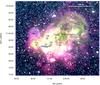 |
Fig. 1 Location of the Of-type stars in the N 206 H ii region. Three color composite image (Hα (red) + [O iii] (green) + [S ii] (blue)) shown in the background is from the Magellanic Cloud Emission-Line Survey (MCELS; Smith et al. 2005). The Of stars studied here are marked with the N206-FS number corresponding to Table 1. The dotted circle (blue) shows the rough locus of young cluster NGC 2018. The superbubble is located north-west and the SNR is at north-east of NGC 2018. |
Spectral classification
The spectral classification of the stars is primarily based on the spectral lines in the range 3960–5071 Å. We mainly followed the classification schemes proposed in Sota et al. (2011, 2014) and Walborn et al. (2014).
The main criterion for spectral classification is the He i/He ii ionization equilibrium. The diagnostic lines used for this purpose are He i lines at 4471 Å, 4713 Å, and 4387 Å compared to the He ii lines at 4200 Å and 4541 Å. However, this criterion leaves uncertainties in the subtype of the earliest O stars because of their weak or negligible He i lines.
Moreover, the strength and morphology of the optical nitrogen lines N iii λλ4634–4640–4642 (hereafter N iii), N iv λ4058 (hereafter N iv) and N v λλ4604–4620 (hereafter N v) are the fundamental classification criteria of the different Of spectral subtypes (Walborn 1971). As suggested by Walborn et al. (2002), we used the N iv λ4058/N iii λ4640 (here after N iv/N iii) and N iv λ4058/N v λ4620 (hereafter N iv/N v) emission line ratio as the primary criterion for the Of subtypes, instead of He i/He ii. The luminosity-class criteria of early O stars are mainly based on the strength of He ii 4686 and N iii lines.
The spectral type and coordinates of the nine Of-type stars are given in Table 1, together with their most prominent aliases. The corresponding normalized spectra are shown in Fig. 3. In the following, we comment on the individual Of stars.
Our sample contains one star of very early spectral subtype O2 (N206-FS 180), which was classified as an O5 V by Kavanagh et al. (2012). It is located in the bright cluster NGC 2018. The characteristic features of the O2 class in the blue spectra are strong N v absorption lines and the N iv emission significantly stronger than the N iii emission. This subtype was introduced by Walborn et al. (2002), also discussed in Rivero González et al. (2012a) and Walborn et al. (2014). The presence of strong He ii 4686 absorption shows that N206-FS 180 is a young main sequence star. According to the definition by Walborn et al. (2002), the primary characteristic of the spectral type O2 V((f*)) in comparison to O3 V((f*)) is weak or absent N iii emission. The spectrum of N206-FS 180 clearly complies with this. The presence of He i absorption lines in this very early O2 spectrum indicates a secondary component (see Sect. 3.2.2).
Two Of-type supergiants are present in the sample, N206-FS 187 and 214. N206-FS 187 was identified as binary/multiple system (Of + emission line star) in Hutchings (1980). Hutchings (1982) denoted this object as an emission line star. Kavanagh et al. (2012) classified this star as an O4-5 giant. We reclassified this spectrum as O4 If (see Table 3 and Sect. 3.1.3 of Sota et al. 2011 for more details of this classification scheme). This star is situated in the crowded region of the young cluster NGC 2018. We took the spectrum of N206-FS 186 (O8.5 (V)e), that is ≈2.5′′ away from N206-FS 187. This emission line (late Oe type) star could have been wrongly identified as a companion in previous papers (see their Hα lines in Fig. 2). Given the spacial proximity of the two stars, they were erroneously considered as a single source in several past studies.
In both supergiants N206-FS 187 and 214, the N iv emission is much weaker than the N iii emission, and the N v absorption is negligible, which indicates an O4 spectral type. Also, the He i absorption lines are almost absent or negligible in the spectra. The significant He ii 4686 emission confirms its supergiant nature. In addition to this, narrow Si iv λ4089–4116 emission features are also present in both spectra.
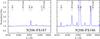 |
Fig. 2 Comparison of Hα lines of N206-FS 187 (O4 If) and neighboring star N206-FS 186 (O8.5 (V)e). |
Compared to this, N206-FS 131 has no or very weak He ii 4686 absorption and is therefore classified as bright giant (luminosity class II). The spectrum of this star shows a strong N iii emission line, but with no N v and Si iv emission lines, implying this star is cooler than previous stars (O6.5). This star is also suspected as a binary from the strength of the He i lines. Another giant with strong N iii emission is N206-FS 178 but with comparatively strong He ii 4686 absorption (luminosity class III).
Spectral type and coordinates of the nine Of-type stars in the N 206 superbubble.
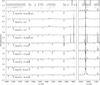 |
Fig. 3 Normalized spectra of the nine Of-type stars. The left panel depicts the medium resolution spectra in the blue (setting: LR02 and LR03). The high resolution spectra in the red (setting: HR15N) are shown in the right panelwhich includes Hα line. The central emission in Hα and the [O iii], [N ii], and [S ii] lines are from nebular emission (neb). |
We discovered two stars that exhibit special characteristics typical for the Vz class, namely, N206-FS 193 and N206-FS 111. According to Walborn (2006), these objects may be near or on the zero-age main sequence (ZAMS). As described in Walborn et al. (2014), the main characteristic of the Vz class is the prominent He ii 4686 absorption feature that is stronger than any other He line in the blue-violet region. Strong absorption in He ii 4686 corresponds to lower luminosity and a very young age (i.e., the inverse Of effect). These spectral features can be easily contaminated with strong nebular contribution, however.
Another interesting spectrum in the sample belongs to an Oef star, N206-FS 162. The Hα line is in broad emission while other Balmer lines are partially filled with disk emission, which is a feature of a classical Oe/Be star. A very small N iii emission indicates the “Of nature”. The star N206-FS 66 is classified as a subgiant. It shows weak N iii emission lines and a significant He ii 4686 absorption line.
3. The analysis
Our immediate objective is to determine the physical parameters of the individual stars. In order to analyze the FLAMES spectra, we calculated synthetic spectra using the PoWR model atmosphere code, and then fitted those to the observed spectra.
3.1. The models
The PoWR code solves the radiative transfer equation for a spherically expanding atmosphere and the statistical equilibrium equations simultaneously, while accounting for energy conservation and allowing for deviations from local thermodynamic equilibrium (i.e., non-LTE). Stellar parameters were determined iteratively. Since the hydrostatic and wind regimes of the atmosphere are solved consistently in the PoWR model (Sander et al. 2015), this code can be used for the spectroscopic analysis of any type of hot stars with winds, across a broad range of metallicities (Hainich et al. 2014, 2015; Oskinova et al. 2011; Shenar et al. 2015). More details of the PoWR code are described in Gräfener et al. (2002) and Hamann & Gräfener (2004).
A PoWR model is specified by its luminosity L, the stellar temperature T∗, the surface gravity g∗, and the mass-loss rate Ṁ as main parameters. PoWR defines the “stellar temperature” T∗ as the effective temperature referring to the stellar radius R∗ where, again by definition, the Rosseland optical depth reaches 20. In the standard definition, the “effective temperature” Teff refers to the radius R2/3 where the Rosseland optical depth is 2/3,  (1)In the case of our program stars, the winds are optically thin and the differences between T∗ and Teff are negligible. Since model spectra are most sensitive to T∗, log g∗, Ṁ, and L these parameters are varied to find the best-fit model systematically.
In the non-LTE iteration, the line opacity and emissivity profiles are Gaussian with a constant Doppler width νDop. This parameter is set to 30 km s-1 for our “Of” sample. For the energy spectra, the Doppler velocity is split into the depth-dependent thermal velocity and a “microturbulence velocity” ξ(r). We adopt ξ(r) = max(ξmin, 0.1ν(r)) for O-star models, where ξmin = 20 km s-1 (Shenar et al. 2016).
Optically thin inhomogeneities in the model iterations are prescribed by the “clumping factor” D by which the density in the clumps is enhanced compared to a homogeneous wind of the same Ṁ (Hamann & Koesterke 1998). In the current study, we account for depth-dependent clumping assuming that the clumping starts at the sonic point, increases outward, and reaches a density contrast of D = 10 at a radius of RD = 10 R∗. Note that the empirical mass-loss rates when derived from Hα emission scale with D− 1/2, since this line is mainly fed via recombination. We also varied the values of D and RD, when necessary. Higher D values and lower RD values lead to a decrease in the mass-loss rates derived from Hα.
The detailed form of the velocity field in the wind domain can affect spectral features originating in the wind. In the subsonic region, the velocity field is defined such that a hydrostatic density stratification is approached (Sander et al. 2015). In the supersonic region, the pre-specified wind velocity field ν(r) is assumed to follow the so-called β -law (Castor et al. 1975) 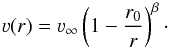 (2)In this work, we adopt β = 0.8, which is a typical value for O-type stars (Kudritzki et al. 1989).
The models are calculated using complex model atoms for H, He, C, N, O, Si, Mg, S, and P. The iron group elements (e.g., Fe, Ni) are treated with the so-called “superlevel approach” as described in Gräfener et al. (2002).
3.2. Spectral fitting
The spectral analysis is based on systematic fitting of observed spectra with grids of stellar atmosphere models. We constructed OB-star grids for LMC metallicity with the stellar temperature T∗ and the surface gravity log g∗ as parameters varied in the grid. Additional parameters such as stellar mass M and luminosity L in the grid models are chosen according to the evolutionary tracks calculated by Brott et al. (2011). The other parameters, namely the chemical composition and terminal wind velocity, are kept constant within one model grid. We also calculated some models with adjusted C, N, O, and Si abundance, when necessary. The LMC OB star grid4 spans from T∗ = 13 kK to 54 kK with a spacing of 1 kK, and log g∗ = 2.2 to 4.4 with a spacing of 0.2 dex.
We proceeded as follows to derive the stellar and wind parameters. The main method to identify the stellar temperature is to fit the He i/He ii line ratio. For the present Of-type sample we also made use of N iii/N iv/N v line ratios. The uncertainty in temperature determination according to the grid resolution is ±1 kK. Since for hotter stars, the temperature determination mainly depends on the nitrogen ionization equilibrium, and the He i lines are very weak, the uncertainty becomes larger (±2–3 kK). The surface gravity log g∗ was mainly determined from the wings of the Balmer lines, which are broadened by the Stark effect. Since the Hα line is often affected by wind emission, we mainly used Hγ and Hδ for this purpose. The typical uncertainty for log g∗ is ±0.2 dex. The uncertainty in log g∗ also propagates to the temperature and gives a total uncertainty of ~±2 kK.
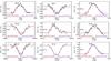 |
Fig. 4 Rotation velocity (ν sin i) from the line profile fitting of Of-type stars using the iacob-broad tool. The gray curves show the observed line profile. The ν sin i is calculated from line profile fitting based on Fourier transform method (red dotted line) and goodness-of-fit analysis (violet dashed line). See text for more details. |
We calculated two model grids; one with a mass-loss rate of 10-7M⊙ yr-1 and another with 10-8M⊙ yr-1. The mass-loss rate is scaled proportional to L3/4 to preserve the emission of recombination lines such as Hα and He ii 4686. In order to best fit the UV P-Cygni profiles and Hα line, we also calculated models with different mass-loss rates for individual stars when necessary. The primary diagnostic lines used for the mass-loss rate determination in the UV are the resonance doublets N v λλ1238–1242 and C iv λλ1548–1551 (HST/IUE range). To reproduce the N v λλ1238–1242 lines, we accounted for shock generated X-ray emission in the model. For objects that were observed by FUSE, we made use of P v λλ1118–1128, C iv at 1169 Å, and C iii at 1176 Å. For stars with available UV spectra (N206-FS 180, 187 and 214), the error in log Ṁ is approximately 0.1 dex. For the remaining stars, we derived the mass-loss rates solely on the basis of Hα and He ii 4686. If Hα is in strong absorption (no wind contamination), the mass-loss rates are based on nitrogen emission (N iii and N iv) lines with a large uncertainty. The UV P-Cygni profiles P v λλ1118–1128, N iv λ1718, and O v λ1371 provide diagnostics for stellar wind clumping in early-type O stars (Bouret et al. 2003; Martins 2011; Šurlan et al. 2013). We constrained the values of clumping parameters D and RD (also clumping onset) by consistently fitting these lines in comparison to optical lines.
The terminal velocity ν∞ defines the absorption trough of P-Cygni profiles in the UV. In contrast to the optical, UV P Cygni lines are rather insensitive to temperature and abundance variations if saturated (Crowther et al. 2002). For stars with UV spectra, we inferred the terminal velocities from these P-Cygni profiles and recalculated the models accordingly. The main diagnostic lines used are P-Cygni N v λλ1238–1242 and C iv λλ1548–1551, P v λλ1118–1128, and S v λλ1122–1134 profiles. The terminal velocity has been measured from the blue edge of the absorption component. The typical uncertainty for ν∞ is ±100 km s-1. We calculated the terminal velocities theoretically from the escape velocity νesc for those stars for which we only have optical spectra. For Galactic stars, the ratio of the terminal and escape velocity has been obtained from both theory and observations. For stars with T∗ ≥ 27 kK, the ratio is ν∞/νesc ≃ 2.6, and for stars with T∗< 27 kK the ratio is ≈1.3 (Lamers et al. 1995; Vink et al. 2001). The terminal velocity also depends on metallicity, ν∞ ∝ (Z/Z⊙)q, where q = 0.13 (Leitherer et al. 1992). We used this scaling to account for the LMC metallicity.
We calculated our models with typical LMC abundances (Trundle et al. 2007). The mass fractions of C, N, and O are varied for individual objects when necessary to best fit their observed spectra. The abundances of these elements were determined from the overall strengths of their lines with uncertainties of ~20–50%. The carbon and oxygen abundance were primarily based on C iii and O ii absorption lines. For the determination of nitrogen abundance, we particularly used the N iii absorption lines at λ4510–4525 and N v absorption lines.
Main diagnostics used in our spectral fitting process.
Finally, the projected rotation velocity ν sini is constrained from the line profile shapes. We used the iacob-broad tool implemented in IDL, which was developed by Simón-Díaz & Herrero (2014). This tool provides ν sin i values based on a combined Fourier transform (FT) and goodness-of-fit (GOF) analysis. We used two of the methods described in Simón-Díaz & Herrero (2014). In the first method, the ν sini comes from the first zero of the FT method. In this case the assumption is that macroturbulence is negligible, i.e., the additional broadening is by rotation.
The second fitting method is a combination of FT and GOF analysis, where the line profile is additionally convolved with a macroturbulent profile. The macroturbulent velocity (νmac) is calculated from the GOF when ν sini is fixed to the value corresponding to the first zero of the FT.
We selected He i, Si iv absorption lines and N iii and N iv emission lines for determining ν sini using these methods. In some cases, absorption lines which are not pressure broadened (e.g., He i and metal lines) are very weak or completely absent in the spectra. In this case, we used the iacob-broad tool on emission lines that form close to the photosphere, such as N iv 4058 and N iii 4510–4525. To ensure that the inferred values of ν sini from these emission lines are reliable, we calculated the synthetic spectrum via a 3D integration algorithm that accounts for rotation and that is appropriate for nonphotospheric lines (Shenar et al. 2014). These calculations resulted in spectra which are similar to the convolved ones. Hence, the iacob-broad tool is valid for these emission lines. For binaries, we selected those lines which have only contribution from either a primary or secondary. The fitted line profiles for individual stars are given in Fig. 4. The formal uncertainty in ν sini is ~3–8 km s-1. Corresponding to these velocities, the model spectra are convolved with rotational and macroturbulent profiles. This yields consistent fits with the observations.
The main diagnostic lines for stellar and wind parameters used in our spectral fitting process are summarized in Table 2.
The luminosity and the color excess EB−V of individual objects were determined by fitting the model SED to the photometry. The model flux is scaled with the LMC distance modulus of 18.5 mag, which corresponds to a distance of 50 kpc (Pietrzyński et al. 2013). The uncertainty in the luminosity determination is an error propagation from color excess (relatively small for LMC stars), temperature, and observed photometry. All these uncertainties give a final accuracy of about 0.2 in log L/L⊙. For stars with available flux-calibrated UV spectra (HST, IUE, or FUSE), the model SED is iteratively fitted to this calibrated spectra and normalized consistently by dividing the reddened model continuum. The uncertainty in luminosity is smaller in these cases (≈0.1 dex).
Subsequently, individual models with refined stellar parameters and abundances are calculated for each Of-type star in our sample. All these fitting processes were performed iteratively until no further improvement of the fit was possible.
3.2.1. Single star model
As an example, the fit for N206-FS 187 is given in Fig. 5. The upper panel of the figure shows the theoretical SED fitted to multiband photometry and calibrated UV spectra. We appropriately varied the reddening and luminosity for fitting the observed data with the model SED. Reddening includes the contribution from the Galactic foreground (EB−V = 0.04 mag) adopting the reddening law from Seaton (1979), and from the LMC using the reddening law described in Howarth (1983) with RV = 3.2. The total EB−V is a fitting parameter. Since flux calibrated HST/STIS and IUE spectra are available for this star, reddening and luminosity are well constrained.
The second panel shows the normalized high resolution HST/STIS UV spectrum fitted to the model. This spectrum was consistently normalized with the reddened model continuum. The last three panels show the normalized VLT-FLAMES spectrum (normalized by eye) in comparison to the PoWR spectrum.
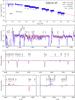 |
Fig. 5 Spectral fit for N206-FS 187. The upper panel shows the model SED (red) fitted to the available photometry from optical (UBV and I) and infrared (JHKs and IRAC 3.6 and 4.5 μm) bands (blue boxes) as well as the calibrated UV spectra from HST and IUE. The lower panels show the normalized HST and VLT-FLAMES spectra (blue solid line), overplotted with the PoWR model (red dashed line). The parameters of this best-fit model are given in Table 3. The observed spectrum also contains nebular emission lines (neb) and interstellar absorption lines (is). |
This star is best fitted with a model of T∗ = 38 kK, based on the N iii/N iv line ratio. The Balmer absorption lines in the observation are weaker compared to the model, because they are partially filled with nebular emission. The broad emission in Hα and He ii 4686 is formed in the stellar wind, which provides a constraint to the mass-loss rate.
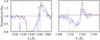 |
Fig. 6 Models with different clumping parameters are compared to the P-Cygni profiles C iv λλ1548–1551 and N iv λ1718 of N206-FS 187 (blue solid line). Dashed lines (red) are for the model with Ṁ = 2.6 × 10⁻⁶M⊙ yr-1, D = 20, and RD = 0.05 R∗. The dotted lines (black) show the model with Ṁ = 1 × 10⁻⁵M⊙ yr-1, D = 10, and RD = 10 R∗. |
The wind parameters of this star are better estimated by fitting the strong P-Cygni N v and C iv profiles. The N v λλ1238–1242 line is better reproduced by incorporating the X-ray field in the model, with X-ray luminosity LX = 4.7 × 1033 erg s-1. The X-ray field influences the ionization structure and especially strengthen this N v line (Cassinelli & Olson 1979; Baum et al. 1992). Moreover, this star is detected as a X-ray point source in XMM-Newton observation of Kavanagh et al. (2012). Its strong X-ray luminosity might be due to binarity (see Sect. 4.3), but we do not see any sign of secondary component in the spectra. Therefore, the star is here fitted as a single star.
The left panel of Fig. 6 shows the C iv λλ1548–1551 resonance doublet. We measured ν∞ from its blue edge as 2300 ± 50 km s-1. Since this line is saturated, it is not sensitive to clumping. But the N iv λ1718 line shown in the right panel is unsaturated, and found to be weaker in the observed spectrum than in the model. This could be an indication of strongly clumped wind. Figure 6 compares two models with different clumping parameters as described in Sect. 3.1. In order to decrease the strength of the N iv λ1718 P-Cygni profile in the model, clumping should start before the sonic point and reach its maximum value D already at a very low radius. The model with a density contrast D = 20 and the clumping starts at a radius of 0.025R∗ and reaches the maximum value of D at RD = 0.05 R∗, best reproduces the observation (see right panel of Fig. 6). Since clumping enhances the emission of Hα, we decreased the mass-loss rate by a factor of 4 compared to the model with the default clumping. The O v λ1371 line is similarly affected by wind clumping. However, the strong X-ray luminosity and possible binarity (see Sect. 4.3) of this source might be related to the strength of these lines.
3.2.2. Composite model
The spectrum of N206-FS 187 shown in Fig. 5 is satisfactorily fitted by a single-star model. However, there are two objects in our sample (N206-FS 180, N206-FS 131) for which the observed spectra cannot be reproduced by a single synthetic spectrum.
The spectrum of N206-FS 180 is shown in Fig. B.7. The weakness of the N iii lines, N iv lines in emission, and the presence of strong N v absorption lines indicate a very high stellar temperature. We selected the temperature of the model so that the synthetic spectrum reproduces the observed N iv/N v and N iii/N iv line ratios. The best fit is achieved for T∗ = 50 kK and log g∗ = 4.2. Since the temperature of this model is very high, it does not predict any He i lines to show up. Hence, the small He i absorption lines in the observed spectrum can be attributed to a companion, which must be an O star of late subtype (later than O6 to produce He i absorption lines, but earlier than B0 since Si, C, O, and Mg absorption lines are absent).
The observed spectrum is fully reproduced with a composite model (see Fig. B.8). The final model spectrum is the sum of an early-type Of star O2 V((f*)) and an O8-9 star. The light ratio of the components is constrained by the diluted strength of absorption features which are attributed to the secondary component (Shenar et al. 2016). These absorption features should be insensitive to the remaining stellar parameters. In our case of N206-FS 180, the He i lines at 4388 Å, 4472 Å, and 4922 Å are available for this purpose. Here our main assumption is that the primary component is more luminous and hotter than the secondary. We also ensured that the primary model perfectly reproduces the N v and N iv lines, assuming that they have no contribution from the secondary component (late O-type). The individual and the composite SEDs are depicted in the upper panel of Fig. B.8.
The luminosity and reddening derived from fitting IUE-short spectrum and photometric data are different. The UV spectrum fit best with a model SED of high luminosity log L/L⊙ = 6.47, while the photometry is best fitted with a SED having log L/L⊙ = 6.11 (primary). Both the high resolution and low resolution IUE spectrum (flux calibrated) show deviation from the photometry. Since the aperture of the IUE is large (≈21″ × 9″) and the star belongs to the crowded region of the cluster, the observed spectrum is likely to be contaminated from nearby stars. So, we have adapted the luminosity corresponding to photometry.
For those stars which show Hα in absorption, the mass-loss rate and terminal velocity can be solely derived from UV spectra. For N206-FS 180, the normalized IUE spectrum is shown in the second panel of Fig. B.7. The P-Cygni O v line at 1371 Å is stronger in the model than in the observation, which usually indicates strong wind clumping. But according to Massey et al. (2005) if Hα is in absorption, the only wind contribution is from layers very close to the sonic point, so absorption-type profiles are hardly affected by clumping. Apart from this, we could not fit the observed spectrum using a model with stronger clumping prescriptions. Hence, we consider only the default clumping with D = 10 in the model (see Sect. 3.1).
Since this star is still in the hydrogen burning phase, the increase in nitrogen abundance would result in a lower oxygen abundance (CNO balance). Models with three different oxygen mass fractions (varied by a factor of 10) are compared to the O v line in Fig. 7. We can only reproduce this line with a model with 100 times lower oxygen abundance compared to the typical LMC value. However, the total CNO abundance of this model is inconsistent with the typical LMC values.
The nitrogen lines of N v and N iv in the optical are also found to be affected by changing the mass-loss rate and terminal velocity in the model. We estimate Ṁ = 7 × 10⁻⁶M⊙ yr-1 for the primary from the best fit. The terminal velocity measured from the blue edge of C iv λλ1548–1551 is 2800 km s-1. In the cases where UV spectra are not available and Hα is in absorption, Ṁ has a large uncertainty and ν∞ is theoretically determined as described in Sect. 3.2.
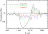 |
Fig. 7 O v P-Cygni line profile of N206-FS 180 (blue solid line). Three models with different oxygen mass fractions (see labels) are shown for comparison. |
We suspect the star N206-FS 131 also to be a binary. The remaining Of stars are well fitted with single star models. Individual descriptions and spectral fits of all stars of our sample are given in Appendix A and Appendix B, respectively.
4. Results and discussions
4.1. Stellar parameters
Stellar parameters of nine Of-type stars in N 206 superbubble.
The fundamental parameters for the individual stars are given in Table 3. The rate of hydrogen ionizing photons (log Q) and the mechanical luminosity of the stellar winds ( ) are also tabulated. All these models are calculated with default clumping parameters as described in Sect. 3.1.
The gravities shown here are not corrected for rotation. The effect is insignificant and much less than the uncertainty values, even for the fastest rotating star in our sample (log (g∗ + (ν sin i)2/R∗)−log g∗< 0.03). The reddening of our sample stars is only 0.1–0.3 mag (see Table 3). The absolute visual magnitudes (MV) in the table are also derived from the respective models. The spectroscopic masses, calculated from log g∗ and R∗ (using relation  ), are in the range 30–150 M⊙.
For the binary candidates N206-FS 180 and N206-FS 131, the stellar parameters for the individual components (“a” denotes the primary and “b” the secondary component) are given in the table as well. Only the primaries of these binary systems are considered in the following discussions.
Figure 8 shows how the effective temperature correlates with the spectral subtypes of our sample. Different luminosity classes are denoted using squares, triangles, and circles for luminosity class V-IV, III-II, and I, respectively. The O2 subtype shows an outstandingly high effective temperature, T∗ = 50 kK, which is comparable to the temperatures of other O2 stars (e.g., Rivero González et al. 2012a,b; Walborn et al. 2004). This supports the results of Mokiem et al. (2007) and Rivero González et al. (2012b,a), who suggest a steeper slope in the temperature – spectral type relation for the earliest subtypes (O2-O3).
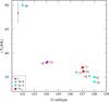 |
Fig. 8 Effective temperature as a function of spectral type. Squares, triangles, and circles denote the luminosity classes Vz, V-IV, III-II and I, respectively. Typical uncertainties are indicated by the error bar in the upper left corner. |
4.2. Wind parameters
In addition to the stellar parameters, the spectra provide information on the stellar winds of our sample. The primary stellar wind parameters are wind terminal velocities (ν∞) and mass-loss rates (Ṁ). The mass-loss rate has great influence on the evolution of massive stars. The Ṁ scales with the metallicity of stars (Leitherer et al. 1992; Vink et al. 2001). The lower LMC metallicity results in less efficient wind driving in comparison to the Galactic environment, and consequently in lower mass-loss rates (Vink et al. 2000).
For stars with available UV spectra (N206-FS 180, N206-FS 187, and N206-FS 214), the mass-loss rate is obtained from P Cygni lines as explained in Sect. 3.2. For N206-FS 131, Hα is partially filled with wind emission, and the corresponding spectral fit yields Ṁ. The rest of the sample shows Hα in pure absorption, so the Ṁ values are estimated from the nitrogen emission lines. Since these nitrogen lines are also affected by the nitrogen abundance, these mass-loss rates have an additional uncertainty. The derived mass-loss rates of our Of samples are in the range from 10-6.9 to 10-4.8M⊙ yr-1.
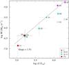 |
Fig. 9 Mass-loss rates vs. luminosity for the Of stars in the N 206 superbubble in the LMC. Open circles denote alternative values for the two supergiants obtained with stronger clumping (see Sect. 3.2.1). A power law is fitted to the data points. Symbols have the same meaning as in Fig. 8. The error bars are shown for each source. |
Mass-loss rate and luminosity exhibit a clear correlation in Fig. 9. Here the supergiants are in the upper right corner with high luminosity and Ṁ. This relation can be fitted as a power-law with an exponent ≈1.5 (uncertainties are considered in the fit). The models of two supergiants with alternative clumping prescriptions (see Sect. 3.2.1) would yield a lower mass-loss rate by a factor 5 (open circles). The supergiant N206-FS 187 has a very high luminosity and mass-loss rate, even compared to the Galactic stars with the same spectral type. A star (VFTS 1021) with similar high values of L and Ṁ has been found by Bestenlehner et al. (2014).
Wind-momentum luminosity relationship
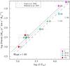 |
Fig. 10 Modified wind momentum (Dmom) in units of M⊙ yr-1 km s |

To investigate the winds of Of stars in the LMC quantitatively, we plotted the modified wind momentum – luminosity relation (WLR) in Fig. 10. This diagram depicts the modified stellar wind momentum  (Kudritzki & Puls 2000), as a function of the stellar luminosity.
For the WLR, a relation in the form  (3)is expected, where x corresponds to the inverse of the slope of the line-strength distribution function, and D0 is related to the effective number of lines contributing to stellar wind acceleration (Puls et al. 2000). The distribution of line strengths is important to compare the observed wind strengths to the predictions of line driven wind theory. A linear regression to the logarithmic values of the modified wind momenta obtained in this work (see Fig. 10) yields the relation
  (4)Figure 10 also shows the relation for the LMC stars (x = 1.83) as predicted by Vink et al. (2000). The dotted lines represent the empirical WLR for LMC OB stars (x = 1.81) as determined by Mokiem et al. (2007). Bestenlehner et al. (2014) also found an empirical WLR for O stars in the 30 Doradus region of the LMC with x = 1.45. The Of stars in the superbubble N 206 shows a good correlation with both empirical and theoretical WLR. It should be noted that for the wind momentum calculation of some of the sources, we adopted theoretical ν∞ values in the absence of available the UV spectrum. The uncertainties of parameters are also estimated and included in the linear regression.
The wind momenta of the supergiants would be much lower if strong clumping is adopted (open circles). Figure 10 shows the WLR with default clumping as described in Sect. 3.2.1 for all the stars. This is close to the theoretical relation (x ~ 1.8). The alternative clumping prescriptions for two supergiants (strong clumping) would result a less steeper WLR relation. Mokiem et al. (2007) also tested clumping corrections for one supergiant and obtained a less steep relation (x ~ 1.43). Note that the theoretical WLR is based on unclumped winds. In our analysis, a depth dependent clumping was accounted for all stars.
4.3. Outstanding X-ray luminosity of N206-FS 187 points to its binarity
The supergiant N206-FS 187 was detected in X-rays with the XMM-Newton telescope (Kavanagh et al. 2012). Since no X-ray spectral information was presented by Kavanagh et al. (2012), we adopted the X-ray flux from “The third XMM-Newton serendipitous source catalog” (Rosen et al. 2016). Correcting for interstellar absorption, NH = 9 × 1021 cm-2 (Kavanagh et al. 2012), the estimated X-ray luminosity of N206-FS 187 is LX ≈ 4 × 1034 erg s-1 in the 0.2–12.0 keV band. Hence, the ratio between X-ray and bolometric luminosity is log LX/Lbol ≈ −5.
This is an outstandingly high X-ray luminosity for an O-type star. Single O-type stars in the Galaxy have significantly lower X-ray luminosities (e.g., Oskinova 2005). The high X-ray luminosity of N206-FS 187 might indicate that this object is a binary. In a massive binary, the bulk of X-ray emission might be produced either by collision of stellar winds from binary components, or by accretion of stellar wind if the companion is a compact object.
Some colliding wind binaries consisting of a WR and an O-type component have comparably high X-ray luminosities (Portegies Zwart et al. 2002; Guerrero & Chu 2008). However our spectral analysis of N206-FS 187 rules out a WR component. Most likely, the binary component in N206-FS 187 is an O-type star of similar spectral type. Even in this case, it is outstandingly X-ray luminous. For example, the X-ray luminosity of the O3.5If* + O3.5If* binary LS III+46 11 is an order of magnitude lower than that of N206-FS 187 (Maíz Apellániz et al. 2015, and references therein). Some wind-wind colliding (WWC) feature may be present in the lines such as Hα (Moffat 1989). However, as the WWC effects are usually of the order of a few percentage (Hill et al. 2000), that are not expected to highly influence the spectral features.
On the other hand, the X-ray luminosity of N206-FS 187 is not in the correct range to suspect that it harbors a compact companion. The latter systems are either usually significantly more X-ray luminous (in case of persistent sources), or significantly less X-ray luminous in quiescence (in case of transients) (Martínez-Núñez et al. 2017).
Therefore, on the basis of the high X-ray luminosity of N206-FS 187 and taking into account the uncertainties on its X-ray spectral properties, we believe that N206-FS 187 is one of the X-ray brightest colliding wind binaries consisting of stars with similar spectral types. Interestingly the other Of supergiant N206-FS 214 does not show any X-ray emission, even though it is an eclipsing binary of similar spectral types (see Appendix A for more details).
Note that the X-ray luminosity derived from our model using UV spectral line fit (LX ≈ 4.7 × 1033 erg s-1) is an order of magnitude less than this observed X-ray luminosity (see Sect. 3.2.1). One reason could be the variability of X-ray emission if it is a WWC binary. Another possibility is that the observed X-ray luminosity might be overestimated from the interstellar absorption values.
4.4. The Hertzsprung-Russell diagram
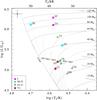 |
Fig. 11 Hertzsprung-Russell diagram for the nine Of stars in the N 206 superbubble in the LMC. The evolutionary tracks and isochrones are based on rotating (Vrot,init ~ 100 km s-1) evolutionary models presented in Brott et al. (2011) and Köhler et al. (2015). Different luminosity classes are denoted using rhombus, squares, triangles, and circles for luminosity class Vz, V-IV, III-II, and I, respectively. The position of the secondary components of N206-FS 131 and N206-FS 180 are also marked in the diagram with a cross symbol. |
The Hertzsprung-Russell diagram (HRD) for the Of stars in the N 206 superbubble, constructed from the temperature and luminosity estimates (see Table 3), is given in Fig. 11. The evolutionary tracks and isochrones are adapted from Brott et al. (2011) and Köhler et al. (2015), accounting for an initial rotational velocity of ~100 km s-1. The evolutionary tracks are shown for stars with initial masses of 15–125 M⊙, while the isochrones span from the zero age main sequence (ZAMS) to 5 Myr in 1 Myr intervals. Stars are represented by respective luminosity class symbols as in Fig. 11.
The isochrones suggest that the O2((f*)) star N206-FS 180 (primary) is very young and close to the ZAMS (assuming single-star evolution). The evolutionary mass predicted from the tracks is ≈93 M⊙ for the primary component of this binary system. The other Of stars are younger than ≈4 Myr and more massive than ≈25 M⊙. The supergiants in our sample are nearly 2 Myr old with masses in the range 70 to 100 M⊙.
The evolutionary masses from the HRD are compared in Fig. 12 to the spectroscopic masses derived (see Table 3). Here, the evolutionary mass refers to the current stellar mass as predicted by the corresponding evolutionary track. It is evident from Fig. 12 that the spectroscopic masses of the objects are systematically larger than their evolutionary masses. However we have to acknowledge that, the errors in our spectroscopic mass estimates are large (at least a factor 2). The wind contamination in the Balmer wings also affects the log g determination, and we adopt theoretical values for ν∞ in some cases.
This mass discrepancy problem was extensively investigated for Galactic and extragalactic star clusters by many authors (Herrero et al. 1992; Vacca et al. 1996; Repolust et al. 2004). This mass difference is strongly affected by the mass-loss recipe used in the evolutionary calculations (McEvoy et al. 2015). According to Hunter et al. (2008), the observed mass discrepancy of main-sequence stars could be due to binarity, errors in the distance estimate, bolometric corrections, reddening, or the derived surface gravities. However, the systematic trend in the discrepancy may not be due to the uncertainties in our parameter measurements, but could originate from the evolutionary masses.
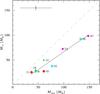 |
Fig. 12 Evolutionary masses compared to the spectroscopic masses. The discrepancy grows roughly linearly with the mass (see linear fit). The one-to-one correlation of spectroscopic and evolutionary masses is indicated by the dashed line. |
4.5. Chemical abundance
Chemical abundance for the nine Of-type stars in the N 206 superbubble derived from spectral fitting.
The chemical abundances of our Of sample derived in terms of mass fraction are given in Table 4. These have been obtained by fitting the observed spectra with PoWR models calculated for different C, N, and O mass fractions (see Table 2 for more details). Since the nitrogen lines are formed by complex NLTE processes, changes in the N abundance can have a large impact on the strength of the lines (Rivero González et al. 2012b). The P, Mg, Si, and S abundances are fixed for all the models. We could not reproduce the Si iv emission lines in supergiants N206-FS 187 and N206-FS 214 with our models.
The distribution of nitrogen abundances with effective temperature is illustrated in Fig. 13. We can see a direct correlation in our sample (except N206-FS 111). In addition, all these stars show lower abundance in either oxygen or carbon (compared to typical LMC values) due to the CNO process. The O2 spectral type shows a very high nitrogen abundance in comparison to the other Of stars (but less than the total CNO mass fraction). In turn, its oxygen abundance measured from the O v line at 1371 Å is much lower by a factor of 100 than the typical LMC values.
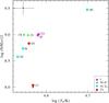 |
Fig. 13 Surface nitrogen abundances as a function of the effective temperature. The downward arrow indicates an upper limit to the nitrogen abundance of N206-FS 111. |
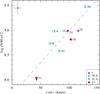 |
Fig. 14 Surface nitrogen abundances as a function of the projected rotation velocity ν sin i. The dashed line is a linear regression to the data. The downward arrow indicates an upper limit to the nitrogen abundance of N206-FS 111. |
One of the key questions of massive star evolution is rotational mixing and its impact on the nitrogen abundance. Evolutionary models accounting for rotation (Hunter et al. 2008; Brott et al. 2011; Rivero González et al. 2012b,a) predict that the faster a star rotates, the more mixing will occur, and the larger the nitrogen surface abundance that should be observed. Figure 14 shows a so-called “Hunter-diagram”, depicting the variation of the nitrogen enrichment with the projected rotational velocity. Our Of sample shows projected rotational velocities in the range of ~40–130 km s-1 and nitrogen abundances (log (N/H) +12) from 8 to 9.6. This diagram shows a relative increase in nitrogen abundance with rotation. It should be noted that the projected rotational velocity and the true rotational velocity differ by a factor sin i. However, Maeder et al. (2009) suggests that chemical enrichment is not only a function of projected rotational velocity, but also depends on ages, masses, and metallicities. The nitrogen enriched stars are very massive in our case.
The following conclusions can be made from the diagram:
-
The O2 dwarf N206-FS 180 shows aexceptionally high nitrogen abundance, and its projectedrotational velocity is highest among the sample.
-
Evolved stars (giants and supergiants) are more nitrogen enriched than dwarfs of the same effective temperature.
-
The slowest rotator in our sample (also least massive), N206-FS 111 (ν sin i = 43 km s-1), shows very little enrichment. Although N206-FS 111 and N206-FS 193 are ZAMS candidates (Vz), N206-FS 193 (ν sin i = 103 km s-1) shows nitrogen enhancement.
-
The two binary candidates (N206-FS 180a and N206-FS 131a) are more nitrogen enriched than other stars with similar rotational velocities.
According to Kohler et al. (2015), a strong nitrogen surface enhancement can be obtained even in models with initial rotational velocities well below the threshold value. All our sample stars are nitrogen enriched with rotational velocities below 200 km s-1. Because of the strong mass loss and large convective core masses, their evolutionary models above 100 M⊙ shows nitrogen-enrichment irrespective of their rotation rate. The large nitrogen enhancement in our sample star N206-FS 180 is very similar (M ≈ 100 M⊙, νsin i ≈ 150 km s-1, age ≈ 1 Myr) to their model predictions. Moreover, this source is a part of binary system, which may also have influence in the enrichment.
4.6. Stellar feedback
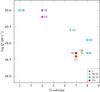 |
Fig. 15 Rate of ionizing photons as a function of the O subtype. |
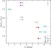 |
Fig. 16 Mechanical luminosity of stellar winds as a function of the O subtype. The open circles for the two supergiants refers to the models with alternative solution with higher clumping. Typical uncertainties are indicated with error bar in the upper right corner. |
The main contribution to the stellar feedback in the N 206 superbubble is expected to come from stars in our Of sample. The number of ionizing photons and the mechanical luminosity of the stellar winds as a function of O subtypes are shown in Figs. 15 and 16. Both of these energy feedback mechanisms show a correlation with spectral subtype, where the O2((f*)) star and the two supergiants dominate. The combined ionizing photon flux from the nine Of stars is approximately Q0 ≈ 3 × 1050 s-1. The total mechanical feedback from these Of stars is  6.5 × 1037erg s-1). We stress that the ν∞ was adopted for majority of the sample. The uncertainties in these estimates are propagated from mass-loss rate and terminal velocity. As now discussed, the total mechanical luminosity is dominated by the three Of stars, for which an uncertainty of approximately 30% is estimated. Assuming stronger clumping in models would lower this total feedback by a factor of two.
Kavanagh et al. (2012) analyzed the X-ray superbubble in N 206 using XMM-Newton data. The thermal energy stored in the superbubble was estimated using the X-ray emitting gas, the kinetic energy of the Hα shells, and the kinetic energy of the surrounding H i gas. Using spectral fits Kavanagh et al. (2012) derived the physical properties of the hot gas and hence estimated the thermal energy content of the X-ray superbubble. Along with this, they calculated the kinetic energy of the expansion of the shell in the surrounding neutral gas using MCELS and 21 cm line emission line data from the ATCA-Parkes survey of the Magellanic Clouds (Kim et al. 1998). They estimated the total energy to be (4.7 ± 1.3) × 1051 erg.
This thermal energy could be supplied by the stars in the N206 superbubble via stellar winds and the supernova occurred in this region (SNR B0532-71.0). We calculated the current mechanical energy supply from these Of stars. In order to provide the total energy estimate of these Of-type stars, we must derive their current ages. So, we adopted the ages of individual stars from the HRD (see Sect. 4.4) using isochrone fitting. The total mechanical energy supplied by these stars throughout their lifetimes is (5.8 ± 1.8) × 1051 erg. As in Kavanagh et al. (2012), we also assumed that these stars provide same amount of mechanical energy throughout their lifetime, since they are very young. Also, the time duration is short for a significant contribution from radiative and other cooling processes, and can be neglected for this rough estimate. The energy estimates are consistent with Kavanagh et al. (2012), even though we consider only the mechanical feedback from stellar winds. The total momentum provided from these stars over time is ≈1.86 × 1043 g cm s-1.
This shows that the Of stars in our sample provide a significant contribution to the energy feedback. The total feedback in the superbubble including the entire OB population, Wolf-Rayet stars (BAT99 53, BAT99 49), and supernova will be discussed in Paper II.
5. Summary and conclusions
We have obtained and analyzed FLAMES spectra of nine massive Of-type stars in the N 206 giant H ii complex located in the LMC. On the basis of these data complemented by archival UV spectra, we determined precise spectral types and performed a thorough spectral analysis. We used sophisticated PoWR model atmospheres to derive the physical and wind parameters of the individual stars. Our main conclusions are as follows.
-
All stars have an age less than 4 Myr. The earliest O2 star appears to be less than 1 Myr old, while the two supergiants are 2 Myr old.
-
The wind-momentum luminosity relation of our sample are comparable to that of theoretically predicted, with the assumption of a depth dependent clumping in all models.
-
The star N206-FS 187 shows very high mass-loss rate and luminosity. Its large X-ray luminosity suggests that this object is one of the X-ray brightest colliding wind binaries consisting of stars with similar spectral types.
-
Most of the Of stars are nitrogen enriched. A clear trend toward more enrichment with rotation as well as with temperature is found. The binary stars and more evolved stars show nitrogen enrichment compared to others.
-
The O2 star N206-FS 180 shows a very high nitrogen mass fraction, while oxygen is strongly depleted compared to the typical LMC values.
-
The evolutionary masses are systematically lower than the corresponding spectroscopic masses obtained from our analysis.
-
The total ionizing photon flux and stellar wind mechanical luminosity of the Of stars are estimated to 3 × 1050 s-1 and 1.7 × 10⁴L⊙, respectively. This leads us to conclude that the program stars play a significant role in the evolution of the N 206 superbubble.
The subsequent paper (Ramachandran et al., in prep.) will provide the detailed analysis and discussion of complete OB star population in the N 206 superbubble.
VLT-PRO-ESO-19000-1930/1.0/27-Sep-99 VLT Data Flow System, Gasgano DFS File Organizer Design Document.
Acknowledgments
V.R. is grateful for financial support from Deutscher Akademischer Austauschdienst (DAAD), as a part of Graduate School Scholarship Program. L.M.O. acknowledges support by the DLR grant 50 OR 1508. A.S. is supported by the Deutsche Forschungsgemeinschaft (DFG) under grant HA 1455/26. T.S. acknowledges support from the German “Verbundforschung” (DLR) grant 50 OR 1612. We thank C. J. Evans for helpful discussions. This research made use of the VizieR catalog access tool, CDS, Strasbourg, France. The original description of the VizieR service was published in A&AS 143, 23. Some data presented in this paper were obtained from the Mikulski Archive for Space Telescopes (MAST). STScI is operated by the Association of Universities for Research in Astronomy, Inc., under NASA contract NAS5-26555. Support for MAST for non-HST data is provided by the NASA Office of Space Science via grant NNX09AF08G and by other grants and contracts. We thank the anonymous referee for valuable comments and suggestions.
References
- Baum, E., Hamann, W.-R., Koesterke, L., & Wessolowski, U. 1992, A&A, 266, 402 [NASA ADS] [Google Scholar]
- Bestenlehner, J. M., Gräfener, G., Vink, J. S., et al. 2014, A&A, 570, A38 [NASA ADS] [CrossRef] [EDP Sciences] [Google Scholar]
- Bonanos, A. Z., Massa, D. L., Sewilo, M., et al. 2009, AJ, 138, 1003 [NASA ADS] [CrossRef] [Google Scholar]
- Bouret, J.-C., Lanz, T., Hillier, D. J., et al. 2003, ApJ, 595, 1182 [NASA ADS] [CrossRef] [Google Scholar]
- Brott, I., de Mink, S. E., Cantiello, M., et al. 2011, A&A, 530, A115 [NASA ADS] [CrossRef] [EDP Sciences] [Google Scholar]
- Cassinelli, J. P., & Olson, G. L. 1979, ApJ, 229, 304 [NASA ADS] [CrossRef] [Google Scholar]
- Castor, J. I., Abbott, D. C., & Klein, R. I. 1975, ApJ, 195, 157 [NASA ADS] [CrossRef] [Google Scholar]
- Crowther, P. A., Dessart, L., Hillier, D. J., Abbott, J. B., & Fullerton, A. W. 2002, A&A, 392, 653 [NASA ADS] [CrossRef] [EDP Sciences] [Google Scholar]
- Evans, C. J., Taylor, W. D., Hénault-Brunet, V., et al. 2011, A&A, 530, A108 [NASA ADS] [CrossRef] [EDP Sciences] [Google Scholar]
- Gorjian, V., Werner, M. W., Mould, J. R., et al. 2004, ApJS, 154, 275 [NASA ADS] [CrossRef] [Google Scholar]
- Graczyk, D., Soszyński, I., Poleski, R., et al. 2011, Acta Astron., 61, 103 [Google Scholar]
- Gräfener, G., Koesterke, L., & Hamann, W.-R. 2002, A&A, 387, 244 [NASA ADS] [CrossRef] [EDP Sciences] [Google Scholar]
- Gruendl, R. A., & Chu, Y.-H. 2009, ApJS, 184, 172 [Google Scholar]
- Guerrero, M. A., & Chu, Y.-H. 2008, ApJS, 177, 216 [NASA ADS] [CrossRef] [Google Scholar]
- Hainich, R., Rühling, U., Todt, H., et al. 2014, A&A, 565, A27 [NASA ADS] [CrossRef] [EDP Sciences] [Google Scholar]
- Hainich, R., Pasemann, D., Todt, H., et al. 2015, A&A, 581, A21 [Google Scholar]
- Hamann, W.-R., & Gräfener, G. 2004, A&A, 427, 697 [NASA ADS] [CrossRef] [EDP Sciences] [Google Scholar]
- Hamann, W.-R., & Koesterke, L. 1998, A&A, 335, 1003 [NASA ADS] [Google Scholar]
- Herrero, A., Kudritzki, R. P., Vilchez, J. M., et al. 1992, A&A, 261, 209 [NASA ADS] [Google Scholar]
- Hill, G. M., Moffat, A. F. J., St.-Louis, N., & Bartzakos, P. 2000, MNRAS, 318, 402 [NASA ADS] [CrossRef] [Google Scholar]
- Howarth, I. D. 1983, MNRAS, 203, 301 [NASA ADS] [CrossRef] [Google Scholar]
- Howarth, I. D. 2013, A&A, 555, A141 [NASA ADS] [CrossRef] [EDP Sciences] [Google Scholar]
- Hunter, I., Brott, I., Lennon, D. J., et al. 2008, ApJ, 676, L29 [NASA ADS] [CrossRef] [Google Scholar]
- Hutchings, J. B. 1980, ApJ, 235, 413 [NASA ADS] [CrossRef] [Google Scholar]
- Hutchings, J. B. 1982, ApJ, 255, 70 [NASA ADS] [CrossRef] [Google Scholar]
- Kavanagh, P. J., Sasaki, M., & Points, S. D. 2012, A&A, 547, A19 [NASA ADS] [CrossRef] [EDP Sciences] [Google Scholar]
- Kim, S., Staveley-Smith, L., Dopita, M. A., et al. 1998, ApJ, 503, 674 [NASA ADS] [CrossRef] [Google Scholar]
- Köhler, K., Langer, N., de Koter, A., et al. 2015, A&A, 573, A71 [NASA ADS] [CrossRef] [EDP Sciences] [Google Scholar]
- Kudritzki, R.-P., & Puls, J. 2000, ARA&A, 38, 613 [NASA ADS] [CrossRef] [Google Scholar]
- Kudritzki, R. P., Pauldrach, A., Puls, J., & Abbott, D. C. 1989, A&A, 219, 205 [NASA ADS] [Google Scholar]
- Lamers, H. J. G. L. M., Snow, T. P., & Lindholm, D. M. 1995, ApJ, 455, 269 [NASA ADS] [CrossRef] [Google Scholar]
- Leitherer, C., Robert, C., & Drissen, L. 1992, ApJ, 401, 596 [NASA ADS] [CrossRef] [Google Scholar]
- Lindsay, E. M. 1963, Ir. Astron. J., 6, 127 [NASA ADS] [Google Scholar]
- Mac Low, M.-M., & McCray, R. 1988, ApJ, 324, 776 [NASA ADS] [CrossRef] [Google Scholar]
- Madore, B. F., & Freedman, W. L. 1998, ApJ, 492, 110 [NASA ADS] [CrossRef] [Google Scholar]
- Maeder, A., Meynet, G., Ekström, S., & Georgy, C. 2009, Commun. Asteroseismol., 158, 72 [NASA ADS] [Google Scholar]
- MaízApellániz, J., Negueruela, I., Barbá, R. H., et al. 2015, A&A, 579, A108 [NASA ADS] [CrossRef] [EDP Sciences] [Google Scholar]
- Martínez-Núñez, S., Kretschmar, P., Bozzo, E., et al. 2017, Space Sci. Rev., 212, 59 [NASA ADS] [CrossRef] [Google Scholar]
- Martins, F. 2011, Bull. Soc. Roy. Sci. Liège, 80, 29 [Google Scholar]
- Massey, P., Lang, C. C., Degioia-Eastwood, K., & Garmany, C. D. 1995, ApJ, 438, 188 [NASA ADS] [CrossRef] [Google Scholar]
- Massey, P., Puls, J., Pauldrach, A. W. A., et al. 2005, ApJ, 627, 477 [NASA ADS] [CrossRef] [Google Scholar]
- McEvoy, C. M., Dufton, P. L., Evans, C. J., et al. 2015, A&A, 575, A70 [NASA ADS] [CrossRef] [EDP Sciences] [Google Scholar]
- Moffat, A. F. J. 1989, ApJ, 347, 373 [NASA ADS] [CrossRef] [Google Scholar]
- Mokiem, M. R., de Koter, A., Evans, C. J., et al. 2007, A&A, 465, 1003 [NASA ADS] [CrossRef] [EDP Sciences] [Google Scholar]
- Oskinova, L. M. 2005, MNRAS, 361, 679 [NASA ADS] [CrossRef] [Google Scholar]
- Oskinova, L. M., Todt, H., Ignace, R., et al. 2011, MNRAS, 416, 1456 [NASA ADS] [CrossRef] [Google Scholar]
- Pasquini, L., Avila, G., Blecha, A., et al. 2002, The Messenger, 110, 1 [NASA ADS] [Google Scholar]
- Pietrzyński, G., Graczyk, D., Gieren, W., et al. 2013, Nature, 495, 76 [NASA ADS] [CrossRef] [PubMed] [Google Scholar]
- Portegies Zwart, S. F., Pooley, D., & Lewin, W. H. G. 2002, ApJ, 574, 762 [NASA ADS] [CrossRef] [Google Scholar]
- Puls, J., Springmann, U., & Lennon, M. 2000, A&AS, 141, 23 [NASA ADS] [CrossRef] [EDP Sciences] [Google Scholar]
- Ramírez-Agudelo, O. H., Sana, H., de Koter, A., et al. 2017, A&A, 600, A81 [NASA ADS] [CrossRef] [EDP Sciences] [Google Scholar]
- Repolust, T., Puls, J., & Herrero, A. 2004, A&A, 415, 349 [NASA ADS] [CrossRef] [EDP Sciences] [Google Scholar]
- Rivero González, J. G., Puls, J., Massey, P., & Najarro, F. 2012a, A&A, 543, A95 [NASA ADS] [CrossRef] [EDP Sciences] [Google Scholar]
- Rivero González, J. G., Puls, J., Najarro, F., & Brott, I. 2012b, A&A, 537, A79 [NASA ADS] [CrossRef] [EDP Sciences] [Google Scholar]
- Rolleston, W. R. J., Trundle, C., & Dufton, P. L. 2002, A&A, 396, 53 [NASA ADS] [CrossRef] [EDP Sciences] [Google Scholar]
- Romita, K. A., Carlson, L. R., Meixner, M., et al. 2010, ApJ, 721, 357 [NASA ADS] [CrossRef] [Google Scholar]
- Rosen, S. R., Webb, N. A., Watson, M. G., et al. 2016, A&A, 590, A1 [NASA ADS] [CrossRef] [EDP Sciences] [Google Scholar]
- Sander, A., Shenar, T., Hainich, R., et al. 2015, A&A, 577, A13 [NASA ADS] [CrossRef] [EDP Sciences] [Google Scholar]
- Seaton, M. J. 1979, MNRAS, 187, 73P [NASA ADS] [CrossRef] [Google Scholar]
- Shenar, T., Hamann, W.-R., & Todt, H. 2014, A&A, 562, A118 [NASA ADS] [CrossRef] [EDP Sciences] [Google Scholar]
- Shenar, T., Oskinova, L., Hamann, W.-R., et al. 2015, ApJ, 809, 135 [NASA ADS] [CrossRef] [Google Scholar]
- Shenar, T., Hainich, R., Todt, H., et al. 2016, A&A, 591, A22 [NASA ADS] [CrossRef] [EDP Sciences] [Google Scholar]
- Simón-Díaz, S., & Herrero, A. 2014, A&A, 562, A135 [NASA ADS] [CrossRef] [EDP Sciences] [Google Scholar]
- Smith, R. C., Points, S., Chu, Y.-H., et al. 2005, in American Astronomical Society Meeting Abstracts, BAAS, 37, 145.01 [Google Scholar]
- Sota, A., Maíz Apellániz, J., Walborn, N. R., et al. 2011, ApJS, 193, 24 [NASA ADS] [CrossRef] [Google Scholar]
- Sota, A., Maíz Apellániz, J., Morrell, N. I., et al. 2014, ApJS, 211, 10 [NASA ADS] [CrossRef] [Google Scholar]
- Šurlan, B., Hamann, W.-R., Aret, A., et al. 2013, A&A, 559, A130 [NASA ADS] [CrossRef] [EDP Sciences] [Google Scholar]
- Trundle, C., Dufton, P. L., Hunter, I., et al. 2007, A&A, 471, 625 [NASA ADS] [CrossRef] [EDP Sciences] [Google Scholar]
- Vacca, W. D., Garmany, C. D., & Shull, J. M. 1996, ApJ, 460, 914 [NASA ADS] [CrossRef] [Google Scholar]
- Vink, J. S., de Koter, A., & Lamers, H. J. G. L. M. 2000, A&A, 362, 295 [NASA ADS] [Google Scholar]
- Vink, J. S., de Koter, A., & Lamers, H. J. G. L. M. 2001, A&A, 369, 574 [NASA ADS] [CrossRef] [EDP Sciences] [Google Scholar]
- Walborn, N. R. 1971, ApJ, 167, 357 [NASA ADS] [CrossRef] [Google Scholar]
- Walborn, N. R. 2006, in IAU Joint Discussion, 4 [Google Scholar]
- Walborn, N. R., Howarth, I. D., Lennon, D. J., et al. 2002, AJ, 123, 2754 [NASA ADS] [CrossRef] [Google Scholar]
- Walborn, N. R., Morrell, N. I., Howarth, I. D., et al. 2004, ApJ, 608, 1028 [NASA ADS] [CrossRef] [Google Scholar]
- Walborn, N. R., Sana, H., Simón-Díaz, S., et al. 2014, A&A, 564, A40 [NASA ADS] [CrossRef] [EDP Sciences] [Google Scholar]
- Zaritsky, D., Harris, J., Thompson, I. B., & Grebel, E. K. 2004, AJ, 128, 1606 [NASA ADS] [CrossRef] [Google Scholar]
Appendix A: Comments on the individual stars
N206-FS 66: this O8 subgiant is located at the periphery of the superbubble N 206, far away from the young cluster NGC 2018. The noticeable spectral features are the N iii emission line (weak), the C iii & O ii absorption blend near 4560 Å, and strong Si iv absorption lines. The model with T∗ = 36 kK is fitted to this spectrum based on the He i/He ii line ratios. The nitrogen abundance is mainly constrained through the N iii absorption lines in the range 4510−4525 Å. Since the Hα line is fully in absorption and no UV spectrum is available, we estimated the wind parameters with large uncertainties.
N206-FS 111: this is one of the ZAMS type Of stars in the sample with spectral type O7 V((f))z. The most prominent feature in the spectrum is a very strong He ii absorption line at 4686 Å. The model with T∗ = 37 kK is fitted to the spectrum based on the He i/He ii line ratios. This star is also described by Kavanagh et al. (2012) using the Magellanic Cloud Emission Line Survey (MCELS) observations. They determined its spectral type as O7 V and derived a similar mass-loss rate (using theoretical relations) as in our analysis. The terminal velocity and the mass-loss rate have large errors, since Hα is in absorption. This is the slowest rotating star in the sample. The nitrogen lines are very weak, hence the determined abundance is an upper limit.
N206-FS 131: this is one of the binary candidates in the sample. The presence of weak He i absorption lines in the spectrum gives a clue about the secondary component. The strong N iii emission lines and the very weak He ii 4686 confirm that the primary is an Of giant. The temperature of the primary Of is determined to be T∗ = 38 kK. The secondary component is an O star with late subtype and best fitted with a model of T∗ = 30 kK. This star was mentioned as a single O8 II star in Bonanos et al. (2009). The Hα absorption in the spectrum is partially filled with wind emission and is best fitted with a mass-loss rate of 3.1 × 10⁻⁶M⊙yr-1. The radial velocity of this star is measured to be 185 km s-1, which is significantly less than the systematic velocity of the LMC (≈260 km s-1).
N206-FS 162: this object was identified as an emission line star in previous papers (Howarth 2013; Lindsay 1963). The weak N iii emission lines in the spectrum confirm its “Of nature”. Based on the broad and very strong Hα emission, we conclude that it is the only Oef-type star in the N 206 superbubble. Based on the He i/He ii line ratios, we estimate a stellar temperature of T∗ = 34 kK. The spectrum also shows prominent Si iv and O ii absorption lines, which are used to constrain the abundance. Although we tried to fit the wings of Hα emission (also nitrogen emission lines), the estimated wind parameters are highly uncertain due to the superimposed disk emission. The projected rotational velocity of this star (ν sini ~ 83 km s-1) seems to beexceptionally low compared to typical Oe/Be stars. However, the morphology of the Hα line also suggests a nearly “pole-on” observer aspect.
N206-FS 178: this object is one of the giants in the sample. The spectrum is best fitted with a model with T∗ = 35 kK and log g∗ = 4.0. We mainly used the He i/He ii line ratio and the strong N iii emission lines for determining the stellar temperature. Since Hα is in absorption, we tried to measure the wind parameters by adjusting the nitrogen emission line fits. For this star, we varied the abundance N in the model to best fit the N iii absorption lines.
N206-FS 193: this is one of the stars located at the center of the cluster NGC 2018. This star is also tabulated in Kavanagh et al. (2012), but with spectral type O8 V. We classified this star as O7 Vz. The spectrum with weak N iii emission lines and a very strong He ii 4686 absorption line is best fitted with a model that has a temperature of T∗ = 36 kK. This spectrum is highly contaminated with nebular emission.
N206-FS 214: an Of supergiant in the sample. Massey et al. (1995) catalogued this star as an O4 If spectral type. Graczyk et al. (2011) identified this object as an eclipsing binary (OGLE-LMC-ECL-18366) with a period of 64.9 days based on the data from Optical Gravitational Lensing Experiment (OGLE). Their light curve suggests that both components have similar temperatures (from the depth) and the primary has a much larger radius (from the width). We identified this spectrum as an O4 If supergiant, with no trace of a secondary component in the optical spectrum. This could be an indication of a very faint secondary (dwarf/giant).
The spectral features of this object are similar to N206-FS 187, and both are best fitted with the same model. A FUSE spectrum is available for this object, which is shown in the second panel of Fig. B.10. The prominent UV P-Cygni profiles P v λλ1118–1128 and S v λλ1122–1134 are used to measure the wind parameters along with Hα. In order to best fit the P v lines, we used a model with stronger clumping (D = 20 and RD = 0.05 R∗) and lower mass-loss rate, i.e., a factor of 4 lower than a model with default clumping, similar to N206-FS 187. The carbon lines C iv at 1169 Å and C iii at 1176 Å show strong absorption. The calibrated UV spectrum is normalized and fitted consistently with the model SED, and hence constrained the luminosity and reddening values of this star at high precision.
Appendix B: Spectral fitting
In this section, we present the spectral fits of all stars analyzed in this study. The upper panel shows the SED with photometry from UV, optical and infrared bands. Lower panels show the normalized VLT-FLAMES spectrum depicted by blue solid lines. The observed spectrum is overplotted with PoWR spectra shown by red dashed lines. Main parameters of the best-fit model are given in Table 3.
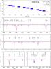 |
Fig. B.1 Spectral fit for N206-FS 66. |
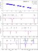 |
Fig. B.2 Spectral fit for N206-FS 111. |
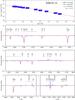 |
Fig. B.3 Spectral fit for N206-FS 131, which is suspected to be a binary (see Appendix A and next figure). |
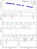 |
Fig. B.4 Composite model (red dashed line) for N206-FS 131. The primary Of star (brown dotted line) is fitted with T∗ = 38 kK model and secondary component (green dotted line) to a model with T∗ = 30 kK. See Table 3 for more information. |
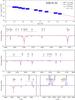 |
Fig. B.5 Spectral fit for N206-FS 162. |
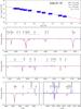 |
Fig. B.6 Spectral fit for N206-FS 178. |
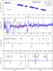 |
Fig. B.7 Spectral fit for N206-FS 180 with a single star model. The He i lines in the observation are absent in the model, indicating the contamination from a secondary component. See next figure for the composite model. |
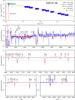 |
Fig. B.8 Composite model (red dashed line) for N206-FS 180 is the weighted sum of O2 V((f*)) (brown dotted line) and O8 IV (green dotted line) model spectra with effective temperature 50 kK and 32 kK, respectively. The relative offsets of the model continua correspond to the light ratio between the two stars. See Table 3 for more details. |
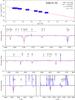 |
Fig. B.9 Spectral fit for N206-FS 193. |
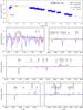 |
Fig. B.10 Spectral fit for N206-FS 214. The SED is best fitted to flux calibrated FUSE FUV spectra. The second panel shows the FUSE spectrum normalized with the model continuum. |
All Tables
Spectral type and coordinates of the nine Of-type stars in the N 206 superbubble.
Chemical abundance for the nine Of-type stars in the N 206 superbubble derived from spectral fitting.
All Figures
|
Fig. 1 Location of the Of-type stars in the N 206 H ii region. Three color composite image (Hα (red) + [O iii] (green) + [S ii] (blue)) shown in the background is from the Magellanic Cloud Emission-Line Survey (MCELS; Smith et al. 2005). The Of stars studied here are marked with the N206-FS number corresponding to Table 1. The dotted circle (blue) shows the rough locus of young cluster NGC 2018. The superbubble is located north-west and the SNR is at north-east of NGC 2018. |
| In the text | |
|
Fig. 2 Comparison of Hα lines of N206-FS 187 (O4 If) and neighboring star N206-FS 186 (O8.5 (V)e). |
| In the text | |
|
Fig. 3 Normalized spectra of the nine Of-type stars. The left panel depicts the medium resolution spectra in the blue (setting: LR02 and LR03). The high resolution spectra in the red (setting: HR15N) are shown in the right panelwhich includes Hα line. The central emission in Hα and the [O iii], [N ii], and [S ii] lines are from nebular emission (neb). |
| In the text | |
|
Fig. 4 Rotation velocity (ν sin i) from the line profile fitting of Of-type stars using the iacob-broad tool. The gray curves show the observed line profile. The ν sin i is calculated from line profile fitting based on Fourier transform method (red dotted line) and goodness-of-fit analysis (violet dashed line). See text for more details. |
| In the text | |
|
Fig. 5 Spectral fit for N206-FS 187. The upper panel shows the model SED (red) fitted to the available photometry from optical (UBV and I) and infrared (JHKs and IRAC 3.6 and 4.5 μm) bands (blue boxes) as well as the calibrated UV spectra from HST and IUE. The lower panels show the normalized HST and VLT-FLAMES spectra (blue solid line), overplotted with the PoWR model (red dashed line). The parameters of this best-fit model are given in Table 3. The observed spectrum also contains nebular emission lines (neb) and interstellar absorption lines (is). |
| In the text | |
|
Fig. 6 Models with different clumping parameters are compared to the P-Cygni profiles C iv λλ1548–1551 and N iv λ1718 of N206-FS 187 (blue solid line). Dashed lines (red) are for the model with Ṁ = 2.6 × 10⁻⁶M⊙ yr-1, D = 20, and RD = 0.05 R∗. The dotted lines (black) show the model with Ṁ = 1 × 10⁻⁵M⊙ yr-1, D = 10, and RD = 10 R∗. |
| In the text | |
|
Fig. 7 O v P-Cygni line profile of N206-FS 180 (blue solid line). Three models with different oxygen mass fractions (see labels) are shown for comparison. |
| In the text | |
|
Fig. 8 Effective temperature as a function of spectral type. Squares, triangles, and circles denote the luminosity classes Vz, V-IV, III-II and I, respectively. Typical uncertainties are indicated by the error bar in the upper left corner. |
| In the text | |
|
Fig. 9 Mass-loss rates vs. luminosity for the Of stars in the N 206 superbubble in the LMC. Open circles denote alternative values for the two supergiants obtained with stronger clumping (see Sect. 3.2.1). A power law is fitted to the data points. Symbols have the same meaning as in Fig. 8. The error bars are shown for each source. |
| In the text | |
|
Fig. 10 Modified wind momentum (Dmom) in units of M⊙ yr-1 km s |
| In the text | |
|
Fig. 11 Hertzsprung-Russell diagram for the nine Of stars in the N 206 superbubble in the LMC. The evolutionary tracks and isochrones are based on rotating (Vrot,init ~ 100 km s-1) evolutionary models presented in Brott et al. (2011) and Köhler et al. (2015). Different luminosity classes are denoted using rhombus, squares, triangles, and circles for luminosity class Vz, V-IV, III-II, and I, respectively. The position of the secondary components of N206-FS 131 and N206-FS 180 are also marked in the diagram with a cross symbol. |
| In the text | |
|
Fig. 12 Evolutionary masses compared to the spectroscopic masses. The discrepancy grows roughly linearly with the mass (see linear fit). The one-to-one correlation of spectroscopic and evolutionary masses is indicated by the dashed line. |
| In the text | |
|
Fig. 13 Surface nitrogen abundances as a function of the effective temperature. The downward arrow indicates an upper limit to the nitrogen abundance of N206-FS 111. |
| In the text | |
|
Fig. 14 Surface nitrogen abundances as a function of the projected rotation velocity ν sin i. The dashed line is a linear regression to the data. The downward arrow indicates an upper limit to the nitrogen abundance of N206-FS 111. |
| In the text | |
|
Fig. 15 Rate of ionizing photons as a function of the O subtype. |
| In the text | |
|
Fig. 16 Mechanical luminosity of stellar winds as a function of the O subtype. The open circles for the two supergiants refers to the models with alternative solution with higher clumping. Typical uncertainties are indicated with error bar in the upper right corner. |
| In the text | |
|
Fig. B.1 Spectral fit for N206-FS 66. |
| In the text | |
|
Fig. B.2 Spectral fit for N206-FS 111. |
| In the text | |
|
Fig. B.3 Spectral fit for N206-FS 131, which is suspected to be a binary (see Appendix A and next figure). |
| In the text | |
|
Fig. B.4 Composite model (red dashed line) for N206-FS 131. The primary Of star (brown dotted line) is fitted with T∗ = 38 kK model and secondary component (green dotted line) to a model with T∗ = 30 kK. See Table 3 for more information. |
| In the text | |
|
Fig. B.5 Spectral fit for N206-FS 162. |
| In the text | |
|
Fig. B.6 Spectral fit for N206-FS 178. |
| In the text | |
|
Fig. B.7 Spectral fit for N206-FS 180 with a single star model. The He i lines in the observation are absent in the model, indicating the contamination from a secondary component. See next figure for the composite model. |
| In the text | |
|
Fig. B.8 Composite model (red dashed line) for N206-FS 180 is the weighted sum of O2 V((f*)) (brown dotted line) and O8 IV (green dotted line) model spectra with effective temperature 50 kK and 32 kK, respectively. The relative offsets of the model continua correspond to the light ratio between the two stars. See Table 3 for more details. |
| In the text | |
|
Fig. B.9 Spectral fit for N206-FS 193. |
| In the text | |
|
Fig. B.10 Spectral fit for N206-FS 214. The SED is best fitted to flux calibrated FUSE FUV spectra. The second panel shows the FUSE spectrum normalized with the model continuum. |
| In the text | |
Current usage metrics show cumulative count of Article Views (full-text article views including HTML views, PDF and ePub downloads, according to the available data) and Abstracts Views on Vision4Press platform.
Data correspond to usage on the plateform after 2015. The current usage metrics is available 48-96 hours after online publication and is updated daily on week days.
Initial download of the metrics may take a while.