| Issue |
A&A
Volume 609, January 2018
|
|
|---|---|---|
| Article Number | A87 | |
| Number of page(s) | 23 | |
| Section | Interstellar and circumstellar matter | |
| DOI | https://doi.org/10.1051/0004-6361/201730834 | |
| Published online | 18 January 2018 | |
Connection between jets, winds and accretion in T Tauri stars
The X-shooter view⋆
1 INAF–Osservatorio Astronomico di Roma, via di Frascati 33, 00040 Monte Porzio Catone, Italy
e-mail: This email address is being protected from spambots. You need JavaScript enabled to view it.
2 INAF–Osservatorio Astronomico di Capodimonte, Salita Moiariello 16, 80131 Napoli, Italy
3 Scientific Support Office, Directorate of Science, European Space Research and Technology Centre (ESA/ESTEC), Keplerlaan 1, 2201 AZ Noordwijk, The Netherlands
4 INAF–Osservatorio Astrofisico of Arcetri, Largo E. Fermi, 5, 50125 Firenze, Italy
5 DIAS/School of Cosmic Physics, Dublin Institute for Advanced Studies, 31 Fitzwilliams Place, 2 Dublin, Ireland
6 INAF–Osservatorio Astrofisico di Catania, via S. Sofia 78, 95123 Catania, Italy
Received: 21 March 2017
Accepted: 28 September 2017
Abstract
Mass loss from jets and winds is a key ingredient in the evolution of accretion discs in young stars. While slow winds have been recently extensively studied in T Tauri stars, little investigation has been devoted on the occurrence of high velocity jets and on how the two mass-loss phenomena are connected with each other, and with the disc mass accretion rates. In this framework, we have analysed the [O i]6300 Å line in a sample of 131 young stars with discs in the Lupus, Chamaeleon and σ Orionis star forming regions. The stars were observed with the X-shooter spectrograph at the Very Large Telescope and have mass accretion rates spanning from 10-12 to 10-7M⊙ yr-1. The line profile was deconvolved into a low velocity component (LVC, | Vr | < 40 km s-1) and a high velocity component (HVC, | Vr | > 40 km s-1), originating from slow winds and high velocity jets, respectively. The LVC is by far the most frequent component, with a detection rate of 77%, while only 30% of sources have a HVC. The fraction of HVC detections slightly increases (i.e. 39%) in the sub-sample of stronger accretors (i.e. with log (Lacc/L⊙) >−3). The [O i]6300 Å luminosity of both the LVC and HVC, when detected, correlates with stellar and accretion parameters of the central sources (i.e. L∗, M∗, Lacc, Ṁacc), with similar slopes for the two components. The line luminosity correlates better (i.e. has a lower dispersion) with the accretion luminosity than with the stellar luminosity or stellar mass. We suggest that accretion is the main drivers for the line excitation and that MHD disc-winds are at the origin of both components. In the sub-sample of Lupus sources observed with ALMA a relationship is found between the HVC peak velocity and the outer disc inclination angle, as expected if the HVC traces jets ejected perpendicularly to the disc plane. Mass ejection rates (Ṁjet) measured from the detected HVC [O i]6300 Å line luminosity span from ~10-13 to ~10-7M⊙ yr-1. The corresponding Ṁjet/Ṁacc ratio ranges from ~0.01 to ~0.5, with an average value of 0.07. However, considering the upper limits on the HVC, we infer a Ṁjet/Ṁacc ratio < 0.03 in more than 40% of sources. We argue that most of these sources might lack the physical conditions needed for an efficient magneto-centrifugal acceleration in the star-disc interaction region. Systematic observations of populations of younger stars, that is, class 0/I, are needed to explore how the frequency and role of jets evolve during the pre-main sequence phase. This will be possible in the near future thanks to space facilities such as the James Webb space telescope (JWST).
Key words: stars: low-mass / line: formation / ISM: jets and outflows / accretion, accretion disks
Based on Observations collected with X-shooter at the Very Large Telescope on Cerro Paranal (Chile), operated by the European Southern Observatory (ESO). Programme IDs: 084.C-0269, 084.C-1095, 085.C-0238, 085.C-0764, 086.C-0173, 087.C-0244, 089.C-0143, 090.C-0253, 093.C-0506, 094.C-0913, 095.C-0134 and 097.C-0349.
© ESO, 2018
1. Introduction
The evolution and dispersal of circumstellar discs is an important step in the star and planet formation process. Disc dissipation in the first stages of pre-main sequence (PMS) evolution occurs due to the simultaneous effects of mass accretion onto the star and the ejection of matter from the star-disc system. Mass loss, in particular, follows different routes, that involve stellar winds, slow disc-winds, both photo-evaporated and magnetically driven, and high velocity and collimated jets. The latter are the most spectacular manifestation of mass loss phenomena, as they often extend over large spatial scales interacting with the ambient medium and originating the well known chains of shock spots known as Herbig-Haro objects (e.g. Bally 2016, and references therein). It is widely accepted that proto-stellar jets originate from the surface of accretion discs via a magneto-centrifugal launching mechanism. They are observed over the entire PMS life of a solar type star, from the embedded class 0 phase to the class II phase (Frank et al. 2014).
It is indeed a common paradigm that jets are a ubiquitous phenomenon during the active phase of accretion, as they are able to efficiently extract angular momentum accumulated in the disc, allowing matter in the disc to accrete onto the star. Millimetre observations of class 0 sources confirm that bipolar outflows and jets are ubiquitous at this evolutionary stage and represent a fundamental output of the star formation process (e.g. Mottram et al. 2017; Nisini et al. 2015). The role of jets in more evolved sources is less clear, although powerful optical jets are commonly observed in very active Classical T Tauri (CTT) stars. Due to the low extinction, they have been studied in details employing diagnostics based on line emission in a wide spectral range, from X-ray to IR wavelength (see e.g. Frank et al. 2014, and references therein). In few cases there is evidence that jets can efficiently extract the angular momentum, confirming their importance in mediating the accretion of matter from the disc onto the star (e.g. Bacciotti et al. 2002; Coffey et al. 2007). However, the frequency of the jet phenomenon among the general population of class II stars is still far from being settled. Searches for shocks and outflows through deep optical and IR imaging have been performed in several nearby star-forming regions, such as Lupus and Chamaeleon, and they have revealed the presence of only few tens of distinct flows (e.g. Bally et al. 2006; Wang & Henning 2009) against populations of more than 200 Young Stellar Objects (YSO; Luhman 2008; Evans 2009). This number represents however a lower limit on the jet occurrence in T Tauri stars, as for most sources the presence of a small-scale micro-jet could escape detection in large surveys with poor spatial resolution. The question on how common jets are in active accreting stars has a major relevance in the context of disc evolution, as jets can significantly modify the structure of the disc region involved in the launching with respect to a standard model that assumes only turbulence as the main agent for angular momentum dissipation (e.g. Combet & Ferreira 2008). In addition, jets can shield stellar radiation from reaching the disc surface, again altering the properties of the upper disc layers.
A direct way to infer the presence of high velocity gas in poorly embedded young stars is through observations of optical atomic forbidden lines, which are excited in the dense and warm shocked gas along the jet stream. Several surveys of forbidden lines in CTT stars have been so far conducted, mostly directed towards the bright sources of the Taurus-Auriga star forming region (e.g. Hamann 1994; Hartigan et al. 1995, henceforth H95, Hirth et al. 1997; Antoniucci et al. 2011; Rigliaco et al. 2013; Simon et al. 2016), and recently on a sample of sources in the Lupus and σ Ori regions (Natta et al. 2014, henceforth N14). Such surveys have in particular shown that the [O i]6300 Å transition is the brightest among the forbidden lines due to the combination of oxygen large abundance and favourable excitation conditions in the low ionization environment of the outflow.
The [O i]6300 Å line commonly exhibits two distinct components, as originally recognized in the pioneering work of Edwards et al. (1987): a low velocity component (LVC), peaking at velocities close to systemic one or only slightly blue-shifted, and a high velocity component (HVC) observed at velocities up to ~±200 km s-1. The origin of the LVC is still unclear, but it is quite well established that it comes from a distinct and denser region with respect to the HVC (H95, N14). The fact that the LVC is often blueshifted by up to 30 km s-1 indicates that it is associated with an atomic slow disc-wind, although a contribution from bound gas in Keplerian rotation in the inner disc has been suggested by recent observations at higher resolution (Rigliaco et al. 2013; Simon et al. 2016). The two main mechanisms invoked to explain the formation of slow disc-winds are photoevaporation of the gas in the disc by means of EUV/X-ray stellar and/or accretion photons (the so-called photoevaporative winds, Owen et al. 2010; Gorti et al. 2009) or winds driven by the magnetic field threading the disc (the magneto-hydro-dynamic, MHD, disc-winds, i.e. Casse & Ferreira 2000; Bai et al. 2016). As photoevaporation has been recognized to be an important mechanism for disc dispersal in late stages of PMS evolution (e.g. Alexander et al. 2014), great efforts have been given to model line excitation and profiles of the LVC in this framework (Ercolano & Owen 2010, 2016).
The HVC on the other hand can be directly connected with the extended collimated jets, as shown by long-slit spectroscopy performed along the flow axis in known jet driving sources. H95 was the first to use the HVC [O i]6300 Å luminosity in CTTs of the Taurus-Auriga clouds to measure the jet mass flux rate (Ṁjet) and estimate its ratio with the mass accretion rate (Ṁjet/Ṁacc ratio) in a sample of 22 sources. This is a fundamental parameter that characterizes the jet efficiency in regulating the mass transfer from the disc to the star. Subsequent studies have revised the Ṁacc determinations on some of the H95 sources adopting different methods (e.g. Gullbring et al. 1998; Muzerolle et al. 1998), suggesting that the Ṁjet/Ṁacc ratio in the sample of Taurus sources spans between ~0.05 and 1. Determinations of this ratio as derived from detailed studies of individual jets agree with these values in a wide range of masses, and for young and embedded sources (Cabrit 2007; Antoniucci et al. 2008, 2016). All these estimates suffer, however, from the non-simultaneous determination of the accretion and ejection parameters, or from different adopted methods and assumptions. Consequently, it is not clear whether the large scatter in the derived ratio is due to the non-homogeneity of the approach or to a real effect. An adequate answer to this problem can be given only by applying the same methodology to a statistically significant sample of sources where accretion and ejection tracers are simultaneously observed.
Details on the used X-shooter samples.
In this paper, we present an analysis conducted on a sample of 131 class II sources (mostly CTT stars) in the Lupus, Chamaeleon and σ Orionis star-forming regions, whose UV and optical spectra have been acquired with the X-shooter instrument (Vernet et al. 2011) at the Very Large Telescope (VLT). These observations are part of a project aimed at characterizing the population of YSO with discs in nearby star-forming regions (Alcalá et al. 2011). As part of this project, the stellar and accretion parameters of the observed stars have been consistently and uniformly derived (Rigliaco et al. 2012; Alcalá et al. 2014, 2017; Manara et al. 2016a, 2017; Frasca et al. 2017). The same sample of Lupus observed with X-shooter has been also observed with ALMA (Ansdell et al. 2016) and the inferred disc masses were found to be correlated with the mass accretion rates (Manara et al. 2016b). For a sub-sample of these sources, the HI line decrements have been analysed and the general properties of the hydrogen emitting gas derived (Antoniucci et al. 2017).
A study of the forbidden line emission in a sub-sample of 44 sources in Lupus and σ Orionis is presented in N14. These authors concentrated their analysis on the properties of the LVC and derived correlations between the LVC luminosity and accretion and stellar luminosities. In addition, ratios of different lines showed that the LVC originates from a slow dense wind (ne> 108 cm-3) which is mostly neutral. Here we extend the work of N14 to a much larger sample of objects covering a wider range of stellar and accretion properties. Our work is, however mainly focussed on the HVC and aims at investigating the occurrence of jets during the class II phase, measuring the jet efficiency and studying whether it varies with the source properties. In addition, relationships between the LVC and HVC will be also discussed, with the goal of defining any connection between the phenomena giving rise to the two emissions.
The paper is organized as follows: Sect. 2 presents the data sample adopted for our analysis. In Sect. 3 we describe the procedure adopted to retrieve the parameters of the LVC and HVC from the [O i]6300 Å line profiles, while Sect. 4 summarizes the statistics on the detection of the two components. In Sects. 5 and 6 correlations between the [O i]6300 Å luminosity and stellar and accretion parameters are derived and the Ṁjet/Ṁacc ratio discussed. Section 7 describes kinematical information on the HVC and LVC derived from line profiles. Discussion and conclusions are finally presented in Sects. 8 and 9, respectively.
2. The data sample
The adopted sample consists of 131 YSOs observed with the X-shooter instrument. In particular, the sample includes sources in the Lupus, Chamaeleon and σ Orionis star forming regions, whose X-shooter spectra have been already analysed in previous papers (Alcalá et al. 2014 and 2017 for Lup; Rigliaco et al. 2012 for σ Ori; Manara et al. 2016a and 2017 for Cha). Details on observations and data reduction are given in those papers while Table 1 summarizes the instrument setting for each sub-sample of sources.
The Lupus sources comprise 82 confirmed YSOs of the Lupus I, II, III, IV clouds, and constitute the most complete and homogeneous sub-sample analysed in this work. They, in fact, represent about 90% of all the candidate class II in these clouds. Thirty-six of these sources have been observed as part of the INAF/GTO X-shooter programme while the remaining 40 are part of two individual follow-up programmes (095.C-0134 and 097.C-0349, P.I. J. Alcalá). The two samples were observed with the same X-shooter setting, but the spectral resolution of the more recently acquired sample is slightly lower (~7500 vs. 8800 in the VIS arm) due to a change of the instrument slit wheel between the two sets of observations. We have also included ESO archival data for six additional sources (see Alcalá et al. 2017), that have been observed with a narrower slit at a higher resolution (~18 000).
The Chamaeleon sample comprises 25 of the accreting sources analysed in Manara et al. (2016a) plus 16 sources observed in the programme 090.C-0253 (P.I. Antoniucci) for a total of 41 objects (31 in Cha I and 10 in Cha II). These observations were all performed at the highest X-shooter resolution (see Table 1). All the considered Cha I sources are part of the larger sample presented in Manara et al. (2017) while the Cha II objects are presented here for the first time. The derived stellar and accretion parameters for these additional sources are discussed in Appendix A and summarized in Table A.1. Finally, we have also included in the sample the eight sources in the σ Ori cloud studied in Rigliaco et al. (2012) and Natta et al. (2014).
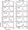 |
Fig. 1 Examples of [O i]6300 Å spectra of sources with and without a HVC. Blue-dashed lines indicate the Gaussian profiles used to fit the different components, and the red-dashed line is the final best fit. |
The stellar and accretion parameters (namely L∗, extinction, spectral type, Lacc) of all stars have been self consistently derived by fitting the X-shooter spectrum with the sum of a stellar photosphere and an excess continuum due to accretion (see Alcalá et al. 2017 and Manara et al. 2016a for details). Stellar mass depends on the adopted evolutionary tracks, and we adopt here masses derived from the Baraffe et al. (2015) tracks for all samples, with the exception of the σ Ori objects whose masses have been derived by Rigliaco et al. (2012) from the Baraffe et al. (1998) tracks. Accretion luminosities were eventually converted into mass accretion rates (Ṁacc) using the relation Ṁacc , where R⋆, the stellar radius, was calculated from the effective temperature and stellar luminosity (for more details see, e.g. Alcalá et al. 2014).
The list of considered sources is given in Table B.1. Given the slightly different setting for the Lupus observations, we maintained the division in three different sub-samples (GTO, New sample, Archive) as done in Alcalá et al. (2017). For convenience, the table also reports all the relevant parameters collected from the individual papers. Considering the global sample, masses range between 0.02 and 2.13 M⊙, log (Lacc/L⊙) between −5.2 and +0.85, and the corresponding mass accretion rates are between ~10-12 and 10-7M⊙ yr-1, meaning that they span approximately five orders of magnitude.
The majority of the sources of our global sample are class II CTTs. The sample also includes a small group (12) of transitional discs (TD) in Lupus, that is, T Tauri sources having discs with large inner holes depleted of dust. In addition, the sample includes 14 sources with mass ≲0.1 M⊙, thus comprising possible brown dwarf (BD) candidates. We will discuss the properties of these stars separately in the following analysis as their accretion and ejection properties might be different from those of CTT stars.
Finally, on the basis of the derived stellar parameters, seven sources in Lupus have been classified as “sub-luminous”, that is they have a stellar luminosity much lower than that of the other sources of the cloud with the same spectral type. They are likely to be sources with the disc seen edge-on, hence partially scattering the stellar continuum. Two of these sources (namely Sz133 and Sz102 in Lupus) fall below the zero-age main sequence and thus an estimate of the mass (and mass accretion rate) was not obtained (Alcalá et al. 2017). Finally, six sources in Lupus have an accretion rate compatible with chromospheric emission and thus their Lacc value has been considered here as an upper limit. All the above cases are indicated in the notes of Table B.1.
3. [O i] profile decomposition
We focussed our analysis on the [O i]6300 Å line which is the brightest among the class II forbidden lines in the spectral range of our data (e.g. H95, N14). The [O i]6300 Å emission of the Lupus stars observed in the GTO and σ Ori sample has been analysed and discussed in N14 together with the emission from other forbidden lines. We have applied the same methodology as in N14 to the rest of the sample in order to have an homogeneous database of [O i] luminosities in the different kinematical components.
As discussed in the introduction, the [O i]6300 Å profile can be decomposed in a LVC, close to systemic velocity, and a blue- or red-shifted HVC. To separately derive line center and width of the different components we fitted the [O i] line profile with one or more Gaussians. We have used the photospheric rest velocity as measured from the Li i line at 6707.876 Å to set the zero velocity scale of all spectra. For the few cases in which the Li i line was not detected, we used the K i photospheric line at 7698.974 Å.
Given the limited spectral resolution, we did not attempt fits with more than three Gaussians (one for the LVC and two for the blue- and red-shifted components of the HVC). To be consistent with N14, we defined the velocity that separates the LVC from the HVC as 40 km s-1, which roughly corresponds to the resolution attained for most of the Lupus objects. However, the resolution of the observations in Chamaeleon is higher by approximately a factor of two, so we are potentially able to identify HVC even if at lower radial velocities. For this sample we consistently defined any emission with peak radial velocity | Vr | < 40 km s-1 as an LVC if a single component is detected. However, if we detected two components, the one at the higher velocity was defined as HVC even if it has a | Vr | < 40 km s-1.
We remark that this second component could not be associated to a jet, but rather to the broad, slightly blue-shifted LVC component with | Vr | typically of ≲30 km s-1 sometimes detected in high resolution observations (e.g. Rigliaco et al. 2013; Simon et al. 2016). Since there are only four of such cases in our sample, this distinction is not going to affect our statistics.
To perform the deconvolution, we have used the onedspec task within the IRAF1 package. The HVC component can be identified as an individual line (often partially blended with the LVC) or as an extended (mostly blue-shifted) wing of the LVC (see Fig. 1 for some examples). In this latter case, as the result of the deconvolution might be more dependent on the initial guess for the Gaussian parameters, we have checked the IRAF deconvolution also using the curve-fitting programme PAN (Peak-analysis) within DAVE (Data Analysis and Visualization Environment), running on IDL (Azuah et al. 2009). This programme allows one to define the initial guess not only on the velocity peak but also on the width of the Gaussians, as well as to have better visualization of the individual fitted curves. We find in all cases that a different choice of the initial parameters influences the final deconvolved line flux by no more than 30%. The largest uncertainty on the peak velocities is estimated to be about 5 and 10 km s-1 for the LVC and the HVC, respectively. When the HVC is not detected, a 3σ upper limit is derived from the rms of the continuum computed in regions adjacent to the LVC, multiplied for the instrument resolution element.
Line fluxes have been corrected for extinction and then converted into intrinsic luminosities adopting the AV and distances values given in Table B.1. All the derived line parameters are listed in Table B.2, where we report, in addition to the new determinations, also the [O i]6300 Å line parameters relative to the Lupus and σ Ori GTO sample published in N14.
The detection frequency of other forbidden lines tracing the HVC (e.g.[S ii] 6716.4, 6730.8 Å and [N ii] 6548.0, 6583.4 Å) is always lower than that of the [O i]6300 Å line, and their signal-to-noise ratio (S/N) usually worse, therefore we do not discuss them in this paper. However, for sources where the [S ii] and [N ii] lines are detected with a good enough S/N we have performed the Gaussian decomposition into a LVC and HVC and checked that the resulting kinematical parameters are consistent with those of the [O i]6300 Å lines. Appendix C summarizes the peak velocities and full width at half maximum (FWHM) derived in these cases, which generally agree with those derived for the [O i]6300 Å line within ~±20 km s-1.
We have also examined the X-shooter 2D spectral images to see if spatially extended [O i]6300 Å emission can be resolved in sources where the HVC component is detected, due to a fortuitous alignment of the instrumental slit with the jet axis. We found that in five of the brightest [O i]6300 Å sources the HVC emission peak is shifted with respect to the source continuum by ~0.̋2–0.̋4. The position velocity (PV) diagrams relative to these sources are presented in Appendix D. In one of the sources, Sz83, the HVC appears composed by at least four different emission peaks at different velocities, showing an increase in the spatial displacement with increasing speed. This jet acceleration pattern was already found and studied with spectro-astrometric techniques by Takami et al. (2001). Finally, one of the sources with strong HVC emission, Sz102, is a well known driver of an optical jet (Krautter 1986). We do not detect any appreciable shift in its emission as the used X-shooter slit was aligned perpendicular to the jet axis.
4. Statistics
The [O i]6300 Å line is detected in 101 out of the 131 sources of our sample (i.e. 77% rate of detection). In all detections the LVC is identified, while the HVC is observed in 39 of the 131 objects (i.e. 30% rate of detection). These detection rates are similar to what is found in N14 for the authors’ limited sample of 44 sources (84% and 27% detections for the [O i]6300 Å LVC and HVC, respectively). The L[O i] HVC spans a wide range of values – between 0.01 and 3 L⊙ – for the detections. In the majority of the sources the L[O i] HVC is typically fainter than the L[O i] LVC by a factor of two or three, which partially explains the higher number of LVC detections with respect to the HVC. However sensitivity alone is not the only reason for a difference in detection rate between the LVC and HVC, as the S/N in the LVC line is often larger than 10. In some of the sources orientation effects could misclassify emission at high velocity with a LVC. Assuming a total jet maximum velocity of 200 km s-1 (see Sect. 7) any jet inclined by less than 78 degree with respect to the line of sight would have a Vrad > 40 km s-1 and thus will be detected by us as a HVC. The probability that a jet in a randomly oriented sample of stars has a line-of-sight inclination angle <θdeg is P( <θ) = 1−cos(θ). For θ = 78deg, the probability is 80% which means that in 20% of the sources (~25 sources) a high velocity jet could be in principle misinterpreted as a LVC. This number is probably lower as observations of Chamaeleon objects were performed at higher resolution, thus in principle able to better identify HVC emission at lower radial velocity in this sub-sample. Even taking this effect into account, we still do not detect the HVC in about 50% of sources potentially with favourable inclination.
Non-detection due to orientation effects might be more important for BD and very low mass objects as the total jet velocity depends on the stellar mass, hence the jet radial velocity in these sources might be comparable to our velocity threshold. Indeed BD jets have Vr typically less than 40 km s-1 even for low inclinations with respect to the line of sight (e.g. Whelan et al. 2014). Among the 14 sources of our sample with M∗ less than 0.1 M⊙, only two have a detected HVC (20% of sources). If we exclude these sources from our statistics, the total detection rate increases to 32%.
Our detection rates can be compared with those of similar studies performed at higher spectral resolution, thus potentially less affected by orientation effects. For example, Simon et al. (2016) observed the [O i]6300 Å line in a sample of 33 YSO with a resolution of 6.6 km s-1 detecting HVC emission in 13 sources, thus with a detection rate of 39%, similar to our study. On the other hand the HVC was detected in 25 out of the 42 sources of H95, a detection rate of ~60%. This different detection rate could be related, in addition to the higher resolution, also to the different properties, mass and mass accretion rates in particular, of the H95 sources in comparison with those of our sample.
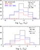 |
Fig. 2 Distribution of accretion (top) and stellar (bottom) luminosity for all the sources of our sample is depicted in black. Red and blue histograms are relative to sources where the HVC has been detected and not-detected respectively. In the upper corner of each plot the percentage of HVC detection in two ranges of luminosities is indicated. |
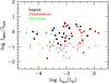 |
Fig. 3 Ratio between the HVC and LVC [O i]6300 Å line luminosities as a function of the accretion luminosity. Black, red and green symbols indicate sources in Lupus, Chamaeleon and σ Orionis clouds, respectively. Arrows refer to 3σ upper limits for the HVC luminosity. |
To explore for any dependence of the HVC detection with source parameters, in Fig. 2 we show the distribution in Lacc and L∗ separately for sources where the HVC has been detected and not-detected. It can be seen that detections are not segregated in specific ranges of parameters. However, there is a clear trend for higher detection rates in sources with higher Lacc. For example, the detection rate decreases from 39% in sources with log (Lacc/L⊙) >−3 to 11% in sources with log (Lacc/L⊙) ≤−3. This trend explains the lower rate of HVC detection in the N14 sample with respect to our enlarged sample, which contains a larger number of sources with higher accretion luminosity. No significant variation in the detection rate is instead observed in sources with different stellar luminosity: stars with log (L∗/L⊙) <−1 show a similar detection rate as the stars with higher luminosity.
Figure 3 displays the ratio between the HVC and LVC line luminosity as a function of the accretion luminosity. When a HVC is detected the luminosity ratio varies between ~0.1 and 4, with most of the sources having a L[O i] LVC luminosity equal or lower than the L[O i] HVC . No dependence with Lacc is found.
Of the 11 TD of our sample all but two have a LVC, while two of them (namely Sz100 and Sz123B) have also a HVC. These numbers are roughly in line with the overall statistics of our sample (i.e. 80% LVC, 20% HVC), and consistent with the fraction of TD with [O i] LVC in the study of Manara et al. (2014). This evidence confirms that TD have characteristics similar to other CTTs with a full disc, not only for what accretion properties concern (Manara et al. 2014; Espaillat et al. 2014), but also regarding the properties of the inner atomic winds. Moreover, the detection of the HVC in two of them, in the assumption that this component traces a collimated jet, indicates that these sources are undergoing magnetospheric accretion. Finally, of the six sources whose permitted line emission is more consistent with chromospheric activity rather than with accretion activity, only Lup607 shows [O i] emission in a LVC.
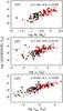 |
Fig. 4 [O i]6300 Å line luminosity of the LVC is plotted as a function of, from top to bottom, stellar mass, stellar luminosity and accretion luminosity. Colour codes for the symbols are as in Fig. 3. Arrows refer to 3σ upper limits. The dashed line indicates the linear regression whose parameters are given in the upper right corner of each figure, together with the correlation parameter. |
5. Correlation with stellar and accretion parameters
The [O i]6300 Å line luminosity has been correlated with the stellar and accretion parameters for both the LVC and HVC. Results are shown in Fig. 4 (L[O i] LVC vs. Lacc, L∗ and M∗), Fig. 5 (L[O i] HVC vs. Lacc, L∗ and M∗), and Fig. 6 (L[O i] LVC and L[O i] HVC vs. Ṁacc). The line luminosity correlates well with all the considered parameters in both LVC and HVC as shown by the Pearson correlation coefficient r displayed in each plot, which is always between 0.7 and 0.8, with the exception of the L[O i] HVC vs. L∗ correlation whose coefficient is 0.63. In the L[O i] LVC vs. L∗ plot we indicate the locus of the two sub-luminous sources (namely ParLup 3-4 and Sz102) that significantly deviate from the correlation found for the other sources. Given the uncertainty of their stellar luminosity, we have not included them in deriving the correlation parameters. Finally, we have checked that the correlations do not change if we exclude the TD sources from our sample.
We performed a best fit linear regression finding the following relationships: log(L[O i] LVC) = (0.59 ± 0.04)log Lacc + (−4.13 ± 0.11) log(L[O i] LVC) = (1.06 ± 0.11)log L∗ + (−4.65 ± 0.10) log(L[O i] LVC) = (1.87 ± 0.13)log M∗ + (−4.52 ± 0.08) log(L[O i] LVC) = (0.68 ± 0.05)log Ṁacc + (0.69 ± 0.50)
and log(L[O i] HVC) = (0.75 ± 0.08)log Lacc + (−4.03 ± 0.17) log(L[O i] HVC) = (1.22 ± 0.21)log L∗ + (−4.54 ± 0.18) log(L[O i] HVC) = (2.13 ± 0.29)log M∗ + (−4.48 ± 0.16) log(L[O i] HVC) = (0.79 ± 0.10)log Ṁacc + (1.50 ± 0.86). We found a slightly flatter slope for the L[O i] LVC vs. L∗ and L[O i] LVC vs. Lacc correlations with respect to N14 (i.e. 1.37 ± 0.18 and 0.81 ± 0.09, respectively). Our L[O i] LVC vs. Lacc has a slope more similar to that found by Rigliaco et al. (2013) in a sample of Taurus sources (0.52 ± 0.07). We point out that the present sample includes sources with higher Ṁacc than the N14 sample alone, which could be at the origin of the different slope. Correlations with L∗ present the larger scatter and in general we find that both the LVC and HVC show a better correlation with Lacc than with all the other parameters.
Mendigutía et al. (2015) investigated the nature of the known correlations between accretion and emission line luminosities. They argue that such correlations cannot be directly attributed to a physical connection between the line formation region and the accretion mechanism since they are mainly driven by the fact that both accretion and line luminosity correlate with the luminosity of the central source. They suggested to use luminosities normalized by L∗. This is what we show in Fig. 7, where the L[O i]/L∗vs. Lacc/L∗ correlation is plotted for both the LVC and HVC. We see that [O i]6300 Å line to stellar luminosity ratio is still correlated with the accretion to stellar luminosity ratio, supporting the idea that the physical origin of the line is, directly or indirectly, related to the accretion mechanism. The same conclusion is also suggested by Frasca et al. (2017), who found that their derived Hα line fluxes per unit surface in the sources of the Lupus sample tightly correlate with accretion luminosity, excluding any influence from calibration effects.
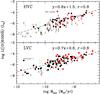 |
Fig. 6 [O i]6300 Å line luminosity of the LVC (bottom) and HVC (top) is plotted as a function of the mass accretion rate. Symbols and labels are as in Fig. 4. |
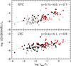 |
Fig. 7 Correlations between the [O i]6300 Å line and accretion luminosities, both normalized by the stellar luminosity. Symbols and labels are as in Fig. 4. |
Correlations between [O i] luminosity and mass accretion rate or accretion luminosity have already been found, and used to derive the mass accretion rate in sources where Balmer jump or permitted line luminosities were not detected or uncertain (e.g. Herczeg et al. 2008). This is however the first time that such correlations are separately found for the LVC and HVC. The log(L[O i] HVC) vs. log Ṁacc correlation is particularly useful to indirectly estimate the mass accretion rate in moderately embedded sources driving jets, where the permitted lines or the LVC emission region might be subject to large extinctions or scattering (e.g. Nisini et al. 2016).
The derived L[O i] LVC vs. Lacc luminosity relationships can be additionally used to indirectly estimate the accretion luminosity in the sub-luminous sources. The Lacc measured in these sources from the UV excess could be underestimated due to the fact that part or most of the UV radiation is scattered away by the edge-on disc. On the contrary, the [O i]6300 Å emission originates mostly from a more extended region above the disc surface, thus it is less affected by the disc obscuration (see e.g. Whelan et al. 2014). Figure 8 displays the comparison between the two Lacc determinations for the five sub-luminous objects where [O i]6300 Å emission has been detected. In only two of them, namely Par-Lup 3-4 and Sz102, the Lacc derived from L[O i] LVC is significantly larger (up to two order of magnitudes) than the value estimated from the UV excess. We note that extended optical jets have been detected in these two sources (Whelan et al. 2014; Krautter 1986), therefore their [O i]6300 Å emission should be the least contaminated by disc obscuration.
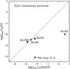 |
Fig. 8 Accretion luminosity derived by modelling the UV excess is compared with that estimated through the L[O i] LVC vs. Lacc relationships for the sub-luminous sources. |
6. Mass ejection rate and its connection with mass accretion
In the assumption that the [O i]6300 Å HVC traces the high velocity jet, its luminosity can be converted into the total mass in the flow (M) given that forbidden lines are optically thin. The jet mass flux rate can be then estimated as Ṁjet = M × V/l, where V is the flow speed and l is the scale length of the considered emission. For our calculation we considered V/l = V⊥/l⊥, where V⊥ is the component of the velocity projected on the plane of the sky, and l⊥ is the projected scale length of the emission. We took V⊥ to be equal to 100 km s-1, assuming a total jet velocity of 150 km s-1 and a median inclination angle of 45° (see also Sect. 7), and l⊥ equal to the size of the aperture at the given distance (see H95).
To measure the mass of the flow from the line luminosity we have considered the [O i]6300 Å emissivities computed considering a five-level O i model, and assuming Te = 10 000 K and ne = 5 × 104 cm-3. This choice is based on the values that typically represent the region at the base of T Tauri jets, where the [O i] emission originates. In particular, we have considered values estimated from multi-line analysis that include also the [O i]6300 Å line, as in H95, or from the analysis of [Fe ii] lines, that have excitation conditions similar to [O i] (Giannini et al. 2013). The adopted values are also similar to those used by H95 to estimate the Ṁjet of a sample of Taurus sources from their HVC [O i] emission. Hence, we can make a direct comparison between our derived mass flux rates and those estimated by H95. We further assumed that oxygen is neutral with a total abundance of 4.6 × 10⁻⁴ (Asplund et al. 2005). This hypothesis is supported by the absence of, or presence of very weak [O ii] emission in our spectra (see also N14).
The spread in the density and temperature values among different objects is the major source of uncertainty on the derived Ṁjet. In particular, the [O i] emissivity scales with the density for ne ≲ 106 cm-3. Estimates done on CTT jets base indicate that ne roughly varies in the range 2−6 × 104 cm-3 and Te might be between 7000–15 000 K (e.g. Agra-Amboage et al. 2011; Maurri et al. 2014; Hartigan et al. 2007; Giannini et al. 2013). Considering the emissivity variations in this range of values, and including a factor of two of uncertainty on the tangential velocity, this leads to a cumulative uncertainty on Ṁjet of about a factor of ten. We remark that electron density and temperature values measured in different jets do not show any dependence on mass or mass accretion rate of the central stars, being similar in actively accreting solar mass objects, as well as in brown-dwarfs and very low mass stars (e.g. Whelan et al. 2009; Ellerbroek et al. 2013). This circumstance reassures us that we do not introduce a bias by assuming the same physical parameters for all sources of our sample.
In deriving the mass flux rate, we have summed up both the red-shifted and blue-shifted components when detected. In most of the cases the red-shifted component is not detected, likely because the receding flow is occulted by the disc. To take into account this observational bias, we have multiplied by two our derived Ṁjet in all the cases where only the blue-shifted component is detected. An upper limit on the double-sided Ṁjet have been also estimated from the upper limits on the L[O i] HVC multiplied by two to correct for the flow bipolarity.
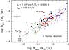 |
Fig. 9 Mass accretion (Ṁacc) vs. mass ejection (Ṁjet) rates. The mass ejection has been measured from the [O i]6300 Å luminosity assuming a jet tangential velocity of 100 km s-1 and gas temperature and density of 10 000 K and 5 × 104 cm-3 respectively. Black, red and green symbols are as in Fig. 4, while blue triangles indicate the values for the sample of Taurus sources of H95. Updated mass accretion rates from these sources are estimated from the data in Rigliaco et al. (2013). Average data point uncertainty is indicated with a cross on the left side of the plot. Arrows refer to upper limits on Ṁjet derived from the 3σ upper limits on the L[O i] HVC luminosity. |
In Fig. 9 the derived mass flux rates are plotted as a function of the source mass accretion rates. To guide the eye, lines corresponding to Ṁjet/Ṁacc ratio between 0.01–0.5 are drawn in the figure.
In Fig. 9 we also plot the data points relative to the sample of sources in Taurus whose Ṁjet has been measured by H95 with a similar procedure as the one we adopt here. In H95 the authors measured the accretion rate from the source veiling, but these values were lately found to overestimate the true values (Gullbring et al. 1998). Several determinations of the mass accretion rate of the H95 sample are available in the literature. For the plot, we have used the determination of the accretion luminosity given by Rigliaco et al (2013) which derived it from the Hα luminosity measured on the same data-set of H95. We have then converted Lacc into Ṁacc by adopting the stellar masses and radii given in Rigliaco et al. (2013). The Taurus sources, which extend to higher mass accretion rates with respect to our sample, fall along the same trend as the rest of targets.
The figure shows that for most of the detections the Ṁjet/Ṁacc ratio is between 0.01 and 0.5, confirming, on a large statistical bases, previous results found on individual objects. Only one object, ESO-Hα 562, has a Ṁjet/Ṁacc ratio much larger than one. This source is a close binary with two components of the same spectral type but with different extinction values (AV = 4 and 10 mag, Daemgen et al. 2013). It is therefore possible that the mass accretion rate, estimated from the UV excess, refers only to the less extincted of the two stars while the mass ejection rate is the sum of the two contributions (see discussion in Appendix 3.1 of Manara et al. 2016a).
We note a significant number of upper limits pointing to a very low efficiency of the jet mass loss rate, even for objects with high accretion rates. This is better visualized in Fig. 10, which shows an histogram with the distribution of the estimated Ṁjet/Ṁacc ratio, dividing detections and upper limits. Here the Taurus sources are not included. The peak in the detections is at Ṁjet/Ṁacc = 0.07, with 13/39 (i.e. 33%) of sources in the range 0.03 and 0.1. Considering both detections and upper limits, however, we find that 57 sources, (44% of the entire sample), have Ṁjet/Ṁacc< 0.03.
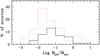 |
Fig. 10 Distribution of ejection efficiency (Ṁjet/Ṁacc) for the global sample. Black histogram are values for sources with detected HVC while red dotted histogram indicates the distribution of upper limits. |
The large scatter in the Ṁjet/Ṁacc ratio is partially due to the uncertainty in the determination of the Ṁjet, and in particular on the assumed parameters. However, given the remarkable similarity in the excitation conditions of jets from sources with different masses and mass accretion rates, it is likely that the scatter, of almost two order of magnitude, reflects a real difference in the Ṁjet efficiency among sources more than excitation conditions very different from what assumed here. We also remark that the Ṁjet/Ṁacc ratios for the two TDs of our sample with detected HVC are 0.1 and 0.4, that is, in line with the other sources.
The dependence of the Ṁjet/Ṁacc ratio with the mass and mass accretion rate is presented in Fig. 11. Sources with Ṁacc between 10-10 and 10-8M⊙ yr-1 have Ṁjet/Ṁacc ratio that spreads all values between 0.01 and 1. Lower accretors with detected HVC have a ratio larger than 0.1, however the non detection of sources with lower values is likely due to sensitivity limits. Sources with higher mass accretion rates (i.e. >10-8M⊙ yr-1) have a tendency of displaying Ṁjet/Ṁacc ratio lower than 0.1. The sources in Taurus follow a similar trend with a few exceptions.
The upper panel of Fig. 11 shows that no dependence of the inferred ratio with M∗ is observed. Previous studies suggested that the Ṁjet/Ṁacc ratio may be higher in BDs than CTTSs (Whelan et al. 2009). In our sample most of sources with M∗≲ 0.1 M⊙ have upper limits that do not allow us to infer any particular trend for the Ṁjet/Ṁacc ratio.
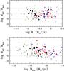 |
Fig. 11 Upper panel: log of the Ṁjet/Ṁacc ratio plotted as a function of the log of the stellar mass. The three horizontal dashed lines correspond to Ṁjet/Ṁacc = 1, 0.1 and 0.01. Black, red and green symbols are as in Fig. 4 while blue triangles refer to the sources in Taurus (see caption of Fig. 9). Lower panel: log of the Ṁjet/Ṁacc ratio plotted as a function of the log of the mass accretion rates. |
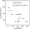 |
Fig. 12 Absolute value of the peak velocity in the HVC (Vpeak(HVC)) is plotted as a function of the disc inclination angle for a sub-sample of sources in Lupus where idisc has been measured from ALMA observations (Tazzari et al. 2017). Upper limits refer to sources with measured inclination angles that don’t have a HVC component. An upper limit of Vpeak(HVC) of 40 km s-1 has been considered in the plot for these sources. |
In conclusion, the analysis of Ṁjet/Ṁacc ratio shows that there is a large spread of values for this ratio that does not depend on the mass of the driving source. There is however a tentative trend for sources with accretion rates >10-8M⊙ yr-1 to have on average a lower ratio. This trend needs to be confirmed/rejected on the bases of observations on a more complete sample of sources with high mass accretion rates.
7. Peak velocities and dispersion
Our spectral resolution is too low to perform a comprehensive kinematical analysis of the observed lines. It is however sufficiently high for studying general trends related to the properties of the gas giving rise to the two velocity components.
An analysis of the dependence of the observed kinematical behaviour on the jet inclination with respect to the observer can be done for the sub-sample of the Lupus sources where a measure of the disc inclination angle is available. Ansdell et al. (2016) observed with ALMA the entire Lupus sample investigated here, and were able to spatially resolve the disc in 20 sources. The [O i]6300 Å line was detected in 13 of these resolved structures, nine of which show HVC emission. Tazzari et al. (2017) revisited the disc inclination angles provided by Ansdell et al. (2016) applying a more accurate fitting procedure of the visibilities. Here we used these determinations for our analysis. Figure 12 shows the HVC peak velocity (Vpeak(HVC)) plotted as a function of the disc inclination angle. The absolute value of the HVC radial projected velocity is anti-correlated with the disc inclination angle, as expected in the working hypothesis that the HVC traces collimated jets ejected in a direction perpendicular to the disc. In five of the sources where the inclination angle is available we do not detect a HVC. Two of them have high idisc values (namely Sz84: idisc = 72.9° and Sz133: idisc = 78.5°) and their position in the plot is compatible with the presence of a jet at low radial velocity. Of these sources, Sz84 has a small LVC width (ΔV = 23 km s-1) indicating that if any jet at low radial velocity is present in this source, its contribution to the overall line profile should be negligible. Sz133, on the other hand, has a wide [O i]6300 Å line (ΔV = 63.7 km s-1) which is compatible with a blended HVC at low radial velocity (see the relative line profile in Fig. 1).
If we de-project the peak velocities adopting the corresponding inclination angle, we find total velocities ranging between ~100 and 150 km s-1. Since we consider the peak of the [O i]6300 Å emission, these values represent the mean flow velocity. Appenzeller & Bertout (2013) found a similar correlation in a sample of T Tauri with known inclination angle, but considering the [O i]6300 Å maximum velocity computed at 25% of the line intensity. They found for their sample an average jet maximum velocity ~250 km s-1. They also performed the same analysis considering the peak velocity of the [N ii] lines finding jet mean velocities of the order of 200 km s-1, thus higher than typical values found by us. This could be related to the fact that the Appenzeller & Bertout (2013) sample is dominated by more massive sources in the Taurus cloud. Indeed, in magneto-centrifugally launched jets, the maximum poloidal velocity is roughly proportional to (rA/r0)vK, where r0 is the jet anchoring radius, rA is the Alfvén radius (i.e. the radius at which the flow poloidal velocity is equal to the Alfvén speed), and  is the Keplerian velocity in the disc at r0. The lower total jet velocities in the Lupus sources with respect to sources in Taurus could be therefore due to their average smaller stellar mass and consequently smaller Keplerian velocity and Alfvén radius (which in turn depends on the mass and stellar magnetic field). Our derived jet velocities are in fact more in line with the velocities found from proper motion analysis in a sample of jets of the Cha II cloud (Caratti o Garatti et al. 2009), driven by sources more similar to those investigated here in terms of stellar parameters.
We have also investigated whether there is any dependence among the HVC and LVC kinematics with the aim of disentagling the origin of the LVC component. To this aim, Fig. 13 shows the correlation between Vpeak(HVC) and the line width (ΔV) of the LVC. The line width has been obtained from the FWHM of the fitted Gaussian, deconvolved for the instrumental profile  . Sources where the observed line width is smaller than the instrumental resolution are excluded. If the LVC emission is dominated by gravitationally bound gas in the disc, we should observe an anti-correlation between Vpeak(HVC) and ΔV(LVC), since a progressively larger spread in disc radial velocities is seen as the disc inclination increases.
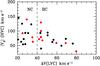 |
Fig. 13 Correlation between Vpeak(HVC) and the deconvolved line width of the LVC. The vertical dashed line at ΔV(LVC) = 40 km s-1 separate sources where the LVC is dominated by a narrow component (NC) or a broad component (BC) according to Simon et al. (2016). Symbols are as in Fig. 4. |
High spectral resolution observations have actually shown that the [O i]6300 Å LVC can be deconvolved into a narrow component (NC) and a broad component (BC), both roughly centrally peaked (Rigliaco et al. 2013; Simon et al. 2016). Simon et al. (2016), in particular, found that the LVC-NC has a width roughly <40 km s-1 while the BC have widths between 50 and ~100 km s-1. We do not have enough resolution to separate these two components in our profiles, but we can tentatively assume that sources with LVC FWHM less than 40 km s-1 are those dominated by the NC while in sources with higher FWHM the BC is progressively more important. Our plot shows that there is no correlation between Vpeak(HVC) and the LVC width for LVC widths less than 40 km s-1 while there is a tendency of the Vpeak(HVC) to diminish as the LVC width increases in the BC regime. This kind of relationship is expected if the LVC for these sources have a significant contribution from gas bound in the disc: in this situation, when the disc is progressively closer to edge-on Vpeak(HVC) decreases while the ΔV(LVC) increases.
8. Discussion
Our survey of [O i]6300 Å emission in a sample of more than 100 T Tauri stars confirms previous findings that the LVC is a common feature during PMS evolution, being present in sources with a range of accretion luminosity spanning more than five orders of magnitudes. For most of the sources without a detected LVC, the relative upper limits are consistent with the relationship between L[O i] LVC and Lacc followed by the detected sources.
The frequency of HVC detection is lower, as only 30% of the observed sources show a clear sign of HVC emission (32% excluding objects with M∗ ≲ 0.1). This is partially due to the fact that this component is usually weaker with respect to the LVC. Although for many of the sources the derived upper limits on the HVC luminosity are still compatible with the scatter found on the detections, still more than 50% of the high accretors (log (Lacc/L⊙) >−3)) do not have a clear evidence of high velocity gas.
We should then consider if our choice of [O i]6300 Å line as a jet tracer introduces some bias in the results. This was in part already discussed in H95, who have shown that the [O i]6300 Å luminosity is a good tracer of the total jet mass providing that ionization fraction is low, as it is always found in stellar jets. This is confirmed by the fact that, whenever detected, the [O ii] 3726 Å line is always at least a factor of ten lower than [O i]6300 Å implying xe< 0.1 (N14).
The [O i]6300 Å line is mainly excited in shocks, therefore one should consider the possibility that the jet is not radiative because the conditions are not favourable for shock development in the region probed by our aperture. Shock excitation occurs due to jet impacts on quiescent ambient medium or jet velocity variability that produces an internal clumpy structure. Shock velocities ≳20 km s-1 are strong enough to sufficiently excite the [O i]6300 Å line at a detectable level (Hartigan et al. 1994). Shocks occur also in the region of jet recollimation, as predicted by MHD models (e.g. Ouyed & Pudritz 1993) and commonly observed in [O i]6300 Å emission (e.g. White et al. 2014; Nisini et al. 2016). Such shocks are stationary and located within ~50 AU from the source, that is, within 0.2 arcsec at 200 pc, thus detectable in our observational setting. In addition to shocks, also ambipolar diffusion in MHD driven jets is efficient enough to heat the gas up to Te ~ 10 000 K still maintaining a low level of ionization (Garcia et al. 2001).
All the above considerations make it extremely unlikely that jets formed in T Tauri stars are not radiative or do not emit in the [O i]6300 Å line. Consequently, we conclude that sources where stringent upper limits on the [O i]6300 Å HVC have been derived do not develop a jet or the jet is weaker than for other sources with similar accretion luminosity. We will further discuss this point in Sect. 8.2.
8.1. Connection between LVC and HVC
Both the LVC and HVC correlate better with accretion luminosity than with the stellar luminosity or stellar mass. In addition, a correlation between line and accretion luminosity persists if the two quantities are normalized to the stellar luminosity. The above finding suggests accretion as the main driver for line excitation and that the correlation between line and accretion luminosity is not simply a reflection of the Lacc vs. L∗correlation, as suggested by Mendigutia et al. (2015).
We also find that the LVC and HVC show a very similar correlation with Lacc and that the L[O i] HVC/L[O i] LVC ratio does not show any dependence with Lacc. In the context of a disc-wind origin for the LVC, this tight connection between the two components is difficult to be explained if the LVC mainly originates from a photo-evaporative wind. In models of photo-evaporative winds the correlation between L[O i] LVC and Lacc is explained by the underlined correlation between line excitation and the EUV flux reaching the disc, this latter being dominated by accretion photons rather than by stellar photons (Ercolano & Owen 2016). On the other hand, the physical mechanism at the origin of the L[O i] HVC vs. Lacc correlation is different, being directly related to the Ṁjet/Ṁacc relationship predicted in any accretion-driven jet-formation model. Thus in principle the two components should not follow the same relationship with Lacc as they arise from physically distinct mechanisms. In addition, photo-evaporative winds originate at a larger distance in the disc with respect to the jet formation region, therefore their properties can be influenced by the jet presence. From one side, the jet will likely intercept EUV photons from the star-disc interacting region, acting as a veil that prevents stellar and/or accretion high energetic photons to reach the disc surface. Conversely, shocks developing at the jet base would produce additional energetic photons modifying the wind excitation. Therefore, given the different dependence of photo-evaporative winds and jets on accretion luminosity and the expected feedback effects, it seems a quite fortuitous coincidence that the two components follow exactly the same relationship with the accretion luminosity.
Magnetically driven disc-winds models also predict the presence of a LVC formed in the very dense regions at the wind base (Garcia et al. 2001; Ferreira et al. 2006; Bai et al. 2016; Romanova et al. 2009). The interesting aspect of some of these models is that they naturally predict the simultaneous presence of a well collimated high velocity jet (the HVC) which is magneto-centrifugally accelerated in the innermost part of the disc, and of a un-collimated wind originating from the outer streamlines (the LVC). Line profile predictions for these kind of models do resemble the double component profile observed in some sources, although the observational details are still poorly matched (e.g. Shang et al. 1998; Garcia et al. 2001; Pyo et al. 2006). The possibility that both the HVC and LVC originate from the same physical mechanism would better explain the tight correlation among the [O i]6300 Å luminosity of the two components.
8.2. The  /
/ ratio
ratio
The mass loss rate in the jet and the Ṁjet/Ṁacc ratio, are fundamental parameters for the understanding of the jet formation process and its role in regulating the mass transfer from the disc to the young star. In addition, the mass ejected by the jet competes with mass loss from low velocity winds in dissipating the disc mass, thus regulating the disc evolution.
Several determinations of the Ṁjet/Ṁacc ratio do exist for individual sources driving known and bright jets. The derived values scatter over a large range, from 0.01 to 1 (see e.g. Ellerbroek et al. 2013 for a collection of values). Often these measurements suffer from the different methods and assumptions employed for the determination of the accretion and ejection properties, or from non-simultaneous observations. Our statistical approach, based on applying the same methodology on a large sample is better suited to give a snapshot of the general property of the mass loss over mass accretion ratio for an unbiased population of T Tauri stars. We find that the Ṁjet/Ṁacc ratio ranges from ≲0.01 to ~0.7, with an average value (from detection only) of ~0.07. In addition, and considering the upper limits on the HVC, we show that more than 40% of sources have a ratio below 0.03. Given the homogeneity of our Ṁjet and Ṁacc determinations, we believe that the observed spread is real and not caused by the uncertainty involved on different methodologies to calculate stellar parameters and mass loss/accretion rates. This large range of values, and in particular the very low values and upper limits of Ṁjet found in several sources, can set interesting constraints on the existing theoretical models.
Different models have been proposed for the launching and acceleration of collimated jets and those having a better validation from observations are the ones involving a magneto-centrifugal acceleration of matter from the inner disc regions. The core of the mechanism is that matter follows the open magnetic field lines threading the disc, and are centrifugally accelerated at super-Alfvénic speeds. The magnetic coupling between the disc and the wind then transfers angular momentum outward, allowing disc matter to accrete (see e.g. Blanford & Payne 1982; Hartmann et al. 2016). Suggested models mainly differ by the region of the star-disc structure from which the jet originates. This region extends up to few AUs in case of disc-winds (Ferreira et al. 2006), it is confined to the innermost disc region (<1 AU) in X-winds (Shang et al. 2002), or involves the interaction region between the disc and the stellar magnetosphere (Zanni & Ferreira 2013; Romanova et al. 2009; Matt & Pudritz 2008). All these models predict that the Ṁjet/Ṁacc ratio can in principle take a wide range of values, from ~ 10-5 (Wardle & Königl 1993) to ~0.6 (Ferreira et al. 2006) thus our observations alone are not sufficient to discriminate between the different scenarios.
In particular, in magneto-centrifugal launching models the Ṁjet/Ṁacc ratio is roughly proportional to ln(rout/rin)/λ, where rout and rin are the outer and inner radius of the jet launch zone, and λ = (rA/r0)2 is the magnetic lever arm (e.g. Hartmann et al. 2016). Therefore, the expected values can be inferred by independent observational constraints. For example, the jet launching region has been constrained in few CTT sources through measurements of rotational signatures in optical/UV lines, that provide an estimate of the angular momentum extracted by the jet (e.g. Coffey et al. 2007). Maximum values in the range ~0.6–2 AU have been derived, which imply, assuming rin of the order of 0.1 AU, that very low values (< 0.03) of Ṁjet/Ṁacc are attained if λ ≳ 60. Such large values of the lever arm are however not consistent with the relatively low jet terminal velocities estimated in Sect. 7, that, for a star of 0.3 M⊙, would require λ ~ 15. Therefore, to reconcile our observed large spread of Ṁjet/Ṁacc to the same disc-wind ejection mechanism, the disc region involved in the jet acceleration should significantly vary from source to source, and in particular very small launching zones are required to explain the lowest values of the observed Ṁjet/Ṁacc ratio.
We should also consider the possibility that other effects might concur to reduce the efficiency of the jet acceleration mechanism, at least in those sources where upper limits point to an extremely low Ṁjet/Ṁacc ratio. Ultimately, the conditions for having an efficient launching mechanism are mainly settled by the actual morphology of the local magnetic field responsible for the magneto-centrifugal acceleration. Models usually assume an axi-symmetric dipolar field, while the real field topology could be very different. Observations based on Zeeman-Doppler imaging studies have in fact shown that the stellar magnetic field in T Tauri stars can present a variety of large-scale geometries, from simple and axi-symmetric to complex and non-axisymmetric (e.g. Donati et al. 2007; Hussain et al. 2009). Gregory et al. (2012, 2016) have suggested that the magnetic field topology might depend on the stellar internal structure, a result based on the finding that in PMS stars more massive than 0.5 M⊙ the ratio between the strength of the octupole to the dipole component of the magnetic field increases with age, as the star passes from being fully convective into developing a radiative core. They suggest that even less massive stars, that are fully convective during all their PMS life, could present a variety of magnetic field topologies, on the basis of their similarity with the magnetic properties of main-sequence M-dwarfs. How the stellar magnetic field configuration influences the properties of the jet launching region in the inner disc is still not properly addressed. Ferreira (1997) for example showed that in MHD disc-wind models a dominant quadrupolar magnetic field configuration leads to a much weaker wind than a dipolar configuration. On the other hand, Mohanty & Shu (2008) modelled the outflow launch in the presence of a multipole magnetic field under the framework of X-wind theory, finding that it is little affected by the field configuration. This is certainly a subject that deserves more investigations.
The onset of a collimated jet could be also influenced by the orientation of the disc with respect to the local interstellar magnetic field. Menard & Duchene (2004) observed that CTT discs are randomly oriented with respect to the ambient magnetic field, but suggested that disc sources without any bright and extended outflow have a tendency to align perpendicularly to the magnetic field. This in turn may indicate that these sources have a less favourable topology for the magnetic field in the inner disc, resulting from the interaction between the ambient and the stellar fields. Targon et al. (2011) performed a similar analysis studying the alignment between the interstellar magnetic field and the jet direction for sources at different evolutionary stages. They found that jets from classes 0 and I align better than T Tauri stars.
In this framework, it would be interesting to investigate for variations of the Ṁjet/Ṁacc ratio with age to understand if the jet ejection efficiency depends on protostellar evolution. Unfortunately, the statistics on the mass ejection/mass accretion ratio in younger sources (e.g. class0/I sources) is very limited mainly due to the intrinsic difficulty of estimating the mass accretion rate in the embedded phase. Observations performed on few well known class I jet driving sources (Antoniucci et al. 2008; Nisini et al. 2016) suggest a large variety of Ṁjet/Ṁacc ratios spanning between 0.01 and 0.9, similarly to what we measure here. Large, unbiased statistics on the real occurrence of jets in class I phase are lacking, through White et al. (2004) observed optical forbidden line emission through scattered light in 15 class I sources in Taurus-Auriga, finding that only five show evidence of a HVC, which is a detecting rate similar to that found in our sample. On the other hand, it is rather well established that all known class 0 sources have mass ejection in the form of bipolar outflows indirectly pointing to a collimated jet as the driving agent. Nisini et al. (2015) directly resolved the atomic jet in a small sample of five class 0 sources through Herschel observations of the [O i] 63 μm line. Assuming that the source accretion luminosity is comparable to the bolometric luminosity they derived a Ṁjet/Ṁacc efficiency in the range 0.05–0.5. These efficiencies can be actually higher if a significant fraction of the mass in the jet is in molecular form, as many sub-mm observations suggest, and if accretion luminosity accounts for only a fraction of the source bolometric luminosity. Although on a very limited sample, these findings suggest that jets are more efficient in transferring mass and momentum outwards in early stages of protostellar evolution while the effiency diminishes with time.
9. Conclusions
We have presented a study of the [O i]6300 Å line in a sample of 131 young stars with discs in the Lupus, Chamaeleon and σ Orionis star forming regions, having mass accretion rates spanning from 10-12 to 10-7M⊙ yr-1. The line has been deconvolved into the two kinematical components, that is the LVC peaking close to zero velocity and the HVC, associated with high velocity jets, with velocity shifts >40 km s-1. The LVC is detected in 77% of the sources, while the HVC is present in only 30% of the objects. We have correlated the luminosity of the two line components with different stellar and accretion parameters of the sources. In addition, we have estimated, from the HVC luminosity, the mass ejection rate (Ṁjet) in the jet, deriving the distribution of Ṁjet/Ṁacc jet efficiency ratio in our sample. Velocity shifts and line widths have been analysed and compared in order to infer connections between the two components related to their origin. The main results from our study are the following:
-
After having evaluated geometrical and sensitivity effects, weconclude that mass losses in the form of jets (i.e. the HVC) are lessfrequent than slow- winds (i.e. the LVC) at least in theclass II phase investigated here. The HVC is onaverage more often detected in sources showing high accretionluminosity (i.e. log(Lacc/L⊙) ≳−3, detection rate 39%).
-
The [O i]6300 Å luminosity of both the LVC and HVC, when detected, correlates with stellar and accretion parameters of the central sources (i.e. L∗ M∗ Lacc, Ṁacc), with similar slopes for the two components. Line luminosity correlates better with accretion luminosity than with the stellar luminosity or stellar mass. In addition, a tight correlation is still found in a plot L[O i]/L∗ vs. Lacc/L∗. On these basis we suggest that accretion is the main driver for line excitation.
-
We find an inverse correlation between the peak velocity of the HVC and the disc inclination angle measured in the sub-sample of Lupus sources observed by ALMA. This confirms our working hypothesis that the HVC traces collimated jets ejected in a direction perpendicular to the disc plane. The inferred average jet velocity, corrected for inclination angles, is between 100 and 150 km s-1 that is about a factor of two lower than typical jet velocities estimated in Taurus sources. We suggest this is due to a dependence of the total jet velocity on the mass of the central source.
-
The very similar correlations of L[O i] LVC and L[O i] HVC and the accretion luminosity suggests a common mechanism for the formation of the LVC and HVC. This supports the idea that magnetically driven disc-winds are at the origin of both components, as they can predict the simultaneous presence of collimated high velocity jets, accelerated in the innermost part of the disc, and un-collimated slow winds, originating from the outer streamlines. A contribution to the LVC from gas still bound to the disc is also suggested in objects with large ΔV(LVC).
-
Mass ejection rates (Ṁjet) measured from the L[O i] HVC span from ~10-13 to ~10-7M⊙ yr-1 for the sub-sample with a HVC detection. The corresponding Ṁjet/Ṁacc ratio ranges from ~0.01 to 0.5, with an average value of 0.07. However, considering also upper limits on the HVC, we find that ~40% of sources of the total sample has a Ṁjet/Ṁacc ratio <0.03. There is a tentative evidence that sources with higher Ṁacc have on average a lower Ṁjet/Ṁacc ratio, that needs to be confirmed on a larger sample of strong accretors.
-
The observed large spread in the Ṁjet/Ṁacc ratio poses constraints on the existing theoretical models, implying that the disc region from where the jet is launched significantly varies from source to source. The very low values and upper limits of the Ṁjet/Ṁacc ratio found in several sources, in particular, point to very small jet launching zones in these sources, if one considers standard MHD models. An alternative hypothesis is that the sources of our sample with stringent upper limits in the Ṁjet/Ṁacc ratio do not have the conditions for the development of a high velocity jet in their star-disc interaction region. This might be the case if the configuration of the magnetic field in these stars is not optimized for an efficient magneto-centrifugal acceleration in the inner disc.
Our survey of [O i]6300 Å emission shows that a significant fraction of class II discs with typical ages of 2–4 Myr, as those in Lupus and Chamaeleon, do not show prominent high velocity jets as one would have expected given their accretion activity level. At variance, slow winds seem more efficiently produced and could potentially represent the main agent for disc mass loss in this evolutionary stage. Systematic observations of both mass accretion and mass ejection rates in populations of younger and embedded stars, (in the class 0 and I stage), are needed to determine the role of jets during protostellar evolution. Such surveys might become possible in the close future thanks to the JWST facility. On a longer term, this kind of study could benefit from space instruments like SPICA/SMI, working between 12–18 μm with a resolution (R ~ 30 000) high enough to separate the LVC and HVC in mid-IR forbidden lines.
IRAF is distributed by the National Optical Astronomy Observatory, which is operated by the Association of Universities for Research in Astronomy (AURA) under a cooperative agreement with the National Science Foundation.
Acknowledgments
We acknowledge fruitful discussions with members of the JEDI (JEts & discs@INAF) group. We thank Marco Tazzari for sharing the information of the Lupus disc inclination angles beforehand publication. This work has been supported by the PRIN INAF 2013 “discs, jets and the dawn of planets”. A.N. acknowledges funding from Science Foundation Ireland (Grant 13/ERC/I2907). D.F. acknowledges support from the Italian Ministry of Education, Universities and Research, project SIR (RBSI14ZRHR). C.F.M. acknowledges an ESA research fellowship. This research made use of the SIMBAD database, operated at CDS, Strasbourg, France.
References
- Agra-Amboage, V., Dougados, C., Cabrit, S., & Reunanen, J. 2011, A&A, 532, A59 [NASA ADS] [CrossRef] [EDP Sciences] [Google Scholar]
- Alcalá, J. M., Stelzer, B., Covino, E., et al. 2011, Astron. Nachr., 332, 242 [NASA ADS] [CrossRef] [Google Scholar]
- Alcalá, J. M., Natta, A., Manara, C. F., et al. 2014, A&A, 561, A2 [NASA ADS] [CrossRef] [EDP Sciences] [Google Scholar]
- Alcalá, J. M., Manara, C. F., Natta, A., et al. 2017, A&A, 600, A20 [NASA ADS] [CrossRef] [EDP Sciences] [Google Scholar]
- Alexander, R., Pascucci, I., Andrews, S., Armitage, P., & Cieza, L. 2014, Protostars and Planets VI (University of Arizona Press), 475 [Google Scholar]
- Ansdell, M., Williams, J. P., van der Marel, N., et al. 2016, ApJ, 828, 46 [Google Scholar]
- Antoniucci, S., Nisini, B., Giannini, T., & Lorenzetti, D. 2008, A&A, 479, 503 [NASA ADS] [CrossRef] [EDP Sciences] [Google Scholar]
- Antoniucci, S., García López, R., Nisini, B., et al. 2011, A&A, 534, A32 [NASA ADS] [CrossRef] [EDP Sciences] [Google Scholar]
- Antoniucci, S., Podio, L., Nisini, B., et al. 2016, A&A, 593, L13 [NASA ADS] [CrossRef] [EDP Sciences] [Google Scholar]
- Antoniucci, S., Nisini, B., Giannini, T., et al. 2017, A&A 599, A105 [NASA ADS] [CrossRef] [EDP Sciences] [Google Scholar]
- Appenzeller, I., & Bertout, C. 2013, A&A, 558, A83 [NASA ADS] [CrossRef] [EDP Sciences] [Google Scholar]
- Asplund, M., Grevesse, N., & Sauval, A. J. 2005, Cosmic Abundances as Records of Stellar Evolution and Nucleosynthesis, ASP Conf. Ser., 336, 25 [NASA ADS] [Google Scholar]
- Azuah, R. T., Kneller, L. R., Qiu, Y., et al. 2009, J. Res. Natl. Inst. Stan. Technol. 114, 341 [CrossRef] [Google Scholar]
- Bacciotti, F., Ray, T. P., Mundt, R., Eislöffel, J., & Solf, J. 2002, ApJ, 576, 222 [NASA ADS] [CrossRef] [Google Scholar]
- Bai, X.-N., Ye, J., Goodman, J., & Yuan, F. 2016, ApJ, 818, 152 [Google Scholar]
- Bally, J. 2016, ARA&A, 54, 491 [NASA ADS] [CrossRef] [Google Scholar]
- Bally, J., Walawender, J., Luhman, K. L., & Fazio, G. 2006, AJ, 132, 1923 [NASA ADS] [CrossRef] [Google Scholar]
- Baraffe, I., Chabrier, G., Allard, F., & Hauschildt, P. H. 1998, A&A, 337, 403 [NASA ADS] [Google Scholar]
- Baraffe, I., Homeier, D., Allard, F., & Chabrier, G. 2015, A&A, 577, A42 [NASA ADS] [CrossRef] [EDP Sciences] [Google Scholar]
- Blandford, R. D., & Payne, D. G. 1982, MNRAS, 199, 883 [NASA ADS] [CrossRef] [Google Scholar]
- Cabrit, S. 2007, Star-disc Interaction in Young Stars, 243, 203 [Google Scholar]
- Caratti o Garatti, A., Eislöffel, J., Froebrich, D., et al. 2009, A&A, 502, 579 [NASA ADS] [CrossRef] [EDP Sciences] [Google Scholar]
- Casse, F., & Ferreira, J. 2000, A&A, 353, 1115 [NASA ADS] [Google Scholar]
- Coffey, D., Bacciotti, F., Ray, T. P., Eislöffel, J., & Woitas, J. 2007, ApJ, 663, 350 [NASA ADS] [CrossRef] [Google Scholar]
- Combet, C., & Ferreira, J. 2008, A&A, 479, 481 [NASA ADS] [CrossRef] [EDP Sciences] [Google Scholar]
- Daemgen, S., Petr-Gotzens, M. G., Correia, S., et al. 2013, A&A, 554, A43 [NASA ADS] [CrossRef] [EDP Sciences] [Google Scholar]
- Donati, J.-F., Jardine, M. M., Gregory, S. G., et al. 2007, MNRAS, 380, 1297 [NASA ADS] [CrossRef] [Google Scholar]
- Edwards, S., Cabrit, S., Strom, S. E., et al. 1987, ApJ, 321, 473 [NASA ADS] [CrossRef] [Google Scholar]
- Ellerbroek, L. E., Podio, L., Kaper, L., et al. 2013, A&A, 551, A5 [NASA ADS] [CrossRef] [EDP Sciences] [Google Scholar]
- Ercolano, B., & Owen, J. E. 2010, MNRAS, 406, 1553 [NASA ADS] [Google Scholar]
- Ercolano, B., & Owen, J. E. 2016, MNRAS, 460, 3472 [NASA ADS] [CrossRef] [Google Scholar]
- Espaillat, C., Muzerolle, J., Najita, J., et al. 2014, Protostars and Planets VI (University of Arizona Press), 497 [Google Scholar]
- Evans, N. J., II, Dunham, M. M., Jørgensen, J. K., et al. 2009, ApJS, 181, 321 [NASA ADS] [CrossRef] [Google Scholar]
- Ferreira, J. 1997, A&A, 319, 340 [Google Scholar]
- Ferreira, J., Dougados, C., & Cabrit, S. 2006, A&A, 453, 785 [NASA ADS] [CrossRef] [EDP Sciences] [Google Scholar]
- Frank, A., Ray, T. P., Cabrit, S., et al. 2014, Protostars and Planets VI (University of Arizona Press), 451 [Google Scholar]
- Frasca, A., Biazzo, K., Alcalá, J. M., et al. 2017, A&A, 602, A33 [NASA ADS] [CrossRef] [EDP Sciences] [Google Scholar]
- Garcia, P. J. V., Cabrit, S., Ferreira, J., & Binette, L. 2001, A&A, 377, 609 [NASA ADS] [CrossRef] [EDP Sciences] [Google Scholar]
- Giannini, T., Nisini, B., Antoniucci, S., et al. 2013, ApJ, 778, 71 [NASA ADS] [CrossRef] [Google Scholar]
- Gorti, U., & Hollenbach, D. 2009, ApJ, 690, 1539 [Google Scholar]
- Gregory, S. G., Donati, J.-F., Morin, J., et al. 2012, ApJ, 755, 97 [NASA ADS] [CrossRef] [Google Scholar]
- Gregory, S. G., Donati, J.-F., & Hussain, G. A. J. 2016, ArXiv e-prints [arXiv:1609.00273] [Google Scholar]
- Gullbring, E., Hartmann, L., Briceño, C., & Calvet, N. 1998, ApJ, 492, 323 [NASA ADS] [CrossRef] [Google Scholar]
- Hamann, F. 1994, ApJS, 93, 485 [NASA ADS] [CrossRef] [Google Scholar]
- Hartigan, P., & Morse, J. 2007, ApJ, 660, 426 [NASA ADS] [CrossRef] [Google Scholar]
- Hartigan, P., Morse, J. A., & Raymond, J. 1994, ApJ, 436, 125 [NASA ADS] [CrossRef] [Google Scholar]
- Hartigan, P., Edwards, S., & Ghandour, L. 1995, ApJ, 452, 736 (H95) [NASA ADS] [CrossRef] [Google Scholar]
- Hartmann, L., Herczeg, G., & Calvet, N. 2016, ARA&A, 54, 135 [NASA ADS] [CrossRef] [Google Scholar]
- Herczeg, G. J., & Hillenbrand, L. A. 2008, ApJ, 681, 594 [NASA ADS] [CrossRef] [Google Scholar]
- Hirth, G. A., Mundt, R., & Solf, J. 1997, A&AS, 126, [Google Scholar]
- Hussain, G. A. J., Collier Cameron, A., Jardine, M. M., et al. 2009, MNRAS, 398, 189 [NASA ADS] [CrossRef] [Google Scholar]
- Krautter, J. 1986, A&A, 161, 195 [NASA ADS] [Google Scholar]
- Luhman, K. L., Allen, L. E., Allen, P. R., et al. 2008, ApJ, 675, 1375 [NASA ADS] [CrossRef] [Google Scholar]
- Manara, C. F., Testi, L., Rigliaco, E., et al. 2013, A&A, 551, A107 [NASA ADS] [CrossRef] [EDP Sciences] [Google Scholar]
- Manara, C. F., Testi, L., Natta, A., et al. 2014, A&A, 568, A18 [NASA ADS] [CrossRef] [EDP Sciences] [Google Scholar]
- Manara, C. F., Fedele, D., Herczeg, G. J., & Teixeira, P. S. 2016a, A&A, 585, A136 [NASA ADS] [CrossRef] [EDP Sciences] [Google Scholar]
- Manara, C. F., Rosotti, G., Testi, L., et al. 2016b, A&A, 591, L3 [NASA ADS] [CrossRef] [EDP Sciences] [Google Scholar]
- Manara, C. F., Testi, L., Herczeg, G. J., et al. 2017, A&A, 604, A127 [NASA ADS] [CrossRef] [EDP Sciences] [Google Scholar]
- Maurri, L., Bacciotti, F., Podio, L., et al. 2014, A&A, 565, A110 [NASA ADS] [CrossRef] [EDP Sciences] [Google Scholar]
- Matt, S., & Pudritz, R. E. 2008, ApJ, 678, 1109 [Google Scholar]
- Ménard, F., & Duchêne, G. 2004, A&A, 425, 973 [NASA ADS] [CrossRef] [EDP Sciences] [Google Scholar]
- Mendigutía, I., Oudmaijer, R. D., Rigliaco, E., et al. 2015, MNRAS, 452, 2837 [NASA ADS] [CrossRef] [Google Scholar]
- Mohanty, S., & Shu, F. H. 2008, ApJ, 687, 1323 [NASA ADS] [CrossRef] [Google Scholar]
- Mottram, J. C., van Dishoeck, E. F., Kristensen, L. E., et al. 2017, A&A, 600, A99 [NASA ADS] [CrossRef] [EDP Sciences] [Google Scholar]
- Muzerolle, J., Hartmann, L., & Calvet, N. 1998, AJ, 116, 2965 [NASA ADS] [CrossRef] [Google Scholar]
- Natta, A., Testi, L., Alcalá, J. M., et al. 2014, A&A, 569, A5 (N14) [NASA ADS] [CrossRef] [EDP Sciences] [Google Scholar]
- Nisini, B., Santangelo, G., Giannini, T., et al. 2015, ApJ, 801, 121 [NASA ADS] [CrossRef] [EDP Sciences] [Google Scholar]
- Nisini, B., Giannini, T., Antoniucci, S., et al. 2016, A&A, 595, A76 [NASA ADS] [CrossRef] [EDP Sciences] [Google Scholar]
- Ouyed, R., & Pudritz, R. E. 1993, ApJ, 419, 255 [NASA ADS] [CrossRef] [Google Scholar]
- Owen, J. E., Ercolano, B., Clarke, C. J., & Alexander, R. D. 2010, MNRAS, 401, 1415 [NASA ADS] [CrossRef] [Google Scholar]
- Rigliaco, E., Natta, A., Testi, L., et al. 2012, A&A, 548, A56 [NASA ADS] [CrossRef] [EDP Sciences] [Google Scholar]
- Rigliaco, E., Pascucci, I., Gorti, U., Edwards, S., & Hollenbach, D. 2013, ApJ, 772, 60 [NASA ADS] [CrossRef] [Google Scholar]
- Romanova, M. M., Ustyugova, G. V., Koldoba, A. V., & Lovelace, R. V. E. 2009, MNRAS, 399, 1802 [NASA ADS] [CrossRef] [Google Scholar]
- Shang, H., Glassgold, A. E., Shu, F. H., & Lizano, S. 2002, ApJ, 564, 853 [NASA ADS] [CrossRef] [Google Scholar]
- Simon, M. N., Pascucci, I., Edwards, S., et al. 2016, ApJ, 831, 169 [NASA ADS] [CrossRef] [Google Scholar]
- Takami, M., Bailey, J., Gledhill, T. M., Chrysostomou, A., & Hough, J. H. 2001, MNRAS, 323, 177 [NASA ADS] [CrossRef] [Google Scholar]
- Targon, C. G., Rodrigues, C. V., Cerqueira, A. H., & Hickel, G. R. 2011, ApJ, 743, 54 [NASA ADS] [CrossRef] [Google Scholar]
- Vernet, J., Dekker, H., D’Odorico, S., et al. 2011, A&A, 536, A105 [NASA ADS] [CrossRef] [EDP Sciences] [Google Scholar]
- Wang, H., & Henning, T. 2009, AJ, 138, 1072 [NASA ADS] [CrossRef] [Google Scholar]
- Wardle, M., & Koenigl, A. 1993, ApJ, 410, 218 [NASA ADS] [CrossRef] [Google Scholar]
- Whelan, E. T., Ray, T. P., Podio, L., Bacciotti, F., & Randich, S. 2009, ApJ, 706, 1054 [NASA ADS] [CrossRef] [Google Scholar]
- Whelan, E. T., Bonito, R., Antoniucci, S., et al. 2014, A&A, 565, A80 [NASA ADS] [CrossRef] [EDP Sciences] [Google Scholar]
- White, R. J., & Hillenbrand, L. A. 2004, ApJ, 616, 998 [NASA ADS] [CrossRef] [Google Scholar]
- White, M. C., McGregor, P. J., Bicknell, G. V., Salmeron, R., & Beck, T. L. 2014, MNRAS, 441, 1681 [NASA ADS] [CrossRef] [Google Scholar]
- Zanni, C., & Ferreira, J. 2013, A&A, 550, A99 [NASA ADS] [CrossRef] [EDP Sciences] [Google Scholar]
Appendix A: Cha II new sample and parameters
The X-shooter spectra of a sub-sample of ChaII sources used in this paper have been analysed here for the first time, thus we briefly describe the observations, data reduction and derivation of stellar and accretion parameters. The data belong to the sample observed in Pr.Id. 090.C-0253 (PI Antoniucci). Source names and coordinates are listed in Table A.1. Targets were acquired with the narrow X-shooter slits, providing resolution of R ~ 18 000 in the VIS arm. No exposures with the large slit were obtained, thus spectra have been flux calibrated using available photometric data. In practice we first match the spectra from the three arms and then scale all of them to minimize the scatter to the photometric points.
Stellar and accretion parameters, listed in Table A.1, have been self-consistently derived from the X-shooter spectra adopting the automatic procedure described in Manara et al. (2013), which has been also used for all the other sources of this survey, as briefly discussed in Sect. 2. Masses are estimated adopting the tracks by Baraffe et al. (2015).
Name, coordinates and derived properties for the new Chamaeleon II sources
Appendix B: Tables of source parameters and line fluxes
Parameters of the objects.
[O i]6300 Å parameters.
Appendix C: Kinematical information on the [S ii] and [N ii] lines.
Table C.1 summarizes the kinematical parameters (Vp and FWHM) derived from Gaussian fitting of the [S ii] 6730.8 Å and [N ii] 6583.4 Å lines. The corresponding parameters of the [O i]6300 Å line, already listed in Table B.2, are also added here for comparison.
Kinematical parameters of the [S ii] and [N ii] lines.
Appendix D: PV diagrams of [O i] 6300 Å emission
The X-shooter 2D spectral images were inspected to detect any shift of the [O i]6300 Å emission with respect to the continuum, confirming the origin of the HVC from an extended jet component. We found a displacement of the HVC peak emission in five bright sources. The corresponding PV diagrams are shown in Fig. D.1.
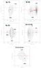 |
Fig. D.1 [O i]6300 Å continuum subtracted position velocity (PV) diagrams of five sources exhibiting strong HVC. The straight line indicates the position of the continuum while red dots highlight the peaks of the blue- and red-shifted HVC (i.e. HVB and HVR, respectively) and of the LVC. The HVC peaks are systematically shifted with respect to the continuum position, showing that this component is extended. |
All Tables
All Figures
|
Fig. 1 Examples of [O i]6300 Å spectra of sources with and without a HVC. Blue-dashed lines indicate the Gaussian profiles used to fit the different components, and the red-dashed line is the final best fit. |
| In the text | |
|
Fig. 2 Distribution of accretion (top) and stellar (bottom) luminosity for all the sources of our sample is depicted in black. Red and blue histograms are relative to sources where the HVC has been detected and not-detected respectively. In the upper corner of each plot the percentage of HVC detection in two ranges of luminosities is indicated. |
| In the text | |
|
Fig. 3 Ratio between the HVC and LVC [O i]6300 Å line luminosities as a function of the accretion luminosity. Black, red and green symbols indicate sources in Lupus, Chamaeleon and σ Orionis clouds, respectively. Arrows refer to 3σ upper limits for the HVC luminosity. |
| In the text | |
|
Fig. 4 [O i]6300 Å line luminosity of the LVC is plotted as a function of, from top to bottom, stellar mass, stellar luminosity and accretion luminosity. Colour codes for the symbols are as in Fig. 3. Arrows refer to 3σ upper limits. The dashed line indicates the linear regression whose parameters are given in the upper right corner of each figure, together with the correlation parameter. |
| In the text | |
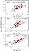 |
Fig. 5 Same as Fig. 4 but for the [O i]6300 Å luminosity in the HVC. |
| In the text | |
|
Fig. 6 [O i]6300 Å line luminosity of the LVC (bottom) and HVC (top) is plotted as a function of the mass accretion rate. Symbols and labels are as in Fig. 4. |
| In the text | |
|
Fig. 7 Correlations between the [O i]6300 Å line and accretion luminosities, both normalized by the stellar luminosity. Symbols and labels are as in Fig. 4. |
| In the text | |
|
Fig. 8 Accretion luminosity derived by modelling the UV excess is compared with that estimated through the L[O i] LVC vs. Lacc relationships for the sub-luminous sources. |
| In the text | |
|
Fig. 9 Mass accretion (Ṁacc) vs. mass ejection (Ṁjet) rates. The mass ejection has been measured from the [O i]6300 Å luminosity assuming a jet tangential velocity of 100 km s-1 and gas temperature and density of 10 000 K and 5 × 104 cm-3 respectively. Black, red and green symbols are as in Fig. 4, while blue triangles indicate the values for the sample of Taurus sources of H95. Updated mass accretion rates from these sources are estimated from the data in Rigliaco et al. (2013). Average data point uncertainty is indicated with a cross on the left side of the plot. Arrows refer to upper limits on Ṁjet derived from the 3σ upper limits on the L[O i] HVC luminosity. |
| In the text | |
|
Fig. 10 Distribution of ejection efficiency (Ṁjet/Ṁacc) for the global sample. Black histogram are values for sources with detected HVC while red dotted histogram indicates the distribution of upper limits. |
| In the text | |
|
Fig. 11 Upper panel: log of the Ṁjet/Ṁacc ratio plotted as a function of the log of the stellar mass. The three horizontal dashed lines correspond to Ṁjet/Ṁacc = 1, 0.1 and 0.01. Black, red and green symbols are as in Fig. 4 while blue triangles refer to the sources in Taurus (see caption of Fig. 9). Lower panel: log of the Ṁjet/Ṁacc ratio plotted as a function of the log of the mass accretion rates. |
| In the text | |
|
Fig. 12 Absolute value of the peak velocity in the HVC (Vpeak(HVC)) is plotted as a function of the disc inclination angle for a sub-sample of sources in Lupus where idisc has been measured from ALMA observations (Tazzari et al. 2017). Upper limits refer to sources with measured inclination angles that don’t have a HVC component. An upper limit of Vpeak(HVC) of 40 km s-1 has been considered in the plot for these sources. |
| In the text | |
|
Fig. 13 Correlation between Vpeak(HVC) and the deconvolved line width of the LVC. The vertical dashed line at ΔV(LVC) = 40 km s-1 separate sources where the LVC is dominated by a narrow component (NC) or a broad component (BC) according to Simon et al. (2016). Symbols are as in Fig. 4. |
| In the text | |
|
Fig. D.1 [O i]6300 Å continuum subtracted position velocity (PV) diagrams of five sources exhibiting strong HVC. The straight line indicates the position of the continuum while red dots highlight the peaks of the blue- and red-shifted HVC (i.e. HVB and HVR, respectively) and of the LVC. The HVC peaks are systematically shifted with respect to the continuum position, showing that this component is extended. |
| In the text | |
Current usage metrics show cumulative count of Article Views (full-text article views including HTML views, PDF and ePub downloads, according to the available data) and Abstracts Views on Vision4Press platform.
Data correspond to usage on the plateform after 2015. The current usage metrics is available 48-96 hours after online publication and is updated daily on week days.
Initial download of the metrics may take a while.