| Issue |
A&A
Volume 606, October 2017
|
|
|---|---|---|
| Article Number | A142 | |
| Number of page(s) | 12 | |
| Section | Interstellar and circumstellar matter | |
| DOI | https://doi.org/10.1051/0004-6361/201630265 | |
| Published online | 26 October 2017 | |
Search for grain growth toward the center of L1544 ⋆,⋆⋆
1 Max-Planck-Institüt für extraterrestrische Physik, Giessenbachstrasse 1, 85748 Garching, Germany
e-mail: achacon@mpe.mpg.de
2 Department of Physics, PO Box 64, 00014 University of Helsinki, Finland
3 Kapteyn Astronomical Institute, University of Groningen, PO Box 800, 9700 AV Groningen, The Netherlands
4 Univ. Grenoble Alpes, CNRS, IPAG, 37000 Grenoble, France
Received: 16 December 2016
Accepted: 29 June 2017
In dense and cold molecular clouds dust grains are surrounded by thick icy mantles. It is not clear, however, if dust growth and coagulation take place before the protostar switches on. This is an important issue as the presence of large grains may affect the chemical structure of dense cloud cores, including the dynamically important ionization fraction and the future evolution of solids in protoplanetary disks. To study this further, we focus on L1544 – one of the most centrally concentrated pre-stellar cores on the verge of star formation – which has a well-known physical structure. We observed L1544 at 1.2 and 2 mm using NIKA, a new receiver at the IRAM 30 m telescope, and we used data from the Herschel Space Observatory archive. We find no evidence of grain growth toward the center of L1544 at the available angular resolution. Therefore, we conclude that single-dish observations do not allow us to investigate grain growth toward the pre-stellar core L1544 and high-sensitivity interferometer observations are needed. We predict that dust grains can grow to 200 μm in size toward the central ~300 au of L1544. This implies a dust opacity change of a factor of ~2.5 at 1.2 mm, which can be detected using the Atacama Large Millimeter and submillimeter Array (ALMA) at different wavelengths and with an angular resolution of 2′′.
Key words: ISM: clouds / ISM: individual objects: L1544 / dust, extinction / opacity / stars: formation
Based on observations carried out with the IRAM 30 m telescope. IRAM is supported by INSU/CNRS (France), MPG (Germany), and IGN (Spain).
The FITS files of the maps presented here are only available at the CDS via anonymous ftp to cdsarc.u-strasbg.fr (130.79.128.5) or via http://cdsarc.u-strasbg.fr/viz-bin/qcat?J/A+A/606/A142
© ESO, 2017
1. Introduction
Pre-stellar cores are self-gravitating starless dense cores with clear signs of contraction motions and chemical evolution (Crapsi et al. 2005). They are formed within molecular clouds, due to the influence of gravity, magnetic fields, and turbulence. They are thought to be on the verge of star formation, and therefore represent the initial conditions in the process of star formation (Bergin & Tafalla 2007; Caselli & Ceccarelli 2012). These systems are characterized by high densities (nH2> 105 cm-3) and low temperatures (T< 10 K) toward their central regions (Crapsi et al. 2007).
In dense and cold molecular clouds dust grains are surrounded by thick icy mantles (e.g., Boogert et al. 2015, and references therein). It is not clear, however, if dust growth and coagulation take place before a protostar is born. This is an important issue as dust coagulation may affect the formation and evolution of protoplanetary disks forming from molecular clouds (Zhao et al. 2016). Foster et al. (2013) find a strong correlation between the visual extinction and the slope of the extinction law toward the Perseus molecular cloud. This can be interpreted as grain growth, but it is not clear if grain coagulation is needed or if the growth of icy mantle can explain the observed correlation. Large grains are also detected in young protoplanetary disks, again suggesting that grain growth may already be at work in the earlier dense core phases (Testi et al. 2014). There is evidence of large (micrometer-sized) grains through the observed extended emission at 3.6 μm in dense cloud cores (known as the coreshine effect; Pagani et al. 2010), but this interpretation has been questioned by Jones et al. (2013), who suggested that amorphous hydrocarbon material could actually produce the observed coreshine without the need of large grains. Moreover, Andersen et al. (2014) found a similar threshold for the coreshine and water ice, with the scattering efficiency at 3.6 μm increasing with the increase in the water-ice abundance, suggesting that water ice mantle growth in dense clouds may be at least partially responsible for the coreshine effect. However, recent findings by Lefèvre et al. (2016) show that the mid-infrared scattering phenomenon is still present at 8 μm and that grains proposed in Foster et al. (2013) would fail to explain scattering at such a long wavelength, as would the uncoagulated ice covered grains advocated by Andersen et al. (2014).
The study of the dust emission at long wavelengths sensitive to the larger grains is therefore important in order to gain a better understanding of the grain size distribution in the early phases of star formation. This emission depends on dust grain properties such as structure, size, and composition. Here we focus on the dust opacity and the spectral index, two parameters that depend directly on the grain size distribution.
The opacity, κν, is a measurement of the dust absorption cross sections weighted by the mass of the gas and dust. As explained by Kruegel & Siebenmorgen (1994), when dust grains are small compared to the wavelength (the so-called Rayleigh limit), the mass absorption coefficient does not depend on the grain size, but only on the mass; when the grain size is much larger than the wavelength, the absorption coefficient depends inversely on the grain size; and when a ~ λ (a being the grain radius), the mass absorption coefficient can increase up to 10 times its value because at these wavelengths dust grains are better radiators (Kruegel & Siebenmorgen 1994). When dust grains are coated by ices, their cross section increases and, consequently, so does κν. This same trend is seen with fluffy dust grains (Kruegel & Siebenmorgen 1994; Ossenkopf & Henning 1994). Therefore, variations in the value of κν along the spectrum can be a strong indicator of grain growth.
The dust opacity can be approximated by a power law at millimeter wavelengths, κν ~ νβ, where β is the emissivity spectral index (Hildebrand 1983). For β, a more complex analysis is needed. Typical values found in the interstellar medium (ISM) at far-infrared and submillimeter wavelengths lie in the range 1.5–2. In presence of large grains, which increase the dust opacity at longer wavelengths, β can decrease to values close to or below 1 (Ossenkopf & Henning 1994; Draine 2006). When the minimum size of the distribution is lower than 1 μm, β is only affected by the largest grains and not by the smaller grains (Miyake & Nakagawa 1993; Draine 2006).
Laboratory measurements of the opacity and the spectral index at millimeter wavelengths found a dependence of the mass absorption on temperature for different grain compositions (Agladze et al. 1996; Mennella et al. 1998; Boudet et al. 2005; Coupeaud et al. 2011; Demyk et al. 2013). Agladze et al. (1996) found two different behaviors depending on the temperature range: for very low temperatures (1.2–20 K) the millimeter opacity decreases with increasing temperature, while for temperatures between 20 and 30 K it increases or is constant with temperature. This trend is the opposite for β. However, at mm-wavelengths the measured changes are not significant (within 20%) when the temperature is varied between 6 and 10 K, which is the temperature range relevant to the central regions of pre-stellar cores. Boudet et al. (2005) and Coupeaud et al. (2011) found similar results for amorphous material, as they observed an increase in the spectral index (decrease in the opacity) while decreasing the temperature (for T> 10 K). However, when they let the material crystallize, no temperature dependence was detected. Additionally, they also reported a frequency dependence on the opacity and the spectral index. Another interesting result was found by Demyk et al. (2013), who showed two extreme and completely different results depending on the material analyzed for temperatures ranging from 10 K to 300 K. For wavelengths longer than 500 μm, the spectral index value could take values higher than 2.5 and lower than 1.5 depending on the composition of the sample, which in their case depends on the oxidation state of the iron. This means that the increase in the opacity in the studied temperature range is more important at longer wavelengths. What Demyk et al. (2013) conclude is that the emission from dust cannot be described by only one power-law spectrum, but should be characterized by different spectral indexes at different wavelengths.
There are several astronomical studies constraining the value of β in protoplanetary disks, where it is known that dust coagulation takes place, giving birth to future planets. Natta & Testi (2004) found that despite the composition dependence and grain distribution shape, dust grains of 1 mm in size lead to β values lower than 1. For earlier stages in the process of star formation, Schnee et al. (2014) found low values for the spectral index toward OMC 2/3 with a low anticorrelation between β and temperature, which may indicate the presence of grains from millimeter size up to centimeter size. However, this was subject of further study by Sadavoy et al. (2016), who found higher values of the spectral index and suggested that the observations from Schnee et al. (2014) were contaminated or deviated from a single power law. After studying extinction maps, Forbrich et al. (2015) found that while a single spectral index can reproduce their observational data, the opacity increases toward the center of the starless core FeSt 1-457, possibly indicating grain growth. At larger scales, using Planck and Herschel results, Juvela et al. (2015a,b) observed that the opacity increases with density and that there is an anticorrelation between the spectral index and the temperature.
Obtaining a value of the spectral index at early stages of star formation is a difficult task due to the known degeneracy between the spectral index and temperature, which appears when the spectral energy distribution of the dust emission is fitted using a least-squares method to obtain the temperature, density, opacity, and spectral index of the observed object (Shetty et al. 2009a,b). Moreover, it has also been proved that uncertainties in the measured fluxes, and an incorrect assumption of isothermality and the noise itself, can mimic the observed anticorrelation between the temperature and the spectral index of the dust (Shetty et al. 2009a,b).
Therefore, taking into account these studies and previous results on the spectral index, it is not clear what to expect from observations toward the dense and cold pre-stellar cores. Nevertheless, any variation in the κν and/or β across a cloud core, from the outskirts to the center, would indicate grain growth. Köhler et al. (2015) show that dust evolution in dense clouds produces significant variations (factors of a few) in the opacity, while the spectral index changes by less than 30%, so that κν variations should be easier to measure. Moreover, if the physical structure of the cloud is known, it is possible to directly measure the variation in the opacity across a core at millimeter wavelengths, while for the spectral index a multiwavelength study is needed.
In this work we focus on L1544, a well-known pre-stellar core in the Taurus Molecular Cloud at a distance of 140 pc. The zone within the central 1000 au is still unexplored, but we know that the temperature drops down to 7 K toward the central 2000 au (Crapsi et al. 2007) and it shows clear signs of contraction (Caselli et al. 2012). Detailed modeling of L1544 (Keto & Caselli 2010) found that an increase in the dust opacity is needed to reproduce the drop in the measured temperature toward the central 2000 au. This could be an indication of fluffy grains in the core center (Ossenkopf & Henning 1994; Ormel et al. 2009) where CO is heavily frozen (Caselli et al. 1999) and volume densities become larger than 106 cm-3. The presence of fluffy grains can only be verified by multiwavelength millimeter observations. The well-known physical structure of L1544, with its high volume densities and centrally concentrated structure, makes this object the ideal target to study possible variation in the opacity. For this, we used the continuum emission at 1.2 mm and 2 mm from the IRAM 30 m telescope with an angular resolution of 12.5′′ and 18.5′′, respectively (at 140 pc, this corresponds to 1800 and 2600 au). This is the first study of opacity variation and grain growth across a pre-stellar core at this resolution and at such long wavelengths using a single-dish telescope.
The paper is organized as follows. In Sect. 2 we describe the millimeter data for L1544 obtained with NIKA and far-IR data obtained with SPIRE. In Sect. 3 we describe the results for the maps of the spectral index and the opacity assuming constant temperature and density across the cloud, as done in previous studies. This is compared later with the same results assuming variations on both the temperature and the density along the line of sight, making use of the profiles presented by Keto et al. (2015). We end this section by presenting the results for the opacity and spectral index from the combination of NIKA and Herschel/SPIRE data, and a comparison between the modeled emission and the observations. In Sect. 4 we compare our observational findings with a simple grain growth evolution model. In Sect. 5 we summarize our findings.
2. Observations
2.1. NIKA
The observations were carried out using the IRAM 30 m telescope located at Pico Veleta (Spain) during the spring of 2014 using the New IRAM KID Array (NIKA; Catalano et al. 2014; Calvo et al. 2013). The project number is 151-13. A region of 3′ × 3′ was mapped using the Lissajous pattern to observe the pre-stellar core L1544, α(J2000) = 05h04m17.21s and δ(J2000)=+25°10′42.8′′ (dust peak from Ward-Thompson et al. 1999), at 1.2 and 2 mm. The main beam widths are 12.5′′ at 1.2 mm and 18.5′′ at 2 mm. At a distance of 140 pc, this corresponds to a resolution of 1800 au and 2600 au, respectively. The KID array has a field of view of 1.8′ at 1.2 mm and 2.0′ at 2 mm.
The data were reduced by the NIKA team. The original maps were corrected by the ratio of main beam to full beam, which is 1.56 at 1.2 mm and 1.35 at 2 mm, with an uncertainty of ~10% on these factors. The noise level of the map at 1.2 mm is 0.007 Jy/12.5′′-beam and that of the map at 2 mm is 0.002 Jy/18.5′′-beam. In Fig. 1, both images have been converted into MJy/sr. In Sects. 3.2.1 and 3.2.2, the two maps have been convolved to a common resolution of 19′′, reducing the noise levels to 0.9 and 0.15 MJy/sr at 1.2 and 2 mm, respectively. The absolute uncertainty on the surface brightness is ~15%.
The maps show two lobes of negative surface brightness: one to the northeast and another to the southwest, due to filtering of extended emission. As the field of view of the camera differs by ~10% between the two NIKA bands, we expect this filtering to be the same for both bands, and therefore it should not affect our analysis where both bands are treated simultaneously (see Sect. 3.2). To quantify this statement, a study of the power spectra of the two bands is performed in Appendix A. Moreover, Adam et al. (2015) used simulations to estimate at which spatial scales NIKA filters the emission. They found that NIKA filtering starts to be important on scales larger than the field of view and that it is the same for the two bands. This is also mentioned in Adam et al. (2017). Thus, here filtering effects are also assumed to be within the errors found in Sect. 3.3 where the results are shown for each band separately, and only for the region above 3σ detection, which is ~1′ in size, and therefore smaller than the field of view.
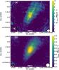 |
Fig. 1 Maps of the continuum emission of L1544 at a) 1.2 mm and b) 2 mm. The angular resolution is 12.5′′ at 1.2 mm and 18.5′′ at 2 mm (HPBW shown by the white circle in the bottom right corner) and the contours are indicating the different σ levels of the emission above 3σ (3σ, 4σ, 5σ, etc., where σ1.2 mm = 1.4 MJy/sr and σ2 mm = 0.15 MJy/sr). |
2.2. Herschel
The Herschel/SPIRE data at 250, 350, and 500 μm used here have already been presented by Spezzano et al. (2016). They are part of the Level 3 mosaic maps of the Taurus molecular cloud complex observed in the SPIRE/PACS parallel mode in the course of the Herschel Gould Belt Survey (André et al. 2010). The data downloaded from the Herschel Science Archive (HSA) are reduced using the Standard Product Generation (SPG) software version 14.2.1. These data are calibrated assuming that the source is infinitely extended, and the surface brightness zero points have been corrected using absolute levels from Planck maps. The SPIRE flux densities are assumed to be accurate to 10% (Bertincourt et al. 2016). The resolution of Herschel at 500 μm is ~38.5′′. When combining the SPIRE maps with the NIKA data, we took into account that SPIRE is sensitive to the extended emission, while NIKA filters it out. To compensate for this difference, we subtracted from each SPIRE map a value that corresponds to the average surface brightness just outside the region seen by NIKA. The region where these averages are calculated was determined from the NIKA 1.2 mm map; this is a ~35 arcsec wide ring outside the 1σ contour. After this subtraction, the peak emission and the errors at 250, 350, and 500 μm are 153 ± 12, 120 ± 12 and 62 ± 9 MJy/sr, respectively. The dependence of our results on the width of the ring was checked, and found not significant.
3. Dust properties
3.1. Theoretical background
Dust grains emit as modified blackbodies:  (1)where Bν(Td) is the blackbody function at a temperature Td:
 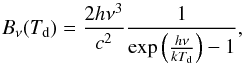 (2)Sν is the flux density, Ω is the solid angle subtended by the beam, κν is the dust opacity at frequency ν (the absorption cross-section for radiation per unit mass of gas), μH2 = 2.8 is the molecular weight per hydrogen molecule (Kauffmann et al. 2008), mH is the mass of the hydrogen atom, and NH2 is the molecular hydrogen column density. The dust opacity can be approximated by a power law at mm wavelengths (Hildebrand 1983)
 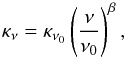 (3)where κν0 is the opacity at a reference frequency ν0 and β is the spectral index. We assume a dust-to-gas ratio of 0.011 in Eq. (1), where there are several unknown parameters: the density, the temperature, the opacity, and the spectral index.
The above equations are typically used to derive dust temperatures, densities, and masses, assuming isothermal clouds and using fixed values for the dust opacity and the spectral index (e.g., Schnee & Goodman 2005). The value of the dust opacity is normally taken from Table 1 of Ossenkopf & Henning (1994), and the spectral index is mostly assumed to be within the range of 1.5–2 for pre-stellar cores. However, these approximations and assumptions can give incorrect temperatures, densities, and masses, or false anticorrelations between β and the dust temperature (Shetty et al. 2009a,b).
Here we first follow the calculation of the spectral index done by Schnee & Goodman (2005) assuming a constant temperature of 10 K for the core. We then do the same calculation but using the temperature and density profiles derived by Keto et al. (2015) and compare them to the constant temperature case. Finally, we consider a constant value of the spectral index and the opacity across the core to see if the observed millimeter emission can be reproduced by modeling.
3.2. Spectral index and opacity of the dust using NIKA
3.2.1. Assuming constant temperature
For isothermal clouds, the spectral index value can be derived using the ratio of the surface brightnesses at 1.2 and 2 mm: 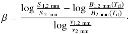 (4)Considering a constant κ250 μm = 0.1 cm2 g-1 value (Hildebrand 1983), we can also derive a map for the opacity at 1.2 mm:
  (5)The values have only been derived for surface brightnesses above the 3σ level of the maps at 1.2 and 2 mm.
The resulting β and κ1.2 mm maps are shown in Fig. 2. There is a slight decrease in the spectral index toward the central regions, although its value (~2) is still consistent with interstellar medium (ISM) dust not affected by coagulation. This observed spatial gradient, which shows appreciable variations of ~30% with an errorbar of ~25% in the spectral index value, reflects the variation in the S1.2 mm/S2 mm ratio across the core as the other quantities in Eq. (4)are constant. Therefore, an increase in the temperature in the outskirts would necessarily mimic an increase in β.
The opacity shows a significant increase (a factor of 10) toward the center, with errorbars of ~0.001 cm2 g-1 in the determination of the opacity values. This could indicate grain growth. However, this result is also affected by the underlying assumption that the temperature is constant across the core, while this is not the case for L1544 (see Sect. 3.2.2). Moreover, κ250 μm may vary as well across the cloud, so the assumption of a constant κ250 μm along the line of sight may not be a good one.
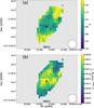 |
Fig. 2 Maps of the a) spectral index and b) opacity at 1.2 mm assuming a constant core temperature of 10 K and a constant κ250 μm = 0.1 cm2 g-1 value (Hildebrand 1983). The 1.2 mm map was convolved to the 2 mm band resolution, which is 19′′ (HPBW shown by the white circle in the bottom right corner). In both cases, the crosses mark the peak of the emission corresponding to the final 1.2 mm map convolved to 19′′. |
3.2.2. Using the known dust temperature and density profiles of L1544
For L1544 we can make use of the radial density profile, nH2(r), and temperature profile, T(r), derived by Keto et al. (2015). These profiles correspond to a spherical model that follows the evolution of an unstable Bonnor-Ebert sphere, reproducing previous observations of L1544. The volume density, nH2, is related to the column density, NH2, as  , i.e., the column density is the volume density integrated over the line of sight; T(r) and nH2(r) are shown in Fig. 3.
The knowledge of the temperature and density of the core leaves Eq. (1)with only two unknown parameters: the dust opacity and spectral index. Therefore, taking into account the variation in the density and the temperature along the line of sight, and the units we use (MJy/sr), Eq. (1)for each pixel transforms to ![\begin{equation} S_{\nu}(r_{ij}) = \kappa_{\nu}(r_{ij}) \mu_{\rm H_2} m_{\rm H} \int_{s_{\rm los}}^{}{B_{\nu}[T_{\rm d}(r_{ij})]n_{\rm H_{2}}(r_{ij}) {\rm d}s}, \label{eqSS} \end{equation}](/articles/aa/full_html/2017/10/aa30265-16/aa30265-16-eq53.png) (6)where s is the path along the line of sight, which has a direct relation with the radius r, and i and j represent the pixel coordinates on the map.
(6)where s is the path along the line of sight, which has a direct relation with the radius r, and i and j represent the pixel coordinates on the map.
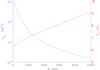 |
Fig. 3 Temperature (red) and density (blue) profiles of L1544 from Keto et al. (2015). |
As in the previous section, the ratio between the surface brightnesses at 1.2 and 2 mm gives us an estimate of β, and consequently the value of κν, although in this case we derive it using ![\begin{equation} \kappa_{\nu}(r_{ij}) = \frac{S_{\nu}(r_{ij})}{ \mu_{\rm H_2} m_{\rm H} \int_{s_{\rm los}}^{}{B_{\nu}[T_{\rm d}(r_{ij})]n_{{\rm H}_{2}(r_{ij})} {\rm d}s} }\cdot \label{opacity_eq} \end{equation}](/articles/aa/full_html/2017/10/aa30265-16/aa30265-16-eq58.png) (7)This approach is more accurate than the method used in Sect. 3.2.1 because it does not assume a constant value for the opacity at a reference frequency, but it uses the clear incorrect assumption that the spectral index and the opacity do not change along the line of sight. This may not be the case: if changes from the outskirts to the center of the core are present, the same change should apply along the line of sight toward the center. This approach also assumes that the spectral index does not depend on the temperature, but as we see in Sect. 1, no significant temperature dependence is expected within the temperature range relevant for L1544 (e.g., Agladze et al. 1996; Mennella et al. 1998; Boudet et al. 2005; Coupeaud et al. 2011; Demyk et al. 2013).
(7)This approach is more accurate than the method used in Sect. 3.2.1 because it does not assume a constant value for the opacity at a reference frequency, but it uses the clear incorrect assumption that the spectral index and the opacity do not change along the line of sight. This may not be the case: if changes from the outskirts to the center of the core are present, the same change should apply along the line of sight toward the center. This approach also assumes that the spectral index does not depend on the temperature, but as we see in Sect. 1, no significant temperature dependence is expected within the temperature range relevant for L1544 (e.g., Agladze et al. 1996; Mennella et al. 1998; Boudet et al. 2005; Coupeaud et al. 2011; Demyk et al. 2013).
The β and κ1.2 mm maps are shown in Fig. 4. The behavior of the spectral index does not seem to differ much from that presented in Sect. 3.2.1 where a constant temperature was assumed. However, the spatial variations are not significant here; they are negligible within the errors (~25%). This is due to the fact that the ratio of the term ![\hbox{$\int_{s_{\rm los}}^{}{B_{\nu}[T_{\rm d}(r_{ij})]n_{\rm H_{2}}(r) {\rm d}s}$}](/articles/aa/full_html/2017/10/aa30265-16/aa30265-16-eq59.png) at the two different frequencies does not differ significantly from the value computed assuming a constant temperature of 10 K. On the other hand, the opacity value changes significantly (~60% with uncertainties of 20%). Thus, the overall κ1.2 mm value dispersion is two times larger than before, and surprisingly, the opacity now shows a decreasing trend toward the central regions, contrary to the expectation of grain growth.
at the two different frequencies does not differ significantly from the value computed assuming a constant temperature of 10 K. On the other hand, the opacity value changes significantly (~60% with uncertainties of 20%). Thus, the overall κ1.2 mm value dispersion is two times larger than before, and surprisingly, the opacity now shows a decreasing trend toward the central regions, contrary to the expectation of grain growth.
The simplest explanation of this apparently contradictory result is that the model assumes spherical symmetry, while L1544 is clearly an elongated core, with an aspect ratio of about 2. This implies that the model cannot be used for the outer parts of the cloud, in particular along the major axis. Moreover, the derivation of the spectral index using the method of the flux ratios with only two wavelengths in the Rayleigh-Jeans limit leads to inaccurate values due to the uncertainties on the fluxes (Shetty et al. 2009b).
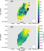 |
Fig. 4 Maps of the a) spectral index and b) opacity at 1.2 mm derived with the method described in Sect. 3.2.2. The angular resolution is 19′′ (HPBW shown by the white circle in the bottom right corner). The crosses mark the peak of the emission corresponding to the final 1.2 mm map convolved to 19′′. |
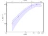 |
Fig. 5 Fit of the SED to the five spectral windows available at 250, 350, 500, 1250, and 2000 μm at the peak emission when convolving and regridding all windows to the resolution of the 500 μm band. The error bars indicate the weights used in the fitting, which correspond to the uncertainties and noise associated with the data. The shadowed blue region show the 95% confidence intervals of the fitted parameters. |
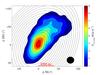 |
Fig. 6 Ellipses where the emission has been averaged for the 1.2 mm and 2 mm maps superimposed on the 1.2 mm continuum map of L1544. Only the colored region is included in the average. The resolution is 19′′ (HPBW shown by the black circle in the bottom right corner). For Herschel/SPIRE the distance between concentric ellipses is larger, due to a larger pixel size and resolution. For both NIKA and SPIRE, the distance between ellipses is chosen to be ~1.8 pixels, averaging in a 1 pixel wide ring. |
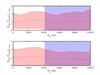 |
Fig. 7 Ratio between the observed and the modeled surface brightnesses at 1.2 mm (top) and 2 mm (bottom) as a function of geometric mean radius of the ellipses in Fig. 6, using the temperature and density profiles from Keto et al. (2015) and an opacity value of κ250 μm = 0.2 ± 0.1 cm2 g-1 and β = 2.3 ± 0.4. The shadowed red region represents the uncertainties on the fluxes, the opacity, and the spectral index. The shaded blue region indicates the zone where the observed surface brightness is below 3σ. |
3.3. Spectral index and opacity of the dust using NIKA and SPIRE
Because of the complex and unknown dependence of the spectral index on the temperature, the uncertainties on the surface brightnesses, and the spherically symmetric model, we consider a different approach here. The modeled densities and temperature profiles are now used to predict the emission at 1.2 and 2 mm, fixing the values of the opacity and the spectral index of the dust. The adopted values for the opacity and the spectral index are derived from the best least-squares fit to the surface brightnesses in the five spectral windows available (three from Herschel/SPIRE and two from NIKA) toward the peak emission of L1544 at each band. We assume that the opacity and the spectral index are independent because possible degeneracies between the two parameters are beyond the scope of this paper and are not well-known. Before fitting, the five maps were convolved and regridded to the lowest resolution, i.e., the 500 μm band (~38.5′′ beam and 14′′ pixel size), and the Herschel/SPIRE bands have been color-corrected assuming an extended source with a spectral index of 2.0. From the model, we derive the term for each pixel in the maps at each frequency and smooth this to the common resolution to introduce in the fitting the corresponding terms, which depend on temperature and density in the center. A least-squares fit is performed to find which values of the opacity and spectral index best match the observations. This procedure is iterative: the spectral index and the corresponding color-correction of the SPIRE bands are varied until a convergence is found. The resultant spectral energy distribution (SED) is shown in Fig. 5. The values of κ250 μm and β found with this procedure are  where the errors indicate the 95% confidence intervals of the estimates of the fit. Within the uncertainties, this value for the opacity is in agreement with those calculated by Ossenkopf & Henning (1994) for thin and thick ice mantles. However, the spectral index is significantly larger than the value derived by Planck for L1544: 1.608 ± 0.007 (Planck Collaboration X 2016). This difference could be due to the significantly larger beam for the high-resolution (7.5 arcmin) thermal dust emission map derived using Planck frequencies above 143 GHz. In the derivation of the spectral index from Planck, a constant dust temperature of 16.55 ± 0.08 K in a region of 1° × 1° in size is assumed. This temperature is higher than that observed with ammonia by Crapsi et al. (2007). The sensitivity of Planck to large emission and its resolution imply that the variations in the temperature are averaged over a bigger structure along the line of sight, dominated by the envelope, increasing the observed temperature and tracing better the outer part of the core. Moreover, if no temperature variation along the line of sight is taken into account, β is expected to be underestimated (Juvela et al. 2015a); therefore, we adopt our derived value of β as representative for L1544.
To make the comparison between the modeled emission, which is for a sphere, and the observations, we average the emission of the core in ellipses at different distances from the center with an inclination of ~65° (see Fig. 6). Only emission within the colored map in Fig. 6, which corresponds to positive surface brightnesses, is considered. The results are shown in Fig. 7 for NIKA and in Fig. 8 for SPIRE, where the ratio between the observed and modeled surface brightnesses is reported as a function of radius. For the observed emission this radius corresponds to the geometric mean of the major and minor axes of the ellipses. The resolution is the native resolution of each band, which corresponds to 18.5′′, 12.5′′, 38.5′′, 26.8′′, and 20.3′′ at 2 mm, 1.2 mm, 500 μm, 350 μm, and 250 μm, respectively. The agreement is within a factor of 2 in all bands, which leads to the conclusion that there is no need to modify the opacity or the spectral index toward the central regions to reproduce the observed surface brightnesses. We have also checked the dependence of this ratio with the value of the spectral index and the opacity: the mm wavelengths are sensitive to the variation of β and κ250 μm, increasing and decreasing the surface brightness by a factor of 2 or more. However, if the spectral index and the opacity increase at the same time within the 95% confidence intervals, the ratio between the observed and the estimated surface brightness remains constant around 1 within the errors. This occurs because an increase in the spectral index decreases the expected surface brightness at mm wavelengths, but an increase in the opacity can compensate this effect and increases the prediction by the same amount. Therefore, variations in these two parameters within the uncertainties (50% and 20% for the opacity and the spectral index, respectively) cannot be detected with our data. The decrease in the ratio between the observed and modeled surface brightness at the outskirts of the core in the case of SPIRE is due to the harsh filtering applied to the data, and the error associated with this procedure is large at Rm> 4000 au because the filtering relies on the shape of the 1.2 mm emission, which goes below the 3σ level at Rm> 4000 au (see Sect. 2.2 and Appendix A).
These results indicate that the emission is consistent with a constant opacity, at the resolution and sensitivity achieved with NIKA. This is in apparent contradiction with the results of Keto & Caselli (2010), who needed to increase the opacity toward the central regions to reproduce the drop in the temperature measured by Crapsi et al. (2007) using interferometric observations. As explained in Sect. 4.3, higher angular resolution observations are needed to test the prediction made by Keto & Caselli (2010).
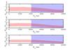 |
Fig. 8 Ratio between the observed and the modeled surface brightnesses at 500 μm (top), 350 μm (middle), and 250 μm (bottom) as a function of the geometric mean radius of the ellipses, as explained in Fig. 6, using the temperature and density profiles from Keto et al. (2015) and an opacity value of κ250 μm = 0.2 ± 0.1 cm2 g-1 and β = 2.3 ± 0.4. The shadowed red region represents the uncertainties on the fluxes, the opacity, and the spectral index. The shaded blue region indicates the zone where the millimeter observed surface brightness is below 3σ as the artificial filtering of Herschel/SPIRE relies on the shape of the 1.2 mm emission (see Sect. 2.2 and Appendix A). |
4. Model predictions on grain growth and comparison with our data
The theoretical studies on grain evolution of Ormel et al. (2009, 2011) show that little grain growth takes place when the cloud lifetime is similar to the free-fall time because the process of coagulation takes longer. However, pre-stellar cores may span a range of lifetimes which significantly exceed the free-fall time (see, e.g., Brünken et al. 2014; Kong et al. 2015; Könyves et al. 2015). If there are processes sustaining the cloud against gravitational collapse (e.g., turbulence and/or magnetic fields), some dust coagulation could take place. Ormel et al. (2009, 2011) show that about 100 μm dust grains can form if gas densities of 105 cm-3 can be maintained for 10 Myr, while after 1 Myr dust grains can grow up to ~4 μm.
In the following, we present an analytical solution (Blum 2004) to estimate grain growth. Ormel et al. (2009) compared this analytical solution with their Monte Carlo simulation, finding a very good match. We apply this model to the pre-stellar core L1544. As mentioned, L1544 is a very well-known pre-stellar core, centrally concentrated and with high central densities (~106 cm-3 within a radius of 500 au, see Fig. 3) which makes it unique and ideal for this study. We consider two different cases: a static core with the physical structure given in Fig. 3, and a dynamical core based on the quasi-equilibrium contraction model of Keto et al. (2015), which best reproduce spectroscopic data.
4.1. Analytical model
We used a simple analytical model derived by Blum (2004), and checked by Ormel et al. (2009), who compared it with their Monte Carlo simulation and demonstrated its validity for average molecular cloud conditions (density 105 cm-3, temperature 10 K, and intermediate velocity regimes2, Ossenkopf 1993; Ormel et al. 2009; Ormel & Cuzzi 2007). The analytical model is based on the assumption of a monodisperse distribution of spherical particles. As the particles coagulate, they form bigger grains made out of N monomers with a characteristic filling factor that describes their shape (fractal or compact). Here we use the terminology used by Ormel et al. (2009), as well as the parameters and equations derived from their simulations.
The initial evolution of the process of grain growth through grain-grain collisions can be divided into two different regimes: the fractal regime and the compaction regime (Ormel et al. 2009; Blum 2004). The fractal regime is characterized by growth with no visible restructuring of the grain; which also includes the hit-and-stick regime. By contrast, during the compaction regime dust grains undergo changes in their structure. The transition point from one regime to another is determined by the parameter N1 (see Appendix A from Ormel et al. 2009), which strongly depends on the grain size. The bigger the grain, the lower N1 and the easier it is to reach the compact limit. Instead, N2 (see Appendix A in Ormel et al. 2009) defines the transition point between the compaction regime and the fragmentation regime where grains start to lose monomers in grain-grain collision. When this regime is reached, it is assumed that the grains do not grow further, and the growth is compensated with fragmentation. When grains are close to this regime in high-density environments, the simple model overestimates the growth compared to Ormel et al. (2009), due to the high dependency of N1 with density.
To define the transition points N1 and N2, we apply the same criteria as in Ormel et al. (2009). The complete expressions for N1 and N2 can be found in their Appendix A and follow 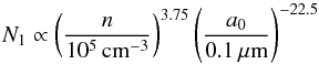 (8)and
 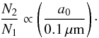 (9)It should be noted here that n is the number density of gas molecules, related to nH2 as n ≃ nH/ 1.7 = 2nH2/ 1.7, and a0 is the initial grain size.
As derived in Blum (2004) and used by Ormel et al. (2009), the equation to solve is 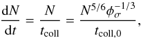 (10)where N is the number of monomers and φσ is the filling factor of the dust grain, a quantity that indicates the fluffiness of the grains. Its value is assumed to be N− 3 / 10 for the fractal regime and
  for the compact regime. For the fragmentation regime we adopted the value 0.33 (Ormel et al. 2009; Blum & Schräpler 2004). In our calculations the fragmentation regime is reached in the center of the core if we maintain the observed central density of L1544 constant with time for t ≳ 0.7 Myr. However, as shown in Sect. 4.3, this regime is not reached when a more realistic dynamical evolution is taken into account.
4.2. Deriving optical properties
Once the final expressions for the number of monomers that can coagulate after a certain time of evolution are derived, the corresponding grain size and the grain opacity can be calculated.
To calculate dust grain opacities, we use the code described in Woitke et al. (2016)3. Additional information can be found in Toon & Ackerman (1981), Min et al. (2005), Dorschner et al. (1995), and Zubko et al. (1996). We do not enter into the details of dust grain composition and ice mantles in the calculation of the dust opacity as only differential values are of importance in our study and the option of adding ice mantles to dust grains has not been yet implemented in the online version of the code presented by Woitke et al. (2016). However, ice mantles should be considered in further detailed analysis. We refer to this code as the opacity calculator.
To relate the number of monomers with the final grain size, we follow the suggestion of Ormel et al. (2011) and consider the projected surface equivalent radius as the final particle size introduced into the opacity calculator: 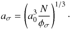 (11)This is calculated for every value of N obtained.
Finally, the size distribution is approximated by a power-law function of the form n(a)da ∝ a− p (Woitke et al. 2016) and then integrated between the maximum and minimum grain size present along the line of sight using the opacity calculator. Therefore, we give as input in the opacity calculator the different grain size distributions.
4.3. Results
Grain growth depends on density, temperature, and dust grain properties. As the temperature and density profiles of L1544 are relatively well known, we can estimate the grain growth in different points of the cloud and predict how much grain size variation is present across the core. We then convolve the modeled distribution with the instrumental beam size to simulate observations.
We consider two scenarios: one where the cloud has not evolved and has maintained its density structure over time, hereafter static cloud, and another where the cloud has evolved and changed its structure with time, hereafter dynamic cloud. In the dynamic scenario, we use the density profiles at different times of evolution of a Bonnor-Ebert sphere in quasi-equilibrium contraction, starting from an unstable dynamical equilibrium state with an initial density of 104 cm-3 as deduced by Keto et al. (2015, their Fig. 3), and stopping when the observed L1544 central density is reached (t ~ 1.06 Myr). The density change is followed in steps by interpolating the various density profiles at different times. Integrating over an interval of time, we can then obtain the grain size distribution evolution starting from an assumed monodisperse initial distribution, and the opacity corresponding to that distribution.
In both cases, the monodisperse distribution starts with a0 = 0.1μm, and follows the grain evolution at every period of time in the Keto et al. (2015) dynamical model. The corresponding opacity maps are convolved with a beam of 20′′ for simulating NIKA observations and of 2′′ to simulate observations with the Atacama Large Millimeter and submillimeter Array (ALMA).
In the static cloud, with the same density and temperature profiles as L1544, dust grains grow in the center up to cm sizes in 1.06 Myr. We consider this result not realistic for two reasons. First, it implies a constant central density of 107 cm-3 for 1.06 Myr, while Keto & Caselli (2010) and Keto et al. (2015) have shown that observed line profiles toward this pre-stellar core are consistent with quasi-equilibrium contraction motions; this dynamical evolution implies central densities larger than 106 cm-3 only in the last ~0.06 Myr. Second, the analytical model overestimates grain growth for densities significantly higher than 105 cm-3. For densities of 106 cm-3 and 107 cm-3, the analytic formula overestimates the grain growth by a factor of ~3 and ~50, respectively, after 1 Myr. In the more realistic dynamical cloud model, the grains reach sizes up to ~230 μm in the core center after a time evolution of 1.06 Myr.
The corresponding opacities at 1.2 mm, which without filtering are proportional to the expected flux, are shown in Figs. 9 and 10 for the static and dynamical cloud, respectively. In the case of a static cloud, the predicted variation in the opacity across the cloud would have been seen with our data, as it predicts a variation of a factor of ~1.5 in the opacity value at NIKA’s resolution. In Fig. 9, it is also evident that there is a drop in opacity when the grains are much larger than the wavelength at which the opacity is derived at ALMA’s resolution, and an enhancement where a ~ λ between 1000 and 2000 au. For the dynamic cloud (Fig. 10), the variation at NIKA’s resolution is not observable with the sensitivity reached as it is below 15%, and the rms of our data corresponds to ~15% of the peak emission. This result is consistent with our observations, which show that no change in the opacity is seen or needed to reproduce the NIKA data. However, Fig. 10 shows that the dust opacity change should be detected with high-resolution telescopes like ALMA as an opacity increase of a factor of 2.5 is predicted toward the central regions of the pre-stellar core. This is a difficult task, as ALMA would filter the extended emission, but the scale we need to look at to find the opacity change is the central 1000–2000 au, and under the right observational configurations (an angular resolution of at least ~5′′ to obtain an expected change in the opacity of a factor of ~2, the inclusion of the Atacama Compact Array and mosaicking) this can be achieved. Therefore, we conclude that ALMA is needed to detect grain growth within pre-stellar cores similar to L1544.
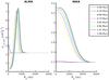 |
Fig. 9 Opacity variation with time and projected radius deduced with ALMA (left) and NIKA (right) simulated observations for the case of a static cloud. The opacity for the NIKA simulated observations changed by a factor of ~1.5, while for ALMA by a factor of ~14. |
 |
Fig. 10 Opacity variation with time and projected radius deduced with ALMA (left) and NIKA (right) simulated observations for the case of a dynamical cloud. The change in the opacity between the center and the outer edge for the case of NIKA is less than 15%, while for ALMA it is a factor of ~2.5 after 1.06 Myr of evolution. |
5. Conclusions
Our work has focused on the search of grain growth toward the central regions of a contracting pre-stellar core, at the earliest phases of the star formation process. We have analyzed the emission from L1544 at 1.2 and 2 mm using the continuum camera at the 30 m IRAM telescope, NIKA. We searched for variation across L1544 on the spectral index and the opacity of the dust as these parameters are sensitive to grain size.
In the derivation of the dust spectral index and opacity, we demonstrate that assumptions on constant dust temperature and spherical symmetry can lead to incorrect conclusions about grain growth.
We investigated the possibility of reproducing, from the model of Keto et al. (2015), the flux seen with NIKA using a constant opacity and spectral index. From the SED fit toward the center of the core using Herschel/SPIRE and NIKA bands, the derived values of κ250 μm and β are: κ250 μm = 0.2 ± 0.1 cm2 g-1 and β = 2.3 ± 0.4. We find that there is no need to increase the opacity toward the central regions to be able to reproduce the observed fluxes. This means that no signatures of grain growth are present toward L1544, within the limits of our data.
Finally, a simple analytical model of grain growth applied to L1544 shows that NIKA observations cannot detect opacity changes across the core and that only interferometers, in particular ALMA, can provide information about grain growth toward the central regions of L1544.
To know the grain size distribution in the earliest phases of star formation is important as the presence of grain growth might affect the future formation of protoplanetary disks and their physical and chemical evolution. In the future, we plan to use ALMA and the Karl G. Jansky Very Large Array (JVLA) data to test our prediction and to extend our study to other dense cores embedded in different environments.
Although different dust-to-gas mass ratios have been measured toward different directions in our Galaxy (Draine 2011), we do not expect significant changes within the same cloud.
The intermediate velocity regime is defined as the velocity range within which the gas-dust friction time is greater than the eddy turnover time. In these conditions, the velocity scales with the square root of the largest particle friction time (Ormel et al. 2009; Ormel & Cuzzi 2007).
The code is available at https://dianaproject.wp.st-andrews.ac.uk/
Acknowledgments
The authors thank the anonymous referee for the careful reading and useful comments, Nicolas Billot for his support and help in the data reduction process, the IRAM 30 m staff, and Jonathan C. Tan and Silvia Spezzano for their useful suggestions. A.C.T., P.C., and J.E.P. acknowledge the financial support of the European Research Council (ERC; project PALs 320620).
References
- Adam, R., Comis, B., Macías-Pérez, J.-F., et al. 2015, A&A, 576, A12 [NASA ADS] [CrossRef] [EDP Sciences] [Google Scholar]
- Adam, R., Bartalucci, I., Pratt, G. W., et al. 2017, A&A, 598, A115 [NASA ADS] [CrossRef] [EDP Sciences] [Google Scholar]
- Agladze, N. I., Sievers, A. J., Jones, S. A., Burlitch, J. M., & Beckwith, S. V. W. 1996, ApJ, 462, 1026 [NASA ADS] [CrossRef] [Google Scholar]
- Andersen, M., Thi, W.-F., Steinacker, J., & Tothill, N. 2014, A&A, 568, L3 [Google Scholar]
- André, P., Men’shchikov, A., Bontemps, S., et al. 2010, A&A, 518, L102 [NASA ADS] [CrossRef] [EDP Sciences] [Google Scholar]
- Bergin, E. A., & Tafalla, M. 2007, ARA&A, 45, 339 [NASA ADS] [CrossRef] [Google Scholar]
- Bertincourt, B., Lagache, G., Martin, P. G., et al. 2016, A&A, 588, A107 [NASA ADS] [CrossRef] [EDP Sciences] [Google Scholar]
- Blum, J. 2004, in Astrophysics of Dust, eds. A. N. Witt, G. C. Clayton, & B. T. Draine, ASP Conf. Ser., 309, 369 [Google Scholar]
- Blum, J., & Schräpler, R. 2004, Phys. Rev. Lett., 93, 115503 [NASA ADS] [CrossRef] [PubMed] [Google Scholar]
- Boogert, A. C. A., Gerakines, P. A., & Whittet, D. C. B. 2015, ARA&A, 53, 541 [Google Scholar]
- Boudet, N., Mutschke, H., Nayral, C., et al. 2005, ApJ, 633, 272 [NASA ADS] [CrossRef] [Google Scholar]
- Brünken, S., Sipilä, O., Chambers, E. T., et al. 2014, Nature, 516, 219 [NASA ADS] [CrossRef] [PubMed] [Google Scholar]
- Calvo, M., Roesch, M., Désert, F.-X., et al. 2013, A&A, 551, L12 [NASA ADS] [CrossRef] [EDP Sciences] [Google Scholar]
- Caselli, P., & Ceccarelli, C. 2012, A&ARv, 20, 56 [NASA ADS] [CrossRef] [MathSciNet] [Google Scholar]
- Caselli, P., Walmsley, C. M., Tafalla, M., Dore, L., & Myers, P. C. 1999, ApJ, 523, L165 [NASA ADS] [CrossRef] [Google Scholar]
- Caselli, P., Keto, E., Bergin, E. A., et al. 2012, ApJ, 759, L37 [Google Scholar]
- Catalano, A., Calvo, M., Ponthieu, N., et al. 2014, A&A, 569, A9 [NASA ADS] [CrossRef] [EDP Sciences] [Google Scholar]
- Coupeaud, A., Demyk, K., Meny, C., et al. 2011, A&A, 535, A124 [NASA ADS] [CrossRef] [EDP Sciences] [Google Scholar]
- Crapsi, A., Caselli, P., Walmsley, C. M., et al. 2005, ApJ, 619, 379 [Google Scholar]
- Crapsi, A., Caselli, P., Walmsley, M. C., & Tafalla, M. 2007, A&A, 470, 221 [NASA ADS] [CrossRef] [EDP Sciences] [Google Scholar]
- Demyk, K., Meny, C., Leroux, H., et al. 2013, in Proc. of The Life Cycle of Dust in the Universe: Observations, Theory, and Laboratory Experiments (LCDU2013), 18–22 November, 2013, Taipei, Taiwan, eds. A. Andersen, M. Baes, H. Gomez, C. Kemper & D. Watson, PoS(LCDU2013)044 [Google Scholar]
- Dorschner, J., Begemann, B., Henning, T., Jaeger, C., & Mutschke, H. 1995, A&A, 300, 503 [NASA ADS] [Google Scholar]
- Draine, B. T. 2006, ApJ, 636, 1114 [NASA ADS] [CrossRef] [Google Scholar]
- Draine, B. T. 2011, Physics of the Interstellar and Intergalactic Medium (Princeton University Press) [Google Scholar]
- Forbrich, J., Lada, C. J., Lombardi, M., Román-Zúñiga, C., & Alves, J. 2015, A&A, 580, A114 [NASA ADS] [CrossRef] [EDP Sciences] [Google Scholar]
- Foster, J. B., Mandel, K. S., Pineda, J. E., et al. 2013, MNRAS, 428, 1606 [NASA ADS] [CrossRef] [Google Scholar]
- Hildebrand, R. H. 1983, QJRAS, 24, 267 [NASA ADS] [Google Scholar]
- Jones, A. P., Fanciullo, L., Köhler, M., et al. 2013, A&A, 558, A62 [NASA ADS] [CrossRef] [EDP Sciences] [Google Scholar]
- Juvela, M., Demyk, K., Doi, Y., et al. 2015a, A&A, 584, A94 [NASA ADS] [CrossRef] [EDP Sciences] [Google Scholar]
- Juvela, M., Ristorcelli, I., Marshall, D. J., et al. 2015b, A&A, 584, A93 [NASA ADS] [CrossRef] [EDP Sciences] [Google Scholar]
- Kauffmann, J., Bertoldi, F., Bourke, T. L., Evans, II, N. J., & Lee, C. W. 2008, A&A, 487, 993 [NASA ADS] [CrossRef] [EDP Sciences] [Google Scholar]
- Keto, E., & Caselli, P. 2010, MNRAS, 402, 1625 [NASA ADS] [CrossRef] [Google Scholar]
- Keto, E., Caselli, P., & Rawlings, J. 2015, MNRAS, 446, 3731 [NASA ADS] [CrossRef] [Google Scholar]
- Köhler, M., Ysard, N., & Jones, A. P. 2015, A&A, 579, A15 [NASA ADS] [CrossRef] [EDP Sciences] [Google Scholar]
- Kong, S., Caselli, P., Tan, J. C., Wakelam, V., & Sipilä, O. 2015, ApJ, 804, 98 [NASA ADS] [CrossRef] [Google Scholar]
- Könyves, V., André, P., Men’shchikov, A., et al. 2015, A&A, 584, A91 [NASA ADS] [CrossRef] [EDP Sciences] [Google Scholar]
- Kruegel, E., & Siebenmorgen, R. 1994, A&A, 288, 929 [NASA ADS] [Google Scholar]
- Lefèvre, C., Pagani, L., Min, M., Poteet, C., & Whittet, D. 2016, A&A, 585, L4 [NASA ADS] [CrossRef] [EDP Sciences] [Google Scholar]
- Mennella, V., Brucato, J. R., Colangeli, L., et al. 1998, ApJ, 496, 1058 [NASA ADS] [CrossRef] [Google Scholar]
- Min, M., Hovenier, J. W., de Koter, A., Waters, L. B. F. M., & Dominik, C. 2005, Icarus, 179, 158 [NASA ADS] [CrossRef] [Google Scholar]
- Miyake, K., & Nakagawa, Y. 1993, Icarus, 106, 20 [NASA ADS] [CrossRef] [Google Scholar]
- Natta, A., & Testi, L. 2004, in Star Formation in the Interstellar Medium: In Honor of David Hollenbach, eds. D. Johnstone, F. C. Adams, D. N. C. Lin, D. A. Neufeeld, & E. C. Ostriker, ASP Conf. Ser., 323, 279 [Google Scholar]
- Ormel, C. W., & Cuzzi, J. N. 2007, A&A, 466, 413 [NASA ADS] [CrossRef] [EDP Sciences] [Google Scholar]
- Ormel, C. W., Paszun, D., Dominik, C., & Tielens, A. G. G. M. 2009, A&A, 502, 845 [NASA ADS] [CrossRef] [EDP Sciences] [Google Scholar]
- Ormel, C. W., Min, M., Tielens, A. G. G. M., Dominik, C., & Paszun, D. 2011, A&A, 532, A43 [NASA ADS] [CrossRef] [EDP Sciences] [Google Scholar]
- Ossenkopf, V. 1993, A&A, 280, 617 [NASA ADS] [Google Scholar]
- Ossenkopf, V., & Henning, T. 1994, A&A, 291, 943 [NASA ADS] [Google Scholar]
- Pagani, L., Steinacker, J., Bacmann, A., Stutz, A., & Henning, T. 2010, Science, 329, 1622 [NASA ADS] [CrossRef] [PubMed] [Google Scholar]
- Planck Collaboration X. 2016, A&A, 594, A10 [NASA ADS] [CrossRef] [EDP Sciences] [Google Scholar]
- Sadavoy, S. I., Stutz, A. M., Schnee, S., et al. 2016, A&A, 588, A30 [NASA ADS] [CrossRef] [EDP Sciences] [Google Scholar]
- Schnee, S., & Goodman, A. 2005, ApJ, 624, 254 [NASA ADS] [CrossRef] [Google Scholar]
- Schnee, S., Mason, B., Di Francesco, J., et al. 2014, MNRAS, 444, 2303 [NASA ADS] [CrossRef] [Google Scholar]
- Shetty, R., Kauffmann, J., Schnee, S., & Goodman, A. A. 2009a, ApJ, 696, 676 [NASA ADS] [CrossRef] [Google Scholar]
- Shetty, R., Kauffmann, J., Schnee, S., Goodman, A. A., & Ercolano, B. 2009b, ApJ, 696, 2234 [NASA ADS] [CrossRef] [Google Scholar]
- Spezzano, S., Bizzocchi, L., Caselli, P., Harju, J., & Brünken, S. 2016, A&A, 592, L11 [CrossRef] [EDP Sciences] [Google Scholar]
- Testi, L., Birnstiel, T., Ricci, L., et al. 2014, Protostars and Planets VI, 339 [Google Scholar]
- Toon, O. B., & Ackerman, T. P. 1981, Appl. Opt., 20, 3657 [Google Scholar]
- Wang, K., Testi, L., Ginsburg, A., et al. 2015, MNRAS, 450, 4043 [NASA ADS] [CrossRef] [MathSciNet] [Google Scholar]
- Ward-Thompson, D., Motte, F., & Andre, P. 1999, MNRAS, 305, 143 [NASA ADS] [CrossRef] [Google Scholar]
- Woitke, P., Min, M., Pinte, C., et al. 2016, A&A, 586, A103 [NASA ADS] [CrossRef] [EDP Sciences] [Google Scholar]
- Zhao, B., Caselli, P., Li, Z.-Y., et al. 2016, MNRAS, 460, 2050 [NASA ADS] [CrossRef] [Google Scholar]
- Zubko, V. G., Mennella, V., Colangeli, L., & Bussoletti, E. 1996, MNRAS, 282, 1321 [NASA ADS] [CrossRef] [Google Scholar]
Appendix A: NIKA and Herschel/SPIRE filtering
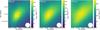 |
Fig. A.1 Original Herschel/SPIRE maps after smoothing to the lowest resolution and before applying any filtering method. The contours represent steps of 25% of the peak emission at each band. The HPBW, which corresponds to the higher resolution of Herschel/SPIRE (38.5′′), is shown by the white circle in the bottom right corner. |
Sadavoy et al. (2016) presented a way to filter Herschel/SPIRE large scale emission, based on the work of Wang et al. (2015), by cutting off the low spatial frequencies in the Fourier domain based on their GISMO 2 mm data. To study this method with our data, we smoothed all the bands to the lowest resolution (~38.5′′, corresponding to the 500 μm SPIRE band; these maps can be seen in Fig. A.1) and performed a Fourier transform on all the maps. We then obtained the radial amplitude profile of the 2 mm frequency domain maps by averaging in rings one pixel wide, as done in Sadavoy et al. (2016). This profile is shown in Fig. A.2, together with that at 1.2 mm for comparison. This profile is then fitted with an exponential function, and the fit is used to construct a mask for SPIRE maps in the same manner as described in Sadavoy et al. (2016).
There is not much difference between using the 1.2 mm map and the 2 mm map as a mask as both profiles have identical slopes within the errors (see Fig. A.2). This is also an indication of similar filtering in both bands, as expected from the similarity of the fields of view and as predicted by Adam et al. (2015).
The final filtered SPIRE maps are shown in Fig. A.3 for the Fourier transform method and in Fig. A.4 for the method used in this work (see Sect. 2.2), where an aperture is chosen to subtract the emission from the original maps. In the first case, they show very centrally concentrated emission with a decrease in the peak surface brightness of 40, 60, and 50% for the 500, 350, and 250 μm bands, respectively, with respect to the original SPIRE maps. The peak emission we obtained with the aperture filtering method, compared with the Fourier transform method results, gives differences of approximately 30, 25, and 40% for the 500, 350, and 250 μm bands, respectively. As the two shorter wavelengths bands see an increase in surface brightness, there is an increase in the spectral index and the opacity, obtaining in this case β = 2.5 ± 0.6 and κ250 μm = 0.28 ± 0.14 cm2 g-1. Although this is still within our uncertainties, this opacity and spectral index do not reproduce the observed NIKA millimeter emission as accurately: the ratio between the observed emission and the model is 1.3 in both cases. This difference can be due to the high concentration of emission in the central pixel, and this may be a source of error. It could artificially increase the peak emission, making the slope of the spectral energy distribution increase as well. We therefore used the method that reproduces the millimeter observations more closely, although the two methods give similar results within the uncertainties.
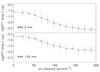 |
Fig. A.2 Fourier amplitude profiles of the 1.2 mm (top) and 2 mm (bottom) data in the frequency domain. The profiles are obtained by averaging in rings of 1 pixel in width at different distances from the center of the Fourier transformed emission maps. The profile at 2 mm is used to derive a mask, which is applied to the Herschel/SPIRE data in order to filter out the large-scale emission. |
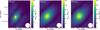 |
Fig. A.3 Resulting Herschel/SPIRE maps after applying the filtering method from Sadavoy et al. (2016). The contours represent steps of 25% of the peak emission at each band. The emission is seen to be centrally concentrated in the central pixels. |
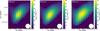 |
Fig. A.4 Resulting Herschel/SPIRE maps after applying the filtering method used in this work, extracting the emission around the core where no emission is detected in mm wavelengths. The contours represent steps of 25% of the peak emission at each band. |
All Figures
|
Fig. 1 Maps of the continuum emission of L1544 at a) 1.2 mm and b) 2 mm. The angular resolution is 12.5′′ at 1.2 mm and 18.5′′ at 2 mm (HPBW shown by the white circle in the bottom right corner) and the contours are indicating the different σ levels of the emission above 3σ (3σ, 4σ, 5σ, etc., where σ1.2 mm = 1.4 MJy/sr and σ2 mm = 0.15 MJy/sr). |
| In the text | |
|
Fig. 2 Maps of the a) spectral index and b) opacity at 1.2 mm assuming a constant core temperature of 10 K and a constant κ250 μm = 0.1 cm2 g-1 value (Hildebrand 1983). The 1.2 mm map was convolved to the 2 mm band resolution, which is 19′′ (HPBW shown by the white circle in the bottom right corner). In both cases, the crosses mark the peak of the emission corresponding to the final 1.2 mm map convolved to 19′′. |
| In the text | |
|
Fig. 3 Temperature (red) and density (blue) profiles of L1544 from Keto et al. (2015). |
| In the text | |
|
Fig. 4 Maps of the a) spectral index and b) opacity at 1.2 mm derived with the method described in Sect. 3.2.2. The angular resolution is 19′′ (HPBW shown by the white circle in the bottom right corner). The crosses mark the peak of the emission corresponding to the final 1.2 mm map convolved to 19′′. |
| In the text | |
|
Fig. 5 Fit of the SED to the five spectral windows available at 250, 350, 500, 1250, and 2000 μm at the peak emission when convolving and regridding all windows to the resolution of the 500 μm band. The error bars indicate the weights used in the fitting, which correspond to the uncertainties and noise associated with the data. The shadowed blue region show the 95% confidence intervals of the fitted parameters. |
| In the text | |
|
Fig. 6 Ellipses where the emission has been averaged for the 1.2 mm and 2 mm maps superimposed on the 1.2 mm continuum map of L1544. Only the colored region is included in the average. The resolution is 19′′ (HPBW shown by the black circle in the bottom right corner). For Herschel/SPIRE the distance between concentric ellipses is larger, due to a larger pixel size and resolution. For both NIKA and SPIRE, the distance between ellipses is chosen to be ~1.8 pixels, averaging in a 1 pixel wide ring. |
| In the text | |
|
Fig. 7 Ratio between the observed and the modeled surface brightnesses at 1.2 mm (top) and 2 mm (bottom) as a function of geometric mean radius of the ellipses in Fig. 6, using the temperature and density profiles from Keto et al. (2015) and an opacity value of κ250 μm = 0.2 ± 0.1 cm2 g-1 and β = 2.3 ± 0.4. The shadowed red region represents the uncertainties on the fluxes, the opacity, and the spectral index. The shaded blue region indicates the zone where the observed surface brightness is below 3σ. |
| In the text | |
|
Fig. 8 Ratio between the observed and the modeled surface brightnesses at 500 μm (top), 350 μm (middle), and 250 μm (bottom) as a function of the geometric mean radius of the ellipses, as explained in Fig. 6, using the temperature and density profiles from Keto et al. (2015) and an opacity value of κ250 μm = 0.2 ± 0.1 cm2 g-1 and β = 2.3 ± 0.4. The shadowed red region represents the uncertainties on the fluxes, the opacity, and the spectral index. The shaded blue region indicates the zone where the millimeter observed surface brightness is below 3σ as the artificial filtering of Herschel/SPIRE relies on the shape of the 1.2 mm emission (see Sect. 2.2 and Appendix A). |
| In the text | |
|
Fig. 9 Opacity variation with time and projected radius deduced with ALMA (left) and NIKA (right) simulated observations for the case of a static cloud. The opacity for the NIKA simulated observations changed by a factor of ~1.5, while for ALMA by a factor of ~14. |
| In the text | |
|
Fig. 10 Opacity variation with time and projected radius deduced with ALMA (left) and NIKA (right) simulated observations for the case of a dynamical cloud. The change in the opacity between the center and the outer edge for the case of NIKA is less than 15%, while for ALMA it is a factor of ~2.5 after 1.06 Myr of evolution. |
| In the text | |
|
Fig. A.1 Original Herschel/SPIRE maps after smoothing to the lowest resolution and before applying any filtering method. The contours represent steps of 25% of the peak emission at each band. The HPBW, which corresponds to the higher resolution of Herschel/SPIRE (38.5′′), is shown by the white circle in the bottom right corner. |
| In the text | |
|
Fig. A.2 Fourier amplitude profiles of the 1.2 mm (top) and 2 mm (bottom) data in the frequency domain. The profiles are obtained by averaging in rings of 1 pixel in width at different distances from the center of the Fourier transformed emission maps. The profile at 2 mm is used to derive a mask, which is applied to the Herschel/SPIRE data in order to filter out the large-scale emission. |
| In the text | |
|
Fig. A.3 Resulting Herschel/SPIRE maps after applying the filtering method from Sadavoy et al. (2016). The contours represent steps of 25% of the peak emission at each band. The emission is seen to be centrally concentrated in the central pixels. |
| In the text | |
|
Fig. A.4 Resulting Herschel/SPIRE maps after applying the filtering method used in this work, extracting the emission around the core where no emission is detected in mm wavelengths. The contours represent steps of 25% of the peak emission at each band. |
| In the text | |
Current usage metrics show cumulative count of Article Views (full-text article views including HTML views, PDF and ePub downloads, according to the available data) and Abstracts Views on Vision4Press platform.
Data correspond to usage on the plateform after 2015. The current usage metrics is available 48-96 hours after online publication and is updated daily on week days.
Initial download of the metrics may take a while.