© ESO, 2017

1. Introduction

In galaxy clusters, temperature and density are the key observable characteristics of the hot ionised gas in the intracluster medium (ICM). X-ray observations play a fundamental role in their measurement. Density is trivial to obtain from X-ray imaging, while temperature can be derived from an isothermal model fit to the spectrum. Accurate gas temperatures are needed for a number of reasons. Accurate temperatures are essential to infer cluster masses under the assumption of hydrostatic equilibrium (Sarazin 1988); in turn, these masses can be used to infer constraints on cosmological parameters (e.g. Allen et al. 2011). The temperature structure yields information on the detailed physics of shock-heated gas in merging events, the nature of cold fronts, and the role of turbulence and gas sloshing (see e.g. Markevitch & Vikhlinin 2007, for a review). In turn, such analyses provide insights into the assembly physics of galaxy clusters, which is necessary to interpret the scaling relations between clusters masses and their primary observables (Khedekar et al. 2013).

However, the X-ray gas temperature measurement is potentially affected by two systematic effects. First, the X-ray emission is proportional to the square of the ICM electron density, such that spectroscopic temperatures are driven by the colder, denser regions along the line of sight and are thus sensitive to gas clumping. In fact, a weighted mean temperature is measured, in which the weight is a non-linear combination of the temperature and density structure (see e.g. Mazzotta et al. 2004; Vikhlinin 2006). Numerical simulations support this view (e.g. Nagai et al. 2007; Rasia et al. 2014), but estimates of the magnitude of any bias due to this effect vary widely depending on the numerical scheme (e.g. smoothed particle hydrodynamics, adaptive mesh refinement) and the details of sub-grid physics (cooling, feedback, etc.). Secondly, the spectroscopic temperatures depend directly on the energy calibration of X-ray observatories. For instance, X-ray temperatures obtained with Chandra are generally higher than those measured by XMM-Newton by up to a factor of 15% at 10 keV (e.g. Mahdavi et al. 2013).

The thermal Sunyaev-Zel’dovich (tSZ; Sunyaev & Zeldovich 1972) effect is related to the mean gas-mass-weighted temperature along the line of sight and the electron density, via the ideal gas law. The tSZ effect can thus be used to obtain an alternative estimate of the gas temperature provided that a measure of the density is available. A combination of the tSZ and X-ray observations can then in principle be used to decouple temperature and density in each individual measurement. Such a method has previously been used to extract 1D gas temperature profiles, complementing X-ray spectroscopic measurements (e.g. Pointecouteau et al. 2002; Kitayama et al. 2004; Nord et al. 2009; Basu et al. 2010; Eckert et al. 2013; Ruppin et al. 2017).

Here, we explore the application of the method to 2D data. We use deep, resolved (<20″) tSZ observations, combined with X-ray imaging, to measure the spatial distribution of the gas temperature towards the merging cluster MACS J0717.5+3745 at z = 0.55. We chose MACS J0717.5+3745 as a test case cluster because it is one of the very few objects for which tSZ data of sufficient depth and resolution are currently available (Adam et al. 2017). The complex morphology of the cluster is the primary limiting factor to our analysis; however the system allows us to explore a wide range of gas temperatures, which are not necessarily accessible with more simple objects. We compare our new temperature map, based on X-ray and tSZ imaging, to that obtained from application of standard X-ray spectroscopic techniques using XMM-Newton and Chandra data. We describe and discuss in detail the various factors affecting the ratio between the two temperature estimates. We assume a flat ΛCDM cosmology according to the latest Planck results (Planck Collaboration XIII 2016) with H₀ = 67.8 km s^-1 Mpc^-1, Ω_M = 0.308, and Ω_Λ = 0.692. At the cluster redshift, 1 arcsec corresponds to 6.6 kpc.

2. Data

The New IRAM KIDs Array (NIKA; see Monfardini et al. 2011; Calvo et al. 2013; Adam et al. 2014; Catalano et al. 2014) has observed MACS J0717.5+3745 at 150 and 260 GHz for a total of 47.2 ks. The main steps of the data reduction are described in Adam et al. (2015, 2016, 2017), Ruppin et al. (2017). In this paper, we use the NIKA 150 GHz tSZ map at 22 arcsec effective angular resolution full width half maximum (FWHM), deconvolved from the transfer function except for the beam smoothing. The overall calibration uncertainty is estimated to be 7%, including the brightness temperature model of our primary calibrator, the NIKA bandpass uncertainties, the opacity correction, and the stability of the instrument (Catalano et al. 2014). The absolute zero level for the brightness on the map remains unconstrained by NIKA. MACS J0717.5+3745 is contaminated by a significant amount of kinetic SZ (kSZ; Sunyaev & Zeldovich 1980) signal and we used the best-fit model F2 from Adam et al. (2017) to remove its contribution. This model has large uncertainties but it still allows us to test the impact of the kSZ effect on our results.

MACS J0717.5+3745 was observed several times by the XMM-Newton and Chandra X-ray observatories (obs-IDs 0672420101, 0672420201, 067242030, and 1655, 4200, 16235, 16305, respectively). The data processing follows the description given in Adam et al. (2017). The clean exposure time is 153 ks for Chandra and 160 and 116 ks for XMM-Newton MOS1, 2 and PN cameras, respectively.

3. Temperature reconstruction

The method employed to recover the temperature of the gas from NIKA tSZ and XMM-Newton X-ray imaging, T_SZX, is described below. The X-ray spectroscopic temperature mapping method is discussed in Sect. 3.6 and Appendix A.

3.1. Primary observables

The tSZ signal, measured at frequency ν, can be expressed as 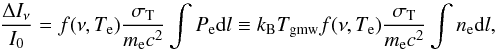$\frac{\mathrm{\Delta }{\mathit{I}}_{\mathit{\nu }}}{{\mathit{I}}_{\mathrm{0}}}\mathrm{=}\mathit{f}\mathrm{\left(}\mathit{\nu ,}{\mathit{T}}_{\mathrm{e}}\mathrm{\right)}\frac{{\mathit{\sigma }}_{\mathrm{T}}}{{\mathit{m}}_{\mathrm{e}}{\mathit{c}}^{\mathrm{2}}}\mathrm{\int }{\mathit{P}}_{\mathrm{e}}\mathrm{d}\mathit{l}\mathrm{\equiv }{\mathit{k}}_{\mathrm{B}}{\mathit{T}}_{\mathrm{gmw}}\mathit{f}\mathrm{\left(}\mathit{\nu ,}{\mathit{T}}_{\mathrm{e}}\mathrm{\right)}\frac{{\mathit{\sigma }}_{\mathrm{T}}}{{\mathit{m}}_{\mathrm{e}}{\mathit{c}}^{\mathrm{2}}}\mathrm{\int }{\mathit{n}}_{\mathrm{e}}\mathrm{d}\mathit{l,}$(1)where f(ν,T_e) is the tSZ spectrum, which depends slightly on temperature T_e in the case of very hot gas. The signal is proportional to the line of sight integrated electron pressure, P_e. It is related to the mean gas-mass-weighted temperature along the line of sight, ${\mathit{T}}_{\mathrm{gmw}}\mathrm{\equiv }\frac{\mathrm{\int }{\mathit{T}}_{\mathrm{e}}{\mathit{n}}_{\mathrm{e}}\mathrm{d}\mathit{l}}{\mathrm{\int }{\mathit{n}}_{\mathrm{e}}\mathrm{d}\mathit{l}}\mathit{,}$(2)and the electron density, n_e, via the ideal gas law. The X-ray surface brightness is driven by the electron density ${\mathit{S}}_{\mathrm{X}}\mathrm{=}\frac{\mathrm{1}}{\mathrm{4}\mathit{\pi }{\mathrm{(}\mathrm{1}\mathrm{+}{\mathit{z}}^{\mathrm{)}}}^{\mathrm{4}}}\mathrm{\int }{\mathit{n}}_{\mathrm{e}}^{\mathrm{2}}\mathrm{\Lambda }\mathrm{\left(}{\mathit{T}}_{\mathrm{e}}\mathit{,Z}\mathrm{\right)}\mathrm{d}\mathit{l,}$(3)where z is the cluster redshift and Λ(T_e,Z) is the emissivity in the relevant energy band, taking into account the interstellar absorption and instrument spectral response. The parameter Λ(T_e,Z) depends only weakly on the temperature and metallicity of the gas Z, so that instrumental systematics have a negligible impact on the results presented in this paper.

3.2. X-ray electron density mapping

We used the XMM-Newton X-ray surface brightness (Eq. (3)) to produce a map of the square of the electron density integrated along the line of sight, ${}^{\mathrm{\int }}\mathit{n}_{\mathrm{e}}^{\mathrm{2}}\mathrm{d}\mathit{l}$. To combine it with tSZ observations, we had to convert ${}^{\mathrm{\int }}\mathit{n}_{\mathrm{e}}^{\mathrm{2}}\mathrm{d}\mathit{l}$ to ${}^{\mathrm{\int }}\mathit{n}_{\mathrm{e}}\mathrm{d}\mathit{l}$ via an effective electron depth, expressed as ${\mathit{\ell }}_{\mathrm{eff}}\mathrm{=}\frac{{{\mathrm{(}}^{\mathrm{\int }}{\mathit{n}}_{\mathrm{e}}\mathrm{d}{\mathit{l}}^{\mathrm{)}}}^{\mathrm{2}}}{\mathrm{\int }{\mathit{n}}_{\mathrm{e}}^{\mathrm{2}}\mathrm{d}\mathit{l}}\mathrm{·}$(4)From Eq. (3), the average density along the line of sight is then given by 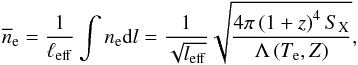${\overline{\mathit{n}}}_{\mathrm{e}}\mathrm{=}\frac{\mathrm{1}}{{\mathit{\ell }}_{\mathrm{eff}}}\mathrm{\int }{\mathit{n}}_{\mathrm{e}}\mathrm{d}\mathit{l}\mathrm{=}\frac{\mathrm{1}}{\sqrt{{\mathit{l}}_{\mathrm{eff}}}}\sqrt{\frac{\mathrm{4}\mathit{\pi }{\mathrm{(}\mathrm{1}\mathrm{+}{\mathit{z}}^{\mathrm{)}}}^{\mathrm{4}}{\mathit{S}}_{\mathrm{X}}}{\mathrm{\Lambda }\mathrm{(}{\mathit{T}}_{\mathrm{e}}\mathit{,}{\mathit{Z}}^{\mathrm{)}}}}\mathit{,}$(5)defining an effective density.

3.3. Thermal Sunyaev-Zel’dovich pressure mapping

Similarly, we can express the effective pressure along the line of sight directly from Eq. (1), as 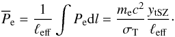${\overline{\mathit{P}}}_{\mathrm{e}}\mathrm{=}\frac{\mathrm{1}}{{\mathit{\ell }}_{\mathrm{eff}}}\mathrm{\int }{\mathit{P}}_{\mathrm{e}}\mathrm{d}\mathit{l}\mathrm{=}\frac{{\mathit{m}}_{\mathrm{e}}{\mathit{c}}^{\mathrm{2}}}{{\mathit{\sigma }}_{\mathrm{T}}}\frac{{\mathit{y}}_{\mathrm{tSZ}}}{{\mathit{\ell }}_{\mathrm{eff}}}\mathrm{·}$(6)We obtained this quantity in straightforward way from the NIKA map accounting for relativistic corrections as detailed in Adam et al. (2017). As the temperature can be very high, the relativistic corrections are non-negligible (Pointecouteau et al. 1998; Itoh & Nozawa 2003), but the exact choice of the temperature map used to apply relativistic corrections has a negligible impact on our results (i.e. the spectroscopic temperature maps from XMM-Newton, Chandra, or T_SZX).

3.4. Gas-mass-weighted temperature mapping

We obtained the tSZ+X-ray imaging temperature map, T_SZX, by combining the effective density and pressure 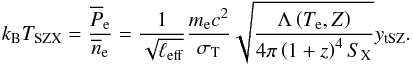${\mathit{k}}_{\mathrm{B}}{\mathit{T}}_{\mathrm{SZX}}\mathrm{=}\frac{{\overline{\mathit{P}}}_{\mathrm{e}}}{{\overline{\mathit{n}}}_{\mathrm{e}}}\mathrm{=}\frac{\mathrm{1}}{\sqrt{{\mathit{\ell }}_{\mathrm{eff}}}}\frac{{\mathit{m}}_{\mathrm{e}}{\mathit{c}}^{\mathrm{2}}}{{\mathit{\sigma }}_{\mathrm{T}}}\sqrt{\frac{\mathrm{\Lambda }\mathrm{(}{\mathit{T}}_{\mathrm{e}}\mathit{,}{\mathit{Z}}^{\mathrm{)}}}{\mathrm{4}\mathit{\pi }{\mathrm{(}\mathrm{1}\mathrm{+}{\mathit{z}}^{\mathrm{)}}}^{\mathrm{4}}{\mathit{S}}_{\mathrm{X}}}}{\mathit{y}}_{\mathrm{tSZ}}\mathit{.}$(7)The temperature map T_SZX is an estimate of the gas-mass-weighted temperature, T_gmw (Eq. (2)). We propagated the noise arising from the tSZ map and the X-ray surface brightness with Monte Carlo realisations; the overall noise on T_SZX is dominated by that of the tSZ map. The sources of systematic errors are incorrect modelling of ℓ_eff along with tSZ calibration uncertainties and contamination from the kSZ effect. The absolute calibration error of the X-ray flux is expected to be negligible.

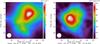Fig. 1 Left: effective line of sight electron density, ${\overline{\mathit{n}}}_{\mathrm{e}}$, derived from XMM-Newton. Right: effective line of sight pressure, ${\overline{\mathit{P}}}_{\mathrm{e}}$, derived from NIKA is shown. These maps correspond to model M1, and were smoothed with a Gaussian kernel to an effective resolution of 22 arcsec FWHM. The pressure map is cleaned from our best-fit kSZ model and corrected for the zero level.

3.5. Effective electron depth

The effective electron depth is a key quantity for the method, as the derived gas-mass-weighted temperature scales with $\sqrt{{\mathit{\ell }}_{\mathrm{eff}}}$. It can be re-expressed as ${\mathit{\ell }}_{\mathrm{eff}}\mathrm{=}\frac{{\mathit{R}}_{\mathrm{500}}}{{\mathit{Q}}_{{\mathit{n}}_{\mathrm{e}}}^{\mathrm{2}}}\mathrm{with}{\mathit{Q}}_{{\mathit{n}}_{\mathrm{e}}}\mathrm{=}\frac{\sqrt{\mathrm{⟨}{\mathit{n}}_{\mathrm{e}}^{\mathrm{2}}\mathrm{⟩}}}{\mathrm{⟨}{\mathit{n}}_{\mathrm{e}}\mathrm{⟩}}\mathit{,}$(8)where the brackets denote averaging along the line of sight, carried out in scaled coordinates. The electron depth at each projected position depends, via the shape factor Q_ne, on the geometry of the gas density distribution at all scales, from the large-scale radial dependence to small-scale fluctuations. In particular, Q_ne increases with increasing gas concentration and clumpiness.

In the following, we used several approaches to estimate ℓ_eff and its uncertainty:

• 1.

  Model M1: following Sayerset al. (2013), we assumed thatℓ_eff is constant at ℓ_eff = 1400 kpc, as estimated by Mroczkowski et al. (2012), across the cluster extension.

• 2.

  Model M2: we derived an electron density profile from deconvolution and deprojection of the XMM-Newton radial S_X profile centred on the X-ray peak (Croston et al. 2006), thus obtaining an azimuthally symmetric ℓ_eff map.

• 3.

  Model M3: we used the best-fitting NIKA tSZ and XMM-Newton density model of Adam et al. (2017), which accounts for the four main subclusters in MACS J0717.5+3745, to compute a map of ℓ_eff. The model does not constrain the line of sight distance between the subclusters because the tSZ signal depends linearly on the density. Therefore, we considered two extreme cases: M3a) where the subclusters are sufficiently far away from each other such that ${}^{\mathrm{\int }}\mathit{n}_{\mathrm{e}}^{\mathrm{2}}\mathrm{d}\mathit{l}\mathrm{\simeq }{\sum }_{\mathit{j}}{}^{\mathrm{\int }}\mathit{n}_{\mathrm{e}\mathit{,j}}^{\mathrm{2}}\mathrm{d}\mathit{l}$, where j refers to each subcluster; M3b) where all the subclusters are located in the same plane, perpendicular to the line of sight. The physical distances between the subclusters are thus minimal, maximizing the ${}^{\mathrm{\int }}\mathit{n}_{\mathrm{e}}^{\mathrm{2}}\mathrm{d}\mathit{l}$ integral.

While the internal structure of MACS J0717.5+3745 is increasingly refined from model M1 to M3, we found good consistency between all three models. Model M2 presents a minimum of 1200 kpc towards the X-ray centre and increases quasi-linearly towards higher radii, reaching about 2000 kpc at 1 arcmin, in line with expectations from model M1. Model M3a is minimal in the central region in the direction of the subclusters (~ 1200 kpc) and also increases with radius. Model M3b provides a lower limit for ℓ_eff, increasing from ~ 800 kpc near the centre to ~ 1200 kpc at 1 arcmin.

While these models allowed us to test the impact of the gas geometry on large scales, they do not specifically account for clumping on small scales. Despite the weak dependence of the gas-mass-weighted temperature on the electron depth (∝$\sqrt{{\mathit{\ell }}_{\mathrm{eff}}}$), clumping might affect our results. We discuss this further in Sect. 4.

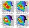Fig. 2 Temperature maps. Top: spectroscopic temperature derived from Chandra (TCXO, left panel) and from XMM-Newton (TXMM, right panel) are shown. Bottom: NIKA and XMM-Newton imaging derived temperature, TSZX, for model M1 (left panel) and model M3a (right panel) are shown. These maps are corrected for the zero level.

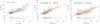Fig. 3 Correlation between the temperature maps of Fig. 2 and residual. Left: XMM-Newton vs. Chandra spectroscopic temperatures is shown. Middle: tSZ+X-ray imaging (model M1) vs. XMM-Newton spectroscopy is shown. Right: tSZ+X-ray imaging (model M1) vs. Chandra spectroscopy is shown. The red and green dots correspond to the case with and without the kSZ correction, respectively.

3.6. X-ray spectroscopic temperature maps

The X-ray spectroscopic temperature maps from Chandra (T_CXO) and XMM-Newton (T_XMM) were produced using the wavelet filtering algorithm described in Bourdin & Mazzotta (2008), as detailed in Adam et al. (2017). As the significance of wavelet coefficients partly depends on the photon count statistics, the effective resolution varies across the map, XMM-Newton allowing a finer sampling than Chandra owing to a higher effective area. We estimated the uncertainties per map pixel using a Monte Carlo approach, as discussed in Appendix A.

Comparison of the temperature derived from tSZ+X-ray imaging to the X-ray spectroscopic temperature provides further information on the ICM structure and on calibration systematics. From Eqs. (7) and (8), at each projected position the ratio of the two temperatures can be expressed as 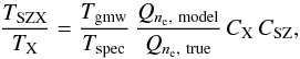$\frac{{\mathit{T}}_{\mathrm{SZX}}}{{\mathit{T}}_{\mathrm{X}}}\mathrm{=}\frac{{\mathit{T}}_{\mathrm{gmw}}}{{\mathit{T}}_{\mathrm{spec}}}\hspace{0.17em}\frac{{\mathit{Q}}_{{\mathit{n}}_{\mathrm{e}}\mathit{,}\mathrm{model}}}{{\mathit{Q}}_{{\mathit{n}}_{\mathrm{e}}\mathit{,}\mathrm{true}}}\hspace{0.17em}{\mathit{C}}_{\mathrm{X}}\hspace{0.17em}{\mathit{C}}_{\mathrm{SZ}}\mathit{,}$(9)where T_gmw is the true gas-mass-weighted temperature and T_spec is the spectroscopic temperature that would be obtained by fitting an isothermal model to the observed spectra for a perfectly calibrated instrument. The value C_X = T_spec/T_X is the ratio between the latter and the measured X-ray temperature, which accounts for the X-ray calibration uncertainty. The value C_SZ accounts for the tSZ calibration.

The measured ratio T_SZX/T_X is an estimate of the ratio between the gas-mass-weighted temperature and the spectroscopic temperature, Q_T = T_gmw/T_spec. The spectroscopic temperature T_spec is expected to be biased low as compared to the gas-mass-weighted temperature and depends on the instrument used to make the measurement. The ratio Q_T is a shape parameter, which depends on both the density and temperature structure along the line of sight. In addition to calibration issues, the measured ratio T_SZX/T_X may differ from Q_T if the density shape factor, Q_ne, is incorrect. For a given cluster, the various terms on the right-hand side of Eq. (9) are in principle degenerate. Part of the degeneracy, in particular of calibration versus physical factors, can be broken by taking into account the expected differences in spatial dependence.

4. Results

4.1. Morphology

The left and right panels of Fig. 1 represent the effective density and pressure maps in the case of the simplest model M1, thus $\mathrm{\propto }\sqrt{{}^{\mathrm{\int }}\mathit{n}_{\mathrm{e}}^{\mathrm{2}}\mathrm{d}\mathit{l}}$ and ∝${}^{\mathrm{\int }}\mathit{P}_{\mathrm{e}}\mathrm{d}\mathit{l}$, respectively. The pressure map is corrected for the kSZ and the zero level (see Sect. 4.2). The cluster clearly exhibits a disturbed morphology. The morphology of the ICM pressure is similar to that of the density on large scales, but we observe strong differences at the substructure level, indicating spatial variations of the temperature. In particular, the pressure peak is offset ~ 30 arcsec south-east with respect to the density peak.

Figure 2 shows the temperature maps T_CXO, T_XMM, and T_SZX for models M1 and M3a. T_SZX is corrected for the zero level and kSZ-corrected. All the maps identify a hot gas bar to the south-east. The position of the temperature peak is the same for T_CXO and T_SZX, while it is slightly shifted south-west for T_XMM; however it also coincides with a region where kSZ contamination is large, leading to possible overestimation in T_SZX. All four maps indicate cooler temperatures in the north-west sector. Varying the kSZ correction and the ℓ_eff models slightly changes the local morphology of T_SZX in the bar. Use of model M3a leads to the appearance of a secondary peak, while there is also a hint of a bimodal bar structure in the X-ray spectroscopic maps. However, the general agreement with the X-ray spectroscopic results, both in terms of absolute temperature and morphology, is good in all cases.

4.2. Temperature comparison

Figure 3 shows the correlation between the maps shown in Fig. 2. Both tSZ+X-ray and X-ray spectroscopic temperature values were extracted in 20 arcsec pixels (see Appendix B for details). We masked pixels, where the tSZ signal-to-noise ratio S/N< 2, to avoid possible bouncing effects on the edge of the map due to the NIKA data processing.

Since the zero level of the tSZ map is unconstrained, we express the effective pressure map as ${\overline{\mathit{P}}}_{\mathrm{e}}\mathrm{=}{\overline{\mathit{P}}}_{\mathrm{true}}\mathrm{+}{\overline{\mathit{P}}}_{\mathrm{0}}$, where ${\overline{\mathit{P}}}_{\mathrm{0}}$ is an unknown offset. Following Eq. (7), the gas-mass-weighted temperature can then be expressed with respect to the spectroscopic temperature as ${\mathit{k}}_{\mathrm{B}}{\mathit{T}}_{\mathrm{SZX}}\mathrm{=}{\mathit{\alpha }}_{\mathrm{SZX}}\mathrm{\times }{\mathit{k}}_{\mathrm{B}}{\mathit{T}}_{\mathrm{XMM}\mathit{/}\mathrm{CXO}}\mathrm{+}\mathit{\beta }\mathit{/}{\overline{\mathit{n}}}_{\mathrm{e}}\mathit{,}$(10)where β gives a measurement of ${\overline{\mathit{P}}}_{\mathrm{0}}$. For X-ray spectroscopic temperatures, we simply write T_XMM = α_XMM−CXO × T_CXO. We perform a linear regression between the pairs of temperature maps accounting for error bars on both axis, as detailed in Appendix B. Table 1 gives the α and β coefficients and the intrinsic scatter, obtained for the different ℓ_eff models tested, and their dependence on the kSZ correction. Figure 4 provides the posterior likelihood in the α_SZX – β plane for all the regressions performed between T_SZX and T_XMM/CXO.

Fig. 4 Posterior likelihood (68 and 95% C.L.) in the plane α – β (expressed in term of the zero level brightness of the NIKA map). Left: tSZ+X-ray imaging vs. XMM-Newton spectroscopy is shown. Right: tSZ+X-ray imaging vs. Chandra spectroscopy is shown. The red and green dots correspond to the case with and without the kSZ correction, respectively, and the different models are provided with different dashed line as shown in the legend.

The ratio of the temperature obtained from tSZ+X-ray imaging versus the temperature obtained from X-ray spectroscopy is stable to within 10%, depending on the choice of the ℓ_eff model and kSZ correction used. Model M3b provides a lower limit on ℓ_eff, and therefore an upper limit on α_SZX. The scatter of about 2 keV between T_CXO and T_XMM is dominated by the statistical error. The scatter between T_SZX and both X-ray temperatures are comparable, but slightly lower for T_XMM. In most cases, the scatter is compatible with the noise as propagated into the T_SZX and T_X maps. The intrinsic scatter is only detected significantly, at the ~ 2−3σ level, for the model M3a. This may be due to a number of factors, including the difference in angular resolution of the maps or an intrinsic scatter between gas-mass-weighted and spectroscopic temperatures.

Figure 3 and Table 1 indicate that Chandra temperatures are about 15% higher than those of XMM-Newton, as found by previous work (Mahdavi et al. 2013; Schellenberger et al. 2015), while T_SZX is on average larger than T_XMM and lower than T_CXO by about 10%. The reasonable agreement between T_SZX and T_X suggests that there is no major flaw in the method and/or unidentified systematic effects in the analysis.

When dealing with multiphase plasma, X-ray spectroscopic temperatures are expected to underestimate the gas temperature by 10–20% (Mathiesen & Evrard 2001; Mazzotta et al. 2004). This is particularly important in the presence of strong temperature gradients, as would be expected in strong mergers such as MACS J0717.5+3745. We observe such a difference when comparing T_SZX with the lower T_XMM values, but not with T_CXO. This must not be over-interpreted in terms of X-ray calibration. First, the difference is not very significant, taking into account the statistical errors on the ratio (~ 7%, Table 1) and the absolute calibration of the tSZ map, which is expected to be accurate to within 7%. Furthermore, the gas clumpiness is not taken into account in the model. This would under-estimate the Q_ne factor and thus the measured T_SZX values (Eq. (9)). For instance, combining Planck tSZ (Planck Collaboration I 2016) and XMM-Newton observations, Tchernin et al. (2016) have found the Q_ne clumpiness factor to be about 10% in the cluster Abell 2142 within 1 Mpc from the centre, increasing to about 20% at R₂₀₀. Numerical simulations suggest a factor of up to ~ 40% at R₂₀₀, but with a rather large cluster-to-cluster scatter (e.g. Nagai & Lau 2011; Zhuravleva et al. 2013; Vazza et al. 2013). A clumpiness factor of 20% would put T_SZX in better agreement with T_CXO values. This illustrates the difficulty in disentangling various instrumental effects and intrinsic cluster properties, especially on a single cluster with a particularly complex morphology.

5. Conclusions

Using deep tSZ observations together with X-ray imaging, we have extracted an ICM temperature map of the galaxy cluster MACS J0717.5+3745. This map is weighted by gas mass and provides an alternative to purely X-ray spectroscopic-based methods. Because the test cluster is extremely hot, with the peak temperature reaching up to ~ 25 keV, this allows us to sample a large range of temperature, which would not be accessible with the large majority of clusters.

The morphological comparison of the gas-mass-weighted temperature map to XMM-Newton and Chandra X-ray spectroscopic maps indicates good agreement between the different methods. All three maps are consistent with MACS J0717.5+3745 having a low temperature in the north-west region and presenting a bar-like high temperature structure to the south-east, which is indicative of heating from adiabatic compression owing to the merger between two main subclusters (see e.g. Ma et al. 2009).

We performed a first quantitative comparison between the various maps. The ratio of the temperature obtained from tSZ+X-ray imaging versus the temperature obtained from X-ray spectroscopy is stable to within 10%, depending on the choice of the large scale density model and the kSZ correction used. We found that Chandra temperatures are about 15% higher than those of XMM-Newton, as found by previous work, while T_SZX is on average higher than T_XMM and lower than T_CXO by about 10% in each case. Such ratios are typical and are consistent with expectations, taking into account cluster structures and measurement systematics. The gas-mass-weighted temperature map we derived is limited by the complexity of the test cluster and by assumptions on the effective electron depth of the ICM, kSZ contamination, and the calibration of the NIKA instrument. For a perfectly spherical cluster, the ratio T_X/T_SZX would give access to absolute calibration of the X-ray temperature. Since clusters are complex objects, the ratio we really measure is a complicated combination of the 3D temperature structure and intrinsic properties affecting the density, such as the amount of substructure, gas clumpiness, and triaxiality. A larger sample would allow us to disentangle instrumental calibration from effects linked to intrinsic cluster properties.

The noise in our T_SZX map is significantly lower, especially at high temperatures, to that obtained from XMM-Newton and Chandra, but obtained with a factor of three smaller observing time. This illustrates the potential of resolved tSZ observations at intermediate to high redshifts, where X-ray spectroscopy becomes challenging, and which should be routinely provided by the upcoming generation of SZ instruments, MUSTANG2 (Dicker et al. 2014) and NIKA2 (Calvo et al. 2016; Comis et al. 2016).

Acknowledgments

We are thankful to the anonymous referee for useful comments that helped improve the quality of the paper. We would like to thank the IRAM staff for their support during the campaigns. We thank Marco De Petris for useful comments. The NIKA dilution cryostat has been designed and built at the Institut Néel. In particular, we acknowledge the crucial contribution of the Cryogenics Group, and in particular Gregory Garde, Henri Rodenas, Jean-Paul Leggeri, Philippe Camus. This work has been partially funded by the Foundation Nanoscience Grenoble, the LabEx FOCUS ANR-11-LABX-0013 and the ANR under the contracts “MKIDS”, “NIKA” and ANR-15-CE31-0017. This work has benefited from the support of the European Research Council Advanced Grants ORISTARS and M2C under the European Union’s Seventh Framework Programme (Grant Agreement Nos. 291294 and 340519). We acknowledge funding from the ENIGMASS French LabEx (B.C. and F.R.), the CNES post-doctoral fellowship programme (R.A.), the CNES doctoral fellowship programme (A.R.) and the FOCUS French LabEx doctoral fellowship program (A.R.). E.P. acknowledges the support of the French Agence Nationale de la Recherche under grant ANR-11-BS56-015.

References

Appendix A: X-ray spectroscopic temperature map error estimation

The X-ray spectroscopic temperature maps from Chandra (T_CXO) and XMM-Newton (T_XMM) were produced using the wavelet filtering algorithm described in Bourdin & Mazzotta (2008). Full details of its application to the present observations can be found in Adam et al. (2017). As the significance of wavelet coefficients partly depends on the photon count statistics, the effective resolution varies across the map, with the higher effective area of XMM-Newton allowing a finer sampling than Chandra owing to its larger effective area. The pixels of the resulting maps are highly correlated because of the nature of the algorithm, which combines different scales. For this reason, we estimate the uncertainties per map pixel using a Monte Carlo approach.

In the algorithm developed by Bourdin & Mazzotta (2008), the X-ray photons are arranged in a 3D event cube (j,k,e), where (j,k) are the sky coordinates and e is the energy. We generated mock observation event cubes for both XMM-Newton and Chandra, where the energy coordinate e of each pixel was modelled by the spectrum of the best-fitting temperature from the maps described in Sect. 4. The appropriate response function, Galactic absorption value, and redshift were folded in during this procedure. Each model spectrum was normalised to match the surface brightness in each pixel, estimated producing a wavelet cleaned, background subtracted, and exposure corrected image in the [0.3−2.5] keV band.

We obtained a Monte Carlo realisation of the spectrum in each pixel to produce a new mock observation event cube. We then applied the same background subtraction procedure and wavelet filtering algorithm to this mock observation event cube, producing a new, randomised temperature map in the same way as for the real data. We did this 100 times, and took the range encompassing 68% of the Monte Carlo realisations as the uncertainty in the temperature map.

Appendix B: Correlation between the temperature maps

We performed a linear regression between the pairs of temperature maps (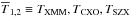${\overline{\mathit{T}}}_{\mathrm{1}\mathit{,}\mathrm{2}}\mathrm{\equiv }{\mathit{T}}_{\mathrm{XMM}}\mathit{,}{\mathit{T}}_{\mathrm{CXO}}\mathit{,}{\mathit{T}}_{\mathrm{SZX}}$), accounting for error bars on both axis. The fit is linear, but the model is not a straight line because of the zero leveldependance on the effective density map (Eq. (10)). To perform the fit, we followed Orear (1982) and defined the following likelihood, L: 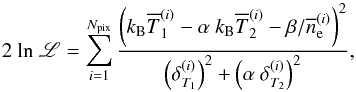$\mathrm{2}\ln L\mathrm{=}\sum _{\mathit{i}\mathrm{=}\mathrm{1}}^{{\mathit{N}}_{\mathrm{pix}}}\frac{{\left({\mathit{k}}_{\mathrm{B}}\overline{\mathit{T}}\begin{array}{c}\mathrm{\left(}\mathit{i}\mathrm{\right)}\\ \mathrm{1}\end{array}\mathrm{-}\mathit{\alpha }{\mathit{k}}_{\mathrm{B}}\overline{\mathit{T}}\begin{array}{c}\mathrm{\left(}\mathit{i}\mathrm{\right)}\\ \mathrm{2}\end{array}\mathrm{-}\mathit{\beta }\mathit{/}\overline{\mathit{n}}\begin{array}{c}\mathrm{\left(}\mathit{i}\mathrm{\right)}\\ \mathrm{e}\end{array}\right)}^{\mathrm{2}}}{{\mathrm{(}{{\mathit{\delta }}_{{\mathit{T}}_{\mathrm{1}}}^{\mathrm{\left(}\mathit{i}\mathrm{\right)}}}^{\mathrm{)}}}^{\mathrm{2}}\mathrm{+}{\mathrm{(}\mathit{\alpha }{{\mathit{\delta }}_{{\mathit{T}}_{\mathrm{2}}}^{\mathrm{\left(}\mathit{i}\mathrm{\right)}}}^{\mathrm{)}}}^{\mathrm{2}}}\mathit{,}$(B.1)where δ_T1,2 represents the temperature map uncertainties, and β is set to zero when the regression is performed between T_XMM and T_CXO. The parameter space was sampled using Markov Chains, which we evolved according to the Metropolis-Hasting algorithm (Chib & Greenberg 1995), as carried out in Adam et al. (2015). We checked that this method correctly reproduced the true posterior likelihood using Monte Carlo realisations (pairs of temperature maps taken as the truth, to which we added a noise realisation as expected from the error estimates). Following (Pratt et al. 2009), we computed the overall scatter as ${\mathit{\sigma }}_{\mathrm{tot}}^{\mathrm{2}}\mathrm{=}\frac{\frac{\mathrm{1}}{{\mathit{N}}_{\mathrm{pix}}\mathrm{-}\mathrm{2}}{\sum }_{\mathit{i}}\frac{{\left({\mathit{k}}_{\mathrm{B}}\overline{\mathit{T}}\begin{array}{c}\mathrm{\left(}\mathit{i}\mathrm{\right)}\\ \mathrm{1}\end{array}\mathrm{-}\mathit{\alpha }{\mathit{k}}_{\mathrm{B}}\overline{\mathit{T}}\begin{array}{c}\mathrm{\left(}\mathit{i}\mathrm{\right)}\\ \mathrm{2}\end{array}\mathrm{-}\mathit{\beta }\mathit{/}\overline{\mathit{n}}\begin{array}{c}\mathrm{\left(}\mathit{i}\mathrm{\right)}\\ \mathrm{e}\end{array}\right)}^{\mathrm{2}}}{{\left({\mathit{\delta }}_{{\mathit{T}}_{\mathrm{1}}}^{\mathrm{\left(}\mathit{i}\mathrm{\right)}}\right)}^{\mathrm{2}}\mathrm{+}{\left(\mathit{\alpha }{\mathit{\delta }}_{{\mathit{T}}_{\mathrm{2}}}^{\mathrm{\left(}\mathit{i}\mathrm{\right)}}\right)}^{\mathrm{2}}}}{\frac{\mathrm{1}}{{\mathit{N}}_{\mathrm{pix}}}{\sum }_{\mathit{i}}\frac{\mathrm{1}}{{\left({\mathit{\delta }}_{{\mathit{T}}_{\mathrm{1}}}^{\mathrm{\left(}\mathit{i}\mathrm{\right)}}\right)}^{\mathrm{2}}\mathrm{+}{\left(\mathit{\alpha }{\mathit{\delta }}_{{\mathit{T}}_{\mathrm{2}}}^{\mathrm{\left(}\mathit{i}\mathrm{\right)}}\right)}^{\mathrm{2}}}}\mathit{,}$(B.2)from which we extracted the intrinsic scatter, ${\mathit{\sigma }}_{\mathrm{int}}\mathrm{=}\sqrt{{\mathit{\sigma }}_{\mathrm{tot}}^{\mathrm{2}}\mathrm{-}{\mathit{\sigma }}_{\mathrm{stat}}^{\mathrm{2}}}$, accounting for the statistical scatter σ_stat.

We also checked that our posterior likelihoods were consistent with the distribution of best-fitting values obtained when fitting independently our 100 Monte Carlo map realisations (T_X and T_SZX; see Appendix A and Sect. 3.4). Nevertheless, we stress that this fitting method does not fully account for the nature of the data themselves. Indeed the recovery of the X-ray spectroscopic temperature maps implies pixel-to-pixel correlations, which depend on the photon count statistics and thus on the sky coordinate and cluster regions. The tSZ signal is also correlated in the NIKA data, but in a different way owing to beam effects, and the noise is spatially correlated. We thus expect that the T_X and T_SZX map pixels do not contain the exact same sky information. These complexities, inherent to the data, are not fully accounted for in our fit. This could lead to small displacements of the best-fit values that we recover and to a slight underestimation of the error contours. However, our baseline pixel size of 20 arcsec allows us to mitigate these effects.

All Tables

All Figures

Fig. 1 Left: effective line of sight electron density, ${\overline{\mathit{n}}}_{\mathrm{e}}$, derived from XMM-Newton. Right: effective line of sight pressure, ${\overline{\mathit{P}}}_{\mathrm{e}}$, derived from NIKA is shown. These maps correspond to model M1, and were smoothed with a Gaussian kernel to an effective resolution of 22 arcsec FWHM. The pressure map is cleaned from our best-fit kSZ model and corrected for the zero level.

In the text

	Fig. 2 Temperature maps. Top: spectroscopic temperature derived from Chandra (TCXO, left panel) and from XMM-Newton (TXMM, right panel) are shown. Bottom: NIKA and XMM-Newton imaging derived temperature, TSZX, for model M1 (left panel) and model M3a (right panel) are shown. These maps are corrected for the zero level.
In the text

	Fig. 3 Correlation between the temperature maps of Fig. 2 and residual. Left: XMM-Newton vs. Chandra spectroscopic temperatures is shown. Middle: tSZ+X-ray imaging (model M1) vs. XMM-Newton spectroscopy is shown. Right: tSZ+X-ray imaging (model M1) vs. Chandra spectroscopy is shown. The red and green dots correspond to the case with and without the kSZ correction, respectively.
In the text

Fig. 4 Posterior likelihood (68 and 95% C.L.) in the plane α – β (expressed in term of the zero level brightness of the NIKA map). Left: tSZ+X-ray imaging vs. XMM-Newton spectroscopy is shown. Right: tSZ+X-ray imaging vs. Chandra spectroscopy is shown. The red and green dots correspond to the case with and without the kSZ correction, respectively, and the different models are provided with different dashed line as shown in the legend.

In the text

References

- Adam, R., Comis, B., Macías-Pérez, J. F., et al. 2014, A&A, 569, A66 [NASA ADS] [CrossRef] [EDP Sciences] [Google Scholar]
- Adam, R., Comis, B., Macías-Pérez, J.-F., et al. 2015, A&A, 576, A12 [NASA ADS] [CrossRef] [EDP Sciences] [Google Scholar]
- Adam, R., Comis, B., Bartalucci, I., et al. 2016, A&A, 586, A122 [NASA ADS] [CrossRef] [EDP Sciences] [Google Scholar]
- Adam, R., Bartalucci, I., Pratt, G. W., et al. 2017, A&A, 598, A115 [NASA ADS] [CrossRef] [EDP Sciences] [Google Scholar]
- Allen, S. W., Evrard, A. E., & Mantz, A. B. 2011, ARA&A, 49, 409 [NASA ADS] [CrossRef] [Google Scholar]
- Basu, K., Zhang, Y.-Y., Sommer, M. W., et al. 2010, A&A, 519, A29 [NASA ADS] [CrossRef] [EDP Sciences] [Google Scholar]
- Bourdin, H., & Mazzotta, P. 2008, A&A, 479, 307 [NASA ADS] [CrossRef] [EDP Sciences] [Google Scholar]
- Calvo, M., Roesch, M., Désert, F.-X., et al. 2013, A&A, 551, L12 [NASA ADS] [CrossRef] [EDP Sciences] [Google Scholar]
- Calvo, M., Benoît, A., Catalano, A., et al. 2016, J. Low Temp. Phys., 184, 816 [NASA ADS] [CrossRef] [Google Scholar]
- Catalano, A., Calvo, M., Ponthieu, N., et al. 2014, A&A, 569, A9 [NASA ADS] [CrossRef] [EDP Sciences] [Google Scholar]
- Chib, S., & Greenberg, E. 1995, The American Statistician, 49, 327 [Google Scholar]
- Comis, B., Adam, R., Ade, P., et al. 2016, ArXiv e-prints [arXiv:1605.09549] [Google Scholar]
- Croston, J. H., Arnaud, M., Pointecouteau, E., & Pratt, G. W. 2006, A&A, 459, 1007 [NASA ADS] [CrossRef] [EDP Sciences] [Google Scholar]
- Dicker, S. R., Ade, P. A. R., Aguirre, J., et al. 2014, in Millimeter, Submillimeter, and Far-Infrared Detectors and Instrumentation for Astronomy VII, Proc. SPIE, 9153, 91530J [NASA ADS] [CrossRef] [Google Scholar]
- Eckert, D., Molendi, S., Vazza, F., Ettori, S., & Paltani, S. 2013, A&A, 551, A22 [NASA ADS] [CrossRef] [EDP Sciences] [Google Scholar]
- Itoh, N., & Nozawa, S. 2003, ArXiv e-prints [arXiv:astro-ph/0307519] [Google Scholar]
- Khedekar, S., Churazov, E., Kravtsov, A., et al. 2013, MNRAS, 431, 954 [NASA ADS] [CrossRef] [Google Scholar]
- Kitayama, T., Komatsu, E., Ota, N., et al. 2004, PASJ, 56, 17 [NASA ADS] [Google Scholar]
- Ma, C.-J., Ebeling, H., & Barrett, E. 2009, ApJ, 693, L56 [NASA ADS] [CrossRef] [Google Scholar]
- Mahdavi, A., Hoekstra, H., Babul, A., et al. 2013, ApJ, 767, 116 [NASA ADS] [CrossRef] [Google Scholar]
- Markevitch, M., & Vikhlinin, A. 2007, Phys. Rep., 443, 1 [NASA ADS] [CrossRef] [EDP Sciences] [Google Scholar]
- Mathiesen, B. F., & Evrard, A. E. 2001, ApJ, 546, 100 [CrossRef] [Google Scholar]
- Mazzotta, P., Rasia, E., Moscardini, L., & Tormen, G. 2004, MNRAS, 354, 10 [NASA ADS] [CrossRef] [Google Scholar]
- Monfardini, A., Benoit, A., Bideaud, A., et al. 2011, ApJS, 194, 24 [NASA ADS] [CrossRef] [Google Scholar]
- Mroczkowski, T., Dicker, S., Sayers, J., et al. 2012, ApJ, 761, 47 [NASA ADS] [CrossRef] [Google Scholar]
- Nagai, D., & Lau, E. T. 2011, ApJ, 731, L10 [NASA ADS] [CrossRef] [Google Scholar]
- Nagai, D., Vikhlinin, A., & Kravtsov, A. V. 2007, ApJ, 655, 98 [NASA ADS] [CrossRef] [Google Scholar]
- Nord, M., Basu, K., Pacaud, F., et al. 2009, A&A, 506, 623 [NASA ADS] [CrossRef] [EDP Sciences] [Google Scholar]
- Orear, J. 1982, Amer. J. Phys., 50, 912 [NASA ADS] [CrossRef] [EDP Sciences] [Google Scholar]
- Planck Collaboration I. 2016, A&A, 594, A1 [NASA ADS] [CrossRef] [EDP Sciences] [Google Scholar]
- Planck Collaboration XIII. 2016, A&A, 594, A13 [NASA ADS] [CrossRef] [EDP Sciences] [Google Scholar]
- Pointecouteau, E., Giard, M., & Barret, D. 1998, A&A, 336, 44 [NASA ADS] [Google Scholar]
- Pointecouteau, E., Hattori, M., Neumann, D., et al. 2002, A&A, 387, 56 [NASA ADS] [CrossRef] [EDP Sciences] [Google Scholar]
- Pratt, G. W., Croston, J. H., Arnaud, M., & Böhringer, H. 2009, A&A, 498, 361 [NASA ADS] [CrossRef] [EDP Sciences] [Google Scholar]
- Rasia, E., Lau, E. T., Borgani, S., et al. 2014, ApJ, 791, 96 [NASA ADS] [CrossRef] [Google Scholar]
- Ruppin, F., Adam, R., Comis, B., et al. 2017, A&A, 597, A110 [NASA ADS] [CrossRef] [EDP Sciences] [Google Scholar]
- Sarazin, C. L. 1988, X-ray emission from clusters of galaxies (Cambridge: Cambridge University Press) [Google Scholar]
- Sayers, J., Mroczkowski, T., Zemcov, M., et al. 2013, ApJ, 778, 52 [NASA ADS] [CrossRef] [Google Scholar]
- Schellenberger, G., Reiprich, T. H., Lovisari, L., Nevalainen, J., & David, L. 2015, A&A, 575, A30 [NASA ADS] [CrossRef] [EDP Sciences] [Google Scholar]
- Sunyaev, R. A., & Zeldovich, I. B. 1980, MNRAS, 190, 413 [NASA ADS] [CrossRef] [Google Scholar]
- Sunyaev, R. A., & Zeldovich, Y. B. 1972, Comm. Astrophys. Space Phys., 4, 173 [Google Scholar]
- Tchernin, C., Eckert, D., Ettori, S., et al. 2016, A&A, 595, A42 [NASA ADS] [CrossRef] [EDP Sciences] [Google Scholar]
- Vazza, F., Eckert, D., Simionescu, A., Brüggen, M., & Ettori, S. 2013, MNRAS, 429, 799 [NASA ADS] [CrossRef] [Google Scholar]
- Vikhlinin, A. 2006, ApJ, 640, 710 [NASA ADS] [CrossRef] [Google Scholar]
- Zhuravleva, I., Churazov, E., Kravtsov, A., et al. 2013, MNRAS, 428, 3274 [NASA ADS] [CrossRef] [Google Scholar]