| Issue |
A&A
Volume 605, September 2017
|
|
|---|---|---|
| Article Number | A58 | |
| Number of page(s) | 21 | |
| Section | Interstellar and circumstellar matter | |
| DOI | https://doi.org/10.1051/0004-6361/201731019 | |
| Published online | 08 September 2017 | |
Galactic supernova remnant candidates discovered by THOR
1 Department of Physics and Astronomy, West Virginia University, Morgantown, WV 26506, USA
e-mail: This email address is being protected from spambots. You need JavaScript enabled to view it.
2 Adjunct Astronomer at the Green Bank Observatory, PO Box 2, Green Bank, WV 24944, USA
3 Center for Gravitational Waves and Cosmology, West Virginia University, Chestnut Ridge Research Building, Morgantown, WV 26505, USA
4 Max Planck Institute for Astronomy, Königstuhl 17, 69117 Heidelberg, Germany
5 Universität Heidelberg, Zentrum für Astronomie, Institut für Theoretische Astrophysik, Albert-Ueberle-Str. 2, 69120 Heidelberg, Germany
6 Harvard-Smithsonian Center for Astrophysics, Cambridge, MA 02138, USA
7 Department of Astronomy, University of Wisconsin-Madison, 475 N. Charter street, Madison, WI 53706, USA
8 Department of Astronomy, University of Massachusetts, Amherst, MA 01003-9305, USA
9 Astrophysics Research Institute, Liverpool John Moores University, 146 Brownlow Hill, Liverpool L3 5RF, UK
10 Max Planck Institute for Radioastronomy, Auf dem Hügel 69, 53121 Bonn, Germany
11 National Radio Astronomy Observatory, PO Box O, 1003 Lopezville Road, Socorro, NM 87801, USA
12 Department of Physics, Indian Institute of Science, 560012 Bangalore, India
13 Department of Physics and Astronomy, University of Calgary, 2500 University Drive NW, Calgary AB, T2N 1N4, Canada
14 School of Physical Sciences, University of Kent, Ingram Building, Canterbury, Kent CT2 7NH, UK
Received: 20 April 2017
Accepted: 28 May 2017
Abstract
Context. There is a considerable deficiency in the number of known supernova remnants (SNRs) in the Galaxy compared to that expected. This deficiency is thought to be caused by a lack of sensitive radio continuum data. Searches for extended low-surface brightness radio sources may find new Galactic SNRs, but confusion with the much larger population of H ii regions makes identifying such features challenging. SNRs can, however, be separated from H ii regions using their significantly lower mid-infrared (MIR) to radio continuum intensity ratios.
Aims. Our goal is to find missing SNR candidates in the Galactic disk by locating extended radio continuum sources that lack MIR counterparts.
Methods. We use the combination of high-resolution 1–2 GHz continuum data from The HI, OH, Recombination line survey of the Milky Way (THOR) and lower-resolution VLA 1.4 GHz Galactic Plane Survey (VGPS) continuum data, together with MIR data from the Spitzer GLIMPSE, Spitzer MIPSGAL, and WISE surveys to identify SNR candidates. To ensure that the candidates are not being confused with H ii regions, we exclude radio continuum sources from the WISE Catalog of Galactic H ii Regions, which contains all known and candidate H ii regions in the Galaxy.
Results. We locate 76 new Galactic SNR candidates in the THOR and VGPS combined survey area of 67.4° > ℓ > 17.5°, | b | ≤ 1.25° and measure the radio flux density for 52 previously-known SNRs. The candidate SNRs have a similar spatial distribution to the known SNRs, although we note a large number of new candidates near ℓ ≃ 30°, the tangent point of the Scutum spiral arm. The candidates are on average smaller in angle compared to the known regions, 6.4′ ± 4.7′ versus 11.0′ ± 7.8′, and have lower integrated flux densities.
Conclusions. The THOR survey shows that sensitive radio continuum data can discover a large number of SNR candidates, and that these candidates can be efficiently identified using the combination of radio and MIR data. If the 76 candidates are confirmed as true SNRs, for example using radio polarization measurements or by deriving radio spectral indices, this would more than double the number of known Galactic SNRs in the survey area. This large increase would still, however, leave a discrepancy between the known and expected SNR populations of about a factor of two.
Key words: Hiiregions / ISM: supernova remnants / radio continuum: ISM / infrared: ISM
© ESO, 2017
1. Introduction
There is a severe discrepancy in the number of detected supernova remnants (SNRs) in the Galaxy compared to that expected. The most authoritative recent compilation contains just 294 SNRs (Green 2014, hereafter G14), but based on OB star counts, pulsar birth rates, Fe abundances, and the SN rate in other Local Group galaxies, there should be ≳ 1000 (Li et al. 1991; Tammann et al. 1994). These estimates derive in part from studies of similar external galaxies, scaled to the Milky Way based on its luminosity. The discrepancy may not be due to a true deficiency of Galactic SNRs, but rather may hint at observational problems related to lack of sensitivity and confusion in the Galactic plane (e.g., Brogan et al. 2006, hereafter B06).
The Galactic supernova (SN) rate is an important parameter for understanding the properties and dynamics of our Galaxy. Most SN arise from the core collapse of massive stars (cf. Tammann et al. 1994), and therefore the number of SNRs in the Galaxy is tied to recent massive star formation activity. SN inject energy into the interstellar medium (ISM), driving molecular cloud turbulence and galactic fountains out of the disk (de Avillez & Breitschwerdt 2005; Joung et al. 2009; Padoan et al. 2016; Girichidis et al. 2016). This feedback can determine the disk scale height and star formation properties of a galaxy (Ostriker et al. 2010; Ostriker & Shetty 2011; Faucher-Giguère et al. 2013). The search for new Galactic SNRs is therefore important for understanding the global properties of the Milky Way.
SNRs are frequently identified at radio wavelengths. According to the G14 catalog, ~ 90% of known SNRs are detected and well-defined in the radio regime, ~ 40% detected in X-rays, and ~ 30% in the optical. The radio emission is due to synchrotron radiation, which dominates the Galaxy’s low-frequency radio emission. The most common radio morphology in the G14 catalog is that of a shell, or a partial shell.
Since many types of objects emit radio emission similar to that of known SNRs, additional criteria are used to determine if a radio continuum source is a true SNR. These criteria are: 1) the radio spectrum of candidate has a negative spectral index (typically ~−0.5); 2) the radio emission from the candidate is polarized; 3) the candidate has associated X-ray or cosmic ray emission; and/or 4) the candidate has a mid-infrared (MIR) to radio continuum flux ratio much lower than that commonly found for thermally-emitting plasmas. The first two criteria can distinguish between thermal (flat spectrum, unpolarized) and non-thermal (negative spectral index, polarized) radio emission. The third criterion is sensitive to high-temperature (~ 107 K) plasma within SNRs that is rarely detected in H ii regions. The fourth criterion has characteristics of the other three, in that it can also distinguish between thermal and non-thermal emitters. The MIR emission from dust arises from the interaction of the SN shock wave with the ISM during the initial expansion phases (e.g., Douvion et al. 2001). Other non-thermal radio continuum sources such as active galactic nuclei can be excluded from SNR searches due to their small angular sizes.
Many researchers have shown that SNRs are deficient in MIR emission compared to H ii regions (e.g., Cohen & Green 2001; Pinheiro Gonçalves et al. 2011). For SNRs to produce MIR emission, they must be sufficiently dense to produce collisional heating (Williams et al. 2006). Pinheiro Gonçalves et al. (2011) found that a typical 24 μm to 1.4 GHz flux density ratio for SNRs is ~ 5, although they found flux density ratios ranging from 0.5 to 10. This low MIR to radio flux ratio holds even for young regions like Cas A, despite their strong MIR emission (see Rho et al. 2008). Due to its powerful discriminatory power and relative ease of use, the MIR to radio flux ratio is of most interest here.
SNR candidates can be identified efficiently in radio continuum surveys using their low MIR to radio continuum flux ratios. While there is some faint associated MIR emission detected for some SNRs (Reach et al. 2006; Pinheiro Gonçalves et al. 2011), this emission is quite weak. At radio frequencies high enough that H ii regions are optically thin, ≳ 1 GHz, the MIR to radio flux ratio for SNRs is about 100 times lower than that of H ii regions. Helfand et al. (2006, hereafter H06), used the lack of MIR emission as one criterion to identify 49 new SNR candidates in The Multi-Array Galactic Plane Imaging Survey (MAGPIS) 20 cm data. B06 also used this criterion to identify 35 SNR candidates in their VLA data. Recently, Green et al. (2014) used the anti-correlation between radio and 8 μm emission to identify 23 new SNR candidates from Molonglo Galactic Plane Survey (MGPS) data.
These previous studies have first identified promising radio continuum candidates, and then examined their 8.0 μm emission to determine their classifications. This method, however, has an inherent bias toward objects that look like SNRs, i.e. shell-type structures, at the expense of other possible SNR morphologies. A better method is to first identify all H ii regions from their MIR morphologies and high MIR to radio continuum flux density ratios, and to then locate radio continuum sources not associated with the H ii regions. This removes the confusion from H ii regions in the Galactic plane, which is a major difficulty in new SNR identifications given their potentially similar radio morphologies and the much higher spatial density of H ii regions. By excluding H ii regions, one can search for non-thermal emission features without imposing any source morphology bias.
Here, we identify extended sources of emission in radio continuum data from The H I, OH, Recombination line survey of the Milky Way (THOR; Beuther et al. 2016) combined with the 1.4 GHz radio continuum data from the VLA Galactic Plane Survey (VGPS Stil et al. 2006). In the identification process, we first use the WISE Catalog of Galactic H ii Regions (Anderson et al. 2014) to separate thermal and non-thermal extended emission. Compact sources of radio continuum emission detected by THOR are analyzed in Bihr et al. (2016) and Wang et al. (in prep.). We focus instead on diffuse, resolved sources that are “discrete”, i.e. distinct from the diffuse background emission that pervades the Galactic disk.
2. Data
2.1. THOR
THOR is a ~ 20 cm VLA survey of H I, OH, radio recombination line, and radio continuum emission in the Galactic plane from 67.4°>ℓ> 14.5°, | b | ≤ 1.25°. It was conducted in VLA C-configuration, with a resolution of ~ 20″. More survey details are given in Beuther et al. (2016). When the THOR continuum data are combined with 20 cm VGPS continuum data, taken with the VLA in D-configuration at a resolution of 60″ and data taken with the 100 m Effelsberg telescope at a resolution of 9′, the resulting data product is the most sensitive radio continuum Galactic plane survey in existence covering both large and small spatial scales. We call this combined data set “THOR+VGPS”. The THOR+VGPS data have an angular resolution of 25″ because of smoothing we apply to the THOR data (see Beuther et al. 2016). Due to the coverage of the VGPS, the THOR+VGPS data set is restricted to ℓ> 17.5°, so our final longitude range is 67.4°>ℓ> 17.5°.
To detect low surface brightness SNRs, the radio observations must be sensitive to large, extended structures. To reduce confusion in the Galactic plane, the data should also have high angular resolution. The sensitivity of the THOR+VGPS data changes slightly over the extent of the survey, but a typical 1σ rms value is ~ 1 mJy beam-1 (Bihr et al. 2016), or ~ 1 × 10-22 W m-2 Hz-1 sr-1. Over scales greater than that of the VGPS VLA D-configuration data (~ 15′), the surface brightness sensitivity should approach that of the Effelsberg single-dish data used in the VGPS, ~ 1 × 10-23 W m-2 Hz-1 sr-1 (Reich & Reich 1986; Reich et al. 1990), although the VLA data do add some noise on large spatial scales. The low surface brightness noise threshold, together with the sensitivity to small-scale structures, makes the THOR survey the ideal data set to identify new SNRs.
2.2. The WISE Catalog of Galactic H II regions
The WISE Catalog of Galactic H ii regions (Anderson et al. 2014) is to date the largest, most complete catalog of H ii regions spanning the entire Galaxy. It was created by searching WISE (Wright et al. 2010) data by-eye for the characteristic MIR signature of H ii regions: ~ 20 μm emission surrounded by ~ 10 μm emission (Anderson et al. 2011). The ~ 20 μm emission is caused by small stochastically heated dust grains that are mixed with the H ii region plasma, while the ~ 10 μm intensity is dominated by emission from polycyclic aromatic hydrocarbons (PAHs). All known Galactic H II regions have this characteristic morphology. Planetary nebulae can appear similar, but they are distinguished by their small sizes and weak far-infrared fluxes (Anderson et al. 2012). The H ii region MIR emission detected by WISE and Spitzer is about two orders of magnitude more intense than the ~ 20 cm radio continuum emission, and these observatories have sensitivities far lower than that necessary to detect H ii regions across the entire Galactic disk (Anderson et al. 2011, 2014). This single MIR morphological criterion can therefore be used to identify all Galactic H ii regions.
The WISE catalog contains ~ 8000 objects with the MIR morphology of H ii regions, of which ~ 2000 are H ii regions with measured ionized gas velocities (Hα or radio recombination line, RRL). This includes all known H ii regions, indicating that the MIR morphological criterion can be used to identify all known Galactic H ii regions. The remaining ~ 6000 sources that lack ionized gas spectroscopic detections are H ii region candidates, and there are two sub-classes: ~ 2000 “radio-loud” candidates that have spatially coincident radio continuum emission and ~ 4000 “radio-quiet” candidates that do not. Radio continuum emission, caused by the free-free emission of the ionized gas, makes the identification of H ii regions more secure (e.g., Haslam & Osborne 1987). The distribution of known regions in the catalog is statistically complete for all H ii regions with ionizing fluxes consistent with single O-stars of all spectral sub-types (Armentrout et al., in prep.; Mascoop et al., in prep.).
2.3. Green catalog
G14 is the most up-to-date and authoritative catalog of Galactic SNRs. It currently contains 294 regions compiled from the literature, and tabulates their spatial coordinates, their 1 GHz flux densities, spectral indices, and angular sizes. The catalog sources cover the entire sky, but since it is not derived from a homogeneous survey, the catalog sensitivity varies with Galactic location. Green (2004) suggest that an earlier version of the catalog than that used here was complete to a radio surface density limit of 10-20 W m-2 Hz-1 sr-1. In addition to the surface brightness limit, the catalog appears to be lacking the small angular size SNRs that are expected (Green 2015).
3. Methodology
Our method relies on identifying discrete regions of radio continuum emission that a) are not associated with H ii regions from the WISE catalog and b) lack Spitzer or WISE MIR emission. These criteria are somewhat redundant, as nearly all discrete sources of coincident MIR and radio continuum emission in the Galactic plane are H ii regions and are included in the WISE catalog. We do not have a preferred morphology for the regions we identify aside for avoiding long filamentary radio continuum features that, based on the morphologies of known SNRs, are not likely to be SNRs.
To locate new SNR candidates, we search the THOR+VGPS data by-eye. We first identify all discrete, extended radio continuum sources that are not associated with an H ii region in the WISE catalog. This initial search allows us to separate SNR candidates from the much more numerous population of H ii regions. We then search Spitzer GLIMPSE 8.0 μm (Benjamin et al. 2003; Churchwell et al. 2009) and MIPSGAL 24 μm (Carey et al. 2009) data at the location of each identified source to ensure that there is no detectable MIR emission. These MIR surveys have sensitivities sufficient to detect all H ii regions across the entire Galaxy. For the few sources with latitudes outside the range of the Spitzer surveys, we use WISE 12 and 22 μm data (Wright et al. 2010). Our process should remove planetary nebulae and any remaining H ii regions not included in the WISE catalog. The remaining radio continuum sources are either SNR candidates or known SNRs. By matching the positions and sizes with the G14 catalog, we determine which of these sources have been previously identified as SNRs. We illustrate the identification process in Fig. 1.
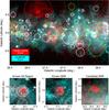 |
Fig. 1 (Top) Two-color images with GLIMPSE 8.0 μm data in cyan and THOR+VGPS 21 cm continuum data in red. H ii regions have 8.0 μm emission surrounding the 21 cm emission. Although not shown, MIPSGAL 24 μm emission has a similar morphology as the radio continuum for H ii regions, and is essentially absent for SNRs. The candidate SNRs are enclosed by green circles, known SNRs by red circles, and known or candidate H ii regions by white circles. Dotted boxes enclose the areas displayed as insets below. These insets show a known H ii region that has bright 8.0 μm emission (left; G028.022−00.043), a known SNR (middle; G27.4+0.0), and an example SNR candidate (right; G26.75+0.73). The H ii region has strong 8.0 μm emission surrounding the radio continuum, but the known and candidate SNRs are devoid of 8.0 μm emission. |
For each identified SNR candidate, as well as all previously-known SNRs, we compute the 1.4 GHz THOR+VGPS flux density using aperture photometry, following the methodology of Anderson et al. (2012). We define a circular aperture for each source that completely contains its radio continuum emission. For SNR candidates that have partial-shell morphologies, the circular aperture follows the curvature of the visible portion of the shell. We define four background apertures for each source. The background apertures sample the local background and avoid discrete continuum sources not associated with the SNR. We attempt to make the background apertures as large as possible, and to space them evenly around the source. If there are large-scale gradients in the background level, however, we sample these gradients. In complicated fields, we must define smaller background apertures, but we still aim to space them evenly around the source. Five SNR candidates are low surface brightness and confused with nearby regions, and we do not compute their flux densities.
THOR SNR candidates.
We then compute the source integrated intensity as 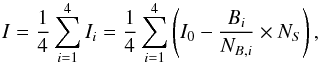 (1)and the source integrated intensity uncertainty as
 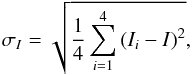 (2)where the summations are carried out over the four background apertures, I is the average integrated source intensity, Ii is the integrated source intensity found using one background aperture, I0 is integrated source intensity before background subtraction, Bi is the integrated intensity from one background aperture, NB,i is the number of pixels within one background aperture, and NS is the number of pixels within the source aperture. This method subtracts the mean intensity of a background aperture from every pixel in the source aperture. The derived uncertainties ignore the approximately 20% uncertainty in the absolute intensity calibration of the THOR+VGPS data.
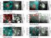 |
Fig. 2 Example images for select SNR candidates, showing the range of surface brightnesses and morphologies. The left panels show two-color GLIMPSE 8.0 μm (cyan) and THOR+VGPS 21 cm (red), as in Fig. 1. The right panels show THOR+VGPS data alone. Circles in both panels are the same as in Fig. 1, with candidate SNRs are enclosed by green circles, known SNRs by red circles, and known or candidate H ii regions by white circles. |
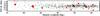 |
Fig. 3 Galactic distribution of the new candidate (green) and known (red) SNRs. The circles approximate the SNR sizes, but due to the aspect ratio of the plot, the sizes are only valid along the Galactic longitude axis. The background is a two-dimensional histogram of the H ii region density, with higher densities indicated by darker colors. |
We convert I, which has units of Jy beam-1, to flux densities in Jy using the THOR+VGPS circular synthesized beam size of 25″. If there are any unrelated continuum sources that fall within the source aperture (typically extragalactic point sources or H ii regions), we manually remove their flux densities from the source flux density. We use only the flux density values, rather than intensities, in subsequent analyses.
There are a couple complications with our method. First, there are numerous filamentary features in the Galactic plane observed in radio continuum emission. These features are frequently located near large massive star formation complexes. We interpret them as being dense thermally emitting ionized gas interacting with atomic or molecular material in the ISM, and do not catalog such regions as possible SNRs. Another unrelated complication also arises around massive star formation complexes, where bright continuum emission produces interferometric artifacts that do not have MIR counterparts, and therefore can be mistaken for SNRs (see Beuther et al. 2016, their Figs. 7 and 8). To reduce the chance of identifying artifacts, we verify that all identified SNR candidates near large star formation complexes are also detected in the NVSS (Condon et al. 1998) or MAGPIS surveys. Due to the higher probability that a radio continuum feature is thermally emitting ionized gas or an interferometric artifact, we are conservative in our identifications around large star formation complexes.
We classify the radio continuum morphology of each SNR candidate as “shell”, for those with well-defined radio continuum shells, “filled”, for those lacking an outer shell but emission filling a roughly circular region, or “composite” for those that have a shell with a filled interior. For seven of the smallest regions, the THOR+VGPS resolution is insufficient to determine their morphological classification.
4. Results
We identify 76 new Galactic SNR candidates, and detect the radio continuum emission from 52 of 53 previously-known SNRs from the G14 catalog. In our aperture photometry measurements, we create a circular aperture that encloses the radio continuum emission of each source and therefore define the centroid and radius of each region. We give parameters of the new SNR candidates in Table 1, which lists the Galactic longitude, Galactic latitude, and radius, as defined in THOR+VGPS data, the 1.4 GHz THOR+VGPS flux density and its uncertainty, and the radio continuum morphological type, and the name from H06 if the same source was identified there. Seven SNR candidates are so confused with nearby radio continuum sources that their flux densities are unreliable; we do not list flux densities for these seven regions. We give the parameters of the G14 regions in Table 2, which has the same columns as Table 1 but additionally contains the 1 GHz flux density and spectral index (α) from the G14 catalog. We show THOR+VGPS and MIR two-color images for example SNR candidates in Fig. 2, and for all candidates in the Appendix. We plot the Galactic locations of all known and candidate SNRs in Fig. 3.
4.1. New SNR candidates
All 76 SNR candidates have THOR+VGPS 21 cm continuum emission and a deficiency of MIR emission compared with H ii regions. Of the 76 candidates, seven were identified previously as being possible SNRs in H06, and one was identified in B06. These works utilized the same MIR deficit as we use here, but also employed data from multiple radio frequencies in an effort to determine the spectral indices. Our identifications therefore provide some additional support to the object being a true SNR, although this support is limited due to the similarities between our methodologies.
THOR includes multiple continuum spectral windows that in principle allow for the computation of spectral indices. Because the VGPS data only have one continuum spectral window, however, we cannot compute spectral indices for SNR candidates that require THOR+VGPS data to be detected. Bihr et al. (2016) did detect compact emission toward several smaller SNR candidates in individual THOR spectral windows in the first half of the THOR survey, and several more were detected in the second half of the survey (Wang et al., in prep.). All candidates detected in THOR data alone have negative spectral indices consistent with them being true SNRs.
G14 known SNRs.
4.2. G14 SNRs
We confirm the radio emission for 52 G14 SNRs that lie within the THOR+VGPS zone, but we did not detect THOR+VGPS radio emission from G66.0−0.0. This region was detected in radio continuum emission by Sabin et al. (2013) in the GB6 5 GHz data (Gregory et al. 1996). They note that it was not detected at 20 cm, which we confirm in the THOR+VGPS data. The nature of this source is therefore unclear.
The flux densities derived from our aperture photometry measurements agree well with those listed in the G14 catalog, as illustrated by Fig. 4. The G14 catalog contains flux densities at 1 GHz, extrapolated from the values measured using the derived spectral index, but does not contain flux density uncertainties. Some 1 GHz flux densities are marked as being uncertain in the G14 catalog, and these have especially large discrepancies with the THOR+VGPS values. That the relationship is so close to 1:1 is evidence that the THOR+VGPS data are well-calibrated relative to previous measurements in the literature.
Six G14 SNRs appear to be confused with H ii regions: G20.4+0.1, G21.5−0.1, G23.6+0.3, G54.1+0.3, G59.8+1.2 and G065.8−0.5. We show THOR+VGPS data, as well as GLIMPSE 8.0 μm or WISE 12 μm data, for these regions in Fig. 5. These two infrared data sets exhibit the same morphology for H ii regions (Anderson et al. 2012). We use the WISE data only if the GLIMPSE coverage is not sufficient. We discuss the individual regions below.
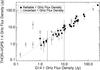 |
Fig. 4 THOR+VGPS 1.4 GHz flux densities compared with G14 1 GHz flux densities. Filled circles denote SNRs that have more secure values in the G14 catalog, whereas open circles are more uncertain (values that have a question mark in the G14 catalog). The dotted line shows a 1:1 relationship. |
G20.4+0.1:
the spectral index for G20.4+0.1 was found by B06 to be −0.4, but a value of −0.08 ± 0.09 was derived by Sun et al. (2011). Additionally, Pinheiro Gonçalves et al. (2011) measured a high MIR to radio flux ratio consistent with that of H ii regions. It is spatially coincident with WISE H ii region G020.482+00.167, which has measured RRL emission from Lockman (1989), providing further evidence that the radio emission is thermal. The radio continuum emission extends to the west of the identified H ii region enclosed by 8.0 μm emission. Based on its association with MIR emission, this western extension appears to also be thermal, possibly resulting from photons leaking from the H ii region (see Luisi et al. 2016).
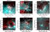 |
Fig. 5 G14 SNRs confused with H ii regions. Shown for each region are two-color images with GLIMPSE 8.0 μm (for G20.4+0.1, G21.5−0.1, G23.6+0.3, and G54.1+0.3) or WISE 12 μm data (for G59.8+1.2 and G65.8−0.5) in cyan and THOR+VGPS 21 cm continuum data in red. The central positions are taken from the G14 catalog, and the image dimensions are three times the G14 SNR diameters. As in Fig. 1, the candidate SNRs are enclosed by green circles and known or candidate H ii regions by white circles. Red dotted circles show the expected position and size of the G14 SNRs that are confused with H ii regions. |
G21.5−0.1:
the radio emission of G21.5−0.1 is entirely spatially coincident with the WISE H ii region G021.560−00.108, and is bordered by GLIMPSE 8.0 μm emission. The H ii region has measured RRL emission (Anderson et al. 2015), which suggests that the radio continuum emission is thermal. Its morphology and the high MIR flux further point to this being an H ii region. Using MIPSGAL 24 μm data, Pinheiro Gonçalves et al. (2011) also found a high MIR to radio flux ratio for this region consistent with that of H ii regions.
G23.6+0.3:
this source has radio emission along a bright linear feature. This feature is inside the GLIMPSE 8.0 μm emission, again indicating that the region is an H ii region. This defines a portion of the shell of the WISE H ii region G23.689+00.377, which has measured RRL emission (Lockman et al. 1996). Similar to G21.5−0.1, Pinheiro Gonçalves et al. (2011) found a high MIR to radio ratio for G21.5−0.1. On this basis they suggested that is an H ii region.
G54.1+0.3:
Lang et al. (2010) noted that the extended radio emission in the field of G54.1+0.3 is ambiguous: it could be non-thermal emission associated with the pulsar wind nebula G54.1+0.3 (the compact object at the center of the image shown in Fig. 5) or could be thermal emission. They further note that 24 μm MIPSGAL emission has a similar morphology as the radio loop, hinting that it may be thermal emission. We support the latter interpretation, and associate the radio continuum emission with the WISE H ii region G053.935+00.228. On its western edge there is strong 8.0 μm GLIMPSE emission, and the radio emission is found interior to this MIR emission. Lockman (1989) measured RRL emission from a position on the western edge. Together, these data indicate that the radio emission previously suggested as being a possible SNR remnant associated with the G54.1+0.3 pulsar wind nebula (PWN) actually represents a thermal H ii region. Importantly, however, there is diffuse, extended radio emission that has a different morphology from the ring structure. This emission is faint, centered approximately on the compact PWN, and has a radius of 5′. We include it as a candidate SNR.
G59.8+1.2:
although G59.8+1.2 is almost certainly an H ii region, there is a nearby patch of radio emission that, based on its lack of MIR emission, does appear to be nonthermal. We identify this non-thermal emission as SNR candidate G59.68+1.25. These two regions are perhaps confused in the literature. We suggest that the G59.8+1.2 object is actually the WISE H ii region G059.803+01.228, which has measured RRL emission (Anderson et al., in prep.). The region was also listed as having a flat spectral index by Sun et al. (2011), who additionally note that more observations are required to establish its classification, in support of it being confused with the nearby H ii regions.
G65.8−0.5:
the case of G65.8−0.5 is especially confusing. Much of the H-α emission mentioned in Sabin et al. (2013) is associated with the compact WISE H ii region candidate G065.887−00.605. This region is a candidate because although it has the characteristic MIR and radio continuum morphology of H ii regions, it has not been measured in RRL or H-α spectroscopic observations. Sabin et al. (2013) show low-frequency radio data with a slightly extended morphology not present in the THOR+VGPS data. Given that the low-frequency radio data peak intensity is spatially coincident with the H ii region, it seems likely that all the radio emission is thermal.
4.3. H06 and B06 mis-identifications
Many SNR candidates identified in the MAGPIS survey of H06 are actually H ii regions. Additionally, we suggest that one B06 SNR candidate (G19.13+0.90) is a thermally-emitting filament. We show the mis-identified MAGPIS regions, as well as G19.13+0.90, in Fig. 6.
The 17 mis-identified MAGPIS SNR candidates are: G18.2536–0.3083, G19.4611+0.1444, G19.5800–0.2400, G19.5917+0.0250, G19.6100–0.1200, G19.6600–0.2200, G21.6417+0.0000, G22.7583–0.49171, G22.9917–0.3583, G23.5667–0.0333, G24.1803+0.2167, G25.2222+0.2917, G29.0667–0.6750, G30.8486+0.1333, G31.0583+0.4833, G31.6097+0.3347, and G31.8208–0.1222. All are spatially coincident with a known H ii region from the WISE catalog. Of these, G18.254-0.308 was previously mentioned in Bihr et al. (2016) as being an H ii region. One additional MAGPIS SNR (G29.0778+0.4542) is a known planetary nebula (PN A66 48).
The source G19.13+0.90 from B06 does not appear to be a true SNR. B06 classify this object as “class III”, their lowest certainty of actually being a SNR. It has associated MIR emission, and its radio morphology is that of a long filament. Although it does have a spectral index of −0.5 reported in B06, the morphology and MIR emission from this feature makes its classification as a SNR uncertain.
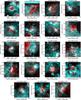 |
Fig. 6 Mis-identified SNR candidates from H06 and B06. The format for these images is the same as that of Fig. 1, with GLIMPSE 8.0 μm data in cyan and THOR+VGPS 21 cm continuum data in red. As in Fig. 1, the candidate SNRs are enclosed by green circles, known SNRs by red circles, and known or candidate H ii regions by white circles. Red dotted circles show the expected position and size of the SNR candidates. All except for G19.1+0.9, which appears to be a radio continuum filament, and G29.0778+0.4542, which is a planetary nebula, are confused with H ii regions. |
4.4. Comparison with known SNRs and H II regions
The Galactic longitude distribution of the SNR candidates shown in the left panel of Fig. 7 is similar to that of the previously known sample. There are, however, larger numbers of candidate SNRs near ℓ ≃ 30° compared with the G14 population. The long bar ends at ℓ ≃ 30° (Benjamin et al. 2005), and the giant H ii region W43 is at this longitude. There is also a greater number of star formation regions at ℓ ≃ 30°, as seen in the WISE H ii region distribution in Figs. 3 and 7. The increased number of SNRs here is consistent with the large star formation rate of the W43 region. Kolmogorov-Smirnov (K-S) tests show that the candidate SNR, G14 SNR, and H ii region populations are consistent with originating from the same parent distribution. We use a K-S probability threshold of 0.01 for this and all subsequent calculations.
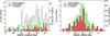 |
Fig. 7 Galactic longitude (left) and latitude size (right) distributions for candidate (green) and known (red) SNRs. The light gray histograms show the distribution of H ii regions from the WISE catalog. The longitude distributions of the candidate and known SNRs are similar, with the most obvious exception being the larger number of candidates near ℓ = 30°. The Galactic latitude distributions in the right panel are not statistically different, nor are they different from that of H ii regions. There is no indication that the SNR sample is significantly incomplete near b = 0° where confusion is the greatest. |
The discrepancy between the number of SNRs and the number of H ii regions may give some clues about the recent star formation rate. While H ii regions primarily trace younger O-stars, SNRs arise from both O and B-stars. Since B-stars are on average older than O-stars, SNRs trace an older stellar population than H ii regions. Young massive star formation regions are thus more likely to have a higher ratio of H ii regions to SNRs. For example, the W49 region near ℓ = 43° is known to have an age of ~ 1.5 Myr (Wu et al. 2016), which is less than the lifetime of the most massive O-stars. The large number of H ii regions here relative to the SNR population is consistent with this interpretation. There are similar discrepancies near ℓ = 49°, associated with W51, and ℓ = 25°. It is worth noting that W51 does host a large, luminous SNR G49.2−0.7, implying that there were multiple generations of star formation in the region. In contrast, there is no single large H ii region complex near l = 25°.
The Galactic latitude distributions in the right panel of Fig. 7 are similar for the known and candidate SNRs. Both distributions are peaked near b = 0°, but the candidates are skewed more toward positive latitudes compared with the G14 regions. K-S tests show that these differences are not significant, and the latitude distributions of the two populations are not statistically different from that of H ii regions from the WISE catalog. Based on the similarity of the H ii region and SNR latitude distributions, there is no indication that the SNR distribution is missing a significant number of sources near b = 0° where confusion is greatest.
Our distribution of morphological types is heavily skewed toward filled-center morphologies compared with the G14 sample. Of the 52 G14 SNRs in the survey zone, over 75% (41 of 52) are classified as having a shell morphology (including uncertain designations of “S?”; see Table 2). About 15% are classified as having composite morphologies (7 of 52) and ~ 10% are classified as having filled-center morphologies (4 of 52). About half of the SNR candidates with morphological classifications (34 of 69) have shell morphologies, whereas about 40% have filled center morphologies (29 of 69) and about 10% have composite morphologies (6 of 69). The comparatively high percentage of filled-shell SNR candidates may be due to our detection method, which is less biased against a particular morphological type.
As shown in Fig. 8, the candidate SNR angular radius distribution skews toward lower values compared with the distribution for known SNRs. This is expected given the higher resolution THOR+VGPS data compared with previous radio surveys. The average and standard deviation of the candidate and known SNR radii are 6.4′ ± 4.7′ and 11.0′ ± 7.8′, respectively. The two radius distributions are however consistent with originating from a single parent distribution, according to a K-S test. Many of the larger known and candidate SNRs are at higher Galactic longitudes (Fig. 3). Although this may be due to selection effects arising from confusion at lower longitudes, it may also be explained by the fact that the mean heliocentric distance is smaller at higher longitudes.
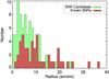 |
Fig. 8 Angular radius distributions for candidate (green) and known (red) SNRs. The candidate SNRs are on average smaller than the known SNRs. |
The angular sizes of the candidate SNRs are on average larger at higher Galactic longitudes. For example the average radius for SNR candidates with ℓ> 35° is 7.6′, whereas it is 5.6′ for candidates with ℓ< 35°. The effect may be real, or may be caused by selection effects. For example, this may indicate that we are unable to identify larger regions in more confused regions at lower Galactic longitudes, or that the angular sizes increase at higher longitudes because the mean heliocentric distance decreases.
The distribution of flux densities derived from THOR+ VGPS data for the new SNR candidates is shifted toward significantly lower values compared with the SNRs in the G14 catalog (Fig. 9). The average and standard deviation of the base-ten logarithm of the G14 sources is 0.82 ± 0.61, while it is −0.23 ± 0.65 for the candidates. A K-S test shows that these differences are statistically significant. The lowest flux G14 sources have flux densities near 1 Jy, although 71% of the candidates have flux densities less than 1 Jy. This result is unsurprising, given that a main advantage of the THOR+VGPS data is that they are more sensitive than previous data. Future surveys, for example with MeerKat, ASKAP, MWA, and LOFAR, will undoubtedly discover additional regions.
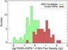 |
Fig. 9 Flux density distribution of new candidate (green) and known (red) SNRs, as measured in the THOR+VGPS data. The distribution of flux densities for the new candidates is shifted toward significantly lower values compared with that of the known sample. |
To investigate whether the detection of the new SNR candidates is due to higher sensitivity or better angular resolution, we examine the flux density versus radius for the G14 and candidate SNRs in Fig. 10. This figure shows that the two populations separate primarily by intensity (see also Fig. 9), but also by radius (see also Fig. 8). Furthermore, all the low-intensity, small radius data points are from THOR SNR candidates.
Surface brightness decreases in Fig. 10 toward the bottom right. There are fractionally more SNR candidates that have lower average surface brightness values compared with the known SNRs. For example, almost half of the candidates fall between the 10-21 and 10-22 W m-2 Hz-1 sr-1 lines whereas only ~ 10% of the known SNRs do. There are nevertheless many G14 SNRs with low surface brightness values similar to those of the THOR candidates. The main advantage of THOR over previous radio continuum data for the present inner-Galaxy study is its improved angular resolution, which allows us to better identify small sources and the thin shells of large sources in complicated fields.
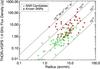 |
Fig. 10 Flux density versus radius for G14 (filled circles) and candidate (plus signs) SNRs. The solid lines show surface brightness limits from 10-19 to 10-22 W m-2 Hz-1 sr-1. The surface brightness therefore decreases from the top left of the plot to the bottom right. The surface brightness distribution of the THOR SNR candidates is similar to that of the known SNRs. |
4.5. Implications for the Galactic SNR population
If confirmed, the 76 new SNR candidates would more than double the known SNR population in the survey zone (52 to 128, not counting the six objects in G14 confused with H ii regions), and will have increased the total Galactic SNR population by 27% (288 to 364, again not counting the six regions). Outside of the Galactic zone surveyed in B06, we identified 67 SNR candidates, two and a half times the 45 known SNRs. The surface brightness limit of the THOR+VGPS data is ~ 10-22 W m-2 Hz-1 sr-1, which given an expected spectral index for SNRs of ~−0.5 is roughly equivalent to that of B06. The THOR+VGPS data are, however, sensitive to a wider range of size scales than the data of B06.
The increase in SNRs suggested by our study is in rough agreement with the prediction of B06. Based on the assumption that future surveys with a similar surface brightness sensitivity would also triple the number of SNRs, B06 predicted there would be ~ 500 SNRs detected in the Galaxy. Even this estimate of ~ 500 is about a factor of two less than expected (see Sect. 1). We agree with B06 that future, more sensitive surveys may resolve the tension, although confusion in the inner Galaxy may limit new detections. Our analysis of Fig. 10 suggests that any future inner-Galaxy survey should prioritize high-angular resolution to reduce confusion.
5. Summary
Using 1.4 GHz continuum data from The H I, OH, and RRL (THOR) VLA survey of the first quadrant of the Galactic plane, combined with continuum data from the VLA Galactic Plane Survey (VGPS), we cataloged 76 new Galactic supernova remnants (SNRs). Our method identifies diffuse radio continuum emission regions lacking mid-infrared counterparts seen for H ii regions and planetary nebulae. All candidates lack MIR emission from known H ii regions, as cataloged in the WISE Catalog of Galactic H ii Regions. The detected candidates follow a similar spatial distribution compared to the previously known sample, albeit with a larger concentration near ℓ = 30°. The low number of known and candidate SNRs near ℓ ≃ 49° (associated with W51), 43° (associated with W49), and 25° relative to the number of H ii regions indicates the relative youth of these star formation regions. The sizes of the new SNR candidates are on average smaller than those of the known regions and the candidate fluxes are on average lower than those of previously known SNRs.
We also detect radio continuum emission from 52 known SNRs from Green (2014), but fail to detect one SNRs in the surveyed region that has a previous radio continuum detection. We note that six known SNRs are confused with H ii regions, and that a further 17 SNR candidates from B06 and H06 are confused with H ii regions. These results show that our method is useful for classifying SNRs mis-identified previously.
If our candidates prove to be true SNRs, they would more than double the Galactic SNR population in the surveyed region. Even with this large number of new candidates, there is still a factor of two disagreement between the number of SNRs detected and the number expected. Similar studies in other parts of the Galaxy using data as sensitive as THOR could further reduce the discrepancy, although confusion in the inner Galaxy is likely to make subsequent detections increasingly difficult. To maximize SNR detections, such future surveys of the inner Galaxy should also have high angular resolution.
Acknowledgments
The National Radio Astronomy Observatory is a facility of the National Science Foundation operated under cooperative agreement by Associated Universities, Inc. H.B. and Y.W. acknowledge support from the European Research Council under the Horizon 2020 Framework Program via the ERC Consolidator Grant CSF-648505. R.S.K. and S.C.O.G. acknowledge support from the European Research Council via the ERC Advanced Grant STARLIGHT (project number 339177). They furthermore thank the DFG for financial help via SFB 881 “The Milky Way System” (subprojects B1, B2, and B8) and SPP 1573 “Physics of the Interstellar Medium”. F.B. acknowledges support from DFG grant BI 1546/1-1.
References
- Anderson, L. D., Bania, T. M., Balser, D. S., & Rood, R. T. 2011, ApJS, 194, 32 [NASA ADS] [CrossRef] [Google Scholar]
- Anderson, L. D., Zavagno, A., Barlow, M. J., García-Lario, P., & Noriega-Crespo, A. 2012, A&A, 537, A1 [NASA ADS] [CrossRef] [EDP Sciences] [Google Scholar]
- Anderson, L. D., Bania, T. M., Balser, D. S., et al. 2014, ApJS, 212, 1 [NASA ADS] [CrossRef] [Google Scholar]
- Anderson, L. D., Deharveng, L., Zavagno, A., et al. 2015, ApJ, 800, 101 [NASA ADS] [CrossRef] [Google Scholar]
- Benjamin, R. A., Churchwell, E., Babler, B. L., et al. 2003, PASP, 115, 953 [NASA ADS] [CrossRef] [Google Scholar]
- Benjamin, R. A., Churchwell, E., Babler, B. L., et al. 2005, ApJ, 630, L149 [NASA ADS] [CrossRef] [Google Scholar]
- Beuther, H., Bihr, S., Rugel, M., et al. 2016, A&A, 595, A32 [NASA ADS] [CrossRef] [EDP Sciences] [Google Scholar]
- Bihr, S., Johnston, K. G., Beuther, H., et al. 2016, A&A, 588, A97 [NASA ADS] [CrossRef] [EDP Sciences] [Google Scholar]
- Brogan, C. L., Gelfand, J. D., Gaensler, B. M., Kassim, N. E., & Lazio, T. J. W. 2006, ApJ, 639, L25 [NASA ADS] [CrossRef] [Google Scholar]
- Carey, S. J., Noriega-Crespo, A., Mizuno, D. R., et al. 2009, PASP, 121, 76 [NASA ADS] [CrossRef] [Google Scholar]
- Churchwell, E., Babler, B. L., Meade, M. R., et al. 2009, PASP, 121, 213 [NASA ADS] [CrossRef] [Google Scholar]
- Cohen, M., & Green, A. J. 2001, MNRAS, 325, 531 [NASA ADS] [CrossRef] [Google Scholar]
- Condon, J. J., Cotton, W. D., Greisen, E. W., et al. 1998, AJ, 115, 1693 [NASA ADS] [CrossRef] [Google Scholar]
- de Avillez, M. A., & Breitschwerdt, D. 2005, A&A, 436, 585 [NASA ADS] [CrossRef] [EDP Sciences] [Google Scholar]
- Douvion, T., Lagage, P. O., Cesarsky, C. J., & Dwek, E. 2001, A&A, 373, 281 [NASA ADS] [CrossRef] [EDP Sciences] [Google Scholar]
- Faucher-Giguère, C.-A., Quataert, E., & Hopkins, P. F. 2013, MNRAS, 433, 1970 [NASA ADS] [CrossRef] [Google Scholar]
- Girichidis, P., Walch, S., Naab, T., et al. 2016, MNRAS, 456, 3432 [NASA ADS] [CrossRef] [Google Scholar]
- Green, A. J., Reeves, S. N., & Murphy, T. 2014, PASA, 31, e042 [NASA ADS] [CrossRef] [Google Scholar]
- Green, D. A. 2004, Bull. Astron. Soc. India, 32, 335 [NASA ADS] [Google Scholar]
- Green, D. A. 2014, Bull. Astron. Soc. India, 42, 47 [NASA ADS] [Google Scholar]
- Green, D. A. 2015, MNRAS, 454, 1517 [NASA ADS] [CrossRef] [Google Scholar]
- Gregory, P. C., Scott, W. K., Douglas, K., & Condon, J. J. 1996, ApJS, 103, 427 [NASA ADS] [CrossRef] [Google Scholar]
- Haslam, C. G. T., & Osborne, J. L. 1987, Nature, 327, 211 [NASA ADS] [CrossRef] [Google Scholar]
- Helfand, D. J., Becker, R. H., White, R. L., Fallon, A., & Tuttle, S. 2006, AJ, 131, 2525 [NASA ADS] [CrossRef] [Google Scholar]
- Joung, M. R., Mac Low, M.-M., & Bryan, G. L. 2009, ApJ, 704, 137 [NASA ADS] [CrossRef] [Google Scholar]
- Lang, C. C., Wang, Q. D., Lu, F., & Clubb, K. I. 2010, ApJ, 709, 1125 [NASA ADS] [CrossRef] [Google Scholar]
- Li, Z., Wheeler, J. C., Bash, F. N., & Jefferys, W. H. 1991, ApJ, 378, 93 [NASA ADS] [CrossRef] [Google Scholar]
- Lockman, F. J. 1989, ApJS, 71, 469 [NASA ADS] [CrossRef] [Google Scholar]
- Lockman, F. J., Pisano, D. J., & Howard, G. J. 1996, ApJ, 472, 173 [NASA ADS] [CrossRef] [Google Scholar]
- Luisi, M., Anderson, L. D., Balser, D. S., Bania, T. M., & Wenger, T. V. 2016, ApJ, 824, 125 [NASA ADS] [CrossRef] [Google Scholar]
- Ostriker, E. C., & Shetty, R. 2011, ApJ, 731, 41 [NASA ADS] [CrossRef] [Google Scholar]
- Ostriker, E. C., McKee, C. F., & Leroy, A. K. 2010, ApJ, 721, 975 [NASA ADS] [CrossRef] [Google Scholar]
- Padoan, P., Pan, L., Haugbølle, T., & Nordlund, Å. 2016, ApJ, 822, 11 [NASA ADS] [CrossRef] [Google Scholar]
- Pinheiro Gonçalves, D., Noriega-Crespo, A., Paladini, R., Martin, P. G., & Carey, S. J. 2011, AJ, 142, 47 [NASA ADS] [CrossRef] [Google Scholar]
- Reach, W. T., Rho, J., Tappe, A., et al. 2006, AJ, 131, 1479 [NASA ADS] [CrossRef] [Google Scholar]
- Reich, P., & Reich, W. 1986, A&AS, 63, 205 [NASA ADS] [Google Scholar]
- Reich, W., Reich, P., & Fuerst, E. 1990, A&AS, 83, 539 [NASA ADS] [Google Scholar]
- Rho, J., Kozasa, T., Reach, W. T., et al. 2008, ApJ, 673, 271 [NASA ADS] [CrossRef] [Google Scholar]
- Sabin, L., Parker, Q. A., Contreras, M. E., et al. 2013, MNRAS, 431, 279 [NASA ADS] [CrossRef] [Google Scholar]
- Stil, J. M., Taylor, A. R., Dickey, J. M., et al. 2006, AJ, 132, 1158 [NASA ADS] [CrossRef] [Google Scholar]
- Sun, X. H., Reich, P., Reich, W., et al. 2011, A&A, 536, A83 [NASA ADS] [CrossRef] [EDP Sciences] [Google Scholar]
- Tammann, G. A., Loeffler, W., & Schroeder, A. 1994, ApJS, 92, 487 [NASA ADS] [CrossRef] [Google Scholar]
- Williams, B. J., Borkowski, K. J., Reynolds, S. P., et al. 2006, ApJ, 652, L33 [NASA ADS] [CrossRef] [Google Scholar]
- Wright, E. L., Eisenhardt, P. R. M., Mainzer, A. K., et al. 2010, AJ, 140, 1868 [NASA ADS] [CrossRef] [Google Scholar]
- Wu, S.-W., Bik, A., Bestenlehner, J. M., et al. 2016, A&A, 589, A16 [NASA ADS] [CrossRef] [EDP Sciences] [Google Scholar]
Appendix A: SNR images
Here we provide THOR+VGPS 1.4 GHz images for the individual candidate SNRs.
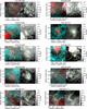 |
Fig. A.1 Images for all identified SNR candidates. The left panels show two-color GLIMPSE 8.0 μm (cyan) and THOR+VGPS 21 cm (red), as in Fig. 1. The right panels show THOR+VGPS data alone. Circles in both panels are the same as in Fig. 1, with candidate SNRs are enclosed by green circles, known SNRs by red circles, and known or candidate H ii regions by white circles. |
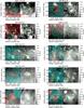 |
Fig. A.1 continued. |
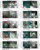 |
Fig. A.1 continued. |
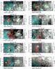 |
Fig. A.1 continued. |
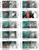 |
Fig. A.1 continued. |
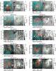 |
Fig. A.1 continued. |
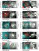 |
Fig. A.1 continued. |
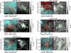 |
Fig. A.1 continued. |
All Tables
All Figures
|
Fig. 1 (Top) Two-color images with GLIMPSE 8.0 μm data in cyan and THOR+VGPS 21 cm continuum data in red. H ii regions have 8.0 μm emission surrounding the 21 cm emission. Although not shown, MIPSGAL 24 μm emission has a similar morphology as the radio continuum for H ii regions, and is essentially absent for SNRs. The candidate SNRs are enclosed by green circles, known SNRs by red circles, and known or candidate H ii regions by white circles. Dotted boxes enclose the areas displayed as insets below. These insets show a known H ii region that has bright 8.0 μm emission (left; G028.022−00.043), a known SNR (middle; G27.4+0.0), and an example SNR candidate (right; G26.75+0.73). The H ii region has strong 8.0 μm emission surrounding the radio continuum, but the known and candidate SNRs are devoid of 8.0 μm emission. |
| In the text | |
|
Fig. 2 Example images for select SNR candidates, showing the range of surface brightnesses and morphologies. The left panels show two-color GLIMPSE 8.0 μm (cyan) and THOR+VGPS 21 cm (red), as in Fig. 1. The right panels show THOR+VGPS data alone. Circles in both panels are the same as in Fig. 1, with candidate SNRs are enclosed by green circles, known SNRs by red circles, and known or candidate H ii regions by white circles. |
| In the text | |
|
Fig. 3 Galactic distribution of the new candidate (green) and known (red) SNRs. The circles approximate the SNR sizes, but due to the aspect ratio of the plot, the sizes are only valid along the Galactic longitude axis. The background is a two-dimensional histogram of the H ii region density, with higher densities indicated by darker colors. |
| In the text | |
|
Fig. 4 THOR+VGPS 1.4 GHz flux densities compared with G14 1 GHz flux densities. Filled circles denote SNRs that have more secure values in the G14 catalog, whereas open circles are more uncertain (values that have a question mark in the G14 catalog). The dotted line shows a 1:1 relationship. |
| In the text | |
|
Fig. 5 G14 SNRs confused with H ii regions. Shown for each region are two-color images with GLIMPSE 8.0 μm (for G20.4+0.1, G21.5−0.1, G23.6+0.3, and G54.1+0.3) or WISE 12 μm data (for G59.8+1.2 and G65.8−0.5) in cyan and THOR+VGPS 21 cm continuum data in red. The central positions are taken from the G14 catalog, and the image dimensions are three times the G14 SNR diameters. As in Fig. 1, the candidate SNRs are enclosed by green circles and known or candidate H ii regions by white circles. Red dotted circles show the expected position and size of the G14 SNRs that are confused with H ii regions. |
| In the text | |
|
Fig. 6 Mis-identified SNR candidates from H06 and B06. The format for these images is the same as that of Fig. 1, with GLIMPSE 8.0 μm data in cyan and THOR+VGPS 21 cm continuum data in red. As in Fig. 1, the candidate SNRs are enclosed by green circles, known SNRs by red circles, and known or candidate H ii regions by white circles. Red dotted circles show the expected position and size of the SNR candidates. All except for G19.1+0.9, which appears to be a radio continuum filament, and G29.0778+0.4542, which is a planetary nebula, are confused with H ii regions. |
| In the text | |
|
Fig. 7 Galactic longitude (left) and latitude size (right) distributions for candidate (green) and known (red) SNRs. The light gray histograms show the distribution of H ii regions from the WISE catalog. The longitude distributions of the candidate and known SNRs are similar, with the most obvious exception being the larger number of candidates near ℓ = 30°. The Galactic latitude distributions in the right panel are not statistically different, nor are they different from that of H ii regions. There is no indication that the SNR sample is significantly incomplete near b = 0° where confusion is the greatest. |
| In the text | |
|
Fig. 8 Angular radius distributions for candidate (green) and known (red) SNRs. The candidate SNRs are on average smaller than the known SNRs. |
| In the text | |
|
Fig. 9 Flux density distribution of new candidate (green) and known (red) SNRs, as measured in the THOR+VGPS data. The distribution of flux densities for the new candidates is shifted toward significantly lower values compared with that of the known sample. |
| In the text | |
|
Fig. 10 Flux density versus radius for G14 (filled circles) and candidate (plus signs) SNRs. The solid lines show surface brightness limits from 10-19 to 10-22 W m-2 Hz-1 sr-1. The surface brightness therefore decreases from the top left of the plot to the bottom right. The surface brightness distribution of the THOR SNR candidates is similar to that of the known SNRs. |
| In the text | |
|
Fig. A.1 Images for all identified SNR candidates. The left panels show two-color GLIMPSE 8.0 μm (cyan) and THOR+VGPS 21 cm (red), as in Fig. 1. The right panels show THOR+VGPS data alone. Circles in both panels are the same as in Fig. 1, with candidate SNRs are enclosed by green circles, known SNRs by red circles, and known or candidate H ii regions by white circles. |
| In the text | |
|
Fig. A.1 continued. |
| In the text | |
|
Fig. A.1 continued. |
| In the text | |
|
Fig. A.1 continued. |
| In the text | |
|
Fig. A.1 continued. |
| In the text | |
|
Fig. A.1 continued. |
| In the text | |
|
Fig. A.1 continued. |
| In the text | |
|
Fig. A.1 continued. |
| In the text | |
Current usage metrics show cumulative count of Article Views (full-text article views including HTML views, PDF and ePub downloads, according to the available data) and Abstracts Views on Vision4Press platform.
Data correspond to usage on the plateform after 2015. The current usage metrics is available 48-96 hours after online publication and is updated daily on week days.
Initial download of the metrics may take a while.