| Issue |
A&A
Volume 693, January 2025
|
|
|---|---|---|
| Article Number | A247 | |
| Number of page(s) | 11 | |
| Section | Interstellar and circumstellar matter | |
| DOI | https://doi.org/10.1051/0004-6361/202451038 | |
| Published online | 22 January 2025 | |
Supernova remnant candidates discovered by the SARAO MeerKAT Galactic Plane Survey
1
Department of Physics and Astronomy, West Virginia University,
Morgantown,
WV
26506,
USA
2
Adjunct Astronomer at the Green Bank Observatory,
PO Box 2,
Green Bank,
WV
24944,
USA
3
Center for Gravitational Waves and Cosmology, West Virginia University,
Chestnut Ridge Research Building,
Morgantown,
WV
26505,
USA
4
South African Radio Astronomy Observatory,
2 Fir Street,
Observatory
7925,
South Africa
5
SARAO/Hartebeesthoek Radio Astronomy Observatory,
PO Box 443,
Krugersdorp
1740,
South Africa
6
Department of Physics and Astronomy, York University,
Toronto
M3J 1P3,
Ontario,
Canada
7
INAF – Osservatorio Astrofisico di Catania,
Via S. Sofia 78,
95123
Catania,
Italy
8
Department of Mathematical Sciences, University of South Africa,
Cnr Christian de Wet Rd and Pioneer Avenue, Florida Park,
1709,
Roodepoort,
South Africa
9
Centre for Space Research, Physics Department, North-West University,
Potchefstroom
2520,
South Africa
10
Department of Physics and Astronomy, Faculty of Physical Sciences, University of Nigeria,
Carver Building, 1 University Road,
Nsukka
410001,
Nigeria
11
National Radio Astronomy Observatory,
520 Edgemont Road,
Charlottesville,
VA
22903,
USA
12
School of Physics and Astronomy, University of Leeds,
Leeds
LS2 9JT,
UK
13
Department of Physics, Aberystwyth University,
Ceredigion,
Cymru SY23 3BZ,
UK
★ Corresponding author; This email address is being protected from spambots. You need JavaScript enabled to view it.
Received:
8
June
2024
Accepted:
20
September
2024
Abstract
Context. Sensitive radio continuum data could bring the number of known supernova remnants (SNRs) in the Galaxy more in line with what is expected. Due to confusion in the Galactic plane, however, faint SNRs can be challenging to distinguish from brighter H II regions and filamentary radio emission.
Aims. We exploited new 1.3 GHz SARAO MeerKAT Galactic Plane Survey (SMGPS) radio continuum data, which cover 251° ≤ ℓ ≤ 358° and 2° ≤ ℓ ≤ 61° at | b | ≤ 1.5°, to search for SNR candidates in the Milky Way disk.
Methods. We also used mid-infrared data from the Spitzer GLIMPSE, Spitzer MIPSGAL, and WISE surveys to help identify SNR candidates. These candidates are sources of extended radio continuum emission that lack mid-infrared counterparts, are not known as H II regions in the WISE Catalog of Galactic H II Regions, and have not been previously identified as SNRs.
Results. We locate 237 new Galactic SNR candidates in the SMGPS data. We also identify and confirm the expected radio morphology for 201 objects classified in the literature as SNRs and 130 previously identified SNR candidates. The known and candidate SNRs have similar spatial distributions and angular sizes.
Conclusions. The SMGPS data allowed us to identify a large population of SNR candidates that can be confirmed as true SNRs using radio polarization measurements or by deriving radio spectral indices. If the 237 candidates are confirmed as true SNRs, it would approximately double the number of known Galactic SNRs in the survey area, alleviating much of the discrepancy between the known and expected populations.
Key words: H II regions / ISM: supernova remnants / radio continuum: ISM
© The Authors 2025
 Open Access article, published by EDP Sciences, under the terms of the Creative Commons Attribution License (https://creativecommons.org/licenses/by/4.0), which permits unrestricted use, distribution, and reproduction in any medium, provided the original work is properly cited.
This article is published in open access under the Subscribe to Open model. This email address is being protected from spambots. You need JavaScript enabled to view it. to support open access publication.
1 Introduction
The number of confirmed Galactic supernova remnants (SNRs) is only a few hundred according to the two most authoritative catalogs: that of Green (2022, hereafter G22)1, which contains 303 SNRs2, and SNRCat (Ferrand & Safi-Harb 2012), which lists 383 objects in its online catalog3. Based on OB star counts, pulsar birth rates, Fe abundances, and the supernova rate in other Local Group galaxies, there should be ≳1000 Galactic SNRs (Li et al. 1991; Tammann et al. 1994). Ranasinghe & Leahy (2022) suggest that there may actually be a few thousand Galactic SNRs based on the population detected to date and on SNR search selection effects. The discrepancy between the identified population of Galactic SNRs and the expected number is likely due to a lack of sensitive radio continuum data and confusion in the Galactic plane (e.g., Brogan et al. 2006; Ranasinghe & Leahy 2022).
The Galactic supernova rate is key to understanding the properties and dynamics of the Milky Way. The number of SNRs in the Galaxy is related to recent massive star formation activity (see Tammann et al. 1994). Supernovae inject energy into the interstellar medium (ISM), driving molecular cloud turbulence and galactic fountains out of the disk (de Avillez & Breitschwerdt 2005; Joung et al. 2009; Padoan et al. 2016; Girichidis et al. 2016); they therefore affect the disk scale height and star formation properties of a galaxy (Ostriker et al. 2010; Ostriker & Shetty 2011; Faucher-Giguère et al. 2013).
Supernova remnants can be most efficiently identified using radio data. According to our assessment of the G22 catalog, ~90% of known SNRs are detected and well defined in the radio regime, ~40% are detected in X-rays, and ~30% in the optical. More sensitive radio observations may increase the number detected further. The most common radio morphology in the G22 catalog, accounting for ~80% of the SNRs, is that of a limb-brightened shell or a partial shell, where the diameter of the shell is set by the expanding shock wave produced by the explosion. SNRs can also be classified as “filled-center” or “plerions” if they have centrally concentrated radio emission, which is is generally caused by a pulsar wind nebula (PWN; e.g., the Crab nebula; Weiler & Sramek 1988; Bietenholz et al. 2015), or “composite” if the SNR appears to have both a shell and an internal component (either a nonthermally emitting pulsar-driven nebula or a thermally emitting X-ray source; see Dubner & Giacani 2015 for a review of radio SNR morphologies).
Separating nonthermally emitting SNRs from the much more common thermally emitting H II regions in the Galactic plane is challenging. There are ≳ 7000 identified Galactic H II regions (Armentrout et al. 2021). If there are data at multiple radio frequencies, one can compute the spectral index, α, as S ∝ vα, with S being the flux density and ν the frequency4. Most SNRs have spectral indices in the range α = −0.8 to α = 0.0, whereas H II regions should have α ~ −0.1 if optically thin and α > −0.1 if optically thick. Although a spectral index value near 0 does not allow us to discriminate between the two classifications, values α ≲ −0.2 indicate nonthermal emission and, therefore, an SNR rather than an H II region. The computation of the spectral index, however, is difficult because all radio continuum datasets must have sensitivity to the same spatial scales. Also, filled-center SNRs may have spectral indices near −0.1 (e.g., Bietenholz & Bartel 2008 find α = 0.08 for G21.5−0.5). An additional indication of nonthermal emission is the presence of polarized radio continuum emission, although due to the fact that the polarized emission fraction is often quite low, this criterion is also difficult to apply (Dokara et al. 2018). In a SNR, the intrinsic polarization angle usually follows the bright ridges of emission (e.g., Cotton et al. 2024), but the presence of polarized emission in the same direction as a SNR does not necessarily mean that it is a SNR.
A simpler and perhaps more reliable criterion for separating H II regions from SNRs is the mid-infrared (MIR) to radio continuum flux ratio. Although MIR emission can be detected from SNRs in some cases (Reach et al. 2006; Pinheiro Gonçalves et al. 2011), many researchers have shown that SNRs have less MIR emission than H II regions (e.g., Cohen & Green 2001; Pinheiro Gonçalves et al. 2011). The MIR to radio flux ratio for SNRs is about 100 times lower than that of optically thin H II regions.
In the last decade, studies of radio continuum and infrared data have identified a large number of Galactic SNR candidates. Those that have been confirmed as SNRs are in the SNR catalogs discussed above, but the majority are awaiting confirmation. Green et al. (2014) used the anticorrelation between radio and 8 µm emission to locate 23 new SNR candidates from 843 MHz Molonglo Galactic Plane Survey (MGPS) data.
Anderson et al. (2017) used 1.4 GHz continuum data from The H I, OH, Recombination line survey of the Milky Way (THOR; Beuther et al. 2016), combined with the 1.4 GHz radio continuum data from the Very Large Array Galactic Plane Survey (VGPS; Stil et al. 2006), to identify 76 new SNR candidates. Dokara et al. (2018) confirmed 2 of these 76 candidates as true SNRs using spectral index measurements. Hurley-Walker et al. (2019) found 27 new SNRs using data from the GaLactic and Extragalactic All-sky Murchison Widefield Array (GLEAM) survey and confirmed 26 of them using spectral index measurements; these 26 are listed as known SNRs in G22. Dokara et al. (2021) used data from the 4–8 GHz GLObal view of STAR formation in the Milky Way (GLOSTAR; Brunthaler et al. 2021) survey to identify 157 SNR candidates, 9 of which have nonthermal emission based on polarization measurements. And, finally, Ball et al. (2023) identified 13 new Galactic SNR candidates in 933 MHz Australian Square Kilometre Array Pathfinder (ASKAP) data. These studies followed those of Helfand et al. (2006), who discovered 49 new SNR candidates in the MultiArray Galactic Plane Imaging Survey (MAGPIS) 20 cm data, and Brogan et al. (2006), who discovered 35 SNR candidates in their VLA data. Even if all the recently identified SNR candidates are confirmed as true SNRs, there remains a discrepancy between the number of detected Galactic SNRs and the expected number.
Here, we used new 1.3 GHz South African Radio Astronomy Observatory (SARAO) MeerKAT Galactic Plane Survey (SMGPS) data to identify SNR candidates in the inner Galaxy. This work complements that of Bordiu et al. (2024), who used SMGPS data to create an extended source catalog, and Loru et al. (2024), who provide an in-depth study of 28 Galactic SNRs in SMGPS data for which flux and spectral indices can be derived.
2 Data
2.1 SARAO MeerKAT Galactic Plane Survey (SMGPS)
The ideal radio continuum dataset for SNR searches is sensitive to large, extended structures but also boasts high angular resolution. Extended source sensitivity is necessary for the detection of low surface brightness SNRs and high angular resolution allows one to disentangle the complicated emission of the Galactic plane.
The 1.3 GHz SMGPS (Goedhart et al. 2024)5 covers 251° ≤ ℓ ≤ 358° and 2° ≤ ℓ ≤ 61° at | b | ≤ 1.5°. The boundaries at high and low Galactic latitudes are slightly irregular because the survey follows the Galactic warp. A full description of the radio observations and the data reduction procedures is provided in Goedhart et al. (2024). Observations used the 64 antenna MeerKAT array in the Northern Cape Province of South Africa, which is described in Jonas & MeerKAT Team (2016), Camilo et al. (2018), and Mauch et al. (2020). We used here the “zeroth moment” data, which have a central frequency of 1293 MHz with a total used bandwidth of 672 MHz (these values both decrease at high and low Galactic latitudes; see Goedhart et al. 2024). The angular resolution is ~8″ and the data are sensitive to emission up to angular scales of ~30′. The background rms noise in areas far from the Galactic Plane and bright point sources is ~30 µJybeam−1. The low surface brightness noise threshold together with the sensitivity to both large and small-scale structures makes the SMGPS survey the ideal dataset to identify new SNRs.
2.2 MIR data
Over the zone 65° > ℓ > −100°, | b | < 1.0° we used Spitzer 8.0 and 3.6 µm data from the Galactic Legacy Infrared MidPlane Survey Extraordinaire (GLIMPSE; Benjamin et al. 2003; Churchwell et al. 2009) and 24 µm data from the MIPSGAL survey (Carey et al. 2009). Outside this zone we used data from the all-sky Widefield Infrared Survey Explorer (WISE; Wright et al. 2010) at 12 and 22 µm. Since the GLIMPSE and MIPSGAL surveys have a better angular resolution and sensitivity than that of WISE, we used Spitzer data when possible.
H II regions have strong emission at these wavelengths. The ~10 µm emission is largely from polycyclic aromatic hydrocarbons (PAHs), which fluoresce in the presence of soft ultra-violet (~5 eV) radiation (Voit 1992) and the ~20 µm emission is mainly from small dust grains co-spatial with the H II region plasma.
For most SNRs, MIR emission at these wavelengths is largely absent, or at least is at a low intensity compared to that of H II regions (e.g., Cohen & Green 2001; Pinheiro Gonçalves et al. 2011). Some young SNRs do have strong MIR emission, however, especially at ~20 µm. The origin of this emission is dust, atomic or molecular ine emission, or synchrotron emission, with the relative importance of each depending on the SNR in question (see Gonçalves et al. 2011, for a concise summary).
2.3 The WISE Catalog of Galactic H II Regions
The WISE Catalog of Galactic H II Regions (Anderson et al. 2014, hereafter the WISE Catalog) is the largest catalog of Galactic H II regions. All catalog entries have WISE (Wright et al. 2010) ~20 µm emission surrounded by ~10 µm emission (Anderson et al. 2011). The WISE catalog contains ~8000 objects with the MIR morphology of H II regions. The ~20 µm emission from H II regions is caused by small stochastically heated dust grains that are mixed with the H II region plasma, while the ~10 µm intensity is dominated by emission from PAHs. All known Galactic H II regions have this characteristic morphology. Here, we used Version 3.0 of the catalog6.
2.4 SNR catalogs
The G22 catalog currently contains 303 regions compiled from the literature. Green (2004) suggest that a previous (but similar) version of the catalog was largely complete to a radio surface density limit of 10−20 W m−2 Hz−1 sr−1 (1 MJysr−1). At the 8″ resolution of the SMGPS data, this corresponds to 1.7 mJy beam−1, or ~60 times greater than the SMGPS 1σ point source sensitivity. In addition to the surface brightness limit, the catalog appears to be lacking the small angular size SNRs that are expected (Green 2015).
SNRCat (Ferrand & Safi-Harb 2012) contains 383 entries in the most recent online version and focuses largely on their high energy emission. All G22 sources are also included in SNRCat. Even though there are more entries than in G22, many of these are not the same as the SNRs listed in G22; SNRCat includes PWNe, bow-shock nebulae, high-energy (X-ray and gamma-ray) discovered SNRs, and magnetar-hosting SNRs.
As there are significant differences in their compositions, we treated G22 and SNRCat separately. Although both catalogs cover the entire sky, since they are not derived from homogeneous datasets, the catalog sensitivities vary with Galactic location. Both catalogs contain at a minimum spatial coordinates and angular sizes for all entries. When the extent of the SNR is listed with an ellipse, we instead used a circle that has an angular radius that is an average between that of the semimajor and semiminor axes.
2.5 SNR candidate catalogs
There are numerous extant catalogs of SNR candidates. We primarily used the compilation of previously known and newly discovered SNR candidates in Dokara et al. (2021), which includes results from Brogan et al. (2006), Helfand et al. (2006), Anderson et al. (2017), and Hurley-Walker et al. (2019). We supplemented this list using the results from numerous other studies compiled in the G22 documentation and added the recent study of Ball et al. (2023). Over the SMGPS range, there are 190 SNR candidates; 74 of these were compiled by Dokara et al. (2021), and 78 were identified for the first time by Dokara et al. (2021).
As with the known SNRs, in cases where the extent of the SNR candidate is defined with an ellipse, we instead used a circle that has a radius in between that of the semimajor and semiminor axes.
3 Method
The present study has two main goals: (1) to assess the radio emission from known and candidate SNRs in the SMGPS data and (2) to identify new SNR candidates.
For the first goal, we inspect SMGPS and MIR data at the positions of all known and candidate SNRs from the catalogs in Sects. 2.4 and 2.5. We take the coordinates of a given object from the most recent published study, which is not necessarily the same as that listed in the catalogs. During this visual inspection, we primarily seek to ascertain if the identified SNR or SNR candidate is detected in the SMGPS. If it is, we determine if it is confused with an H II region.
For the second goal, our identification methodology was similar to that used by numerous recent authors (e.g., Anderson et al. 2017; Dokara et al. 2021; Ball et al. 2023): we identified discrete regions of radio continuum emission that (1) have a radio morphology consistent with known SNRs (i.e., roughly circular), (2) are not identified as being H II regions in the WISE Catalog, known SNRs, or SNR candidates, and (3) lack Spitzer or WISE MIR emission characteristic of thermal sources. Criteria 2 and 3 are somewhat redundant as nearly all discrete sources of coincident MIR and radio continuum emission in the Galactic plane are H II regions and are included in the WISE catalog. As mentioned previously, some SNRs do have MIR emission, but the quality of this emission differs between SNRs and H II regions. Aside from the radio-to-MIR flux ratio being higher for SNRs than for H II regions (e.g., Cohen & Green 2001; Pinheiro Gonçalves et al. 2011), the ~24 µm emission for SNRs more closely follows the radio than for H II regions, and there is no related ~10µm emission.
We illustrate the by-eye identification process in Fig. 1. We first identify the SMGPS emission associated with all known SNRs and SNR candidates (red and green circles, respectively). We then identify all discrete, extended radio continuum sources that are not associated with these SNRs or SNR candidates, and also are not associated with H II regions in the WISE Catalog. We classify such sources as new SNR candidates (light green) or unusual objects (pink). We inspect each SMGPS field on three separate occasions to ensure that we identify as many SNR candidates as possible.
We do not have a preferred morphology for the identified SNR candidates aside from requiring that the emission is relatively circularly symmetric. We then searched the MIR data for emission of a complementary morphology to that of the SMGPS data, which allowed us to remove any remaining H II regions not included in the WISE Catalog. We classified the remaining radio continuum sources are SNR candidates.
We approximated the center and angular extent of each identified object by defining a circle that encloses its SMGPS emission. Our method therefore defines new positions for all known and candidate SNRs in the SMGPS zone. For partial shells, the defined circle follows the curvature of the shell. Also, if the source is partially off the SMGPS zone, we defined the circle following the emission that is detected; such centroids and radii can therefore be quite uncertain.
For each newly identified SNR candidate, we queried the SIMBAD database7, with a search radius of 5′. This process allows us to remove previously identified objects from the sample.
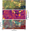 |
Fig. 1 Example field centered at (ℓ, b) = (324.0°, −0.2°). Top: Spitzer three-color data, with MIPSGAL 24 µm data in red, GLIMPSE 8.0 µm data in green, and GLIMPSE 3.6 µm data in blue. Middle: 1.3 GHz SMGPS data. Bottom: 1.3 GHz SMGPS data in red, MIPSGAL 24 µm data in green, and GLIMPSE 8.0 µm data in blue. White circles show HII regions from the WISE Catalog (Sect. 2.3), blue-green circles previously known SNRs (Sect. 4.1), green circles previously known SNR candidates (Sect. 4.2), light green circles SNR candidates newly identified here (Sect. 4.3), and yellow circles “unusual” sources (Sect. 4.4). Although there are no examples in this field, in subsequent figures we show misidentified or undetected SNRs and SNR candidates with dashed circles. |
Sources studied.
4 Results
We summarize the results of our investigation of previously known SNRs, previously identified SNR candidates, and newly discovered sources in Table 1. This table lists for each category the number of objects, and the number confirmed as SNRs or SNR candidates (if previously known). We give more details on these samples in the following subsections.
4.1 Previously identified SNRs
We detect SMGPS emission from all 187 G22 SNRs whose centroids fall within the SMGPS area. Of these, we confirm 184, listed in Table A.1, and show examples in Fig. 2. In this table we revise the coordinates and sizes of the SNRs to enclose the SMGPS emission, but use the G22 source names.
Although some known SNRs in the sample do have MIR emission, the quality of this emission is very different from that of H II regions. For example, for SNR G11.2−0.3 shown in Fig. 2, there is bright 24 µm emission. Compared to H II regions, however, this source is lacking the ~10 µm emission that delineates a photodissociation region. Therefore, one can visually distinguish between SNRs and H II regions, even for those SNRs that are bright at 24 µm.
We separated one G22 source into two SNRs. The G22 source G337−0.1 is a small, ~1′ diameter object. The larger shell, which was also called G337−0.1 in previous versions of the G22 catalog, is also detected in SMGPS data; we include the larger shell as a separate catalog entry using the name G337-0.1∗. We show these two regions in Fig. 3.
We think that two G22 sources are unlikely to be true SNRs. Although the source G298.5−0.3 is unambiguously detected in SMGPS data, it consists of two linear filaments and has a radio morphology inconsistent with the morphology of known SNRs. It fits the criteria for “unusual” sources discussed later and is included there. This source looks like a convincing SNR in low- resolution radio continuum emission from Whiteoak & Green (1996), but the SMGPS data reveals its true morphology. The source G011.8−00.2 overlaps with the WISE Catalog H II region G011.887−00.253. We show these two sources in Fig. 4.
We detect SMGPS emission from 30 SNRCat objects that are not in the G22 catalog, out of 51 examined. We list the detected SNRCat objects in Table A.2. In this table we revise the coordinates and sizes of the sources to enclose the SMGPS emission, but use the catalog source names.
Of the detected sources, six are compact (~30″ or less) PWNe (G267.0−1.0, G284.0−1.8, G336.4+0.2, G350.2−0.8, G18.0−0.7, and G36.0+0.1). Two are long, linear PWNe (G319.9−0.7 and G337.5−0.1). Five are listed in SNRCat as being PWNe or candidates, but have extended radio continuum emission (G313.3+0.1, G313.6+0.3, G333.9+00.0, G348.9−0.4, and G29.4+0.1). The remaining 17 sources have radio morphologies similar to the SNRs in G22. Of these 17, 15 are listed in Green et al. (2014) as being SNR candidates.
We suggest that nine of the examined SNRCat sources are not true SNRs. Of these, four overlap with WISE Catalog H II regions: G8.3−0.0 overlaps with G008.306−00.084, G10.5−0.0 overlaps with G010.585−00.051, G11.0−1.0 overlaps with G011.182−01.063, and G14.3+0.1 overlaps with G014.303+00.140. The radio emission from one, G354.4+0.0, consists of a broad radio filament and based on their MIR emission four appear to be thermal but are not confused with individual H II regions: G284.2−0.4, G304.1−0.2, G21.9−0.1, and G026.6−0.1.
Additionally, 12 SNRCat sources have no identifiable SMGPS emission: G285.1−00.5, G287.4+00.6, G323.9+00.0, G331.5−00.6, G332.5−00.3, G344.7+00.1, G350.2−00.8, G358.1+00.1, G358.3+00.2, G018.5−00.4, G032.73+0.15, G032.6+00.5, and G044.5−00.2. All except for G331.5−00.6 are listed as being PWNe or candidates, so their lack of SMGPS emission is unsurprising.
4.2 Previously identified SNR candidates
We examined the SMGPS images for radio continuum emission from the 170 previously known SNR candidates in the SMGPS zone. We find unambiguous SMGPS emission consistent with that of known SNRs from 130 SNR candidates. We list these detected SNR candidates in Table A.3. In this table, as with the known SNRs, we revise the coordinates and sizes of the SNR candidates to enclose the SMGPS emission, but use the published source names. These names are based on the published coordinates and have different numbers of significant digits between different authors.
We suggest that 13 previously identified SNR candidates are misidentified. Although detected in SMGPS data, a different classification for these sources is warranted. Two are part of known SNRs (G6.4500−0.5583 is part of SNR G6.5−0.4 and G8.8583−0.2583 is part of G8.7−0.1). Three are confused with other SNR candidates (G005.989+0.019 with G006.199+0.157, G28.92+0.26 with G028.929+0.254, and G039.203+0.811 with G039.038+0.748). Five are confused with H II regions (G331.8−0.0 with G331.834−00.00, G002.228+0.058 with G2.227+0.058, G022.951−0.311 with G22.951−0.311, G028.524+0.268 with G028.647+00.198, and G037.506+0.777 with G037.506+0.777). Sources G324.4−0.2 and G327.1+0.9 (Ball et al. 2023) are MIPSGAL bubbles, which are likely caused by an evolved star. Finally, G339.6−0.6 appears to be a radio galaxy.
Radiation will create ionized gas when impingent on a molecular cloud. Like in an H II region, this ionized gas will emit radio continuum emission and the associated heated dust grains will emit in the MIR. A low-density pathway through the ISM would allow photons from a high-mass star formation region to irradiate clouds far afield, making this scenario possible whenever the ionizing flux in a region of the ISM is high. The observational signature of this scenario is MIR emission spatially coincident with radio continuum emission, similar to that of an H II region, but the morphology will not have the generally circular symmetry of an H II region. For six previously identified SNR candidates, we suggest that the emission is actually thermal, caused by irradiation from nearby star formation regions (G26.13+0.13, G028.877+0.241, G28.88+0.41, G34.93−0.24, G39.56−0.32, and G043.070+0.558).
Fifteen previously identified SNR candidates appear to consist of nonthermal radio continuum emission (with no MIR), but the radio emission from each one does not form a cohesive structure (G005.106+0.332, G013.549+0.352, G013.626+0.299, G013.658−0.241, G016.126+0.690, G18.53−0.86, G19.13+0.90, G021.492−0.010, G022.177+0.314, G024.193+0.284, G27.39+0.24, G28.21+0.02, G030.362+0.623, G34.93−0.24, and G037.337+0.422). Most of these consist of a single broad radio filament. We suggest that these sources are poor SNR candidates that deserve future study.
While some previously known SNR candidates are detected in the SMGPS, we decomposed their emission into a number of new SNR candidates or find a dramatically different centroid. We decomposed the SNR candidate G328.6+0.0 (Ball et al. 2023) into two regions. We decomposed SNR candidate G323.6−1.1 (Ball et al. 2023) into two new SNR candidates and the known SNR G323.7−1.0. Finally, we revised the position of G325.8+0.3 substantially. These SNR candidates are not included in Table A.3.
Ten SNR candidates are not detected in SMGPS data: G350.7+0.6, G353.0+0.8, G358.3−0.7, G18.9-1.2, G21.8+0.2, G24.0−0.3, G030.508+0.574, G32.73+0.15, G035.129−0.343, and G35.3−0.0. We can make no judgement on the veracity of these classifications. Most (six of the ten) sources have angular sizes > 30′ , which makes their detection difficult in SMGPS data. Two (G32.73+0.15 and G35.3−0.0) are in regions of the SMGPS with high noise.
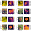 |
Fig. 2 Objects from the G22 catalog. MIR data (Spitzer or WISE) are shown in the left panels and SMGPS 1.3 GHz data in the right. The symbols have the same meaning as in Fig. 1, with the G22 SNRs represented by blue-green circles at the centers of all panels. Cyan scale bars at the lower left of each panel are 5′ long. |
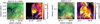 |
Fig. 3 Objects from the G22 catalog split into two entries, G337.0−0.1* and G337.0−0.1. MIR data are shown in the left panels and SMGPS 1.3 GHz data in the right. The symbols have the same meaning as in Fig. 1, with the G22 SNRs represented by blue-green circles at the centers of all panels. Yellow scale bars at the lower left of each panel are 5′ long. |
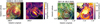 |
Fig. 4 Objects from the G22 catalog that are unlikely to be true SNRs. MIR data are in the left panels (Spitzer or WISE) and SMGPS 1.3 GHz data in the right. The symbols have the same meaning as in Fig. 1, with the G22 SNRs indicated by dashed blue-green circles at the centers of all panels. Yellow scale bars at the lower left of each panel are 5′ long. |
4.3 Newly identified SNR candidates
By visually inspecting SMGPS and MIR data, we identified 237 new SNR candidates8. All 237 SNR candidates have SMGPS 1.3 GHz continuum emission and a deficiency of MIR emission.
For each candidate, we assigned a reliability criterion that indicates our confidence that the object is a true SNR ranging from I (high reliability) to III (low reliability)9. Sources with a reliability criterion of I have clear SMGPS emission that is not confused with that of other SNRs or H II regions, with a morphology that is similar to that of known SNRs. These are most likely to have a shell morphology. Sources with a reliability criterion of II are either somewhat confused with that of other SNRs or H II regions or have a morphology that is slightly ambiguous. They may be co-spatial with MIR emission, but we cannot be sure if this emission comes from the radio source or another region along the line of sight. Class II sources may also be incomplete shells. Sources with a reliability criterion of III are badly confused with other SNRs or H II regions, have spatially coincident radio and MIR emission that may indicate that at least some of the radio emission is thermal, or are incomplete shells. We assigned 35% of the newly discovered SNR candidates a reliability criterion of I, 44% a II, and 22% a III.
We give the parameters of the new SNR candidates in Table A.4 and show two examples of each reliability criterion in Fig. 5.
4.4 Unusual sources
We identify 49 unusual sources of radio continuum emission10. These sources do not have the expected radio morphology for SNRs (or H II regions) but they do lack MIR emission. Included in this list is known SNR G298.5−00.3 (Fig. 4). These objects may be SNRs, but because they lack the characteristic SNR radio morphologies, we do not include them in the SNR candidates list. They are worthy of future study. We list the position and circular size of these regions in Table A.5 and show examples in Fig. 6.
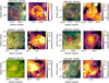 |
Fig. 5 Example newly discovered SNR candidates. MIR data are shown in the left panels and SMGPS 1.3 GHz data in the right. The symbols have the same meaning as in Fig. 1, with the candidate SNRs represented by light green circles at the centers of all panels. On the top of the panels showing SMGPS images we list our reliability classification, with I being the most reliable and III the least. Yellow scale bars at the lower left of each panel are 5′ long. |
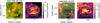 |
Fig. 6 Example unusual sources of SMGPS emission. MIR data are in the left panels (Spitzer or WISE) and SMGPS 1.3 GHz data in the right. The symbols have the same meaning as in Fig. 1, with the unusual sources represented by yellow circles at the centers of all panels. Yellow scale bars at the lower left of each panel are 5′ long. |
4.5 Comparison between the Galactic SNR, SNR candidate, and H II region populations
The areal distributions of SNRs and SNR candidates, shown in Fig. 7, are visually similar to each other. To assess whether the various samples are statistically distinct, we used a Kolmogorov- Smirnov (K-S) test, adopting p = 0.001 as the discriminating value such that statistically distinct samples will have p < 0.001.
We show the Galactic longitude distributions in the left panel of Fig. 8. Because of the increased sensitivity of the SMGPS data compared to that previously available, there are far more newly identified SNR candidates in the fourth versus the first Galactic quadrant (72 versus 28%). SNRs are more prevalent relative to H II regions between 300° < ℓ < 250°. The SNR candidate longitude distribution (including all SMGPS SNR candidates and those previously identified) is not statistically distinct from the known SNR distribution (p = 0.017).
We show the Galactic latitude distributions in the right panel of Fig. 8. The SNR candidate latitude distribution (including all SMGPS SNR candidates and those previously identified) is not statistically distinct from the known SNR distribution (p = 0.26). Least-squares fits to the binned Galactic latitude distributions of known and candidate SNRs (including both previously known and SMGPS-discovered) have full width at half maximum (FWHM) values of 0.97°, and 1.08°, respectively. The H II region distribution has a higher percentage of sources near b = 0°; its FWHM fit value is 0.75°. Measured from the standard deviation σ, however, all three samples have similar FWHM values (FWHM = 2.354σ). We find the FWHM for the samples of known SNRs, candidate SNRs, and H II regions is 1.29°, 1.25°, and 1.22°, respectively.
As shown in Fig. 9, the known and candidate SNR angular radius distributions are similar, but the SNR candidate distributions have a higher percentage of sources at lower values. A K-S test indicates that they are marginally statistically distinct (p = 0.001). Given the higher angular resolution of recent radio surveys whose data have been used to identify SNR candidates (e.g., THOR, GLOSTAR, and the SMGPS), this difference is unsurprising.
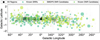 |
Fig. 7 Galactic distribution of the previously known SNRs (blue-green, from both the G22 and SNRCat samples), SMGPS SNR candidates (light green filled), and previously known SNR candidates (green open). The circles are representative of the SNR sizes. Only sources confirmed here are shown. The background is a two-dimensional histogram of the H II region density from the WISE Catalog, with higher densities indicated by darker shades. |
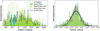 |
Fig. 8 Galactic longitude (left) and latitude (right) distributions for WISE Catalog H II regions (gray), known SNRs (blue-green, from both the G22 and SNRCat samples), SMGPS SNR candidates (light green filled), previously known SNR candidates (green open), and all SNR candidates (SMGPS-discovered and previously known combined; black open). Only sources confirmed here are shown. Curves in the right panel show leastsquares fits to the binned distributions – the gray curve for H II regions, the blue-green curve for known SNRs, and the black curve for all SNR candidates. |
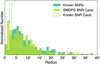 |
Fig. 9 Angular radius distributions for known SNRs (red, from both the G22 and SNRCat samples), SMGPS SNR candidates (light green filled), and previously known SNR candidates (green open). Only sources detected in SMGPS images are shown. |
4.6 Implications for the Galactic SNR population
If confirmed (i.e., with radio spectral index or polarization measurements, or with optical or X-ray searches), the 237 new SNR candidates would approximately double the known SNR population in the survey zone and would increase the total Galactic SNR population by ~80% (using the G22 number). Even if all SNR candidates are confirmed, however, there would probably be hundreds to thousands of Galactic SNRs that are yet to be identified (see Sect. 1). Future radio continuum surveys will hopefully find them.
5 Summary
Using 1.3 GHz continuum data from the SMGPS we cataloged 237 new Galactic SNR candidates. Our method identifies diffuse radio continuum emission regions lacking the MIR emission counterparts that would be seen for H II regions and planetary nebulae. All candidates lack MIR emission from known H II regions, as cataloged in the WISE Catalog. The detected candidates follow a similar areal distribution and have similar radii as the previously identified sample.
We also detect radio continuum emission and confirm the expected morphology for 201 known SNRs: 184 from Green (2022) and 30 from Ferrand & Safi-Harb (2012). We identify 2 SNRs from Green (2022) and 21 from Ferrand & Safi-Harb (2012) that we believe should be reclassified.
If our candidates prove to be true SNRs, they would approximately double the known Galactic SNR population in the surveyed region and increase the total known SNR population by ~80%. Although there is still a discrepancy between the number of known and candidate SNRs and the number of expected for a Milky Way-type galaxy, this discrepancy is now far less severe than it was a few years ago. There are now >300 Galactic SNR candidates, indicating the need for follow-up observations.
Data availability
Images and SMGPS FITS cutouts for all objects studied are hosted at https://doi.org/10.48479/0n8c-5q84. Tables A.1–A.5 are available in full at the CDS via anonymous ftp to cdsarc.cds.unistra.fr (130.79.128.5) or via https://cdsarc.cds.unistra.fr/viz-bin/cat/J/A+A/693/A247.
Acknowledgements
We thank the anonymous referee for constructive comments that increased the clarity and readability of this work. The MeerKAT telescope is operated by the South African Radio Astronomy Observatory, which is a facility of the National Research Foundation, an agency of the Department of Science and Innovation. This research has made use of the SIMBAD database, operated at CDS, Strasbourg, France. LDA thanks Cara Gillotti for her invaluable help drawing green circles. LDA and TF acknowledge support from NSF ASTR #2307176. The National Radio Astronomy Observatory is a facility of the National Science Foundation operated under cooperative agreement by Associated Universities, Inc.
Appendix A Tables available at the CDS
Previously identified SNRs from G22 (extract).
Previously identified objects from SNRCat (extract).
Previously known SNR candidates (extract).
SMGPS SNR candidates (extract).
Unusual SMGPS sources (extract).
References
- Anderson, L. D., Bania, T. M., Balser, D. S., & Rood, R. T. 2011, ApJS, 194, 32 [NASA ADS] [CrossRef] [Google Scholar]
- Anderson, L. D., Bania, T. M., Balser, D. S., et al. 2014, ApJS, 212, 1 [Google Scholar]
- Anderson, L. D., Wang, Y., Bihr, S., et al. 2017, A&A, 605, A58 [NASA ADS] [CrossRef] [EDP Sciences] [Google Scholar]
- Armentrout, W. P., Anderson, L. D., Wenger, T. V., Balser, D. S., & Bania, T. M. 2021, ApJS, 253, 23 [NASA ADS] [CrossRef] [Google Scholar]
- Ball, B. D., Kothes, R., Rosolowsky, E., et al. 2023, MNRAS, 524, 1396 [NASA ADS] [CrossRef] [Google Scholar]
- Bamba, A., Ueno, M., Koyama, K., & Yamauchi, S. 2003, ApJ, 589, 253 [NASA ADS] [CrossRef] [Google Scholar]
- Benjamin, R. A., Churchwell, E., Babler, B. L., et al. 2003, PASP, 115, 953 [Google Scholar]
- Beuther, H., Bihr, S., Rugel, M., et al. 2016, A&A, 595, A32 [NASA ADS] [CrossRef] [EDP Sciences] [Google Scholar]
- Bietenholz, M. F., & Bartel, N. 2008, MNRAS, 386, 1411 [NASA ADS] [CrossRef] [Google Scholar]
- Bietenholz, M. F., Yuan, Y., Buehler, R., Lobanov, A. P., & Blandford, R. 2015, MNRAS, 446, 205 [NASA ADS] [CrossRef] [Google Scholar]
- Bordiu, C., Riggi, F., & Cavallaro, F. 2024, A&A, submitted [Google Scholar]
- Brogan, C. L., Gelfand, J. D., Gaensler, B. M., Kassim, N. E., & Lazio, T. J. W. 2006, ApJ, 639, L25 [Google Scholar]
- Brunthaler, A., Menten, K. M., Dzib, S. A., et al. 2021, A&A, 651, A85 [EDP Sciences] [Google Scholar]
- Camilo, F., Scholz, P., Serylak, M., & et al. 2018, ApJ, 856, 180 [Google Scholar]
- Carey, S. J., Noriega-Crespo, A., Mizuno, D. R., et al. 2009, PASP, 121, 76 [Google Scholar]
- Churchwell, E., Babler, B. L., Meade, M. R., et al. 2009, PASP, 121, 213 [Google Scholar]
- Cohen, M., & Green, A. J. 2001, MNRAS, 325, 531 [NASA ADS] [CrossRef] [Google Scholar]
- Cotton, W. D., Kothes, R., Camilo, F., et al. 2024, ApJS, 270, 21 [NASA ADS] [CrossRef] [Google Scholar]
- de Avillez, M. A., & Breitschwerdt, D. 2005, A&A, 436, 585 [NASA ADS] [CrossRef] [EDP Sciences] [Google Scholar]
- Dokara, R., Roy, N., Beuther, H., et al. 2018, ApJ, 866, 61 [Google Scholar]
- Dokara, R., Brunthaler, A., Menten, K. M., et al. 2021, A&A, 651, A86 [EDP Sciences] [Google Scholar]
- Driessen, L. N., Domček, V., Vink, J., et al. 2018, ApJ, 860, 133 [Google Scholar]
- Dubner, G., & Giacani, E. 2015, A&A Rev., 23, 3 [NASA ADS] [CrossRef] [Google Scholar]
- Faucher-Giguère, C.-A., Quataert, E., & Hopkins, P. F. 2013, MNRAS, 433, 1970 [Google Scholar]
- Ferrand, G., & Safi-Harb, S. 2012, Adv. Space Res., 49, 1313 [Google Scholar]
- Gaensler, B. M., Slane, P. O., Gotthelf, E. V., & Vasisht, G. 2001, ApJ, 559, 963 [NASA ADS] [CrossRef] [Google Scholar]
- Girichidis, P., Walch, S., Naab, T., et al. 2016, MNRAS, 456, 3432 [NASA ADS] [CrossRef] [Google Scholar]
- Goedhart, S., Cotton, W. D., Camilo, F., et al. 2024, MNRAS, 531, 649 [CrossRef] [Google Scholar]
- Gonçalves, D. P., Noriega-Crespo, A., Paladini, R., Martin, P. G., & Carey, S. J. 2011, AJ, 142, 47 [CrossRef] [Google Scholar]
- Green, D. A. 2004, Bull. Astron. Soc. India, 32, 335 [NASA ADS] [Google Scholar]
- Green, D. A. 2014, Bull. Astron. Soc. India, 42, 47 [NASA ADS] [Google Scholar]
- Green, D. A. 2015, MNRAS, 454, 1517 [NASA ADS] [CrossRef] [Google Scholar]
- Green, D. A. 2022, A Catalogue Galactic Supernova Remnants (2022 December version) [Google Scholar]
- Green, A. J., Reeves, S. N., & Murphy, T. 2014, PASA, 31, e042 [Google Scholar]
- Helfand, D. J., Becker, R. H., White, R. L., Fallon, A., & Tuttle, S. 2006, AJ, 131, 2525 [Google Scholar]
- Hurley-Walker, N., Gaensler, B. M., Leahy, D. A., et al. 2019, PASA, 36, e048 [NASA ADS] [CrossRef] [Google Scholar]
- Jonas, J., & MeerKAT Team. 2016, in MeerKAT Science: On the Pathway to the SKA, 1 [Google Scholar]
- Joung, M. R., Mac Low, M.-M., & Bryan, G. L. 2009, ApJ, 704, 137 [NASA ADS] [CrossRef] [Google Scholar]
- Kaplan, D. L., Kulkarni, S. R., Frail, D. A., & van Kerkwijk, M. H. 2002, ApJ, 566, 378 [NASA ADS] [CrossRef] [Google Scholar]
- Lazarević, S., Filipović, M. D., Koribalski, B. S., et al. 2024, RNAAS, 8, 107 [Google Scholar]
- Li, Z., Wheeler, J. C., Bash, F. N., & Jefferys, W. H. 1991, ApJ, 378, 93 [Google Scholar]
- Loru, S., Ingllinera, A., Umana, G., et al. 2024, A&A, 692, A193 [NASA ADS] [CrossRef] [EDP Sciences] [Google Scholar]
- Mauch, T., Cotton, W., Condon, J., & et al. 2020, ApJ, 888, 61 [NASA ADS] [CrossRef] [Google Scholar]
- Maxted, N. I., Filipović, M. D., Hurley-Walker, N., et al. 2019, ApJ, 885, 129 [NASA ADS] [CrossRef] [Google Scholar]
- Ostriker, E. C., & Shetty, R. 2011, ApJ, 731, 41 [Google Scholar]
- Ostriker, E. C., McKee, C. F., & Leroy, A. K. 2010, ApJ, 721, 975 [CrossRef] [Google Scholar]
- Padoan, P., Pan, L., Haugbølle, T., & Nordlund, Å. 2016, ApJ, 822, 11 [NASA ADS] [CrossRef] [Google Scholar]
- Pinheiro Gonçalves, D., Noriega-Crespo, A., Paladini, R., Martin, P. G., & Carey, S. J. 2011, AJ, 142, 47 [Google Scholar]
- Ranasinghe, S., & Leahy, D. 2022, ApJ, 940, 63 [NASA ADS] [CrossRef] [Google Scholar]
- Reach, W. T., Rho, J., Tappe, A., et al. 2006, AJ, 131, 1479 [NASA ADS] [CrossRef] [Google Scholar]
- Sidorin, V., Douglas, K. A., Palouš, J., Wünsch, R., & Ehlerová, S. 2014, A&A, 565, A6 [NASA ADS] [CrossRef] [EDP Sciences] [Google Scholar]
- Smeaton, Z. J., Filipović, M. D., Lazarević, S., et al. 2024, MNRAS, 534, 2918 [Google Scholar]
- Stil, J. M., Taylor, A. R., Dickey, J. M., et al. 2006, AJ, 132, 1158 [NASA ADS] [CrossRef] [Google Scholar]
- Supan, L., Castelletti, G., Peters, W. M., & Kassim, N. E. 2018, A&A, 616, A98 [NASA ADS] [CrossRef] [EDP Sciences] [Google Scholar]
- Sushch, I., Oya, I., Schwanke, U., Johnston, S., & Dalton, M. L. 2017, A&A, 605, A115 [NASA ADS] [CrossRef] [EDP Sciences] [Google Scholar]
- Tammann, G. A., Loeffler, W., & Schroeder, A. 1994, ApJS, 92, 487 [Google Scholar]
- Trushkin, S. A. 2001, in ESA Special Publication, 459, Exploring the GammaRay Universe, eds. A. Gimenez, V. Reglero, & C. Winkler, 109 [NASA ADS] [Google Scholar]
- Voit, G. M. 1992, MNRAS, 258, 841 [NASA ADS] [CrossRef] [Google Scholar]
- Weiler, K. W., & Sramek, R. A. 1988, ARA&A, 26, 295 [NASA ADS] [CrossRef] [Google Scholar]
- Whiteoak, J. B. Z., & Green, A. J. 1996, A&AS, 118, 329 [NASA ADS] [CrossRef] [EDP Sciences] [Google Scholar]
- Wright, E. L., Eisenhardt, P. R. M., Mainzer, A. K., et al. 2010, AJ, 140, 1868 [Google Scholar]
The most recent published version is that of Green (2014); we used the online version.
We follow the convention that positive values of α indicate increasing flux densities with frequency.
Data can be found here: https://doi.org/10.48479/3wfd-e270. When using DR1 products, Goedhart et al. (2024) should be cited, and the MeerKAT telescope acknowledgement included.
Note added in proof: one of our SNR candidates, G308.730+01.380, was identified in Lazarević et al. (2024) as SNR candidate G308.73+1.38.
See Brogan et al. (2006) and Hurley-Walker et al. (2019), who used the same nomenclature with slightly different definitions.
Note added in proof: one of our unusual sources, G329.877−00.458, was identified in Smeaton et al. (2024) as SNR G329.9−0.5.
All Tables
All Figures
|
Fig. 1 Example field centered at (ℓ, b) = (324.0°, −0.2°). Top: Spitzer three-color data, with MIPSGAL 24 µm data in red, GLIMPSE 8.0 µm data in green, and GLIMPSE 3.6 µm data in blue. Middle: 1.3 GHz SMGPS data. Bottom: 1.3 GHz SMGPS data in red, MIPSGAL 24 µm data in green, and GLIMPSE 8.0 µm data in blue. White circles show HII regions from the WISE Catalog (Sect. 2.3), blue-green circles previously known SNRs (Sect. 4.1), green circles previously known SNR candidates (Sect. 4.2), light green circles SNR candidates newly identified here (Sect. 4.3), and yellow circles “unusual” sources (Sect. 4.4). Although there are no examples in this field, in subsequent figures we show misidentified or undetected SNRs and SNR candidates with dashed circles. |
| In the text | |
|
Fig. 2 Objects from the G22 catalog. MIR data (Spitzer or WISE) are shown in the left panels and SMGPS 1.3 GHz data in the right. The symbols have the same meaning as in Fig. 1, with the G22 SNRs represented by blue-green circles at the centers of all panels. Cyan scale bars at the lower left of each panel are 5′ long. |
| In the text | |
|
Fig. 3 Objects from the G22 catalog split into two entries, G337.0−0.1* and G337.0−0.1. MIR data are shown in the left panels and SMGPS 1.3 GHz data in the right. The symbols have the same meaning as in Fig. 1, with the G22 SNRs represented by blue-green circles at the centers of all panels. Yellow scale bars at the lower left of each panel are 5′ long. |
| In the text | |
|
Fig. 4 Objects from the G22 catalog that are unlikely to be true SNRs. MIR data are in the left panels (Spitzer or WISE) and SMGPS 1.3 GHz data in the right. The symbols have the same meaning as in Fig. 1, with the G22 SNRs indicated by dashed blue-green circles at the centers of all panels. Yellow scale bars at the lower left of each panel are 5′ long. |
| In the text | |
|
Fig. 5 Example newly discovered SNR candidates. MIR data are shown in the left panels and SMGPS 1.3 GHz data in the right. The symbols have the same meaning as in Fig. 1, with the candidate SNRs represented by light green circles at the centers of all panels. On the top of the panels showing SMGPS images we list our reliability classification, with I being the most reliable and III the least. Yellow scale bars at the lower left of each panel are 5′ long. |
| In the text | |
|
Fig. 6 Example unusual sources of SMGPS emission. MIR data are in the left panels (Spitzer or WISE) and SMGPS 1.3 GHz data in the right. The symbols have the same meaning as in Fig. 1, with the unusual sources represented by yellow circles at the centers of all panels. Yellow scale bars at the lower left of each panel are 5′ long. |
| In the text | |
|
Fig. 7 Galactic distribution of the previously known SNRs (blue-green, from both the G22 and SNRCat samples), SMGPS SNR candidates (light green filled), and previously known SNR candidates (green open). The circles are representative of the SNR sizes. Only sources confirmed here are shown. The background is a two-dimensional histogram of the H II region density from the WISE Catalog, with higher densities indicated by darker shades. |
| In the text | |
|
Fig. 8 Galactic longitude (left) and latitude (right) distributions for WISE Catalog H II regions (gray), known SNRs (blue-green, from both the G22 and SNRCat samples), SMGPS SNR candidates (light green filled), previously known SNR candidates (green open), and all SNR candidates (SMGPS-discovered and previously known combined; black open). Only sources confirmed here are shown. Curves in the right panel show leastsquares fits to the binned distributions – the gray curve for H II regions, the blue-green curve for known SNRs, and the black curve for all SNR candidates. |
| In the text | |
|
Fig. 9 Angular radius distributions for known SNRs (red, from both the G22 and SNRCat samples), SMGPS SNR candidates (light green filled), and previously known SNR candidates (green open). Only sources detected in SMGPS images are shown. |
| In the text | |
Current usage metrics show cumulative count of Article Views (full-text article views including HTML views, PDF and ePub downloads, according to the available data) and Abstracts Views on Vision4Press platform.
Data correspond to usage on the plateform after 2015. The current usage metrics is available 48-96 hours after online publication and is updated daily on week days.
Initial download of the metrics may take a while.