| Issue |
A&A
Volume 605, September 2017
|
|
|---|---|---|
| Article Number | A61 | |
| Number of page(s) | 11 | |
| Section | Interstellar and circumstellar matter | |
| DOI | https://doi.org/10.1051/0004-6361/201730575 | |
| Published online | 11 September 2017 | |
Multiplicity and disks within the high-mass core NGC 7538IRS1
Resolving cm line and continuum emission at ~0.06″ × 0.05″ resolution⋆
1 Max Planck Institute for Astronomy, Königstuhl 17, 69117 Heidelberg, Germany
e-mail: This email address is being protected from spambots. You need JavaScript enabled to view it.
2 Max Planck Institute for Extraterrestrial Physics, Giessenbachstrasse 1, 85748 Garching, Germany
Received: 7 February 2017
Accepted: 9 May 2017
Abstract
Context. High-mass stars have a high degree of multiplicity and most likely form via disk accretion processes. The detailed physics of the binary and disk formation are still poorly constrained.
Aims. We seek to resolve the central substructures of the prototypical high-mass star-forming region NGC 7538IRS1 at the highest possible spatial resolution in line and continuum emission to investigate the protostellar environment and kinematics.
Methods. Using the Karl G. Jansky Very Large Array (VLA) in its most extended configuration at ~24 GHz has allowed us to study the NH3 and thermal CH3OH emission and absorption as well as the cm continuum emission at an unprecedented spatial resolution of 0.06″ × 0.05″, corresponding to a linear resolution of ~150 AU at a distance of 2.7 kpc.
Results. A comparison of these new cm continuum data with previous VLA observations from 23 yr ago reveals no recognizable proper motions. If the emission were caused by a protostellar jet, proper motion signatures should have been easily identified. In combination with the high spectral indices S ∝ να (α between 1 and 2), this allows us to conclude that the continuum emission is from two hypercompact Hii regions separated in projection by about 430 AU. The NH3 spectral line data reveal a common rotating envelope indicating a bound high-mass binary system. In addition to this, the thermal CH3OH data show two separate velocity gradients across the two hypercompact Hii regions. This indicates two disk-like structures within the same rotating circumbinary envelope. Disk and envelope structures are inclined by ~33 °, which can be explained by initially varying angular momentum distributions within the natal, turbulent cloud.
Conclusions. Studying high-mass star formation at sub-0.1″ resolution allows us to isolate multiple sources as well as to separate circumbinary from disk-like rotating structures. These data show also the limitations in molecular line studies in investigating the disk kinematics when the central source is already ionizing a hypercompact Hii region. Recombination line studies will be required for sources such as NGC 7538IRS1 to investigate the gas kinematics even closer to the protostars.
Key words: stars: formation / stars: massive / stars: individual: NGC 7538IRS1 / stars: rotation / instrumentation: interferometers
The data presented in this article are only available at the CDS via anonymous ftp to cdsarc.u-strasbg.fr (130.79.128.5) or via http://cdsarc.u-strasbg.fr/viz-bin/qcat?J/A+A/605/A61
© ESO, 2017
1. Introduction
The formation processes leading to the most massive stars are still puzzling in many ways. While there is a clear consensus that high-mass stars shape the interstellar medium, whole clusters, and even entire galaxies, questions related to the physical processes at early evolutionary stages, in particular associated with the fragmentation processes of young, dense, and rotating cores, formation of multiple entities, and embedded accretion disks, are still poorly explored (e.g., Beuther et al. 2007a; Zinnecker & Yorke 2007; Tan et al. 2014; Beltrán & de Wit 2016).
How do massive accretion disks form and what are their properties? These are central questions for high-mass star formation research (e.g., Henning et al. 2000; Kratter & Matzner 2006; Beuther et al. 2009; Cesaroni et al. 2007; Vaidya et al. 2009; Kraus et al. 2010, 2017; Beltrán et al. 2011; Ilee et al. 2013; Boley et al. 2013, 2016; Sánchez-Monge et al. 2014; Johnston et al. 2015). The main indirect evidence stems from observations of massive and collimated outflows that are qualitatively similar to low-mass jets (e.g., Beuther et al. 2002; Zhang et al. 2005; Arce et al. 2007; López-Sepulcre et al. 2009; Duarte-Cabral et al. 2013). Such jet-like outflows are best explained via magneto-centrifugal acceleration from an accretion disk and subsequent Lorentz collimation. Radiation (M)HD simulations of massive collapsing cores produce accretion disks as well (e.g., Yorke & Sonnhalter 2002; Krumholz et al. 2009; Kuiper et al. 2010, 2011; Kuiper & Yorke 2013; Peters et al. 2010; Commerçon et al. 2011). Are massive disks similar to their low-mass counterparts, hence dominated by the protostar and Keplerian rotation or are they self-gravitating non-Keplerian entities (e.g., Sánchez-Monge et al. 2013; Cesaroni et al. 2007)? The answer may be a small inner Keplerian accretion disk that is fed from a larger-scale non-Keplerian structure (toroid or pseudo-disk). This picture is supported by analytic and numeric models with Keplerian disks growing with time from the infalling rotating structure (e.g., Stahler & Palla 2005; Kuiper et al. 2011). The transition from molecular to ionized infall is an additional important characteristic (e.g., Keto 2002, 2003; Klaassen et al. 2009, 2013). While indirect evidence for massive disks is very strong, direct observations are still sparse (see AFGL4176 as one of the best recent examples; Johnston et al. 2015, of G11.92-0.61 by Ilee et al. 2016). This discrepancy is mainly due to the clustered mode of massive star formation at large distances. High spatial resolution is crucial to disentangle these structures.
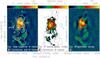 |
Fig. 1 Centimeter continuum emission from NGC 7538IRS1. The left panel shows in color scale the new 1.2 cm continuum data imaged using only baselines between 10 and 37 km, achieving a spatial resolution of 0.06″ × 0.05″. The contours present for comparison the old VLA data from 1992 discussed previously in Gaume et al. (1995a), Sandell et al. (2009), Moscadelli & Goddi (2014), and Goddi et al. (2015) starting at the 4σ contour and continuing in 8σ intervals (1σ ~ 0.05 mJy beam-1). The two stars indicate the CH3OH maser positions by Moscadelli & Goddi (2014); see Sect. 3.1 for more details. The middle panel shows in color the spectral index map derived from the new full dataset with robust weighting −2 and the contours show the corresponding continuum image using all data at a resolution of 0.07″ × 0.05″. The contour levels start at a 4σ levels of 0.16 mJy beam-1 and continue in coarser 32σ steps. The right panel again shows the new 0.06″ × 0.05″ data, now converted in the Rayleigh-Jeans approximation to brightness temperature. |
What are the fragmentation properties of massive gas clumps during the formation of high-mass stars and their surrounding clusters? High-mass stars form in clusters with a high degree of multiplicity, and Chini et al. (2012) argue that this multiplicity likely stems from the formation processes (see also Peter et al. 2012). Peter et al. (2012) find companion separations between 400 and several thousand AU, stressing the necessity of high spatial resolution, Furthermore, Sana et al. (2012) infer that multiple system interactions dominate the evolution of massive stars. Interferometer studies have revealed that most high-mass star-forming regions fragment into multiple objects, suggesting that massive monolithic cores larger than several 1000 AU are rare, however, the degree of fragmentation varies (e.g., Cesaroni et al. 2005; Beuther et al. 2007b, 2012; Zhang et al. 2009; Bontemps et al. 2010; Wang et al. 2011; Rodón et al. 2012; Palau et al. 2013; Sánchez-Monge et al. 2014; Johnston et al. 2015). Even regions that remain single continuum sources down to arcsec resolution, mostly fragment on even smaller scales.
A particularly revealing example is the famous high-mass star-forming region NGC 7538IRS1. At a distance of ~2.7 kpc (Moscadelli et al. 2009), the luminosity of the central energy source is estimated to stem from a 30 M⊙ O6 star (e.g., Willner 1976; Gaume et al. 1995a; Moscadelli et al. 2009). The strong emission of this source from near- to mid-infrared wavelengths to the cm- and mm-regime has made it a famous high-mass protostar for over several decades; a summary of the literature can be found in Beuther et al. (2012). The recent 0.2″ observations at submm wavelengths with the Northern Extended Millimeter Array (NOEMA) revealed fragmentation of the envelope, however, these observations did not allow us to identify a Keplerian accretion disk (Beuther et al. 2013, see also high-resolution data by Zhu et al. 2013). Most likely, such a Keplerian structure is hidden on still smaller scales below 500 AU (e.g., Krumholz et al. 2007; Kuiper et al. 2010, 2011). Furthermore, this region reveals two cm continuum sources at approximately 0.2″ separation that may either be two hypercompact Hii region or an ionized jet (Gaume et al. 1995b; Sandell et al. 2009; Moscadelli & Goddi 2014; Goddi et al. 2015), where the association of the potential ionized jet with the molecular outflow is debated (Knez et al. 2009; Beuther et al. 2013).
Parameters of main spectral lines.
2. Observations
We observed NGC 7538IRS1 on July 21, 2015, during a four hour track with the Karl G. Jansky Very Large Array (VLA) in its most extended A-configuration (baselines extending out to 37 km). The proposal ID is 15A-115. With the flexible VLA correlator we covered many spectral lines and the cm continuum emission in the radio K band. Specifically we covered seven NH3 inversion lines, seven CH3OH lines, and two Hα recombination lines. Line parameters are given in Table 1. The following analysis concentrates on the cm continuum, NH3, and CH3OH emission. Although the recombination lines are detected, the emission is comparably weak and is not discussed further here. The intrinsic spectral resolution for the molecular line data varied between 15.625 and 31.25 kHz, corresponding to a velocity resolution of ~0.19 and ~0.38 km s-1 at the given frequencies, respectively (Table 1). Since this region is very strong in absorption and emission, we reduced almost all lines at the native correlator resolution. Only the three lowest energy CH3OH lines – located within a single spectral window – were reduced separately with 0.4 km s-1 resolution. To create the continuum image, 16 spectral windows with a width of 112 MHz each between 23.6 and 25.8 GHz were combined.
The flux and bandpass were calibrated with the two strong quasars 3C 48 and J0319+4130 (also known as 3C 84), respectively. The phase and amplitude gain calibration for these long baselines requires comparatively fast switching between the target source and the gain calibrator J2339+6010. Our loop typically stayed 1 min 50 s on source and 1 min 20 s on the gain calibrator. We visited the source during the 4 h track 58 times assuring an excellent uv coverage. The phase center of the VLA for our target source NGC 7538IRS1 was RA (J2000.0) 23:13:45.36 and Dec (J2000.0) +61:28:10.55. The data calibration was conducted with the VLA pipeline 1.3.1 in CASA 4.2.2. All solutions were carefully checked, and the bandpass for the NH3(1, 1) line was bad during half of the track. Flagging this second half for this one spectral window and then rerunning the pipeline gave excellent results.
Further imaging and analysis of the data was also conducted in CASA. The continuum data were imaged with two different approaches: once using all data with a robust weighting value of –2, and once excluding baselines of the inner 10 km (baselines covered between 10 and 37 km) to even improve the spatial resolution. While the normal robust –2 dataset with all data resulting in a beam of 0.07″ × 0.05″ (PA −25°) was better suited for studying the spectral index, the highest-spatial-resolution image with restricted baseline range and a spatial resolution of 0.06″ × 0.05″ (PA −32°) was used for morphological comparison. The largest scales typically recoverable with the VLA at this frequency in the A-array are ~2.4″. The 1σ rms for both images is ~0.05 mJy beam-1. The molecular line data were all imaged with a robust weighting scheme and a robust value of 0. Just the NH3(1, 1) data were also imaged in natural weighting (robust value 2) for comparison (see Sect. 3.2). While the naturally weighted NH3(1, 1) image has a beam of 0.11″ × 0.09″ (PA −31°), the other images with robust weighting 0 have a synthesized beam of 0.08″ × 0.06″ (PA varying between −28° and −30°). The 1σ rms measured in an emission- and absorption-free channel varies between 2.1 and 3.9 mJy beam-1.
3. Results
3.1. Centimeter continuum emission
The double-peaked structure of the cm continuum emission presented in Gaume et al. (1995a), Sandell et al. (2009), and Moscadelli & Goddi (2014) can be interpreted in a two ways: On the one hand, this structure may be two separate protostellar sources, whereas, on the other hand, the double-peaked structure could also be part of one underlying jet. Our new data now allow us to address this question with two approaches: (a) search for proper motions with a time baseline from December 1992 (Gaume et al. 1995a; observed in the same configuration and wavelength as our new data) and our new data from July 2015 presented here. And (b) an analysis of the spectral index based on the broad bandpass of the new data. Figure 1 presents an overlay of the old and new data as well as a spectral index map. The spectral index map was derived from all 16 continuum windows between 23.6 and 25.8 GHz in CASA within the clean task using higher order Taylor terms (parameter nterm = 2) to model the frequency dependence of the sky emission. The spectral index map is computed as the ratio of the first two Taylor terms. This task also computes an error map of the spectral index treating the Taylor-coefficient residuals as errors and propagating them through the spectral index determination. The spectral index map in Fig. 1 is clipped for errors larger than 0.4.
Continuum source parameters.
To search for proper motions, the highest possible positional accuracy is required. Table 2 presents the peak positions and peak fluxes at 24.6 GHz. When investigating the data for NGC 7538IRS1 in detail, two issues arose. First, the positional accuracy of the phase calibrator was incorrect by ΔRA ~ 0.01″ and ΔDec ~ 0.16″ (Moscadelli & Goddi 2014; Goddi et al. 2015). We corrected for this positional shift after the imaging process. Furthermore, Moscadelli et al. (2009) and Moscadelli & Goddi (2014) inferred proper motions for the region of –2.45 mas yr-1/–2.45 mas yr-1 from CH3OH maser observations at 12 GHz. For the 22.58 yr time difference between the two observational epochs, this corresponds to a shift of ~0.055″ in RA and Dec, respectively. To get the 1992 and 2015 data into the same framework, we shifted the 1992 data according to these proper motions. Figure 1 takes both shifts into account. Furthermore, we show the central positions of the CH3OH maser groups IRS1a and IRS1b as presented in Fig. 11 of Moscadelli & Goddi (2014). Since the maser positions in Moscadelli & Goddi (2014) are from 2005, we also have to apply the above proper motion shift to these for comparison. The final CH3OH maser group positions plotted in this paper are IRS1a: RA (J2000.0) 23:13:45.368 and Dec (J2000.0) 61:28:10.286 and IRS1b: RA (J2000.0) 23:13:45.358 and Dec (J2000.0) 61:28:10.486.
We find that the overall structure of the two central peaks associated with the two CH3OH maser positions have not moved significantly within the spatial resolution and uncertainties of the two observational datasets. The northern source cm1 is elongated in northeastern direction, which is already visible in the old data. No positional shift can be identified for the northern of the two main peaks cm1, whereas the second main source cm2 exhibits a tiny shift of ~0.025″. However, this is less than half of the synthesized beam and we refrain from further interpretation of that apparently very small shift. The additional emission feature ~0.4′′ to the south appears to have shifted slightly in southeastern direction. Since we are mainly interested in the two main emission peaks cm1 and cm2, we do not further analyze the separate southern structure.
At the given distance of 2.7 kpc, our approximate average spatial resolution element 0.055″ corresponds to a linear resolution of ~150 AU. Assuming a jet velocity of ~250 km s-1 with an inclination angle of 45°, the 23 yr time baseline between the two observational epochs would still result in proper motions of ~857 AU, corresponding in an angular shift of ~0.32′′, which is well resolvable by our observations. Although the inclination angle is unknown, jets may be even faster (Martí et al. 1998; Frank et al. 2014; Guzmán et al. 2016) and hence these data are strong evidence that a jet is unlikely the underlying cause for the cm continuum emission.
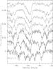 |
Fig. 2 NH3 example spectra extracted toward the northern cm continuum peak position. The spectra are shifted of the y-axis for presentation purposes. All lines are labeled. |
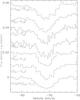 |
Fig. 3 CH3OH example spectra extracted toward the northern cm continuum peak position. The spectra are shifted of the y-axis for presentation purposes. All lines are labeled. |
Regarding the spectral index S ∝ να, for a hypercompact Hii region α can vary between –0.1 for optically thin to +2 for optically thick emission. While large Hii regions are typically in the optically thin regime at the given frequency around 24 GHz, a hypercompact Hii region such as NGC 7538IRS1 can easily be in the (partly) optically thick regime (e.g., Franco et al. 2000). For comparison, while ionized jets theoretically can cover the same spectral index regime, typical emission from an ionized jet has rather a spectral index α around +0.6 (e.g., Reynolds 1986; Purser et al. 2016). The observed spectral index α shown in Figure 1 varies largely between 1 and 2. Therefore, the spectral index analysis of NGC 7538IRS1 also indicates that the cm continuum emission is not caused by an ionized jet but more likely is dominated by a hypercompact Hii region(s).
With the high optical depth indicated by the spectral index, converting the cm continuum fluxes in the Rayleigh-Jeans limit to brightness temperatures additionally gives a hint about the temperatures of the ionized gas. Figure 1 (right panel) shows that the brightness temperatures of the inner region vary between approximately 2000 and 4900 K. These can be considered as lower limits for the ionized gas temperatures because the spectral index as a proxy of the optical depth varies throughout the region.
Combining the multiepoch and multiwavelength analysis above, the central double-lobe cm continuum emission in NGC 7538IRS1 is most likely emitted by at least two embedded protostars within their associated hypercompact Hii regions.
3.2. NH3 and CH3OH
At this high spatial resolution and with the given very strong continuum emission, all molecular line features are only observed in absorption against the continuum sources. Figures 2 and 3 show example spectra of all NH3 and CH3OH lines extracted toward the northern cm continuum peak position. For NH3 the hyperfine structure is detected for all lines. The integrated, 1st and 2nd moment maps and the position-velocity diagrams discussed below (Figs. 4 to 8) were created after inverting the data (simply multiplying by –1) because the corresponding algorithms in CASA only work on positive data. This inversion does not affect the kinematic signatures at all. The excitation temperatures El/k and the critical densities calculated as ncrit = A/C (with the Einstein coefficient A and the collision rate C from the LAMBDA database; Schöier et al. 2005) are given in Table 1 as well. While NH3 covers an excitation range between 22 and 537 K, this is slightly smaller for CH3OH between 28 and 149 K. However, while the critical densities ncrit for NH3 are around 2000 cm-3, they are more than an order of magnitude larger for CH3OH around a few times 104 cm-3. In addition to this, the chosen J2−J1 25 GHz transitions of CH3OH have been found to emit as masers in several high-mass star-forming regions (e.g., Menten et al. 1986; Voronkov et al. 2007; Brogan et al. 2012). These masers are likely collisionly excited (e.g., Sobolev & Strelnitskii 1983) and thus form its own subgroup of methanol Class I maser (e.g., Leurini et al. 2016). Compared to other types of Class I masers, they need higher gas volume densities for the population inversion to occur (n > 106 cm-3; e.g., Sobolev et al. 1998; Leurini et al. 2016). The fact that we see the 25 GHz transitions in absorption might be an indication that the majority of the methanol in NGC 7538 IRS1 relevant for our absorption is residing in somewhat lower density gas.
Figure 4 presents the 1st moment maps (intensity-weighted velocities) of the NH3 inversion lines from (1, 1) to (7, 7). The first two maps of the (1, 1) transition are produced with different weighting schemes (natural weighting and robust weighting 0) recovering different spatial structures. While the naturally weighted NH3(1, 1) shows a bit more extended emission, one sees a larger scale velocity gradient approximately in east-west direction. In comparison to that, the higher resolution (robust weighting 0) image rather reveals a velocity gradient in northeast-southwest direction, which is consistent with previous findings by Beuther et al. (2012, 2013), Moscadelli & Goddi (2014), and Goddi et al. (2015). Since we are mainly interested in the kinematics of the innermost central sources we concentrate in the following on the higher resolution data. All other transitions are also presented in this higher resolution imaging mode (robust weighting 0).
Interestingly, all seven NH3 inversion lines with excitation levels El/k between 22 and 537 K (Table 1) exhibit almost the same kinematic structure of the central core with one velocity gradient in approximately northeast-southwest direction, but without any differentiation between the two continuum sources seen in the overlayed contours (Fig. 4). These NH3 velocity structures appear similar to the previous findings for the rotational structure of the rotating envelope by Beuther et al. (2013) and Goddi et al. (2015). Performing spectral cuts across the main velocity gradient direction (NH3(7, 7) panel in Fig. 4 indicates the exact orientation), Fig. 5 presents the corresponding position-velocity diagrams. The two panels corresponding to the (1, 1) inversion lines exhibit three features because of the close-in frequency-space hyperfine structure. The other six lines only show the central strong hyperfine component. This velocity gradient is almost linear across the source. It does not show any hint of Keplerian motion but resembles more a solid-body rotation diagram.
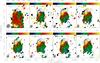 |
Fig. 4 Color-scale presents the 1st moment maps (intensity-weighted velocities) of the NH3 inversion transitions from (1, 1) to (7, 7) as indicated in each panel. The first two left panels show the data for the NH3(1, 1) line with different weighting schemes (natural weighting and robust weighting, which is a hybrid between natural and uniform weighting). The other NH3 lines are always presented with robust weighting 0. The 1st moment maps are clipped at a ~4σ level. The contours show in all panels the 1.2 cm continuum emission in levels of 8% to 98% of the peak emission (7.4 mJy beam-1). The two stars indicate the CH3OH maser positions by Moscadelli & Goddi (2014). The line in the bottom right panel indicates the position-velocity cut shown below. |
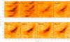 |
Fig. 5 Position-velocity diagrams for the different NH3 inversion lines as indicated in each panel. The direction of the cut is shown in Fig. 4. The top left and top 2nd panels show this cut for natural and robust weighting for the NH3(1, 1) lines, respectively. All other cuts are carried out for the robust weighting case. |
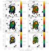 |
Fig. 6 Integrated (left) and 2nd moment (right) maps (intensity-weighted velocity dispersion) for two NH3 and one CH3OH line as indicated in each panel. The integration ranges for NH3(3, 3), (7, 7) and CH3OH(102,8−101,9) are [–68, –50] km s-1, [–65, –50] km s-1 and [–65, –53] km s-1, respectively. The contours show in all panels the 1.2 cm continuum emission in levels of 8% to 98% of the peak emission (7.4 mJy beam-1). The two stars indicate the CH3OH maser positions by Moscadelli & Goddi (2014). The synthesized beams are shown in the bottom left of each panel. |
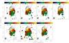 |
Fig. 7 Color-scale presents the 1st moment maps (intensity-weighted velocities) of the CH3OH lines as shown in each panel. The contours show in all panels the 1.2 cm continuum emission in levels of 8% to 98% of the peak emission (7.4 mJy beam-1). The two stars indicate the CH3OH maser positions by Moscadelli & Goddi (2014). The two lines in the bottom right panel indicate the cuts for the position-velocity diagrams shown below. |
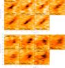 |
Fig. 8 Position-velocity diagrams for the different CH3OH lines as indicated in each panel. The top seven panels belong to the northern cut and the bottom seven panels to the southern cut shown in Fig. 7. All cuts are performed for the robust weighting 0 case. |
For comparison, Fig. 6 presents also the integrated absorption and the 2nd moment maps (intensity-weighted velocity dispersion) for two selected NH3 and one CH3OH lines. The spatial structure of these integrated and velocity dispersion maps does not reflect the overall velocity gradient seen in NH3, but all maps are double-peaked toward the two cm continuum peak positions. This shows that the largest gas column densities and strongest line broadening are indeed associated with the two main protostellar condensations. The fact that NH3 exhibits two centers of line broadening, in spite of only a single larger scale velocity gradient, indicates the potential existence of two smaller scale embedded rotating structures.
The important new information now stems from the thermal CH3OH absorption data. Similar to NH3, for CH3OH we also present the 1st moment maps and position-velocity diagrams in Figs. 7 and 8. While the CH3OH 1st moment maps also exhibit the general trend of velocities from the northeast to the southwest, the data show a clear structural change between the northern and southern continuum source. With these data one can depict for all lines with excitation levels between 28 and 149 K (Table 1) one velocity gradient across the northern continuum source and one velocity gradient across the southern continuum source. These two velocity gradients are almost parallel in the east-northeast to west-southwest direction. While we identify these velocity gradients in thermal CH3OH absorption, the previously studied CH3OH class II masers also show velocity gradients approximately in the east-west direction (Moscadelli & Goddi 2014). Although the angles derived from the maser and thermal absorption are not exactly the same, they are both approximately in east-west direction and both have the same orientation with respect to the blue- and redshifted structure. Hence, while the maser and thermal emission and absorption trace different spatial scales, both appear to stem from the same rotating structures.
Figures 8 presents the corresponding position-velocity cuts along the two axes outlined in the bottom right panel of Fig. 7. For both regions we identify clear velocity gradients across the sources, however, in both cases again without any Keplerian signature. The underlying physical reasons for these kinematic signatures are discussed in Sect. 4.2.
While the measured velocity dispersion of the two NH3 lines varies only a bit, the velocity dispersion of CH3OH is considerably narrower (Fig. 6). Only the overlap region between the two continuum peaks shows a larger velocity dispersion, but this can be attributed to beam smearing effects between the two peak positions. Inspecting individual absorption spectra against the main northern continuum peak position (Fig. 9), the spectral profiles show why the measured line widths in NH3 and CH3OH are different. While the peak and redshifted side of the absorption spectra are similar, NH3 shows a pronounced blueshifted wing. In absorption spectra that is clear sign for outflowing gas. Because the critical density of NH3 is an order of magnitude lower than that of CH3OH (Table 1), it appears that NH3 also traces outflowing gas of within the envelope whereas the CH3OH signatures are more dominated by the rotating disk-like structures.
4. Discussion
4.1. Fragmentation and multiplicity
The high-mass star-forming region NGC 7538IRS1 is intriguing because it does not show significant fragmentation signatures in the cold dust and gas emission at (sub)mm wavelengths. At ~0.3 resolution and 1.3 mm wavelength, Beuther et al. (2012) still identified only a single source, whereas then at ~0.2″ resolution and 843 μm wavelength first fragmentation signatures of the innermost rotating structure could be identified (Beuther et al. 2013). Our new (non-)proper motion analysis, spectral index study and the kinematic signatures in CH3OH clearly confirm that at least two very young protostars are embedded within the innermost core. The elongation in northeastern direction of the northern source cm1 may harbor further subsources. However, this elongation may also be due to an underlying ionized disk-like structure since it is approximately aligned with the CH3OH velocity gradient. The projected separation of the two main protostars cm1 and cm2 is ~0.16″ or ~430 AU. Since the two sources are embedded in a large-scale rotating structure (Fig. 4), they are most likely a bound binary system.
While the rotation axis of the disk-like structures around these two protostars are almost parallel (Fig. 7), the rotation axis of the surrounding gas envelope is inclined to the disk-like structures (Fig. 4). As the NH3 velocity gradient is approximately 41° east from north and the CH3OH velocity gradient is approximately 74° east from north, the relative inclination between the two axis is 33°. Why are the axes of the disk-like structure around the two protostars and the surrounding envelope not better aligned? In turbulent molecular clouds one can easily consider a collapse scenario in which the different collapsing shells within the envelope have varying angular momentum distributions already at the beginning of the collapse. Therefore, gas that falls earlier and deeper into the gravitational potential well of the forming cluster can have different angular momentum vectors than the remnant envelope that may still feed the inner disk-like entities. Therefore, in this scenario, misalignment between axes on different spatial scales can qualitatively be well understood. Similar results were recently obtained by Kraus et al. (2017) with VLTI observations toward the high-mass binary system IRAS 17216-3801.
4.2. (Non-)Keplerian motions
Where is the high-velocity gas one would expect from an embedded Keplerian disk? Two main options exist as potential answers. First, it can be a spatial resolution issue where the Keplerian velocities are hidden below our angular resolution. With a spatial resolution of ~0.07″, corresponding to a linear resolution of ~190 AU that would limit the size of potential Keplerian structure to below that scale. However, in that picture the observations would in principle still see the high-velocity gas, just smear it out over the beam size. Hence, some remaining high-velocity gas could even be observable at this spatial resolution.
Second, it may also be a physical effect because we recall that the presented data are absorption line observations. Hence, we only observe the gas in front of the hypercompact Hii, and we explicitly miss the innermost ionized gas within the hypercompact Hii region. Considering the scenario outlined first by Keto (2002, 2003) in which the accretion flow changes from molecular to ionized form within the inner hypercompact Hii region, we would be missing the highest velocity gas by such molecular observations anyway. Estimating the source size of the central hypercompact Hii regions is difficult in such a crowded area. However, based on Fig. 1, we can estimate the projected size to ~0.1″−0.2″. Assuming a spherical source structure and that only the front half is part of our observations, we are missing ~0.05″−0.1″ along the line of sight in our molecular gas data. That corresponds to linear scales of ~135−270 AU. Therefore, in both scenarios, we cannot resolve the central highest velocity gas structures. However, while the first simple spatial resolution argument would still “see” the high-velocity gas – just smeared out over the beam size – the second physical argument of an inner ionized Hii does not allow us to see that high-velocity gas at all in such molecular absorption line data.
What scales are predicted by simulations for Keplerian structures around high-mass accretion disks? For example, Krumholz et al. (2007) present position-velocity diagrams for simulations around a forming high-mass star (8.3 M⊙ at the presented time step) where the Keplerian signatures could be visible at least out to radii of 250 AU. Kuiper et al. (2011) show the time evolution of Keplerian structures around forming massive stars and the Keplerian size increases with time. In the model of a collapsing 60 M⊙ core, the Keplerian structure grows from below 100 AU at times earlier than 104 yr to more than 1000 AU after 5 × 10⁴ yr. While these are only simulated individual cases studies, they already outline the range of potential Keplerian disk sizes. With the observed infall (e.g., Beuther et al. 2013), NGC 7538IRS1 should still be at a comparably early evolutionary stage, hence small disk sizes are possible. Furthermore, our data clearly show the multiple structure of the region, which can truncate disks even further.
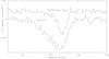 |
Fig. 9 Example absorption spectra of NH3(7, 7) and CH3OH(102,8−101,9) taken toward the northern cm continuum peak position. The CH3OH spectrum is shifted slightly to positive flux density values for better presentation. |
These observations clearly outline the complicated nature of studying high-mass accretion disks. On the one hand, extremely high spatial resolution at sub-0.1″ is required. However, that resolution is achievable now with observations at cm wavelength at the VLA, such as those presented here, or new observations with the Atacama Large Millimeter Array (ALMA) that can reach even higher resolution; however, this target NGC 7538IRS1 is too far north and not accessible with ALMA.
On the other hand, it is also crucial to identify the right sources and disk tracers. If we are dealing with hypercompact Hii regions, ionized tracers such as radio recombination lines could be very useful (e.g., Keto et al. 2008; Keto & Klaassen 2008; Klaassen et al. 2009). For NGC 7538IRS1, we did observe such recombination lines simultaneously, however, the sensitivity was insufficient for further analysis. Furthermore, as shown in Keto et al. (2008), where they present radio recombination line data toward NGC 7538IRS1 at 22 and 43 GHz, these lines at cm wavelengths are typically very broad. A significant amount of the line width at these wavelengths is caused by thermal and pressure broadening and disentangling kinematic signatures from these components is not trivial. Going to (sub)mm wavelengths may improve the situation because there at least the pressure broadening is significantly reduced. Therefore, it may be more promising to select sources at even earlier evolutionary phases where no hypercompact Hii region has formed yet; one hence can study the kinematics at much smaller scales in the molecular form.
5. Conclusions
Resolving the famous high-mass star-forming region NGC 7538IRS1 at the highest spatial resolution possible at cm wavelengths with the VLA (0.06″ × 0.05″ corresponding to ~150 AU) reveals several new insights into the physics of this archetypical high-mass star-forming region. Comparing the new data to previous epoch observations from ~23 yr ago, no proper motions can be identified. In combination with a high spectral index largely varying between 1 and 2, we infer that the cm continuum emission does not stem from an underlying jet, but that it is rather dominated by two hypercompact Hii regions that are likely formed by two separate high-mass protostars. Based on the kinematics, these protostars appear to form a bound system within a circumbinary envelope.
The CH3OH and NH3 spectral line data reveal different velocity structures in absorption against the strong continuum emission. The thermal CH3OH data show two velocity gradients across the two continuum sources, indicating the existence of two embedded disk-like structures. The approximate orientation and velocity structure of these thermal CH3OH measurements agree well with the much higher resolution CH3OH maser data (Moscadelli & Goddi 2014). While the two disk-like structures are almost parallel, the NH3 data trace a rotating circumbinary envelope that is inclined to the two disk-like structures by ~33°. Such variations in rotation axis between envelope- and disk-structures can be caused by varying initial angular momentum distribution in the natal, turbulent molecular cloud.
The fact that we do not identify Keplerian signatures in the disk-tracing CH3OH data is mostly caused by the nature of this molecular absorption line data, which do not trace the innermost gas that is ionized already. A closer investigation of the kinematics to the center will require recombination line observations, best conducted at (sub)mm wavelengths where the pressure broadening of the line becomes negligible.
Acknowledgments
We like to thank Luca Moscadelli and Ciriaco Goddi for providing the cm continuum data from 1992 and for giving the details about the positional uncertainties of the calibrator and the proper motions of the region. Furthermore, we thank Stella Offner for an interesting discussion about angular momentum vector distributions and their variations in turbulent cores. We would also like to thank the referee for a constructive and helpful report. This paper makes use of data from the Karl G. Jansky Very Large Array. The National Radio Astronomy Observatory is a facility of the National Science Foundation operated under cooperative agreement by Associated Universities, Inc. H.B. acknowledges support from the European Research Council under the Horizon 2020 Framework Program via the ERC Consolidator Grant CSF-648505.
References
- Arce, H. G., Shepherd, D., Gueth, F., et al. 2007, in Protostars and Planets V, eds. B. Reipurth, D. Jewitt, & K. Keil, 245 [Google Scholar]
- Beltrán, M. T., & de Wit, W. J. 2016, A&ARv, 24, 6 [NASA ADS] [CrossRef] [Google Scholar]
- Beltrán, M. T., Cesaroni, R., Neri, R., & Codella, C. 2011, A&A, 525, A151 [NASA ADS] [CrossRef] [EDP Sciences] [Google Scholar]
- Beuther, H., Schilke, P., Gueth, F., et al. 2002, A&A, 387, 931 [NASA ADS] [CrossRef] [EDP Sciences] [Google Scholar]
- Beuther, H., Churchwell, E. B., McKee, C. F., & Tan, J. C. 2007a, in Protostars and Planets V, eds. B. Reipurth, D. Jewitt, & K. Keil, 165 [Google Scholar]
- Beuther, H., Zhang, Q., Bergin, E. A., et al. 2007b, A&A, 468, 1045 [NASA ADS] [CrossRef] [EDP Sciences] [Google Scholar]
- Beuther, H., Walsh, A. J., & Longmore, S. N. 2009, ApJS, 184, 366 [NASA ADS] [CrossRef] [Google Scholar]
- Beuther, H., Linz, H., & Henning, T. 2012, A&A, 543, A88 [NASA ADS] [CrossRef] [EDP Sciences] [Google Scholar]
- Beuther, H., Linz, H., & Henning, T. 2013, A&A, 558, A81 [NASA ADS] [CrossRef] [EDP Sciences] [Google Scholar]
- Boley, P. A., Linz, H., van Boekel, R., et al. 2013, A&A, 558, A24 [NASA ADS] [CrossRef] [EDP Sciences] [Google Scholar]
- Boley, P. A., Kraus, S., de Wit, W.-J., et al. 2016, A&A, 586, A78 [NASA ADS] [CrossRef] [EDP Sciences] [Google Scholar]
- Bontemps, S., Motte, F., Csengeri, T., & Schneider, N. 2010, A&A, 524, A18 [NASA ADS] [CrossRef] [EDP Sciences] [Google Scholar]
- Brogan, C. L., Hunter, T. R., Cyganowski, C. J., et al. 2012, in Cosmic Masers – from OH to H0, eds. R. S. Booth, W. H. T. Vlemmings, & E. M. L. Humphreys, IAU Symp., 287, 497 [Google Scholar]
- Cesaroni, R., Neri, R., Olmi, L., et al. 2005, A&A, 434, 1039 [NASA ADS] [CrossRef] [EDP Sciences] [Google Scholar]
- Cesaroni, R., Galli, D., Lodato, G., Walmsley, C. M., & Zhang, Q. 2007, in Protostars and Planets V, eds. B. Reipurth, D. Jewitt, & K. Keil, 197 [Google Scholar]
- Chini, R., Hoffmeister, V. H., Nasseri, A., Stahl, O., & Zinnecker, H. 2012, MNRAS, 424, 1925 [NASA ADS] [CrossRef] [Google Scholar]
- Commerçon, B., Hennebelle, P., & Henning, T. 2011, ApJ, 742, L9 [NASA ADS] [CrossRef] [Google Scholar]
- Duarte-Cabral, A., Bontemps, S., Motte, F., et al. 2013, A&A, 558, A125 [NASA ADS] [CrossRef] [EDP Sciences] [Google Scholar]
- Franco, J., Kurtz, S., Hofner, P., et al. 2000, ApJ, 542, L143 [NASA ADS] [CrossRef] [Google Scholar]
- Frank, A., Ray, T. P., Cabrit, S., et al. 2014, in Protostars and Planets VI, eds. H. Beuther, R. S. Klessen, C. P. Dullemond, & T. Henning (Tucson: University of Arizona Press), 451 [Google Scholar]
- Gaume, R. A., Claussen, M. J., de Pree, C. G., Goss, W. M., & Mehringer, D. M. 1995a, ApJ, 449, 663 [NASA ADS] [CrossRef] [Google Scholar]
- Gaume, R. A., Goss, W. M., Dickel, H. R., Wilson, T. L., & Johnston, K. J. 1995b, ApJ, 438, 776 [NASA ADS] [CrossRef] [Google Scholar]
- Goddi, C., Zhang, Q., & Moscadelli, L. 2015, A&A, 573, A108 [NASA ADS] [CrossRef] [EDP Sciences] [Google Scholar]
- Guzmán, A. E., Garay, G., Rodríguez, L. F., et al. 2016, ApJ, 826, 208 [NASA ADS] [CrossRef] [Google Scholar]
- Henning, T., Schreyer, K., Launhardt, R., & Burkert, A. 2000, A&A, 353, 211 [NASA ADS] [Google Scholar]
- Ilee, J. D., Wheelwright, H. E., Oudmaijer, R. D., et al. 2013, MNRAS, 429, 2960 [NASA ADS] [CrossRef] [Google Scholar]
- Ilee, J. D., Cyganowski, C. J., Nazari, P., et al. 2016, MNRAS, 462, 4386 [NASA ADS] [CrossRef] [Google Scholar]
- Johnston, K. G., Robitaille, T. P., Beuther, H., et al. 2015, ApJ, 813, L19 [NASA ADS] [CrossRef] [Google Scholar]
- Keto, E. 2002, ApJ, 568, 754 [NASA ADS] [CrossRef] [Google Scholar]
- Keto, E. 2003, ApJ, 599, 1196 [NASA ADS] [CrossRef] [Google Scholar]
- Keto, E., & Klaassen, P. 2008, ApJ, 678, L109 [NASA ADS] [CrossRef] [Google Scholar]
- Keto, E., Zhang, Q., & Kurtz, S. 2008, ApJ, 672, 423 [NASA ADS] [CrossRef] [Google Scholar]
- Klaassen, P. D., Wilson, C. D., Keto, E. R., & Zhang, Q. 2009, ApJ, 703, 1308 [NASA ADS] [CrossRef] [Google Scholar]
- Klaassen, P. D., Galván-Madrid, R., Peters, T., Longmore, S. N., & Maercker, M. 2013, A&A, 556, A107 [NASA ADS] [CrossRef] [EDP Sciences] [Google Scholar]
- Knez, C., Lacy, J. H., Evans, II, N. J., van Dishoeck, E. F., & Richter, M. J. 2009, ApJ, 696, 471 [NASA ADS] [CrossRef] [Google Scholar]
- Kratter, K. M., & Matzner, C. D. 2006, MNRAS, 373, 1563 [NASA ADS] [CrossRef] [Google Scholar]
- Kraus, S., Hofmann, K., Menten, K. M., et al. 2010, Nature, 466, 339 [NASA ADS] [CrossRef] [MathSciNet] [PubMed] [Google Scholar]
- Kraus, S., Kluska, J., Kreplin, A., et al. 2017, ApJ, 835, L5 [NASA ADS] [CrossRef] [Google Scholar]
- Krumholz, M. R., Klein, R. I., & McKee, C. F. 2007, ApJ, 665, 478 [NASA ADS] [CrossRef] [Google Scholar]
- Krumholz, M. R., Klein, R. I., McKee, C. F., Offner, S. S. R., & Cunningham, A. J. 2009, Science, 323, 754 [NASA ADS] [CrossRef] [PubMed] [Google Scholar]
- Kuiper, R., & Yorke, H. W. 2013, ApJ, 772, 61 [NASA ADS] [CrossRef] [Google Scholar]
- Kuiper, R., Klahr, H., Beuther, H., & Henning, T. 2010, ApJ, 722, 1556 [CrossRef] [Google Scholar]
- Kuiper, R., Klahr, H., Beuther, H., & Henning, T. 2011, ApJ, 732, 20 [NASA ADS] [CrossRef] [Google Scholar]
- Leurini, S., Menten, K. M., & Walmsley, C. M. 2016, A&A, 592, A31 [NASA ADS] [CrossRef] [EDP Sciences] [Google Scholar]
- López-Sepulcre, A., Codella, C., Cesaroni, R., Marcelino, N., & Walmsley, C. M. 2009, A&A, 499, 811 [NASA ADS] [CrossRef] [EDP Sciences] [Google Scholar]
- Lovas, F. 2004, J. Phys. Ref. Data, 33, 177 [Google Scholar]
- Martí, J., Rodríguez, L. F., & Reipurth, B. 1998, ApJ, 502, 337 [NASA ADS] [CrossRef] [Google Scholar]
- Menten, K. M., Walmsley, C. M., Henkel, C., & Wilson, T. L. 1986, A&A, 157, 318 [NASA ADS] [Google Scholar]
- Moscadelli, L., & Goddi, C. 2014, A&A, 566, A150 [NASA ADS] [CrossRef] [EDP Sciences] [Google Scholar]
- Moscadelli, L., Reid, M. J., Menten, K. M., et al. 2009, ApJ, 693, 406 [NASA ADS] [CrossRef] [Google Scholar]
- Müller, H. S. P., Thorwirth, S., Roth, D. A., & Winnewisser, G. 2001, A&A, 370, L49 [NASA ADS] [CrossRef] [EDP Sciences] [Google Scholar]
- Palau, A., Fuente, A., Girart, J. M., et al. 2013, ApJ, 762, 120 [NASA ADS] [CrossRef] [Google Scholar]
- Peter, D., Feldt, M., Henning, T., & Hormuth, F. 2012, A&A, 538, A74 [NASA ADS] [CrossRef] [EDP Sciences] [Google Scholar]
- Peters, T., Klessen, R. S., Mac Low, M.-M., & Banerjee, R. 2010, ApJ, 725, 134 [NASA ADS] [CrossRef] [Google Scholar]
- Purser, S. J. D., Lumsden, S. L., Hoare, M. G., et al. 2016, MNRAS, 460, 1039 [NASA ADS] [CrossRef] [Google Scholar]
- Reynolds, S. P. 1986, ApJ, 304, 713 [NASA ADS] [CrossRef] [Google Scholar]
- Rodón, J. A., Beuther, H., & Schilke, P. 2012, A&A, 545, A51 [NASA ADS] [CrossRef] [EDP Sciences] [Google Scholar]
- Sana, H., de Mink, S. E., de Koter, A., et al. 2012, Science, 337, 444 [Google Scholar]
- Sánchez-Monge, Á., Cesaroni, R., Beltrán, M. T., et al. 2013, A&A, 552, L10 [NASA ADS] [CrossRef] [EDP Sciences] [Google Scholar]
- Sánchez-Monge, Á., Beltrán, M. T., Cesaroni, R., et al. 2014, A&A, 569, A11 [NASA ADS] [CrossRef] [EDP Sciences] [Google Scholar]
- Sandell, G., Goss, W. M., Wright, M., & Corder, S. 2009, ApJ, 699, L31 [NASA ADS] [CrossRef] [Google Scholar]
- Schöier, F. L., van der Tak, F. F. S., van Dishoeck, E. F., & Black, J. H. 2005, A&A, 432, 369 [NASA ADS] [CrossRef] [EDP Sciences] [Google Scholar]
- Sobolev, A. M., & Strelnitskii, V. S. 1983, Sov. Astron. Lett., 9, 12 [NASA ADS] [Google Scholar]
- Sobolev, A. M., Wallin, B. K., & Watson, W. D. 1998, ApJ, 498, 763 [NASA ADS] [CrossRef] [Google Scholar]
- Stahler, S. W., & Palla, F. 2005, The Formation of Stars (Wiley-VCH) [Google Scholar]
- Tan, J. C., Beltrán, M. T., Caselli, P., et al. 2014, in Protostars and Planets VI (Tucson: University of Arizona Press), 149 [Google Scholar]
- Vaidya, B., Fendt, C., & Beuther, H. 2009, ApJ, 702, 567 [NASA ADS] [CrossRef] [Google Scholar]
- Voronkov, M. A., Brooks, K. J., Sobolev, A. M., et al. 2007, in Astrophysical Masers and their Environments, eds. J. M. Chapman, & W. A. Baan, IAU Symp., 242, 182 [Google Scholar]
- Wang, K., Zhang, Q., Wu, Y., & Zhang, H. 2011, ApJ, 735, 64 [NASA ADS] [CrossRef] [Google Scholar]
- Willner, S. P. 1976, ApJ, 206, 728 [NASA ADS] [CrossRef] [Google Scholar]
- Yorke, H. W., & Sonnhalter, C. 2002, ApJ, 569, 846 [NASA ADS] [CrossRef] [Google Scholar]
- Zhang, Q., Hunter, T. R., Brand, J., et al. 2005, ApJ, 625, 864 [NASA ADS] [CrossRef] [Google Scholar]
- Zhang, Q., Wang, Y., Pillai, T., & Rathborne, J. 2009, ApJ, 696, 268 [NASA ADS] [CrossRef] [Google Scholar]
- Zhu, L., Zhao, J.-H., Wright, M. C. H., et al. 2013, ApJ, 779, 51 [NASA ADS] [CrossRef] [Google Scholar]
- Zinnecker, H., & Yorke, H. W. 2007, ARA&A, 45, 481 [NASA ADS] [CrossRef] [Google Scholar]
All Tables
All Figures
|
Fig. 1 Centimeter continuum emission from NGC 7538IRS1. The left panel shows in color scale the new 1.2 cm continuum data imaged using only baselines between 10 and 37 km, achieving a spatial resolution of 0.06″ × 0.05″. The contours present for comparison the old VLA data from 1992 discussed previously in Gaume et al. (1995a), Sandell et al. (2009), Moscadelli & Goddi (2014), and Goddi et al. (2015) starting at the 4σ contour and continuing in 8σ intervals (1σ ~ 0.05 mJy beam-1). The two stars indicate the CH3OH maser positions by Moscadelli & Goddi (2014); see Sect. 3.1 for more details. The middle panel shows in color the spectral index map derived from the new full dataset with robust weighting −2 and the contours show the corresponding continuum image using all data at a resolution of 0.07″ × 0.05″. The contour levels start at a 4σ levels of 0.16 mJy beam-1 and continue in coarser 32σ steps. The right panel again shows the new 0.06″ × 0.05″ data, now converted in the Rayleigh-Jeans approximation to brightness temperature. |
| In the text | |
|
Fig. 2 NH3 example spectra extracted toward the northern cm continuum peak position. The spectra are shifted of the y-axis for presentation purposes. All lines are labeled. |
| In the text | |
|
Fig. 3 CH3OH example spectra extracted toward the northern cm continuum peak position. The spectra are shifted of the y-axis for presentation purposes. All lines are labeled. |
| In the text | |
|
Fig. 4 Color-scale presents the 1st moment maps (intensity-weighted velocities) of the NH3 inversion transitions from (1, 1) to (7, 7) as indicated in each panel. The first two left panels show the data for the NH3(1, 1) line with different weighting schemes (natural weighting and robust weighting, which is a hybrid between natural and uniform weighting). The other NH3 lines are always presented with robust weighting 0. The 1st moment maps are clipped at a ~4σ level. The contours show in all panels the 1.2 cm continuum emission in levels of 8% to 98% of the peak emission (7.4 mJy beam-1). The two stars indicate the CH3OH maser positions by Moscadelli & Goddi (2014). The line in the bottom right panel indicates the position-velocity cut shown below. |
| In the text | |
|
Fig. 5 Position-velocity diagrams for the different NH3 inversion lines as indicated in each panel. The direction of the cut is shown in Fig. 4. The top left and top 2nd panels show this cut for natural and robust weighting for the NH3(1, 1) lines, respectively. All other cuts are carried out for the robust weighting case. |
| In the text | |
|
Fig. 6 Integrated (left) and 2nd moment (right) maps (intensity-weighted velocity dispersion) for two NH3 and one CH3OH line as indicated in each panel. The integration ranges for NH3(3, 3), (7, 7) and CH3OH(102,8−101,9) are [–68, –50] km s-1, [–65, –50] km s-1 and [–65, –53] km s-1, respectively. The contours show in all panels the 1.2 cm continuum emission in levels of 8% to 98% of the peak emission (7.4 mJy beam-1). The two stars indicate the CH3OH maser positions by Moscadelli & Goddi (2014). The synthesized beams are shown in the bottom left of each panel. |
| In the text | |
|
Fig. 7 Color-scale presents the 1st moment maps (intensity-weighted velocities) of the CH3OH lines as shown in each panel. The contours show in all panels the 1.2 cm continuum emission in levels of 8% to 98% of the peak emission (7.4 mJy beam-1). The two stars indicate the CH3OH maser positions by Moscadelli & Goddi (2014). The two lines in the bottom right panel indicate the cuts for the position-velocity diagrams shown below. |
| In the text | |
|
Fig. 8 Position-velocity diagrams for the different CH3OH lines as indicated in each panel. The top seven panels belong to the northern cut and the bottom seven panels to the southern cut shown in Fig. 7. All cuts are performed for the robust weighting 0 case. |
| In the text | |
|
Fig. 9 Example absorption spectra of NH3(7, 7) and CH3OH(102,8−101,9) taken toward the northern cm continuum peak position. The CH3OH spectrum is shifted slightly to positive flux density values for better presentation. |
| In the text | |
Current usage metrics show cumulative count of Article Views (full-text article views including HTML views, PDF and ePub downloads, according to the available data) and Abstracts Views on Vision4Press platform.
Data correspond to usage on the plateform after 2015. The current usage metrics is available 48-96 hours after online publication and is updated daily on week days.
Initial download of the metrics may take a while.