| Issue |
A&A
Volume 605, September 2017
|
|
|---|---|---|
| Article Number | A76 | |
| Number of page(s) | 26 | |
| Section | Catalogs and data | |
| DOI | https://doi.org/10.1051/0004-6361/201629936 | |
| Published online | 14 September 2017 | |
A spectroscopic survey of Orion KL between 41.5 and 50 GHz⋆
1 Departamento de Astrofísica, Centro de Astrobiología (INTA-CSIC), Ctra. M-108, km 4, 28850 Torrejón de Ardoz, Spain
e-mail: ricardo.rizzo@cab.inta-csic.es
2 Grupo de Astrofísica Molecular, Instituto de Ciencia de Materiales de Madrid (CSIC), Calle Sor Juana Inés de la Cruz 3, Cantoblanco, 28049 Madrid, Spain
Received: 21 October 2016
Accepted: 20 May 2017
Context. The nearby massive star-forming region Orion KL is one of the richest molecular reservoirs known in our Galaxy. The region hosts newly formed protostars, and the strong interaction between their radiation and their outflows with the environment results in a series of complex chemical processes leading to a high diversity of interstellar tracers. The region is therefore one of the most frequently observed sources, and the site where many molecular species have been discovered for the first time.
Aims. Current availability of wideband backends permits us to efficiently perform spectral surveys in the entire mm-range. We aim to study the almost unexplored 7 mm window in Orion KL to obtain an unbiased chemical picture of the region.
Methods. In this paper we present a sensitive spectral survey of Orion KL, made with one of the 34 m antennas of the Madrid Deep Space Communications Complex in Robledo de Chavela, Spain. The spectral range surveyed is from 41.5 to 50 GHz, with a frequency spacing of 180 kHz (equivalent to ≈1.2 km s-1, depending on the exact frequency). The rms achieved ranges from 8 to 12 mK.
Results. The spectrum is dominated by the J = 1 → 0 SiO maser lines and by radio recombination lines (RRLs), which were detected up to Δn = 11. Above a 3σ level, we identified 66 RRLs and 161 molecular lines corresponding to 39 isotopologues from 20 molecules; a total of 18 lines remain unidentified, two of them above a 5σ level. Results of radiative modelling of the detected molecular lines (excluding masers) are presented.
Conclusions. At this frequency range, this is the most sensitive survey and also the one with the largest bandwidth. Although some complex molecules like CH3CH2CN and CH2CHCN arise from the hot core, most of the detected molecules originate from the low temperature components in Orion KL.
Key words: line: formation / surveys / stars: formation / ISM: clouds / ISM: molecules / radio lines: ISM
The reduced spectrum is only available at the CDS via anonymous ftp to cdsarc.u-strasbg.fr (130.79.128.5) or via http://cdsarc.u-strasbg.fr/viz-bin/qcat?J/A+A/605/A76
© ESO, 2017
1. Introduction
Orion KL has been widely recognized as the nearest high-mass star-forming region at a distance of 414–418 pc (Menten et al. 2007; Kim et al. 2008), and one of the richest molecular reservoirs known in the Galaxy.
It hosts newly formed protostars, with strong interaction between their radiation and their outflows with the environment. Diverse chemical processes are therefore favoured in the region, which results in a high variety of molecules detected. Indeed, this is the site at which many molecular species have been discovered for the first time (e.g. methyl acetate, Tercero et al. 2013). After several observational works (e.g. Blake et al. 1987; Schilke et al. 2001; Tercero et al. 2010; Gong et al. 2015), at least four different molecular components have been identified in a relatively small volume. There are two compact sources, the hot core, characterized by high temperatures (TK ~100−300 K) and the compact ridge, with TK ~100−150 K. The third component is a quite extended plateau (with an angular size of up to 30′′), characterized by a warm molecular outflow at TK ~150 K). The hot core, the compact ridge and the outflow are immersed within the cooler (TK ~40−60 K) extended ridge or ambient cloud. These gas components could be resolved with single dish telescopes because they display different radial velocities and line widths. The Orion KL region is therefore an excellent testbed for the search of new molecules and also for the chemical characterization of those already known.
Many spectral line surveys have been carried out towards Orion KL covering a large range of frequencies (see Table 1 of Gong et al. 2015). In recent years, there have been the IRAM 30 m millimeter survey (Tercero et al. 2010), the Herschel/ HIFI submillimeter and Far IR survey (Crockett et al. 2014), the submillimeter survey carried out with the Odin satellite (Olofsson et al. 2007; Persson et al. 2007), and the Effelsberg-100 m telescope 1.3 cm survey (Gong et al. 2015).
However, the spectral range around 7 mm remains almost unexplored. To the best of our knowledge, the most complete survey up to date is that of Goddi et al. (2009a), which covers a frequency range optimized for the J = 1 → 0 SiO maser emission lines (from 42.3 to 43.6 GHz).
Besides the SiO lines, the 40–50 GHz spectral window is potentially rich in several complex organic molecules, and hosts several transitions also identified at higher frequencies (3, 2, and 1 mm), but at lower energy levels. At these frequencies the presence of a wealth of radio recombination lines (RRLs) is also remarkable.
In this paper we present the results of a spectral survey in the Orion KL region, in the frequency range from 41.5 to 50 GHz (6 to 7.2 mm in wavelength). Section 2 describes the technical aspects of the survey, while Sect. 3 summarizes the results. A radiative model of the molecular emission is presented in Sect. 4, and the conclusions are enumerated in Sect. 5.
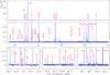 |
Fig. 1 Spectrum of Orion KL. Top panel: full range. Middle panel: magnification in intensity to see low intensity lines; green boxes are expanded in the three bottom panels, to show spectroscopic details. Some of the most intense lines are labelled. |
2. The spectral survey
We used the DSS-54 antenna, one of the 34 m dishes available at the NASA’s Madrid Deep Space Communications Complex (MDSCC), to perform a sensitive spectral survey of Orion KL. The observations were done in different runs from December 2013 to February 2014.
The survey was performed using a cooled high electron mobility transistor (HEMT) receiver (Rizzo & García-Miró 2013) and the two circular polarizations have been recorded. The receiver temperature remained around 40 K. The resulting system temperature varied from 90 to 190 K (in antenna temperature units), depending on the frequency, elevation and weather conditions. The backend was a new wideband backend (Rizzo et al. 2012), which provides 1.5 GHz of instantaneous bandwidth and a resolution of 180 kHz (equivalent to ≈1.2 km s-1 at the observed frequencies), for each circular polarization.
The survey was conducted in position switching mode in six sub-bands, with a superposition of 100 MHz between two consecutive sub-bands, in order to check consistency and eliminate possible image sideband effects. Total integration time was 1490 min (on source). For each sub-band the integration time varied from 97 to 422 min, in order to reach to a uniform rms (1σ) level between 4 and 6 mK, on an antenna temperature scale.
Observations were carried out in winter nights, under good weather conditions. The atmospheric opacity was measured during each observing session by means of tipping curves, and was between 0.07 and 0.11. During the observations, individual spectra have been corrected by atmospheric opacity and antenna gain due to elevation, obtaining the antenna corrected scale ( ).
).
Data were processed using CLASS, a part of the GILDAS software1. Spectra from different runs were averaged and baseline subtracted. The final spectrum was converted to main beam brightness temperature (Tmb) according to the usual expression  (1)where ηmb is the main beam efficiency (Wilson et al. 2009). The most relevant antenna parameters for different scale conversions, including density flux S, are summarized in Table 1. Unless otherwise specified, we use the Tmb scale throughout the paper.
DSS-54 antenna parameters.
3. Results
3.1. Overall emission
Figure 1 shows the resulting spectrum in the whole observed band. The upper panel displays the full range both in frequency and in intensity. We see that the spectrum is dominated by the emission of SiO masers and RRLs. Some well known molecules (CS, H2CO, HC3N, CH3OH) are also intense and usually associated with both, cold and hot gas.
The middle panel depicts a zoom in intensity, where it is possible to distinguish a number of other, more complex molecules, particularly SO2, CH3CH2CN, HNCO, CH3OCOH, and OCS. As shown in the model (Sect. 4), these molecules are associated with the hottest parts of the region.
The three lower panels are small spectral windows (indicated in green in the middle panel) which display the richness of spectral lines and different line widths. We identified a total of 66 RRLs and 161 molecular lines above a 3σ level, of which 18 lines remain unidentified (U lines hereafter). The relative number of molecular lines with respect to RRLs is therefore 161/66 ≈ 2.4. This is approximately four times higher than the ratio obtained at 1.3 cm (for example Gong et al. 2015, who detected 164 RRLs and 97 molecular lines), but notably lower than that found at millimeter wavelengths, where Tercero et al. (2010) identified more than 14 400 molecular lines but only a few dozens of RRLs.
Therefore, the 7 mm band is especially useful in carrying out spectroscopic studies where the emission of RRLs and molecular lines are both of interest. Within some GHz of bandwidth, this band has a well balanced number of RRLs and molecular lines. At cm wavelengths, the number of molecular lines is quite low, while at mm wavelengths the high density of molecular lines and the large separation in frequency of the RRLs makes it difficult to simultaneously study the atomic ionized and the molecular components.
The procedure employed for line identification (such as smoothing, catalogues, and cross-check with other surveys) is outlined in Sect. 4.
3.2. Radio recombination lines
The detected 66 RRLs include 50, 12, and 4 lines corresponding to hydrogen, helium, and carbon, respectively. Hydrogen has been detected at a maximum Δn (the difference between principal quantum numbers of the upper and lower levels) of 11. All the detected lines can be well characterized by Gaussian fittings, whose parameters are indicated in Table A.1. For each detection, the table contains the line name (ordered by increasing Δn), frequency, velocity-integrated line intensity, peak velocity, full width at half maximum, and peak temperature. One-sigma errors are displayed within parenthesis. Frequencies have been obtained from the MADCUBA_IJ package2.
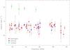 |
Fig. 2 Distribution of the velocities of the RRLs as a function of frequency. Atoms (hydrogen, helium, and carbon) are labelled in red, blue, and green, respectively. |
Possible blending with molecular lines or other RRLs are indicated as notes in the last column of Table A.1. In some cases (H64β, H83δ, and H107κ) we could not separate the contribution of the blending lines, and the corresponding fitting has not been considered in subsequent analysis. The line H81δ is clearly detected, but the spectrum is suffering from a series of unwanted features in specific channels (“spikes”) at close frequencies; therefore, the fitting seriously underestimates the line intensity (probably up to a factor of three).
For each atom, Fig. 2 depicts the distribution of velocities as a function of frequencies. The unweighted mean velocities of hydrogen and helium agree within uncertainties, with values of −4.0 ± 1.2 km s-1 for hydrogen and −3.6 ± 1.8 km s-1 for helium, while for the carbon lines we obtain + 9.3 ± 1.9 km s-1. To compute these values we included all the lines detected not affected by blending, and the error was estimated as the maximal individual error divided by the square root of the number of lines. The corresponding mean velocities weighted by the inverse square of the individual errors are −2.9 ± 0.1, −3.0 ± 0.4, and + 9.4 ± 0.7 km s-1 for hydrogen, helium and carbon, respectively. As expected, these values are dominated by the α lines which have the smallest uncertainties. The computed velocities are compatible with hydrogen and helium arising from the Hii region M42, while the carbon recombination lines originate from the photon-dominated region (PDR) at the interface between M42 and the associated molecular cloud (the Orion Bar, see Cuadrado et al. 2015; Gong et al. 2015).
Based on their own data and other works, Goddi et al. (2009a) reported that RRL velocities increase with frequency, and explain this effect by the presence of a density gradient within the Hii region. We decided to explore such hypothesis with a careful literature search. First, Goddi et al. (2009a) report “velocities ranging from −5 to −10 km s-1” based on three RRLs (H53α, He53α, and H76γ), but they do not provide individual fitting; we measure a mean velocity of the H53α line of −3.29 ± 0.04 km s-1. Second, the other observations used for the hypothesis are those at 71−122 GHz from Turner (1991; 18 RRLs, including four α lines from hydrogen) and at 215−247 GHz from Sutton et al. (1985; 2 RRLs, only one α line from hydrogen). Turner (1991) reported a mean velocity of −3.4 km s-1, but unfortunately did not provide individual fitting of the lines. Sutton et al. (1985) reported +4 km s-1 for the H30α line, but this is clearly contaminated by a rather strong line of 33SO2 at ≈231.9003 GHz (Esplugues et al. 2013a).
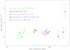 |
Fig. 3 LSR velocities of α RRLs from hydrogen in Orion KL, as a function of the frequency (on a logarithmic scale). Surveys used are indicated with different colours. Together with the references, the principal quantum numbers are indicated within parenthesis. Error bars correspond to 2σ values. |
Since the work of Goddi et al. (2009a), several new surveys have been performed at different wavelengths. We therefore searched for the available information about α RRLs from hydrogen. Besides our own survey, we selected those works providing individual fitting (Sutton et al. 1985; Gong et al. 2015), or with the possibility of gathering frequency calibrated data, as the IRAM 30 m data provided by Tercero et al. (2010) and the GBT 4 mm survey of Frayer et al. (2015), available online3. The results are summarized in Table A.2, and depicted in Fig. 3. Data include Gaussian fitting of α hydrogen RRL velocities from H30α to H71α, covering a wide range of frequencies from 17 to 232 GHz. In neither the figure or the table do we see any significant variation of the velocities at any frequency, except the H30α line, which is affected by blending, as already commented above. Therefore, we have not found any evidence for the claimed density gradient in the Hii region.
Line widths are also quite uniform for each atom. We computed mean values of 21.9 ± 3.4, 16.4 ± 6.2, and 5.4 ± 3.4 km s-1 for hydrogen, helium and carbon, respectively, which are in agreement with previous results (Gong et al. 2015).
In order to test the physical conditions of the Hii region, we computed the ratio of peak temperatures for two hydrogen RRLs which lie at close frequencies. These ratios were then compared to the expected values under LTE conditions, following the procedure outlined by Brocklehurst & Seaton (1972). We excluded the ratios involving the H81δ and H83δ lines (see notes in Table A.1). The result is depicted in Fig. 4, where the measured ratios are plotted as a function of the LTE ratio. In this figure we see that the excitation of RRLs at these frequencies are close to LTE, within the uncertainties.
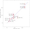 |
Fig. 4 Distribution of the measured line intensity ratios between pairs of hydrogen RRLs at nearby frequencies as a function of the predicted ratios under LTE conditions. The ratios are labelled and the bars represent 1.5σ errors. The dotted blue line corresponds to equal values between observed and predicted ratios under LTE conditions. |
We also measured the helium abundance by computing the velocity-integrated line ratio between the same RRL from helium and hydrogen. We used all the available α, β, and γ lines, excluding H64β due to blending. These ratios are a measure of the helium abundance under LTE conditions, assuming that all the helium is singly ionized and both Strömgren spheres are identical. The resulting value is 8.3 ± 1.2%, which agrees with previous measurements in this source (Gong et al. 2015), and is close to Solar System values (Wilson & Rood 1994).
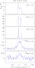 |
Fig. 5 The SiO J = 1 → 0 lines detected in Orion KL. Isotopologues and vibrational numbers are indicated in each panel. |
3.3. SiO emission
We detected a total of five lines from SiO, which are shown in Fig. 5. The lines correspond to the vibrational numbers v = 0, 1, and 2 of the main isotopologue, and to v = 0 of 29SiO and 30SiO. Overall, the line shapes agree with the single-dish results presented by Goddi et al. (2009a).
The most intense lines are masers corresponding to v = 1 and 2 of the main isotopologue. These lines are double-peaked and cover the velocity range from −16 to +27 km s-1. Goddi et al. (2009b) have mapped these lines using the Very Large Array (VLA) and found that the emission arises from the inner part of the circumstellar structure associated with Source I, with a maximum size of 100 AU.
The bright and very narrow feature in the v = 2 line at ≈−1.4 km s-1 is reported here for the first time. This component is not present in previous observations of Goddi et al. (2009a,b), obtained with even better spectral resolution. The lack of a similar feature in the v = 1 line may indicate that the emission of both maser lines arises from slightly different regions, as Goddi et al. (2009b) suggested.
The bulk of the v = 0 emission from 29SiO and 30SiO lines appears as a single component matching approximately the same velocity range as the v = 1 and 2 lines of 28SiO. The high resolution maps (Goddi et al. 2009b) show that the emission of the four lines is confined to a distance of ≈100 AU to a young stellar object known as Source I. Goddi et al. (2009b) also pointed out significant variations (at least two orders of magnitude) in the brightness temperature. The above facts and further modelling of radiative pumping allow the authors to conclude that the 29SiO and 30SiO v = 0 line emission is non thermal.
The line shape of the v = 0 line from 28SiO is similar to those of 29SiO and 30SiO, although it has a broader spatial distribution (Goddi et al. 2009b), probably due to an outflow or a disc with a size of ≈600 AU in size, produced in the last 103 yr (Tercero et al. 2011; Niederhofer et al. 2012).
The emission of the ground vibrational state of 28SiO has been observed at several rotational transitions up to J = 8 → 7 (e.g. Beuther et al. 2005; Tercero et al. 2011; Niederhofer et al. 2012). All these lines except J = 1 → 0 have Gaussian-like shapes and do not show hints of maser emission (in fact, Tercero et al. 2011, satisfactorily modelled their emission under thermal regimes). The shape of the v = 0, J = 1 → 0 spectrum, as shown here, is rather different from the other v = 0 lines of 28SiO and the thermal modelling of Tercero et al. (2011) is not able to reproduce the observed shape and intensity. Therefore it seems probable that the line is caused at least partially by maser emission, which has also been proposed by Chandler & de Pree (1995).
In addition to the main velocity component, the v = 0 lines of the three isopotologues have large wings from −40 to +60 km s-1. The wings have been mapped in other rotational lines using interferometers: (J = 1 → 0: Goddi et al. 2009b, VLA), (J = 2 → 1: Plambeck et al. 2009, CARMA), and (J = 5 → 4, 6 → 5: Zapata et al. 2012; Niederhofer et al. 2012, ALMA). All those high resolution observations show that this wide component arises from a bipolar outflow driven by Source I (Goddi et al. 2009b).
Line list.
4. Radiative model of the molecular emission
4.1. Overall description
Figure A.1 displays the observed spectrum with more detail, after applying Hanning-smoothing of four contiguous channels, that is after degrading the spectral resolution to ~0.7 MHz. The intensity scale was in some cases magnified to improve the visibility of weak lines. Superimposed on the observed spectrum is also the result of the line identification and further modelling. The SiO species and RRLs, although identified, are not part of the model.
The complete list of the identified species is presented in Table 2. The frequencies have been obtained from the CDMS4 (Müller et al. 2001, 2005), the JPL5 (Pickett et al. 1998), and private catalogues (J. Cernicharo, priv. comm.). In all cases, we selected the frequency having the highest precision or that which provides the most complete information about hyperfine components. Most of the lines have been successfully identified, with only two U lines at a 5−6σ level, at 46 387.9 and 49 765.7 GHz. The first U line has a width of ≈10 km s-1, while the second one has ≈20 km s-1. If confirmed, the 46 387.9 GHz line may arise from the hot core and the other one from the plateau. Due to the low signal-to-noise ratio, it is difficult to provide a robust characterization of the line shapes. All lines identified in this survey correspond to abundant molecules previously detected in this source (e.g. Blake et al. 1987; Sutton et al. 1995; Schilke et al. 2001; Goddi et al. 2009a; Tercero et al. 2010, 2011).
For many of the identified species, we previously derived physical parameters and column densities based on data from the IRAM line survey at 3, 2 and 1.3 mm (Tercero et al. 2010), which have been already published in a series of papers (see Table B3 of Cernicharo et al. 2016, for references). Due to the wide frequency range of that survey and the detailed analysis of the different components, we expect that the previous results for the modelled species are well constrained. Therefore, as a first approach we applied the models already performed to fit the lines of the IRAM 30 m line survey to model the molecular emission at 7 mm.
We have built new radiative models for those molecules lacking previous modelling at this or other frequency bands after considering the differences attained from the use of different telescopes and frequencies. We fitted simultaneously both the cold and hot components in all the species. To do so, we used the MADEX code (Cernicharo 2012), which solves simultaneously the radiative transfer and the statistical equilibrium equations using local thermodynamic equilibrium (LTE); when the collisional rates were available, we proceeded with the large velocity gradient approach (LVG). A total of 5020 species from 1107 families6 can be modelled by this code.
We introduced the physical parameters of the different components found in the source (kinetic temperature TK, H2 volume density n(H2), source diameter dsou, LSR velocity vLSR, and line width Δv) according to either the typical values found in the literature and our previous Gaussian analysis of the lines. Furthermore, we also have taken into account the telescope dilution and the relative offsets between each cloud component with respect to the pointing position. We have chosen the column density of each cloud component as the free parameter. This method is iterative, which allowed us to introduce corrections to the original values of TK and n(H2) in LVG calculations to improve the fitting. The discrepancies between the original and corrected values were below 20% in all cases.
At some frequencies, baseline fluctuations may produce differences in line intensity up to ΔTmb ~ ± 0.02 K. Therefore, the uncertainties may grow up to 20% for those lines having an observed intensity below Tmb = 0.05 K
We estimated the uncertainties of the resulting column densities supported by the analysis already done in the IRAM 30 m survey (Tercero et al. 2010). There is not a remarkable new source of uncertainties in the new data presented in this work, especially for the molecules displaying a high signal-to-noise ratio in their lines. According to this analysis, the newly modelled molecules have uncertainties in the column density below 30%.
The physical parameters and the column densities obtained by the models are summarized in Table A.3, where the contribution of every molecule to the different components is presented. Detailed results for each species are discussed in the next two subsections.
4.2. Agreement with models for the IRAM 30 m survey
Most of the molecules with previous models have the bulk of their emission arising from the hot core. As described in the previous section, we used the physical parameters of those models as initial guesses.
We satisfactorily reproduced the emission of some of these species (HCS+, CCS, NH2CHO, CH3CH2CN ν13/ν21, 34SO2, 33SO2, HC3N ν6 = 1, and CH2CHCN) without having to modify any parameters in the models (Tercero et al. 2010; Motiyenko et al. 2012; Daly et al. 2013; Esplugues et al. 2013a,b; López et al. 2014). Table A.3 shows that these molecules have minor or absent contributions from the extended ridge and are therefore well described by the models at 1, 2, and 3 mm. In the case of NH2CHO, the upper limit to the column density in this survey is well constrained by the model of Motiyenko et al. (2012).
Some other species (CH3CH2CN, SO2, 13CH3OH, HC3N, HC5N, OCS, CS, C3S, and HNCO) are more ubiquitous and have significant contribution from both the hot and the cold components. We have adapted the models of Daly et al. (2013) for CH3CH2CN, Esplugues et al. (2013a) for SO2, Kolesniková et al. (2014) for 13CH3OH, Esplugues et al. (2013b) for HC3N and HC5N, Tercero et al. (2010) for OCS, CS, and C3S, and Marcelino et al. (2009) for HNCO in order to properly fit the lines of these species. In all cases, it was necessary to modify the column densities of the cold components with respect to the previous models. For SO2, CH3CH2CN and 13CH3OH we had to reduce the column densities of the extended ridge by a factor of two.
The case of 13CS is the most outstanding, whose column dentisty has been reduced by up to a factor of ten in the cold component. This drastic change implies an intriguingly high N(CS)/N(13CS) ratio (from 100 to 250), which should be studied through future and more detailed observations and models. For C3S we introduced for the first time an extended ridge component, which is evident in the J = 8 → 7 line (with upper level energy around 10 K).
In the case of C33S we detected only a narrow line, compatible with the extended ridge, which is by far the major contributor to the line profile. The warm components remain at an intensity level below 0.05 K, corresponding to the upper limits quoted in Table A.3.
In short, we noted that the 7 mm lines are more sensitive to small variations in the column densities of the cold component than lines at shorter wavelengths. This survey is, therefore, more adequate to constrain the contribution of the extended ridge gas.
Although all species discussed here have been previously detected in this source, some of them are only tentatively identified near the detection limit of our data: NH2CHO, O13CS, CCS, 33SO2, CH3CH2CN ν13/ν21, and HC3N ν7 = 2 (see Fig. A.1). Therefore, the derived column densities for these species have to be considered as upper limits.
4.3. New models
CH3OH (methanol). A total of ten lines of the main isotopologue of methanol are detected, equally distributed in A- and E- substates. Six of the lines are in the ground vibrational state, and four of them correspond to the first vibrationally excited state. The only maser is the 70 → 61A+ transition, which is a well known class I maser in several Galactic sources, including Orion KL (e.g. Haschick et al. 1990). Orion KL was, in fact, the first source where a methanol maser line was detected (Barrett et al. 1971). The 70 → 61A+ line shape (Haschick et al. 1990) is remarkably similar to the 80 → 71A+ line (Ohishi et al. 1986), having a thermal component of ≈4 km s-1 and a very narrow maser component with a width of only 0.22 km s-1 or less. Unfortunately, the spectral resolution of this survey prevents us to separate both components. Models of methanol in both the ground state and in its first vibrationally excited state have been performed considering the same components as those used for 13CH3OH. We note that the abundance ratio [CH3OH]/[13CH3OH] is between 5−15 for the different components. These values are far from the isotopic 12C/13C ratio of 45 derived by Tercero et al. (2010) in the source. Therefore, the lines from the main isotopologue of this abundant organic species are optically thick also at these frequencies. The derived column density for the hottest component (300 K) of A-CH3OH νt = 1 is a factor 10 higher than that of the E-substate. Only one line of A-CH3OH νt = 1 with Eu = 426 K appears in this survey above the detection limit whereas the energies of the lines of the E-species are around ~300 K (see Table 2). Due to this difference in energy we obtain a different value for the column densities in the A- and E-substates. The low number of lines prevents a detailed analysis and we cannot accurately constrain the column densities.
H2CO (formaldehyde). Ortho and para formaldehyde have been modelled for all the lines between 7 mm and 1 mm. The ortho-to-para ratio is approximately three, as expected at high gas temperature. Only one line of o-H213CO with low intensity (Sij< 0.5) is expected in the present frequency range, at 45.9 GHz. Because this line is only tentatively detected, the o-H213CO column density has to be considered as an upper limit.
CH3OCOH (methyl formate). Ground state and vibrationally excited species (νt = 0,1) have been identified in the present data. For the model, we used the same components provided by Margulès et al. (2010). Lines corresponding to b-type transitions arising in the IRAM 30 m data and the lines of the present survey have been fitted simultaneously. It is worth noting that the difference in the a and b dipole moments (μa = 1.63 and μb = 0.68 from Curl 1959) affects the opacity of the lines: many of the a-type transition-lines arising in the IRAM 30 m survey are optically thick whereas those corresponding to b-type transitions are optically thin. Using our procedure, we obtain a total column density of CH3OCOH νt = 0 three times larger than the value provided by Margulès et al. (2010) and Carvajal et al. (2009), who assumed LTE conditions and optically thin emission. The first vibrationally excited state has been detected by means of several faint lines, most of them near the detection limit. We derived the column density by reducing the column density values obtained for the ground state to fit these lines in the present survey.
CH3OCH3 (dimethyl ether). We modelled this molecule by assuming that it is spatially correlated with methyl formate (Brouillet et al. 2013; Tercero et al. 2015). We initially fitted the four components described in Sect. 1. Although two of the dimethyl ether lines have upper level energies as low as 2.3 K and 9.1 K, we had to remove the extended ridge to better reproduce the bulk of the dimethyl ether emission. The dominant component is by far the compact ridge, in agreement with high resolution observations (Brouillet et al. 2013).
NH2D (deuterated ammonia). We used the four typical components of Orion KL (Sect. 1) to fit the NH2D lines. We used the LTE approximation because only two lines are detected in our data. The intensity of the line at 49 963 MHz results significantly overestimated, which suggests that the excitation of this species may be far from equilibrium.
CH2OCH2, CH3COCH3, CH3NH2 (ethylene oxide, acetone, methylamine). Most of the lines associated to these molecules (Table 2) are tentatively detected (i.e. below the 3σ level) in this survey, and the derived column densities must be seen only as upper limits (Table A.3). We modelled these species by fitting the four components to the lines depicted in Table 2 and also to those clearly detected at 3, 2, and 1 mm (Tercero et al. 2010).
5. Conclusions
This is the most complete spectral survey of Orion KL at the almost unexplored range from 6 to 7 mm wavelengths. The sensitivity attained over the whole frequency range (approximately 15 mJy) allowed for the identification of 161 spectral lines from 21 molecular species and 66 RRLs from hydrogen, helium, and carbon. The total number of isotopologues detected in the survey grows up to 43, including the main species. Eight vibrationally excited species were also detected.
The spectrum of Orion KL at 7 mm is dominated by maser emission from SiO, 29SiO, and 30SiO, which are mainly consistent with previous observations. In addition, we report the detection of a new intense feature at −1.4 km s-1 in the v = 2 SiO line.
The large number of RRLs, up to Δn = 11 is also remarkable. Velocities and line widths of the RRLs are consistent with those found at lower and higher frequencies, and the RRL emission is close to LTE. We have not found evidences for a previously reported change of RRL velocities with frequency, which has been claimed as the signpost of a density gradient within the Hii region.
The molecular spectrum has been modelled by computing the emission of all the detected molecules but SiO (due to maser emission). The approach for the model is based on results previously gathered in similar surveys at 1, 2, and 3 mm. This is the first radiative modelling of Orion KL for eight of the detected molecules, three of them with only upper limits for the column densities.
The results and further modelling demonstrates that the Q-band (6 to 8 mm wavelength) is especially sensitive to the low-temperature components in the environment of Orion KL. Some complex organic molecules, such as CH3CH2CN and CH2CHCN, seem to mostly arise from the hot core; CH3NH2, is probably in the same group, but is only observed at the detection limit in the present work. Moreover, although CH3OCH3 has been detected through lines at very low upper energy levels, the extended ridge component is not required to properly fit the observed line profiles. We also note the lack of a cold contribution to the emission of NH2CHO and CH3COCH3, molecules well detected in the IRAM 30 m survey. The model of warm components used to fit their lines at 3, 2, and 1.3 mm properly constrains the emission of these species below the detection limit of the present work. Most of the remaining molecules seem to arise from both, the coldest and hottest parts of the source. A total of 18 spectral lines remain unidentified, two of them at a level above 5σ.
GILDAS is a radio astronomy software developed by IRAM. See http://www.iram.fr/IRAMFR/GILDAS/
Acknowledgments
This work was carried out under the Host Country Radio Astronomy program at MDSCC. The authors wish to thank the MDSCC staff (especially the radio astronomy engineer) for their kind and professional support during the observations. This work is supported by MICINN (Spain) grants CSD2009-00038, and AYA2012-32032. J.R.R. acknowledges the support from project ESP2015-65597-C4-1-R (MINECO/FEDER). B.T. and J.C. also thank MINECO grants CTQ 2013-40717 P and CTQ 2010-19008, and the ERC for synergy grant ERC-2013-Syg-610256-NANOCOSMOS.
References
- Barrett, A. H., Schwartz, P. R., & Waters, J. W. 1971, ApJ, 168, L101 [NASA ADS] [CrossRef] [Google Scholar]
- Beuther, H., Zhang, Q., Greenhill, L. J., et al. 2005, ApJ, 632, 355 [NASA ADS] [CrossRef] [Google Scholar]
- Blake, G. A., Sutton, E. C., Masson, C. R., & Phillips, T. G. 1987, ApJ, 315, 621 [NASA ADS] [CrossRef] [Google Scholar]
- Brocklehurst, M., & Seaton, M. J. 1972, MNRAS, 157, 179 [NASA ADS] [CrossRef] [Google Scholar]
- Brouillet, N., Despois, D., Baudry, A., et al. 2013, A&A, 550, A46 [NASA ADS] [CrossRef] [EDP Sciences] [Google Scholar]
- Carvajal, M., Margulès, L., Tercero, B., et al. 2009, A&A, 500, 1109 [NASA ADS] [CrossRef] [EDP Sciences] [Google Scholar]
- Cernicharo, J. 2012, EAS Pub. Ser., 58, 251 [CrossRef] [EDP Sciences] [Google Scholar]
- Cernicharo, J., Kisiel, Z., Tercero, B., et al. 2016, A&A, 587, L4 [NASA ADS] [CrossRef] [EDP Sciences] [Google Scholar]
- Chandler, C. J., & de Pree, C. G. 1995, ApJ, 455, L67 [NASA ADS] [CrossRef] [Google Scholar]
- Corey, G. C. 1984, J. Chem. Phys., 81, 2678 [NASA ADS] [CrossRef] [Google Scholar]
- Corey, G. C., & McCourt, F. R. 1983, J. Phys. Chem., 87, 2723 [CrossRef] [Google Scholar]
- Crockett, N. R., Bergin, E. A., Neill, J. L., et al. 2014, ApJ, 787, 112 [NASA ADS] [CrossRef] [Google Scholar]
- Cuadrado, S., Goicoechea, J. R., Pilleri, P., et al. 2015, A&A, 575, A82 [NASA ADS] [CrossRef] [EDP Sciences] [Google Scholar]
- Curl, R. F. 1959, J. Chem. Phys., 30, 1529 [NASA ADS] [CrossRef] [Google Scholar]
- Daly, A. M., Bermúdez, C., López, A., et al. 2013, ApJ, 768, 81 [NASA ADS] [CrossRef] [Google Scholar]
- Deguchi, S., & Uyemura, M. 1984, ApJ, 285, D153 [NASA ADS] [CrossRef] [Google Scholar]
- Esplugues, G. B., Tercero, B., Cernicharo, J., et al. 2013a, A&A, 556, A143 [NASA ADS] [CrossRef] [EDP Sciences] [Google Scholar]
- Esplugues, G. B., Cernicharo, J., Viti, S., et al. 2013b, A&A, 559, A51 [NASA ADS] [CrossRef] [EDP Sciences] [Google Scholar]
- Frayer, D. T., Maddalena, R. J., Meijer, M., et al. 2015, AJ, 150, 39 [NASA ADS] [CrossRef] [Google Scholar]
- Goddi, C., Greenhill, L. J., Humphreys, E. M. L., et al. 2009a, ApJ, 691, 1254 [NASA ADS] [CrossRef] [Google Scholar]
- Goddi, C., Greenhill, L. J., Chandler, C. J., et al. 2009b, ApJ, 698, 1165 [NASA ADS] [CrossRef] [Google Scholar]
- Gong, Y., Henkel, C., Thorwirth, S., et al. 2015, A&A, 581, A48 [NASA ADS] [CrossRef] [EDP Sciences] [Google Scholar]
- Green, S., & Chapman, S. 1978, ApJS, 37, 169 [NASA ADS] [CrossRef] [Google Scholar]
- Haschick, A. D., Menten, K. M., & Baan, W. A. 1990, ApJ, 354, 556 [NASA ADS] [CrossRef] [Google Scholar]
- Kim, M. K., Hirota, T., Honma, M., et al. 2008, PASJ, 60, 991 [NASA ADS] [CrossRef] [Google Scholar]
- Kolesniková, L., Tercero, B., Cernicharo, J., et al. 2014, ApJ, 784, L7 [NASA ADS] [CrossRef] [Google Scholar]
- Lique, F., & Spielfiedel, A. 2007, A&A, 462, 1179 [NASA ADS] [CrossRef] [EDP Sciences] [Google Scholar]
- López, A., Tercero, B., Kisiel, Z., et al. 2014, A&A, 572, A44 [NASA ADS] [CrossRef] [EDP Sciences] [Google Scholar]
- Marcelino, N., Cernicharo, J., Tercero, B., & Roueff, E. 2009, ApJ, 690, L27 [NASA ADS] [CrossRef] [Google Scholar]
- Margulès, L., Huet, T. R., Demaison, J., et al. 2010, ApJ, 714, 1120 [NASA ADS] [CrossRef] [Google Scholar]
- Menten, K. M., Reid, M. J., Forbrich, J., & Brunthaler, A. 2007, A&A, 474, 515 [NASA ADS] [CrossRef] [EDP Sciences] [Google Scholar]
- Monteiro, T. 1984, MNRAS, 210, 1 [NASA ADS] [Google Scholar]
- Motiyenko, R. A., Tercero, B., Cernicharo, J., & Margulès, L. 2012, A&A, 548, A71 [NASA ADS] [CrossRef] [EDP Sciences] [Google Scholar]
- Müller, H. S. P., Thorwirth, S., Roth, D. A., & Winnewisser, G. 2001, A&A, 370, L49 [NASA ADS] [CrossRef] [EDP Sciences] [Google Scholar]
- Müller, H. S. P., Schlöder, F., Stutzki, J., & Winnewisser, G. 2005, J. Mol. Struct., 742, 215 [NASA ADS] [CrossRef] [Google Scholar]
- Niederhofer, F., Humphreys, E. M. L., & Goddi, C. 2012, A&A, 548, A69 [NASA ADS] [CrossRef] [EDP Sciences] [Google Scholar]
- Ohishi, M., Kaifu, N., Suzuki, H., & Morimoto, M. 1986, Ap&SS, 118, 405 [NASA ADS] [CrossRef] [Google Scholar]
- Olofsson, A. O. H., Persson, C. M., Koning, N., et al. 2007, A&A, 476, 791 [NASA ADS] [CrossRef] [EDP Sciences] [Google Scholar]
- Pickett, H. M., Poynter, R. L., Cohen, E. A., et al. 1998, J. Quant. Spectr. Rad. Transf., 60, 883 [NASA ADS] [CrossRef] [Google Scholar]
- Plambeck, R. L., Wright, M. C. H., Friedel, D. N., et al. 2009, ApJ, 704, L25 [NASA ADS] [CrossRef] [Google Scholar]
- Persson, C. M., Olofsson, A. O. H., Koning, N., et al. 2007, A&A, 476, 807 [NASA ADS] [CrossRef] [EDP Sciences] [Google Scholar]
- Rizzo, J. R., & García-Miró, G. 2013, Highlights of Spanish Astrophysics VII, 904 [Google Scholar]
- Rizzo, J. R., Pedreira, A., Gutiérrez Bustos, M., et al. 2012, A&A, 542, A63 [NASA ADS] [CrossRef] [EDP Sciences] [Google Scholar]
- Schilke, P., Benford, D. J., Hunter, T. R., Lis, D. C., & Phillips, T. G. 2001, ApJS, 132, 281 [NASA ADS] [CrossRef] [Google Scholar]
- Sutton, E. C., Blake, G. A., Masson, C. R., & Phillips, T. G. 1985, ApJS, 58, 341 [NASA ADS] [CrossRef] [Google Scholar]
- Sutton, E. C., Peng, R., Danchi, W. C., et al. 1995, ApJS, 97, 455 [NASA ADS] [CrossRef] [Google Scholar]
- Tercero, B., Cernicharo, J., Pardo, J. R., & Goicoechea, J. R., 2010, A&A, 517, A96 [NASA ADS] [CrossRef] [EDP Sciences] [Google Scholar]
- Tercero, B., Vincent, L., Cernicharo, J., Viti, S., & Marcelino, N., 2011, A&A, 528, A26 [NASA ADS] [CrossRef] [EDP Sciences] [Google Scholar]
- Tercero, B., Kleiner, I., Cernicharo, J., et al. 2013, ApJ, 770, L13 [Google Scholar]
- Tercero, B., Cernicharo, J., López, A., et al. 2015, A&A, 582, L1 [NASA ADS] [CrossRef] [EDP Sciences] [Google Scholar]
- Turner, B. E. 1991, ApJS, 76, 617 [NASA ADS] [CrossRef] [Google Scholar]
- Wernli, M., Wiesenfeld, L., Faure, A., & Valiron, P. 2007, A&A, 464, 1147 [NASA ADS] [CrossRef] [EDP Sciences] [Google Scholar]
- Wilson, T. L., & Rood, R. 1994, ARA&A, 32, 191 [NASA ADS] [CrossRef] [Google Scholar]
- Wilson, T. L., Rohlfs, K., & Hüttemeister, S. 2009, Tools of Radio Astronomy (Berlin: Springer-Verlag) [Google Scholar]
- Zapata, L. A., Rodríguez, L. F., Schmid-Burgk, J., et al. 2012, ApJ, 754, L17 [NASA ADS] [CrossRef] [Google Scholar]
Appendix
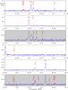 |
Fig. A.1 Detailed view of the observed spectrum of Orion KL at 7 mm (in blue), superimposed on the identification of the most intense lines and the best fit model for the molecular species (in red). Each panel displays a width of approximately 250 MHz. In order to improve the visibility of low intensity lines, some frequency ranges are plotted with a zoom in intensity (grey boxes); a second level of zoom, when necessary, is also depicted (yellow boxes). To compute the rest frequencies, a velocity of vLSR = +9 km s-1 is assumed. We note that the model results do not include the SiO masers nor the RRLs. |
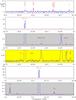 |
Fig. A.1 continued. |
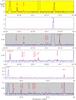 |
Fig. A.1 continued. |
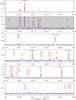 |
Fig. A.1 continued. |
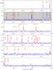 |
Fig. A.1 continued. |
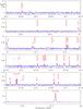 |
Fig. A.1 continued. |
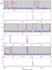 |
Fig. A.1 continued. |
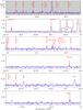 |
Fig. A.1 continued. |
Radio recombination lines detected.
LSR velocities of Hα RRLs in Orion KL.
Physical parameters derived by the models.
All Tables
All Figures
|
Fig. 1 Spectrum of Orion KL. Top panel: full range. Middle panel: magnification in intensity to see low intensity lines; green boxes are expanded in the three bottom panels, to show spectroscopic details. Some of the most intense lines are labelled. |
| In the text | |
|
Fig. 2 Distribution of the velocities of the RRLs as a function of frequency. Atoms (hydrogen, helium, and carbon) are labelled in red, blue, and green, respectively. |
| In the text | |
|
Fig. 3 LSR velocities of α RRLs from hydrogen in Orion KL, as a function of the frequency (on a logarithmic scale). Surveys used are indicated with different colours. Together with the references, the principal quantum numbers are indicated within parenthesis. Error bars correspond to 2σ values. |
| In the text | |
|
Fig. 4 Distribution of the measured line intensity ratios between pairs of hydrogen RRLs at nearby frequencies as a function of the predicted ratios under LTE conditions. The ratios are labelled and the bars represent 1.5σ errors. The dotted blue line corresponds to equal values between observed and predicted ratios under LTE conditions. |
| In the text | |
|
Fig. 5 The SiO J = 1 → 0 lines detected in Orion KL. Isotopologues and vibrational numbers are indicated in each panel. |
| In the text | |
|
Fig. A.1 Detailed view of the observed spectrum of Orion KL at 7 mm (in blue), superimposed on the identification of the most intense lines and the best fit model for the molecular species (in red). Each panel displays a width of approximately 250 MHz. In order to improve the visibility of low intensity lines, some frequency ranges are plotted with a zoom in intensity (grey boxes); a second level of zoom, when necessary, is also depicted (yellow boxes). To compute the rest frequencies, a velocity of vLSR = +9 km s-1 is assumed. We note that the model results do not include the SiO masers nor the RRLs. |
| In the text | |
|
Fig. A.1 continued. |
| In the text | |
|
Fig. A.1 continued. |
| In the text | |
|
Fig. A.1 continued. |
| In the text | |
|
Fig. A.1 continued. |
| In the text | |
|
Fig. A.1 continued. |
| In the text | |
|
Fig. A.1 continued. |
| In the text | |
|
Fig. A.1 continued. |
| In the text | |
Current usage metrics show cumulative count of Article Views (full-text article views including HTML views, PDF and ePub downloads, according to the available data) and Abstracts Views on Vision4Press platform.
Data correspond to usage on the plateform after 2015. The current usage metrics is available 48-96 hours after online publication and is updated daily on week days.
Initial download of the metrics may take a while.