| Issue |
A&A
Volume 603, July 2017
|
|
|---|---|---|
| Article Number | A122 | |
| Number of page(s) | 26 | |
| Section | Cosmology (including clusters of galaxies) | |
| DOI | https://doi.org/10.1051/0004-6361/201630349 | |
| Published online | 19 July 2017 | |
Sardinia Radio Telescope observations of Abell 194
The intra-cluster magnetic field power spectrum
1 INAF–Osservatorio Astronomico di Cagliari via della Scienza 5, 09047 Selargius (CA), Italy
e-mail: This email address is being protected from spambots. You need JavaScript enabled to view it.
2 Dip. di Fisica, Università degli Studi di Cagliari, Strada Prov.le Monserrato-Sestu Km 0.700, 09042 Monserrato (CA), Italy
3 Dip. di Fisica, Università degli Studi di Trieste – Sezione di Astronomia, via Tiepolo 11, 34143 Trieste, Italy
4 INAF–Osservatorio Astronomico di Trieste, via Tiepolo 11, 34143 Trieste, Italy
5 INAF–IASF Milano, via Bassini 15, 20133 Milano, Italy
6 Dep. of Physics and Astronomy, University of California at Irvine, 4129 Frederick Reines Hall, Irvine, CA 92697-4575, USA
7 INAF–Istituto di Radioastronomia, Bologna via Gobetti 101, 40129 Bologna, Italy
8 Dip. di Fisica e Astronomia, Università degli Studi di Bologna, Viale Berti Pichat 6/2, 40127 Bologna, Italy
9 Agenzia Spaziale Italiana (ASI), 00100 Roma, Italy
10 SKA SA, 3rd Floor, The Park, Park Road, 7405 Pinelands, The Cape Town, South Africa
11 Department of Physics and Electronics, Rhodes University, PO Box 94, 6140 Grahamstown, South Africa
12 Hamburger Sternwarte, Universität Hamburg, Gojenbergsweg 112, 21029 Hamburg, Germany
13 Fundación G. Galilei – INAF TNG, Rambla J. A. Fernández Pérez 7, 38712 Breña Baja (La Palma), Spain
14 Instituto de Astrofísica de Canarias, C/Vía Láctea s/n, 38205 La Laguna (Tenerife), Spain
15 Dep. de Astrofísica, Univ. de La Laguna, Av. del Astrofísico Francisco Sánchez s/n, 38205 La Laguna (Tenerife), Spain
16 ASTRON, the Netherlands Institute for Radio Astronomy, Postbus 2, 7990 AA, Dwingeloo, The Netherlands
17 Kapteyn Astronomical Institute, Rijksuniversiteit Groningen, Landleven 12, 9747 AD Groningen, The Netherlands
18 Naval Research Laboratory, Washington, District of Columbia 20375, USA
19 School of Physics, University of the Witwatersrand, Private Bag 3, 2050 Johannesburg, South Africa
20 University of Leiden, Rapenburg 70, 2311 EZ Leiden, The Netherlands
21 Astronomy Department, University of Geneva, 16 Ch. d’Ecogia, 1290 Versoix, Switzerland
22 Max Planck Institut für Astrophysik, Karl-Schwarzschild-Str.1, 85740 Garching, Germany
23 Laboratoire Lagrange, UCA, OCA, CNRS, Bd de l’Observatoire, CS 34229, 06304 Nice Cedex 4, France
24 School of Chemical & Physical Sciences, Victoria University of Wellington, PO Box 600, 6140 Wellington, New Zealand
25 Argelander-Institut für Astronomie, Auf dem Hügel 71, 53121 Bonn, Germany
26 National Radio Astronomy Observatory, PO Box O, Socorro, NM 87801, USA
27 Department of Physics and Astronomy, University of New Mexico, Albuquerque, NM 87131, USA
Received: 23 December 2016
Accepted: 23 March 2017
Abstract
Aims. We study the intra-cluster magnetic field in the poor galaxy cluster Abell 194 by complementing radio data, at different frequencies, with data in the optical and X-ray bands.
Methods. We analyzed new total intensity and polarization observations of Abell 194 obtained with the Sardinia Radio Telescope (SRT). We used the SRT data in combination with archival Very Large Array observations to derive both the spectral aging and rotation measure (RM) images of the radio galaxies 3C 40A and 3C 40B embedded in Abell 194. To obtain new additional insights into the cluster structure, we investigated the redshifts of 1893 galaxies, resulting in a sample of 143 fiducial cluster members. We analyzed the available ROSAT and Chandra observations to measure the electron density profile of the galaxy cluster.
Results. The optical analysis indicates that Abell 194 does not show a major and recent cluster merger, but rather agrees with a scenario of accretion of small groups, mainly along the NE−SW direction. Under the minimum energy assumption, the lifetimes of synchrotron electrons in 3C 40 B measured from the spectral break are found to be 157 ± 11 Myr. The break frequency image and the electron density profile inferred from the X-ray emission are used in combination with the RM data to constrain the intra-cluster magnetic field power spectrum. By assuming a Kolmogorov power-law power spectrum with a minimum scale of fluctuations of Λmin = 1 kpc, we find that the RM data in Abell 194 are well described by a magnetic field with a maximum scale of fluctuations of Λmax = (64 ± 24) kpc. We find a central magnetic field strength of ⟨ B0 ⟩ = (1.5 ± 0.2) μG, which is the lowest ever measured so far in galaxy clusters based on Faraday rotation analysis. Further out, the field decreases with the radius following the gas density to the power of η = 1.1 ± 0.2. Comparing Abell 194 with a small sample of galaxy clusters, there is a hint of a trend between central electron densities and magnetic field strengths.
Key words: galaxies: clusters: general / galaxies: clusters: individual: Abell 194 / magnetic fields / large-scale structure of Universe
© ESO, 2017
1. Introduction
Galaxy clusters are unique laboratories for the investigation of turbulent fluid motions and large-scale magnetic fields (e.g., Carilli & Taylor 2002; Govoni & Feretti 2004; Murgia 2011). In the last few years, several efforts have been focused on determining the effective strength and structure of magnetic fields in galaxy clusters and this topic represents a key project in view of the Square Kilometre Array (e.g., Johnston-Hollitt et al. 2015).
Synchrotron radio halos at the center of galaxy clusters (e.g., Feretti et al. 2012; Ferrari et al. 2008) provide direct evidence of the presence of relativistic particles and magnetic fields associated with intra-cluster medium. In particular, the detection of polarized emission from radio halos is key to investigating the magnetic field power spectrum in galaxy clusters (Murgia et al. 2004; Govoni et al. 2006, 2013, 2015; Vacca et al. 2010). However, detecting this polarized signal is a very hard task with current radio facilities and so far only three examples of large-scale filamentary polarized structures have been detected that are possibly associated with halo emission (A2255; Govoni et al. 2005; Pizzo et al. 2011, MACS J0717.5+3745; Bonafede et al. 2009; A523; Girardi et al. 2016).
Highly polarized elongated radio sources named relics are also observed at the periphery of merging systems (e.g., Clarke & Ensslin 2006; Bonafede et al. 2009b; van Weeren et al. 2010). These radio sources trace the regions where the propagation of mildly supersonic shock waves compresses the turbulent intra-cluster magnetic field, thereby enhancing the polarized emission and accelerating the relativistic electrons responsible for the synchrotron emission.
A complementary set of information on galaxy cluster magnetic fields can be obtained from high quality rotation measure (RM) images of powerful and extended radio galaxies. The presence of a magnetized plasma between an observer and a radio source changes the properties of the incoming polarized emission. In particular, the position angle of the linearly polarized radiation rotates by an amount that is proportional to the line integral of the magnetic field along the line-of-sight times the electron density of the intervening medium, i.e., the so-called Faraday rotation effect. Therefore, information on the intra-cluster magnetic fields can be obtained, in conjunction with X-ray observations of the hot gas, through the analysis of the RM of radio galaxies in the background or in the galaxy clusters themselves. Rotation measure studies have been performed on statistical samples (e.g., Clarke et al. 2001; Johnston-Hollitt & Ekers 2004; Govoni et al. 2010) as well as individual clusters (e.g., Perley & Taylor 1991; Taylor & Perley 1993; Feretti et al. 1995, 1999; Taylor et al. 2001; Eilek & Owen 2002; Pratley et al. 2013). These studies reveal that magnetic fields are widespread in the intra-cluster medium, regardless of the presence of a diffuse radio halo emission.
The RM distribution seen over extended radio galaxies is generally patchy, indicating that magnetic fields are not regularly ordered on cluster scales, but instead they have turbulent structures down to linear scales as small as a few kpc or less. Therefore, RM measurements probe the complex topology of the cluster magnetic field and indeed state-of-the-art software tools and approaches based on a Fourier domain formulation have been developed to constrain the magnetic field power spectrum parameters on the basis of the RM images (Enßlin & Vogt 2003; Murgia et al. 2004; Laing et al. 2008; Kuchar & Enßlin 2011; Bonafede et al. 2013). The magnetic field power spectrum has been estimated in some galaxy clusters and galaxy groups containing radio sources with very detailed RM images (e.g., Vogt & Enßlin 2003; Murgia et al. 2004; Vogt & Enßlin 2005; Govoni et al. 2006; Guidetti et al. 2008; Laing et al. 2008; Guidetti et al. 2010; Bonafede et al. 2010; Vacca et al. 2012). RM data are usually consistent with volume averaged magnetic fields of ≃0.1–1 μG over 1 Mpc3. The central magnetic field strengths are typically a few μG, but stronger fields, with values exceeding ≃10 μG, are measured in the inner regions of relaxed cooling core clusters. There are several indications that the magnetic field intensity decreases going from the center to the periphery following the cluster gas density profile. This has been illustrated by magneto-hydrodynamical simulations (see, e.g., Dolag et al. 2002; Brüggen et al. 2005; Xu et al. 2012; Vazza et al. 2014) and confirmed in RM data.
In this paper we aim at improving our knowledge of the intra-cluster magnetic field in Abell 194. This nearby (z = 0.018; Struble & Rood 1999) and poor (richness class R = 0; Abell et al. 1989) galaxy cluster belongs to the Sardinia Radio Telescope (SRT) Multifrequency Observations of Galaxy clusters (SMOG) sample, an early science program of the new SRT radio telescope. For our purpose, we investigated the total intensity and polarization properties of two extended radio galaxies embedded in Abell 194 in combination with data in optical and X-ray bands. The paper is organized as follows. In Sect. 2, we describe the SMOG project. In Sect. 3, we present the radio observations and data reduction. In Sect. 4, we present the radio, optical, and X-ray properties of Abell 194. In Sect. 5, we complement the SRT total intensity data with archival VLA observations to derive spectral aging information of the radio galaxies. In Sect. 6, we complement the SRT polarization data with archival VLA observations to derive detailed multiresolution RM images. In Sect. 7, we use numerical simulations to investigate the cluster magnetic field by analyzing the RM and polarization data. Finally, in Sect. 8 we summarize our conclusions.
Throughout this paper we assume a ΛCDM cosmology with H0 = 71 km s-1 Mpc-1, Ωm = 0.27, and ΩΛ = 0.73. At the distance of Abell 194, 1′′ corresponds to 0.36 kpc.
2. SRT Multifrequency observations of Galaxy clusters
Details of the SRT observations centered on Abell 194.
The SRT is a new 64 m single dish radio telescope located north of Cagliari, Italy. In its first light configuration, the SRT is equipped with three receivers: a 7-beam K-band receiver (18−26 GHz), a mono-feed C-band receiver (5700−7700 GHz), and a coaxial dual-feed L/P-band receiver (305−410 MHz, 1300−1800 MHz).
The antenna was officially opened on 30 September 2013, upon completion of the technical commissioning phase (Bolli et al. 2015). The scientific commissioning of the SRT was carried out in the period 2012–2015 (Prandoni et al. 2017). At the beginning of 2016 the first call for single dish early science programs was issued, and the observations started on February 1st, 2016.
The SMOG project is an SRT early science program (PI M. Murgia) focused on a wide-band and wide-field single dish spectral-polarimetric study of a sample of galaxy clusters. By comparing and complementing the SRT observations with archival radio data at higher resolution and at different frequencies, but also with data in optical and X-ray bands, we want to improve our knowledge of the non-thermal components of the intra-cluster medium on a large scale. Our aim is also to understand the interplay between these components (relativistic particles and magnetic fields) and the life cycles of cluster radio galaxies by studying both the spectral and polarization properties of the radio sources with the SRT (see, e.g., the case of 3C 129; Murgia et al. 2016). For this purpose, we selected a suitable sample of nearby galaxy clusters known from the literature to harbor diffuse radio halos, relics, or extended radio galaxies.
We included Abell 194 in the SMOG sample because it is one of the rare clusters hosting more than one luminous and extended radio galaxy close to the cluster center. In particular, it hosts the radio source 3C 40 (PKS 0123-016), which is indeed constituted by two radio galaxies with distorted morphologies (3C 40A and 3C 40B). This galaxy cluster has been extensively analyzed in the literature with radio interferometers (e.g., O’Dea & Owen 1985; Jetha et al. 2006; Sakelliou et al. 2008; Bogdán et al. 2011). Here we present, for the first time, total intensity and polarization single-dish observations obtained with the SRT at 6600 MHz. The importance of mapping the radio galaxies in Abell 194 with a single dish is that interferometers suffer the technical problem of not measuring the total power; the so-called missing zero spacing problem. Indeed, they filter out structures larger than the angular size corresponding to their shortest spacing, thus limiting the synthesis imaging of extended structures. Single dish telescopes are optimal for recovering all of the emission on large angular scales, especially at high frequencies (>1 GHz). Although single dishes typically have a low resolution, the radio galaxies at the center of Abell 194 are sufficiently extended to be well resolved with the SRT at 6600 MHz at the resolution of 2.9′.
The SRT data at 6600 MHz are used in combination with archival Very Large Array observations at lower frequencies to derive the trend of the synchrotron spectra along 3C 40A and 3C 40B. In addition, linearly polarized emission is clearly detected for both sources and the resulting polarization angle images are used to produce detailed RM images at different angular resolutions. 3C 40B and 3C 40A are very extended both in angular and linear size, therefore they represent ideal cases for studying the RM of the cluster along different lines of sight. In addition, the close distance of Abell 194 permits a detailed investigation of the cluster magnetic field structure. Following Murgia et al. (2004), we simulated Gaussian random magnetic field models and we compared the observed data and the synthetic images with a Bayesian approach (Vogt & Enßlin 2005) to constrain the strength and structure of the magnetic field associated with the intra-cluster medium. Until recently, most of the work on cluster magnetic fields has been devoted to rich galaxy clusters. Little attention has been given in the literature to magnetic fields associated with poor galaxy clusters such as Abell 194 and galaxy groups (see, e.g., Laing 2008; Guidetti et al. 2008, 2010). Magnetic fields in these systems deserve to be investigated in detail since, being more numerous, are more representative than those of rich clusters.
Details of VLA archival observations of Abell 194 analyzed in this paper.
3. Radio observations and data reduction
3.1. SRT observations
We observed with the SRT, for a total exposure time of about 14.4 h, an area of 1 deg × 1 deg centered on the galaxy cluster Abell 194 using the C-band receiver. Full-Stokes parameters were acquired with the SARDARA backend (SArdinia Roach2-based Digital Architecture for Radio Astronomy; Melis et al. 2017), which is one of the backends available at the SRT (Melis et al. 2014). We used the correlator configuration with 1500 MHz and 1024 frequency channels of approximately 1.46 MHz in width. We observed in the frequency range 6000−7200 MHz at a central frequency of 6600 MHz. We performed several on-the-fly (OTF) mappings in the equatorial frame alternating the right ascension (RA) and declination (Dec). The telescope scanning speed was set to 6 arcmin/s and the scans were separated by 0.7′ to properly sample the SRT beam whose full width at half maximum (FWHM) is 2.9′ in this frequency range. We recorded the data stream sampling at 33 spectra per second, therefore individual samples were separated on the sky by 10.9′′ along the scanning direction. A summary of the SRT observations is listed in Table 1. Data reduction was performed with the proprietary Single-dish Spectral-polarimetry Software (SCUBE; Murgia et al. 2016).
Bandpass, flux density, and polarization calibration were carried out with at least four cross scans on source calibrators performed at the beginning and at the end of each observing section.
Bandpass and flux density calibration were performed by observing 3C 286 and 3C 138, assuming the flux density scale of Perley & Butler (2013). After a first bandpass and flux density calibration cycle, persistent radio frequency interference (RFI) were flagged using observations of a cold part of the sky. The flagged data were then used to repeat the bandpass and flux density calibration for a finer RFI flagging. The procedure was iterated a few times, eliminating all of the most obvious RFI. We applied the gain-elevation curve correction to account for the gain variation with elevation due to the telescope structure gravitational stress change.
We performed the polarization calibration by correcting the instrumental polarization and the absolute polarization angle. The on-axis instrumental polarization was determined through observations of the bright unpolarized source 3C 84. The leakage of Stokes I into Q and U is in general less than 2% across the band with a rms scatter of 0.7–0.8%. We fixed the absolute position of the polarization angle using as reference the primary polarization calibrator 3C 286 and 3C 138. The difference between the observed and predicted position angle according to Perley & Butler (2013) was determined and corrected channel by channel. The calibrated position angle was within the expected value of 33° and −11.9° for 3C 286 and 3C 138, respectively, with a rms scatter of ±1°.
In the following we describe the total intensity and polarization imaging. For further details on the calibration and data handling of the SRT observations, see Murgia et al. (2016).
3.1.1. Total intensity imaging
The imaging was performed in SCUBE by subtracting the baseline from the calibrated telescope scans and by projecting the data in a regular three-dimensional grid. At 6600 MHz we used a spatial resolution of 0.7′/pixel (corresponding to the separation of the telescope scans), which is enough in our case to sample the beam FWHM with four pixels.
As a first step, the baseline was subtracted by a linear fit involving only the 10% of data at the beginning and end of each scan. The baseline removal was performed channel by channel for each scan. All frequency cubes obtained by gridding the scans along the two orthogonal axes (RA and Dec) were then stacked together to produce full-Stokes I, Q, U images of an area of 1 square degree centered on the galaxy cluster Abell 194. In the combination, the individual image cubes were averaged and destripped by mixing their Stationary Wavelet Transform (SWT) coefficients (see Murgia et al. 2016, for details). We then used the higher signal-to-noise (S/N) image cubes obtained from the SWT stacking as a prior model to refine the baseline fit. The baseline subtraction procedure was then repeated including not just the 10% from the begin and the end of each scan. In the refinement stage, the baseline was represented with a 2nd order polynomial using the regions of the scans free of radio sources. A new SWT stacking was then performed and the process was iterated a few more times until the convergence was reached.
Close to the cluster center, the dynamical range of the C-band total intensity image was limited by the telescope beam pattern rather than by the image sensitivity. In SCUBE, we used a beam model pattern (Murgia et al. 2016) for a proper deconvolution of the sky image from the antenna pattern. The deconvolution algorithm interactively finds the peak in the image obtained from the SWT stacking of all images and subtracts a fixed gain fraction (typically 0.1) of this point source flux convolved with the reprojected telescope “dirty beam model” from the individual images. In the reprojection, the exact elevation and parallactic angle for each pixel in the unstacked images are used. The residual images were stacked again and the CLEAN continued until a threshold condition was reached. Given the low level of the beam side lobes compared to interferometric images, a shallow deconvolution was sufficient in our case, and we decided to stop the CLEAN at the first negative component encountered. As a final step, CLEAN components at the same position were merged, smoothed with a circular Gaussian beam with FWHM 2.9′, and then restored back in the residuals image to obtain a CLEANed image.
3.1.2. Polarization imaging
The polarization imaging at C band of Stokes parameters Q and U was performed following the same procedures described for the total intensity imaging: baseline subtraction, gridding, and SWT stacking. There were no critical dynamic range issues with the polarization image, and thus no deconvolution was required. However, since the contribution of the off-axis instrumental polarization can affect the quality of polarization data if bright sources are present in the image, we corrected for the off-axis instrumental polarization by deconvolving the Stokes Q and U beam patterns. In particular, SCUBE uses the CLEAN components derived from the deconvolution of the beam pattern from the total intensity image to subtract the spurious off-axis polarization from each individual Q and U scans before their stacking. The off-axis instrumental polarization level compared to the Stokes I peak is 0.3%.
Finally, polarized intensity  (corrected for the positive bias), fractional polarization FPOL = P / I, and position angle of polarization Ψ = 0.5tan-1(U/Q) images were then derived from the I, Q, and U images.
3.2. Archival VLA observations
We analyzed archival observations obtained with the VLA at different frequencies and configurations. The details of the observations are provided in Table 2. The data were reduced using the NRAO Astronomical Image Processing System (AIPS) package.
The data in C band and in L band were calibrated in amplitude, phase, and polarization angle using the standard calibration procedure. The flux density of the calibrators were calculated accordingly to the flux density scale of Perley & Butler (2013). Phase calibration was derived from nearby sources, which were periodically observed over a wide range in parallactic angle. The radio sources 3C 286 or 3C 138 were used as reference for the absolute polarization angles. Phase calibrators were also used to separate the source polarization properties from the antenna polarizations. Imaging was performed following the standard procedure: Fourier transform, clean, and restore. A few cycles of self-calibration were applied when proven to be useful to remove residual phase variations. Images of the Stokes parameters I, Q, and U were produced for each frequency and configuration separately providing different angular resolutions. Since the C-band data consist of three separate short pointings, in this case, the final I, Q, and U images were obtained by mosaicking the three different pointings with the AIPS task FLATN. Finally, P, FPOL, and Ψ images were then derived from the I, Q, and U images.
Data in P band were obtained in spectral line mode dividing the bandwidth of 3.125 MHz in 31 channels. We edited the data to excise RFI channel by channel. We performed the amplitude and bandpass calibration with the source 3C 48. The flux density of the calibrator was calculated accordingly to the low frequency coefficients of Scaife & Heald (2012). In the imaging, the data were averaged into five channels. The data were mapped using a wide-field imaging technique, which corrects for distortions in the image caused by the non-coplanarity of the VLA over a wide field of view. A set of small overlapping maps was used to cover the central area of about ~2.4° in radius (Cornwell & Perley 1992). However, at this frequency confusion lobes of sources far from the center of the field are still present. Thus, we also obtained images of strong sources in an area of about ~6° in radius, searched in the NRAO VLA Sky Survey (NVSS; Condon et al. 1998) catalog. All these “facets” were included in CLEAN and used for several loops of phase self-calibration (Perley 1999). To improve the u-v coverage and sensitivity we combined the data sets in B and C configuration.
4. Multiwavelengths properties of Abell 194
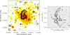 |
Fig. 1 Left: SRT radio image at 6600 MHz (contours) overlaid on the ROSAT PSPC X-ray image (colors) in the 0.4–2 keV band. The SRT image results from the spectral average of the bandwidth between 6000 and 7200 MHz. It has a sensitivity of 1 mJy/beam and an angular resolution of 2.9′. The first radio contour is drawn at 3 mJy/beam (3σI) and the rest are spaced by a factor of |

In the following we present the radio, optical, and X-ray properties of the galaxy cluster Abell 194.
4.1. Radio properties
In Fig. 1, we show the radio, optical, and X-ray emission of Abell 194. The field of view of the left panel of Fig. 1 is ≃1.3 × 1.3 Mpc2. In this panel, the contours of the CLEANed radio image obtained with the SRT at 6600 MHz are overlaid on the X-ray ROSAT PSPC image in the 0.4–2 keV band (see Sect. 4.3). The SRT image was obtained by averaging all the frequency channels from 6000 MHz to 7200 MHz. We reached a final noise level of 1 mJy/beam and an angular resolution of 2.9′ FWHM. The radio galaxy 3C 40B, close to the cluster X-ray center, extends for about 20′. The peak brightness of 3C 40B (≃600 mJy/beam) is located in the southern lobe. The narrow angle-tail radio galaxy 3C 40A (peak brightness ≃150 mJy/beam) is only slightly resolved at the SRT resolution and it is not clearly separated from 3C 40B.
The details of the morphology of the two radio galaxies can be appreciated in the right panel of Fig. 1, where we show a field of view of ≃0.5 × 0.5 Mpc2. In this panel, the contours of the radio image obtained with the VLA at 1443 MHz are overlaid on the optical emission of the cluster. We retrieved the optical image in the gMega band from the CADC Megapipe1 archive (Gwyn 2008). The VLA radio image was obtained from the L band data set in C configuration. It has a sensitivity of 0.34 mJy/beam and an angular resolution of 19′′. The distorted morphology of the two radio galaxies 3C 40B and 3C 40A is well visible. Both radio galaxies show an optical counterpart and their host galaxies are separated by 4.6′ (≃100 kpc). The core of the extended source 3C 40B is associated with NGC 547, which is known to form a dumbbell system with the galaxy NGC 545 (e.g. Fasano et al. 1996). 3C 40A is a narrow angle-tail radio galaxy associated with the galaxy NGC 541 (O’Dea & Owen 1985). The jet emanating from 3C 40A is believed to be responsible for triggering star formation in Minkowski’s object (e.g., van Breugel et al. 1985; Brodie et al. 1985; Croft et al. 2006), which is a star-forming peculiar galaxy near NGC 541.
Flux density measurements of faint radio sources detected in the Abell 194 field.
In addition to 3C 40A and 3C 40B, some other faint radio sources were detected in the Abell 194 field. In the left panel of Fig. 1, SRT sources with an NVSS counterpart are labeled with the letters A to S. Sources labeled with E, J, and Q are actually blends of multiple NVSS sources. There are also a few sources visible in the NVSS but not detected at the sensitivity level of the SRT image. These are likely steep spectral index radio sources. The SRT contours show an elongation in the northern lobe of 3C 40B toward the west. This elongation is likely due to the point source labeled with S, which is detected both in the 1443 MHz VLA image at 19′′ resolution in the right panel of Fig. 1, and in the NVSS. The 1443 MHz image also shows the presence of another point source located on the east of the northern lobe of 3C 40B. This point source is blended with 3C 40B both at the SRT and at the NVSS resolution.
Given that 3C 40A and 3C 40B are not clearly separated at the SRT resolution, we calculated the flux density for the two sources together by integrating the total intensity image at 6600 MHz down to the 3σI isophote. It results ≃1.72 ± 0.05 Jy. This flux also contains the flux of the two discrete sources located in the northern lobe of 3C 40B mentioned above.
In Table 3, we list the basic properties of the faint radio sources detected in the field of the SRT image. For the unresolved sources, we calculated the flux density by means of a two-dimensional Gaussian fit. Along with the SRT coordinates and the SRT flux densities, we also report their NVSS name, the NVSS flux density at 1400 MHz, and the global spectral indices (Sν ∝ ν− α) between 1400 and 6600 MHz.
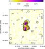 |
Fig. 2 SRT linearly polarized intensity image at 6600 MHz of the galaxy cluster Abell 194, resulting from the spectral average of the bandwidth between 6000 and 7200 MHz. The noise level, after the correction for the polarization bias, is σP = 0.5 mJy/beam. The FWHM beam is 2.9′, as indicated in the bottom left corner. Contours refer to the total intensity image. Levels start at 3 mJy/beam (3σI) and increase by a factor of 2. The electric field (E-field) polarization vectors are only traced for those pixels where the total intensity signal is above 5σI, the error on the polarization angle is less than 10°, and the fractional polarization is above 3σFPOL. The length of the vectors is proportional to the polarization percentage (with 100% represented by the bar in the top left corner). |
In Fig. 2, we show the total intensity SRT contours levels overlaid on the linearly polarized intensity image P at 6600 MHz. The polarized intensity was corrected for both the on-axis and off-axis instrumental polarization. The noise level, after the correction for the polarization bias, is σP = 0.5 mJy/beam. Polarization is detected for both 3C 40B and 3C 40A with a global fractional polarization of ≃9%. The peak polarized intensity is of ≃19 mJy/beam, located in the south lobe of 3C 40B, not matching the total intensity peak. The origin of this mismatch could be attributed to different effects. A possibility is that the magnetic field inside the lobe of the radio source is not completely ordered. Indeed, along the line of sight at the position of the peak intensity, we may have by chance two (or more) magnetic field structures that are not perfectly aligned in the plane of the sky so that the polarized intensity is reduced, while the total intensity is unaffected. This depolarization is a pure geometrical effect related to the intrinsic ordering of the magnetic field of the source and may be present even if there is no Faraday rotation inside and/or outside the radio emitting plasma. Another possibility is that Faraday rotation is occurring in an external screen and the peak intensity is located in projection in a region of a high RM gradient (see RM image in Fig. 8). In this case, the beam depolarization is expected to reduce the polarized signal but not the total intensity. Finally, there could be also internal Faraday rotation, but the presence of an X-ray cavity (see Sect. 4.3) suggests that the southern lobe is devoid of thermal gas and, furthermore, the observed trend of the polarized angles are consistent with the λ2 law that points in favor of an external Faraday screen (see Sect. 6).
In 3C 40B the fractional polarization increases along the source from 1–3% in the central brighter part up to 15–18% in the low surface brightness associated with the northern lobe. The other faint sources detected in the Abell 194 field are not significantly polarized in the SRT image.
4.2. Optical properties
One of the intriguing properties of Abell 194 is that it appears as a “linear cluster”, as its galaxy distribution and X-ray emission are both linearly elongated along the NE−SW direction (Rood & Sastry 1971; Struble & Rood 1987; Chapman et al. 1988; Nikogossyan et al. 1999; Jones & Forman 1999).
Previous studies of Abell 194, based on redshift data, have found a low value of the velocity dispersion of galaxies within the cluster (~350−400 km s-1; Chapman et al. 1988; Girardi et al. 1998) and a low value of the mass. Two independent analyses agree in determining a mass of M200 ~ 1 × 10¹⁴h-1M⊙within the radius2R200 ~ 1 Mpc (Girardi et al. 1998; Rines et al. 2003). Early analyses of redshift data samples of ~100–150 galaxies within 3–6 Mpc, mostly derived by Chapman et al. (1988), confirmed that Abell 194 is formed of a main system elongated along the NE−SW direction and detected minor substructure in both the central and external cluster regions (Girardi et al. 1997; Barton et al. 1998; Nikogossyan et al. 1999).
To obtain new additional insights into the cluster structure, we considered more recent redshift data. Rines et al. (2003) compiled redshifts from the literature as collected by the NASA/IPAC Extragalactic Database (NED), including the first Sloan Digital Sky Survey (SDSS) data. Here, we also added further data extracted from the last SDSS release (DR12). In particular, to analyze the 2R200 cluster region, we considered galaxies within 2 Mpc (~93′) from the cluster center (here taken as the galaxy 3C 40B/NGC 547). Our galaxy sample consists of 1893 galaxies. After the application of the P+G membership selection (Fadda et al. 1996; Girardi et al. 2015) we obtained a sample of 143 fiducial members. The P+G membership selection is a two-step method. First, we used the one-dimensional adaptive-kernel method DEDICA (Pisani 1993) to detect the significant cluster peak in the velocity distribution. All the galaxies assigned to the cluster peak are analyzed in the second step, which uses a combination of position and velocity information, i.e., the “shifting gapper” method by Fadda et al. (1996). This procedure rejects galaxies that are too far in velocity from the main body of galaxies and within a fixed bin that shifts along the distance from the cluster center. The procedure is iterated until the number of cluster members converges to a stable value.
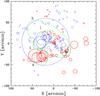 |
Fig. 3 Spatial distribution of the 143 cluster member galaxies. The larger the circle, the larger is the deviation of the local mean velocity, as computed on the galaxy and its 10 neighbors, from the global mean velocity. The blue thin-line and red thick-line circles show where the local value of mean velocity is lower or higher than the global value. The green dashed ellipses indicate the regions of the subgroups detected by Nikogossyan et al. (1999; see their Fig. 13, the subgroup No. 2 is outside of our field). The center is fixed on the NGC 547 galaxy. |
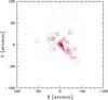 |
Fig. 4 Spatial distribution of the 143 cluster members (small black points). The galaxies of the two main subgroups detected in the 3D-DEDICA analysis are indicated by large symbols. The red squares and blue rotated squares indicate galaxies of the main and secondary subgroups, respectively. The secondary subgroup is characterized by a lower velocity. The larger the symbol size, the larger is the deviation of the galaxy from the mean velocity. The center is fixed on the NGC 547 galaxy (large black circle). NGC 545 and NGC 541 are indicated by small circles. |
The comparison with the corresponding galaxy samples of Chapman et al. (1988), which is formed of 84 galaxies (67 members), shows that we have doubled the data sample and stresses the difficulty of improving the Abell 194 sample when going down to fainter luminosities. Unlike the Chapman et al. (1988) sample, the sampling and completeness of both our sample and that of Rines et al. (2003) are not uniform and, in particular, since the center of Abell 194 is at the border of a SDSS strip, the southern cluster regions are undersampled with respect to the northern regions. As a consequence, we limited our analysis of substructure to the velocity distribution and to the position-velocity combined data.
By applying the biweight estimator to the 143 cluster members (Beers et al. 1990, ROSTAT software), we computed a mean cluster line-of-sight (LOS) velocity ⟨ V ⟩ = ⟨ cz ⟩ = (5375 ± 143) km s-1, corresponding to a mean cluster redshift ⟨ z ⟩ = 0.017929 ± 0.0004 and a LOS velocity dispersion  km s-1, in good agreement with the estimates by Rines et al. (2003, see their Table 2). There is no evidence of non-Gaussianity in the galaxy velocity distribution according to two robust shape estimators, the asymmetry index and tail index, and the scaled tail index (Bird & Beers 1993). We also verified that the three luminous galaxies in the cluster core (NGC 547, NGC 545, and NGC 541) have no evidence of peculiar velocity according to the indicator test by Gebhardt & Beers (1991).
We applied the Δ-statistics devised by Dressler & Schectman (1988; hereafter DS-test), which is a powerful test for three-dimensional substructure. The significance is based on 1000 Monte Carlo simulated clusters obtained shuffling galaxies velocities with respect to their positions. We detected a marginal evidence of substructure (at the 91.3% confidence level). Figure 3 shows the comparison of the DS bubble plot, here obtained considering only the local velocity kinematical DS indicator, with the subgroups detected by Nikogossyan et al. (1999). The most important subgroup detected by Nikogossyan et al. (1999), No. 3, traces the NE−SW elongated structure. Inside this, the regions characterized by low or high local velocity correspond to their No. 1 and No. 5 subgroups. A SE region characterized by a high local velocity corresponds to their No. 4 subgroup, the only one outside the main NE−SW cluster structure. The above agreement is particularly meaningful when considering that the Nikogossyan et al. (1999) and our results are based on quite different samples and analyses. In particular, their hierarchical-tree analysis weights galaxies with their luminosity, while no weight is applied in our DS test and plot. The galaxy with a very large blue thin-lined circle has a difference from the mean cz of 488 km s-1 and lies at 0.42 Mpc from the cluster center, which is well inside the caustic lines reported by Rines et al. (2003, see their Fig. 2) and thus it is definitely a cluster member. However, this galaxy lies at the center of a region inhabited by several galaxies at low velocity, resulting in the large size of the circle. In fact, as mentioned in the caption, the circle size refers to the local mean velocity as computed with respect to the galaxy and its 10 neighbors.
We also performed the three-dimensional optimized adaptive-kernel method of Pisani (1993, 1996; hereafter 3D-DEDICA; see also Girardi et al. 2016). The method detects two important density peaks, significant at the >99.99% confidence level of 31 and 15 galaxies. Minor subgroups have very low density and/or richness and are not discussed. Figure 4 shows that both the two DEDICA subgroups are strongly elongated and trace the NE−SW direction but have different velocities. The main subgroup has a velocity peak of 5463 km s-1, close to the mean cluster velocity, and contains NGC 547, NGC 545, and NGC 541. The secondary subgroup has a lower velocity (4897 km s-1).
The picture resulting from new and previous optical results agree in that Abell 194 does not show trace of a major and recent cluster merger (e.g., as in the case of a bimodal head-on merger), but rather agrees with a scenario of accretion of small groups, mainly along the NE−SW axis.
4.3. X-ray properties
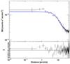 |
Fig. 5 Surface brightness profile of the X-ray emission of Abell 194. The profile is centered at the position of the X-ray centroid. The best fit β-model is shown in blue. |
The cluster Abell 194 has been observed in X-rays with the ASCA, ROSAT, Chandra, and XMM satellites. Sakelliou et al. (2008) investigated the cluster relying on XMM and radio observations. The X-ray data do not show any signs of features expected from recent cluster merger activity. They concluded that the central region of Abell 194 is relatively quiescent and does not suffer a major merger event, which is in agreement with the optical analysis described in Sect. 4.2. Bogdán et al. (2011) analyzed X-ray observations with Chandra and ROSAT satellites. These authors mapped the dynamics of the galaxy cluster and also detected a large X-ray cavity formed by the southern radio lobe arising from 3C 40B. Therefore, this target is particularly interesting for Faraday rotation studies because the presence of an X-ray cavity indicates that the rotation of the polarization plane is likely to occur entirely in the intra-cluster medium, since comparatively little thermal gas should be present inside the radio-emitting plasma.
The temperature profile and cooling time of 21.6 ± 4.41 Gyr determined by Lovisari et al. (2015) and the temperature map by Bogdán et al. (2011) indicate that Abell 194 does not harbor a cool core.
We analyzed the ROSAT PSPC pointed observation of Abell 194 following the same procedure of Eckert et al. (2012) to which we refer for a more detailed description. Here we briefly mention the main steps of the reduction and analysis. The ROSAT Extended Source Analysis Software (Snowden et al. 1994) was used for the data reduction. The contribution of the various background components, such as scattered solar X-rays, long-term enhancements, and particle background, has been taken into account and combined to get a map of all the non-cosmic background components to be subtracted. We then extracted the image in the R37 ROSAT energy band (0.4–2 keV) corrected for vignetting effect with the corresponding exposure map. We detected and excluded point sources up to a constant flux threshold to ensure a constant resolved fraction of the cosmic X-ray background (CXB) over the field of view. The surface brightness profile was computed with 30 arcsec bins centered on the centroid of the image (RA = 01 25 54; Dec = –01 21 05) out to 50 arcmin. The surface brightness profile was fitted with a single β-model (Cavaliere & Fusco-Femiano 1976) plus a constant (to take into account the sky background composed by Galactic foregrounds and residual CXB) with the software proffit v1.3 (Eckert et al. 2011). The best fitting model has a core radius rc = 11.5 ± 1.2 arcmin (248.4 ± 26 kpc) and β = 0.67 ± 0.06 (1σ) for a χ2/d.o.f. = 1.77. In Fig. 5 we show the surface brightness profile of the X-ray emission of Abell 194 with the best fit β-model shown in blue.
For the determination of the spectral parameters representative of the core properties, we analyzed the Chandra ACIS-S observation of Abell 194 (ObsID: 7823) with CIAO 4.7 and CALDB 4.6.8. All data were reprocessed from the level = 1 event file following the standard Chandra reduction threads and flare cleaning. We used blank-sky observations to subtract the background components and to account for variations in the normalization of the particle background we rescaled the blank-sky background template by the ratio of the count rates in the 10–12 keV energy band. We extracted a spectrum from a circular region of radius 1 arcmin around the centroid position. We fitted the data with an apec (Smith et al. 2001) model with ATOMDB code v2.0.2. in xspec v.12.8.2 (Arnaud 1996). We fixed the Galactic column density at NH = 4.11 × 1020 cm-2 (Kalberla et al. 2005); the abundance is quoted in the solar units of Anders & Grevesse (1989) and we used the Cash statistic. The best fit model gives a temperature of kT = 2.4 ± 0.3 keV, an abundance of  , and a xspec normalization of 1.0 ± 0.1 × 10⁻⁴ cm-5 for a cstat/d.o.f. = 82/83.
Using the ROSAT best fit β-model and the spectral parameters obtained with Chandra the central electron density can be expressed by a simple analytical formula (Eq. (2) of Ettori et al. 2004). In order to assess the error we repeated the measurements after 1000 random realizations of the normalization and the β-model parameters drawn from Gaussian distributions with mean and standard deviation set by the best fit results. We obtain a value for the central electron density of n0 = (6.9 ± 0.6) × 10-4 cm-3. The distribution of the thermal electrons density with the distance from the cluster X-ray center r was thus modeled with 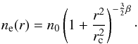 (1)
(1)
5. Spectral aging analysis
Relevant parameters of the images smoothed to a resolution of 174′′(2.9′) and 60′′.
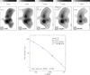 |
Fig. 6 Top: images of 3C 40A and 3C 40B at different frequencies, smoothed to a resolution of 2.9′. The images are VLSSr (74 MHz; Lane et al. 2014), VLA P band (330 MHz), VLA L band (1443 and 1630 MHz), and SRT (6600 MHz). The dynamic range (DR) of each image is shown on each of the top panels. Bottom: total spectrum of sources 3C 40 A and 3C 40 B together. The blue line is the best fit of the CI model. |
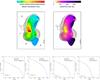 |
Fig. 7 Top left: map of break frequency, smoothed to a resolution of 2.9′, and derived with the pixel by pixel fit of the JP model in the regions where the brightness of the VLSSr image is above 5σI. In the break frequency image there are about 15 independent beams. Contours refer to the SRT image at 6600 MHz. Crosses indicate the optical core of 3C 40 A and 3C 40 B. Top right: map of the radiative age, smoothed to a resolution of 2.9′, and derived in Eq. (2) by applying the break frequency image and minimum energy magnetic field. In the radiative age image there are about 15 independent beams. Contours refer to the SRT image at 6600 MHz. Bottom: plots of the radio surface brightness as a function of the observing frequency ν at different locations. The resulting fit of the JP model is shown as a blue line. |
We investigated 3C 40A and 3C 40B at different frequencies to study their spectral index behavior in detail.
We analyzed the images obtained from the VLA Low-Frequency Sky Survey redux (VLSSr at 74 MHz; Lane et al. 2014), the VLA archive data in P band (330 MHz), the VLA archive data in L band (1443 and 1630 MHz), and the SRT (6600 MHz) data. We smoothed all the images to the same resolution as that of the SRT image (see top panels of Fig. 6). The relevant parameters of the images smoothed to a resolution of 2.9′ are reported in Table 4.
We calculated the flux densities of 3C 40 A and 3C 40 B together. The total spectrum of the sources is shown in the bottom panel of Fig. 6. Although the radio sources in Abell 194 have a large angular extension, the interferometric VLA data at 1443 and 1630 MHz do not seem to suffer from missing flux problem. To calculate the error associated with the flux densities, we added in quadrature the statistical noise and an additional uncertainty of 10% to take into account a different uv coverage and a possible bias due to the different flux density scale of the data sets.
We fitted the integrated spectrum with the continuous injection model (CI; Pacholczyk 1970) with the software SYNAGE (Murgia et al. 1999). The CI model is characterized by three free parameters: the injection spectral index (αinj), the break frequency (νb), and the flux normalization. In the context of the CI model, it is assumed that the spectral break is due to the energy losses of the relativistic electrons. For high-energy electrons, energy losses are primarily due to the synchrotron radiation itself and to inverse Compton scattering of cosmic microwave background (CMB) photons. During the active phase, the evolution of the integrated spectrum is determined by the shift with time of νb to lower and lower frequencies. Indeed, the spectral break can be considered to be a clock indicating the time elapsed since the injection of the first electron population. Below and above νb, the spectral indices are αinj and αinj + 0.5, respectively.
For 3C 40 A and 3C 40 B the best fit of the CI model to the observed radio spectrum yields a break frequency νb ≃ 700 ± 280 MHz. To limit the number of free parameters, we fixed αinj = 0.5, which is the value of the spectral index calculated in the jets of 3C 40B, at a relatively high resolution (≃20′′), between the L-band (1443 MHz) and the P-band (330 MHz) images.
We also studied the variation pixel by pixel of the synchrotron spectrum along 3C 40A and 3C 40B using the images in the top panels of Fig. 6. 3C 40B is extended enough to investigate the spectral trend along its length. A few plots showing the radio surface brightness as a function of the observing frequency at different locations of the 3C 40B are shown in bottom panels of Fig. 7. The plots show some pixels, located in different parts of 3C 40B, with representative spectral trend.
The morphology of the radio galaxy and the trend of the spectral curvatures at different locations indicate that 3C 40B is currently an active source whose synchrotron emission is dominated by electron populations with GeV energies injected by radio jets and accumulated during their entire lives (Murgia et al. 2011).
We then fitted the observed spectra with the JP model (Jaffe & Perola 1973), which also has three free parameters αinj, νb, and flux normalization as in the CI model. The JP model however describes the spectral shape of an isolated electron population with an isotropic distribution of the pitch angles injected at a specific instant in time with an initial power-law energy spectrum with index p = 2αinj + 1. According to the synchrotron theory (e.g., Blumenthal & Gould 1970; Rybicki & Lightman 1979), it is possible to relate the break frequency to the time elapsed since the start of the injection, ![Mathematical equation: \begin{equation} t_{\rm syn}= 1590 \frac{B^{0.5}}{(B^2+B_{\rm IC}^2) [(1+z)\nu_{\rm b}]^{0.5}}~\rm Myr, \label{synage} \end{equation}](/articles/aa/full_html/2017/07/aa30349-16/aa30349-16-eq141.png) (2)where B and BIC = 3.25(1 + z)2 are the source magnetic field and the inverse Compton equivalent magnetic field associated with the CMB, respectively. The resulting map of the break frequency derived by the fit of the JP model is shown in the top left panel of Fig. 7. The break frequency is computed in the regions where the brightness of the VLSSr image smoothed to a resolution of 2.9 is above 5σI (>1.3 Jy/beam). The measured break frequency decreases systematically along the lobes of 3C 40B in agreement with a scenario in which the oldest particles are those at larger distance from the AGN. The minimum break frequency measured in the faintest part of the lobes of 3C 40B is νb ≃ 850 ± 120 MHz, in agreement, within the errors, with the spectral break measured in the integrated spectrum of 3C 40 A and 3C 40 B.
(2)where B and BIC = 3.25(1 + z)2 are the source magnetic field and the inverse Compton equivalent magnetic field associated with the CMB, respectively. The resulting map of the break frequency derived by the fit of the JP model is shown in the top left panel of Fig. 7. The break frequency is computed in the regions where the brightness of the VLSSr image smoothed to a resolution of 2.9 is above 5σI (>1.3 Jy/beam). The measured break frequency decreases systematically along the lobes of 3C 40B in agreement with a scenario in which the oldest particles are those at larger distance from the AGN. The minimum break frequency measured in the faintest part of the lobes of 3C 40B is νb ≃ 850 ± 120 MHz, in agreement, within the errors, with the spectral break measured in the integrated spectrum of 3C 40 A and 3C 40 B.
We derived the radiative age from Eq. (2) using the minimum energy magnetic field strength. The minimum energy magnetic field was calculated assuming, for the electron energy spectrum, a power law with index p = 2αinj + 1 = 2 and a low energy cutoff at a Lorentz factor γlow = 100. In addition, we assumed that non-radiating relativistic ions have the same energy density as the relativistic electrons. We used the luminosity at 330 MHz, since radiative losses are less important at low frequencies. Modeling the lobes of 3C 40B as two cylinders in the plane of the sky, the resulting minimum energy magnetic field is ≃1.8 μG in the northern lobe and ≃1.7 μG in the southern lobe. Assuming ⟨ Bmin ⟩ = 1.75 μG for the magnetic field of the source and the lowest measured break frequency of νb = 850 ± 120 MHz, the radiative age of 3C 40B is found to be tsyn = 157 ± 11 Myr. Sakelliou et al. (2008) applied a similar approach and found a spectral age that is perfectly consistent with our result. Furthermore, we note that the radiative age of 3C 40 B is consistent with that found in the literature for other sources of similar size and radio power (see Fig. 6 of Parma et al. 1999).
In the top right panel of Fig. 7, we show the corresponding radiative age map of 3C 40B obtained in Eq. (2) by applying the break frequency image and minimum energy magnetic field.
In the computation above we assumed an electron to proton ratio k = 1 in agreement with previous works that we use for comparison. We are aware that this ratio could be larger, and in particular there could be local changes due to significant radiative losses of electrons, with respect to protons, in oldest source regions. We can estimate the impact of a different value of k on the radiative age. By keeping the assumptions adopted above and considering k = 100, the minimum energy magnetic field is a factor of three higher, and the radiative age of 3C 40B is found to be tsyn = 100 ± 7 Myr, which is slightly lower than the value derived by using k = 1, however the main results of the paper are not affected.
For extended sources such as 3C 40 B, high-frequency interferometric observations suffer the so-called missing flux problem. On the other hand, the total intensity SRT image at 6600 MHz permitted us to investigate the curvature of the high-frequency spectrum across the source 3C 40 B, which is essential to obtain a reliable aging analysis. The above analysis is important not only to derive the radiative age of the radio galaxy but also for the cluster magnetic field interpretation. Indeed, the break frequency image and cluster X-ray emission model (see Sect. 7) are used in combination with the RM data to constrain the intra-cluster magnetic field power spectrum.
6. Faraday rotation analysis
In this section we investigate the polarization properties of the radio galaxies in Abell 194 with data sets at different resolutions. First, we produced polarization images at 2.9′ resolution, which are useful to derive the variation of the magnetic field strength in the cluster volume. Second, we produced polarization images at higher resolution (19′′ and 60′′), which are useful to determine the correlation length of the magnetic field fluctuations.
6.1. Polarization data at 2.9′resolution
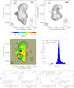 |
Fig. 8 Top: total intensity contours and polarization vectors of the radio sources in Abell 194. VLA image (left) at 1443 MHz (σI = 2 mJy/beam), smoothed with a FWHM Gaussian of 2.9′. SRT image (right) at 6600 MHz (σI = 1 mJy/beam), with a resolution of 2.9′. The radio contours are drawn at 3σI and the rest are spaced by a factor of 2. The lines give the orientation of the electric vector position angle (E-field) and are proportional in length to the fractional polarization. The vectors are only traced for those pixels where the total intensity signal is above 5σI, the error on the polarization angle is less than 10°, and the fractional polarization is above 3σFPOL. Middle left: RM image calculated using the images at 1443, 1465, 1515, 1630, and 6600 MHz, smoothed with a FWHM Gaussian of 2.9′. The color range is from −60 to 60 rad/m2. Contours refer to the total intensity image at 1443 MHz as in the top left panel. Middle right: histogram of the RM distribution. Bottom: plots of the position angle Ψ as a function of λ2 at four different source locations. |
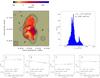 |
Fig. 9 Top left: burn law a in rad2/m4 calculated using the images at 1443, 1465, 1515, 1630, and 6600 MHz smoothed with a FWHM Gaussian of 2.9′. The image is derived from a fit of FPOL as a function of λ4 following the Eq. (5). The color range is from −500 to 1300 rad2/m4. Contours refer to the total intensity image at 1443 MHz. The radio contours are drawn at 3σI and the rest are spaced by a factor of 2. Top right: histogram of the Burn law a distribution. Bottom: plots of fractional polarization FPOL as a function of λ4 at four different source locations. |
In the top panels of Fig. 8 we compare the polarization image observed with the SRT at 6600 MHz (right) with that obtained with the VLA at 1443 MHz (left), smoothed with a FWHM Gaussian of 2.9′.
The fractional polarization at 1443 MHz is similar to that at 6600 MHz being ≃3–5% in 3C 40A and in the brightest part of the radio lobes of 3C 40B. The fractional polarization increases in the low surface brightness of the northern lobe of 3C 40B where it is ≃15%. The oldest low-brightness regions are visible both in total intensity and polarization at 1443 MHz but not at 6600 MHz because of the sharp high-frequency cutoff of the synchrotron spectrum. These structures, located east of 3C 40B and in the southern lobe of 3C 40B, show a fractional polarization as high as ≃20–50% at 1443 MHz (see Sect. 7).
By comparing the orientation of the polarization vectors at the different frequencies it is possible to note a rotation of the position angle. We interpret this as due to the Faraday rotation effect. The observed polarization angle Ψ of a synchrotron radio source is modified from its intrinsic value Ψ0 by the presence of a magneto-ionic Faraday screen between the source of polarized emission and the observer. In particular, the plane of polarization rotates according to 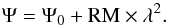 (3)The RM is related to the plasma thermal electron density, ne, and magnetic field along the LOS, B∥ of the magneto-ionic medium, by the equation
 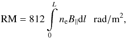 (4)where B∥ is measured in μG, ne in cm-3, and L is the depth of the screen in kpc.
Following Eq. (3), we obtained the RM image of Abell 194, by performing a fit pixel by pixel of the polarization angle images as a function of λ2 with the FARADAY software (Murgia et al. 2004). Given as input multifrequency images of Q and U, the software produces the RM, intrinsic polarization angle Ψ0, and corresponding error images. To improve the RM image, the algorithm can be iterated in several self-calibration cycles. In the first cycle only pixels with the highest signal-to-noise ratio are fitted. In the next cycles the algorithm uses the RM information in these high signal-to-noise pixels to solve the nπ ambiguity in adjacent pixels of lower signal-to-noise, following a similar method used in the PACERMAN algorithm by Dolag et al. (2005).
In the middle left panel of Fig. 8, we show the resulting RM image at an angular resolution of 2.9′. The values of RM range from −60 to 60 rad/m2 with the higher absolute values in the central region of the cluster in between the cores of 3C 40B and 3C 40A. We obtained this image by performing the λ2 fit of the polarization angle images at 1443, 1465, 1515, 1630, and 6600 MHz. The total intensity contours at 1443 MHz are overlaid on the RM image. The RM image was only derived in those pixels in which the following conditions were satisfied: the total intensity signal at 1443 MHz was above 3σI, the resulting RM fit error was lower than 5 rad/m2, and in at least four frequencies the error in the polarization angle was lower than 10°.
In the bottom panels of Fig. 8, we show a few plots of the position angle Ψ as a function of λ2 at different source locations. The plots show some pixels, located in different parts of the sources, with representative RM. Thanks to the SRT image, we can effectively observe that the data are generally quite well represented by a linear λ2 relation over a broad λ2 range, which supports the external Faraday screen hypothesis.
We can characterize the RM distribution in terms of a mean ⟨ RM ⟩ and root mean square σRM. In the middle right panel of Fig. 8, we show the histogram of the RM distribution. The mean and root mean square of the RM distribution are ⟨ RM ⟩ = 15.2 rad/m2 and σRM = 14.4 rad/m2, respectively. The mean fit error of the RM error image is ≃1.6 rad/m2. The dispersion σRM of the RM distribution is higher than the mean RM error. Therefore, the RM fluctuations observed in the image are significant and can give us information on the cluster magnetic field power spectrum.
For a partially resolved foreground with Faraday rotation in a short-wavelength limit, a depolarization of the signal due to the unresolved RM structures in the external screen can be approximated, to first order, with the Burn law (Burn 1966; see also Laing et al. 2008, for a more recent derivation), 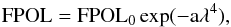 (5)where FPOL0 is the fractional polarization at λ = 0 and a = 2 | ∇RM | 2σ2 is related to the depolarization due to the RM gradient within the observing beam considered a circular Gaussian with FWHM = 2
 .
.
The effect of depolarization between two wavelengths, λ1 and λ2, is usually expressed in terms of the ratio of the degree of polarization DP = FPOL(λ2)/FPOL(λ1). The Burn law can provide depolarization information by considering the data at all frequencies simultaneously. However, the polarization behavior varies as the Burn law at short wavelengths and goes to a simple generic power-law form at long wavelengths (Tribble 1991).
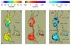 |
Fig. 10 Left: rotation measure image calculated with the images at 1443, 1630, 4535, and 4885 MHz smoothed with a FWHM Gaussian of 19′′. The color range is from −60 to 60 rad/m2. Contours refer to the total intensity image at 1443 MHz. Levels are 1 (3σI), 5, 30, and 100 mJy/beam. Middle: burn law a in rad2/m4 calculated with the same images used to derive the RM. The image is derived from a fit of FPOL as a function of λ4 following the Eq. (5). The color range is from −500 to 1300 rad2/m4. Right: intrinsic polarization (Ψ0 and FPOL0), obtained by extrapolating to λ = 0 both the RM (Eq. (3)) and the Burn law (Eq. (5)). |
Following Laing et al. (2008), in the top left panel of Fig. 9 we show the image of the Burn law exponent a derived from a fit to the data. We obtain this image by performing the λ4 fit of the fractional polarization FPOL images at 1443, 1465, 1515, 1630, and 6600 MHz, using at least four of these frequencies in each pixel. The values of a range from −500 to 1300 rad2/m4. The histogram of the Burn law a distribution is shown in the top right panel of Fig. 9. A large number of pixels have a ≃ 0 indicating no depolarization. Significant depolarization (a> 0) is found close to 3C 40A. Finally, a minority of pixels have a< 0. This may be due to the noise or the effect of Faraday rotation on a non-uniform distribution of intrinsic polarization (Laing et al. 2008). Indeed, repolarization of the signal is not unphysical and perfectly possible (e.g., Farnes et al. 2014; Lamee et al. 2016). Example plots of a as a function of λ4 are shown in the bottom panels of Fig. 9. The plots show the same pixels of Fig. 8. In these plots, the Burn law gives adequate fits in the frequency range and resolution of these observations.
We used the images presented in Fig. 8 and in Fig. 9 to investigate the variation of the magnetic field strength in the cluster volume. In addition, to measure the correlation length of the magnetic field fluctuations, we used the archival VLA observations to improve the RM resolution in the brightest parts of the sources.
6.2. Polarization data at 19′′ and 60′′ resolution
In the left panel of Fig. 10 we show the resulting RM image at an angular resolution of 19′′. In the middle panel of Fig. 10, we show the resulting Burn law image at the same angular resolution. We derived these images with VLA data at 1443, 1630, 4535, and 4885 MHz and by adopting the same strategy described in Sect. 6.1 for the lower resolution images. The noise levels of the images at a resolution of 19′′ are given in Table 5. Qualitatively, the brightest parts of the 3C 40A and 3C 40B sources show RM and Burn law images, which is in agreement with what we find at lower resolution. However, at this resolution the two sources are well separated and the RM structures can be investigated in finer detail. In particular, the RM distribution seen over the two radio galaxies is patchy, indicating a cluster magnetic field with turbulent structures on scales of a few kpc.
Relevant parameters of the total intensity and polarization images at a resolution of 19′′.
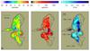 |
Fig. 11 Left: rotation measure image calculated with the images at 1443, 1465, 1515, and 1630 MHz smoothed with a FWHM Gaussian of 60′′. The color range is from −60 to 60 rad/m2. Contours refer to the total intensity image at 1443 MHz. Levels are 1.5 (3σI), 5, 30, and 100 mJy/beam. Middle: burn law a in rad2/m4 calculated with the same images used to derive the RM. The image is derived from a fit of FPOL as a function of λ4 following the Eq. (5). The color range is from −500 to 1300 rad2/m4. Right: intrinsic polarization (Ψ0 and FPOL0), obtained by extrapolating to λ = 0 both the RM (Eq. (3)) and the Burn law (Eq. (5)). |
In the left and middle panel of Fig. 11 we show the resulting RM and Burn law images at an angular resolution of 60′′. We derived these images via VLA data at 1443, 1465, 1515, and 1630 MHz and by adopting the same strategy described in Sect. 6.1. The noise level of the images at a resolution of 60′′ are given in Table 4. The RM image at 60′′ is consistent with that at 2.9′, although obtained in a narrower λ2 range.
Low polarization structures may potentially cause images with some artefacts. However, these effects are taken into account in the magnetic field modeling since simulations and data are filtered in the same way. The data at 19′′ and 60′′ are used to derive realistic models for the intrinsic properties of the radio galaxies. These models are used to produce synthetic polarization images at arbitrary frequencies and resolutions in our magnetic field modeling (see Sect. 7).
In the right panel of Fig. 10 we show the intrinsic polarization image at 19′′ of 3C 40A and 3C 40B. The intrinsic polarization (Ψ0 and FPOL0) was obtained by extrapolating to λ = 0 both the RM (Eq. (3)) and the Burn law (Eq. (5)). The image reveals regions of high fractional polarization. The panel shows some representative values of fractional polarization with the corresponding uncertainty. The southern lobe of 3C 40B shows an outer rim of high fractional polarization (≃50%) to the southeast. These polarization rims are commonly observed at the boundary of the lobes of both low (e.g., Capetti et al. 1993) and high (e.g., Perley & Carilli 1996) luminosity radio galaxies. The rim-like morphology of high fractional polarization is an expected feature that is usually interpreted as the compression of the lobes magnetic field along the contact discontinuity. The normal field components near the edge are suppressed and only tangential components survive giving rise to very high fractional polarization levels.
This image provides a description of the intrinsic polarization properties in the brightest part of the sources. However, we also need information in the fainter parts of the sources for modeling at large distances from the cluster center. In this case we obtained the information from the data at a resolution of 60′′. In the right panel of Fig. 11 we show the intrinsic polarization image at 60′′, derived by extrapolating to λ = 0 both the RM formula and the Burn law. The two images are in good agreement in the common parts. In addition, they complement the intrinsic polarization information in different sampling regions of the sources. The intrinsic (λ = 0) fractional polarization images shown in Figs. 10 and 11 confirm very low polarization levels in coincidence with the peak intensity in the southern lobe, which is in agreement with the small length measured for the fractional polarization vectors overimposed to the polarization image obtained with the SRT at 6600 MHz and shown in Fig. 2. Furthermore, the higher S/N ratio of the low resolution image reveals a few steep spectrum diffuse features not observable in Fig. 10. In particular, this reveals a trail to the east (see Sakelliou et al. 2008, for an interpretation), i.e., the northern part of the tail of 3C 40A, which overlaps in projection to the tip of the northern lobe of 3C 40B, and a tail extending from the southern lobe of 3C 40B. A common property of these features is that they are all highly polarized as indicated in the figure. These are likely very old and relaxed regions characterized by an ordered magnetic field. The combination of these two effects could explain the high fractional polarization observed.
Rotation measure results.
6.3. Polarization results summary
The SRT high-frequency observations are essential to determine the large-scale structure of the RM in Abell 194. While the angular size of the lobes shown in Fig. 10 are comparable with the largest angular scale detectable by the VLA in D configuration at C band (≃5′), the full angular extent of 3C 40 B is so large (≃20′) that the intrinsic structure of the U and Q parameters can be properly recovered only with single-dish observations. Indeed, the SRT observation at 6600 MHz is fundamental because it makes it possible to ensure that the polarization position angles follow the λ2 law over a broad range of wavelengths thus confirming the hypothesis that the RM originates in an external Faraday screen.
The observed RM fluctuations in Abell 194 appear to be similar to those observed for other sources in comparable environments, for example, NGC 6251, 3C 449, and NGC 383, (Perley et al. 1984; Feretti et al. 1999a; Laing et al. 2008), but are much smaller in amplitude than in rich galaxy clusters (e.g., Govoni et al. 2010).
We summarize the RM results obtained at the different resolutions in Table 6. The values of ⟨ RM ⟩ given in Table 6 include the contribution of the Galaxy. We determined the RM Galactic contribution with the results by Oppermann et al. (2015), mostly based on the catalog by Taylor et al. (2009), which contains the RM for 34 radio sources within a radius of 3 deg from the cluster center of Abell 194. Within this radius, the RM Galactic contribution results to be 8.7 ± 4.5 rad/m2. Therefore, half of the ⟨ RM ⟩ value measured in the Abell 194 sources is Galactic in origin.
In 3C 40B the two lobes show a similar RM and Burn law a; this is in contrast to what was found in 3C 31 (Laing et al. 2008), where asymmetry between the north and south sides is evident. While 3C 31 is inclined with respect the plane of the sky and the receding lobe is more rotated than the approaching lobe (Laing-Garrinton effect; Laing 1988; Garrinton et al. 1988), in Abell 194, our results seem to indicate that the two lobes of 3C 40B lay on the plane of the sky, and thus they are affected by a similar physical depth of the Faraday screen. It is also interesting to note that 3C 40A is located at a projected distance from the cluster center very similar to that of the southern lobe of 3C 40B, but 3C 40A is more depolarized than the southern lobe of 3C 40B. This behavior may be explained if 3C 40A is located at a deeper position along the line of sight than 3C 40B. Thus, passing across a longer path, the signal is subject to a higher depolarization owing to the higher RM. Other explanations may be connected to the presence of the X-ray cavity in the southern lobe of 3C 40B, which might reduce its depolarization with respect to 3C 40A.
The FPOL trend with λ4 and the polarization angle trend with λ2 would argue in favor of an RM produced by a foreground Faraday screen (Burn 1966; Laing 1984; Laing et al. 2008). In addition, the presence of a large X-ray cavity formed by the southern radio lobe arising from 3C 40B (Bogdán et al. 2011) supports the scenario in which the rotation of the polarization plane is likely to occur entirely in the intra-cluster medium, since the radio lobe is likely voided of thermal gas.
In a few cases (Guidetti et al. 2011) the RM morphologies tend to display peculiar anisotropic RM structures. These anisotropies appear highly ordered (“RM bands”) with iso-contours orthogonal to the axes of the radio lobes and are likely related to the interaction between the sources and their surroundings. The RM images of Abell 194 show patchy patterns without any obvious preferred direction, in agreement with many of the published RM images. Therefore, in Abell 194, the standard picture that the Faraday effect is due to the turbulent intra-cluster medium and not affected by the presence of the radio source itself is self-consistent. These above considerations suggest that the effect of the external Faraday screen is dominant over the internal Faraday rotation, if it exists.
As shown in optical and X-ray analyses (see Sects. 4.2 and 4.3), Abell 194 is not undergoing a major merger event. Rather it is likely that is it accreting several smaller clumps. Under these conditions, we do not expect injection of turbulence on cluster-wide scales in the intra-cluster medium. However, we may expect injection of turbulence on scales of a few hundred kpc due to the accretion flows of small groups of galaxies, the motion of galaxy cluster members, and the expansion of radio lobes. This turbulent energy cascades on smaller scales, is dissipated, and finally heats the intra-cluster medium. The footprint of this cascade could be observable on the intra-cluster magnetic field structure through the RM images. In this case, the patchy structure characterizing the RM images in Figs. 8, 10, and 11 can be interpreted as a signature of the turbulent intra-cluster magnetic field and the values of the σRM and ⟨ RM ⟩ can be used to constrain the strength and structure of the magnetic field.
Parameters of the magnetic field model.
7. Intra-cluster magnetic field characterization
We constrained the magnetic field power spectrum in Abell 194 using the polarization information (RM and fractional polarization) derived for the radio galaxies 3C 40A and 3C 40B. A realistic description of the cluster magnetic fields must simultaneously provide a reasonable representation of the following observables:
-
the RM structure function defined by
![Mathematical equation: \begin{equation} S(\Delta x, \Delta y)=\langle [RM(x,y)-RM(x+\Delta x,y+\Delta y)]^2\rangle_{(x,y)}, \end{equation}](/articles/aa/full_html/2017/07/aa30349-16/aa30349-16-eq200.png) (6)where = ⟨ ⟩ (x,y) indicates that the average is taken over all the positions (x,y) in the RM image. The structure function S(Δr) was then computed by azimuthally averaging S(Δx,Δy) over annuli of increasing separation
(6)where = ⟨ ⟩ (x,y) indicates that the average is taken over all the positions (x,y) in the RM image. The structure function S(Δr) was then computed by azimuthally averaging S(Δx,Δy) over annuli of increasing separation  ;
; -
the Burn law (see Eq. (5)); and
-
the trends of σRM and ⟨ RM ⟩ against the distance from the cluster center.
The RM structure function and the Burn law are better investigated with the data at higher resolution (19′′), while the trends of σRM and ⟨ RM ⟩ with the distance from the cluster center are better described by the data at lower resolution (2.9′).
Our modeling is based on the assumption that the Faraday rotation occurs entirely in the intra-cluster medium. In particular, we supposed that there is no internal Faraday rotation inside the radio lobes.
To interpret the RM and the fractional polarization data, we need a model for the spatial distribution of the thermal electron density and the intra-cluster magnetic field.
For the thermal electrons density profile, we assumed the β-model derived in Sect. 4.3 with rc = 248.4 kpc, β = 0.67, and n0 = 6.9 × 10⁻⁴ cm-3.
For the power spectrum of the intra-cluster magnetic field fluctuations, we adopted a power law with index n of the form  (7)in the wave number range from kmin = 2π/ Λmax to kmax = 2π/ Λmin.
Moreover, we supposed that the power spectrum normalization varies with the distance from the cluster center such that the average magnetic field strength at a given radius scales as a function of the thermal gas density according to ![Mathematical equation: \begin{equation} \langle B(r)\rangle=\langle B_{\rm 0}\rangle\left[\frac{n_{\rm e}(r)}{n_{\rm 0}}\right]^{\rm \eta}, \label{eta} \end{equation}](/articles/aa/full_html/2017/07/aa30349-16/aa30349-16-eq213.png) (8)where ⟨ B0 ⟩ is the average magnetic field strength at the center of the cluster3 and ne(r) is the thermal electron gas density radial profile. The magnetic field fluctuations are considered isotropic on scales Λ ≫ Λmax, i.e., the fluctuations phases are completely random in the Fourier space.
(8)where ⟨ B0 ⟩ is the average magnetic field strength at the center of the cluster3 and ne(r) is the thermal electron gas density radial profile. The magnetic field fluctuations are considered isotropic on scales Λ ≫ Λmax, i.e., the fluctuations phases are completely random in the Fourier space.
Overall, our magnetic field model depends on the following five parameters listed in Table 7:
-
(i)
the strength at the cluster center⟨ B0 ⟩;
-
(ii)
the radial index η;
-
(iii)
the power spectrum index n;
-
(iv)
the minimum scales of fluctuation Λmin;
-
(v)
the maximum scales of fluctuation Λmax.
As pointed out in Murgia et al. (2004), there are a number of degeneracies between these parameters. In particular, the most relevant to us are the degeneracy between ⟨ B0 ⟩ and η, and between Λmin, Λmax, and n.
Fitting all of these five parameters simultaneously would be the best way to proceed but this is not feasible because of computational burdens. The aim of this work is to constrain the magnetic field radial profile, therefore we proceeded in two steps. First, we performed two-dimensional simulations to derive the magnetic field shape of the power spectrum. Second, we performed three-dimensional simulations varying the values of ⟨ B0 ⟩ and η and deriving the magnetic field profile that best reproduces the RM observations.
We focused our analysis on ⟨ B0 ⟩, η, and Λmax. In our modeling, Λmax should represent the injection scale of turbulent energy. Since Abell 194 is a rather relaxed cluster, we expect a Λmax to be a hundred kpc or less. The turbulent energy cascades down to smaller and smaller scales until it is dissipated. Determining the slope of the magnetic field power spectrum and the outer scale of the magnetic field fluctuations is not trivial because of the degeneracy between these parameters (see, e.g., Murgia et al. 2004; Bonafede et al. 2010). To reduce the number of free model parameters, on the basis of the Kolmogorov theory for a turbulent medium, we fixed the slope of the power-law power spectrum to n = 11 / 3. In addition, we fixed Λmin = 1 kpc. A different Λmin has a negligible impact on these simulation results since, for a Kolmogorov spectral index, most of the magnetic field power is on larger scales and our observations do not resolve sub-kpc structures.
In particular, using the 19′′ resolution data set, we performed a two-dimensional analysis to constrain the maximum scale of the magnetic field fluctuations Λmax and, using the 2.9′ resolution data set, we performed three-dimensional numerical simulations to constrain the strength of the magnetic field and its scaling with the gas density. In both cases, we used the FARADAY code (Murgia et al. 2004) to produce simulated RM and fractional polarization images and to compare them with the observed images. The simulated images were produced by integrating numerically the gas density and magnetic field product along the LOS. We considered the sources 3C 40 A and 3C 40 B lying in the plane of the sky (not inclined) and the limits of the integrals were [0,1 Mpc], i.e., with the sources located at the cluster center. In the simulated RM images we took into account the Galactic RM contribution, which is supposed to be uniform over the radio sources 3C 40 A and 3C 40 B.
Owing to the heavy window function imposed by the limited projected size of the radio galaxies with respect to the size of the cluster, for a proper comparison with observations, the simulated fractional polarization and RM images are filtered like the observations before comparing them to data. The two-dimensional and three-dimensional simulations are filtered following these steps:
-
(1)
We created a source model at 19′′ (for the two-dimensional analysis) and at 60′′ (for the three-dimensional analysis) by considering the CLEAN components (CC model) of the images at 1443 MHz. For each observing frequency, we then derived the expected total intensity images I(ν) obtained by associating at each CLEAN component the corresponding flux density calculated by assuming a JP model with αinj = 0.5 and νb taken from the observed break frequency image (see Fig. 7 and Sect. 5).
-
(2)
We used the images in the right panels of Figs. 10 and 11, which were obtained by extrapolating the Burn law at λ = 0, as a model of intrinsic fractional polarization FPOL0, thus removing the wavelength-dependent depolarization due to the foreground Faraday screen. In this way, FPOL0 accounts for the intrinsic disorder of the magnetic field inside the radio source, which may vary in general from point to point. For each observing frequency, we then derived the expected “full-resolution” fractional polarization FPOL(ν) obtained by associating at each CLEAN component the intrinsic fractional polarization corrected for the aging effect derived from the break frequency image shown in Fig. 7 as follows:
 (9)Murgia et al. (2016) pointed out that, as the synchrotron plasma ages, the theoretical fractional polarization4 approaches 100% for ν ≫ νb. The canonical value FPOLtheor = (3p + 3) / (3p + 7), which is valid for a power-law emission spectrum, is obtained in the limit ν ≪ νb.
 -
(3)
For the intrinsic polarization angle Ψ0, we assigned at each CLEAN component the values taken from the images in the right panels of Figs. 10 and 11, obtained by extrapolating the Ψ at λ = 0.
-
(4)
Using I(ν), FPOL(ν), and Ψ0, we produced the expected Q(ν) and U(ν) images corresponding to the simulated RM, obtained by employing Eq. (3).
-
(5)
We added a Gaussian noise such as that of the observations to the I(ν), Q(ν), and U(ν) images and we smoothed them with the FWHM beam of the observations used in the two-dimensional and three-dimensional analysis (19′′ or 2.9′). In this way we have taken into account the beam depolarization of the polarized signal.
-
(6)
Finally, we derived the fractional polarization images FPOL(ν) = P(ν)/I(ν) from synthetic I(ν), Q(ν), and U(ν) images and we produced the synthetic RM image by fitting pixel by pixel the polarization angle images Ψ(ν) versus the squared wavelength using exactly the same algorithm and strategy described in Sect. 6 as if they were actual observations.
Examples of observed and synthetic images used in our analysis are shown in Fig. 12.
Following Vacca et al. (2012), we compared the synthetic images and data using the Bayesian inference, whose use was first introduced in the RM analysis by Enßlin & Vogt (2003).
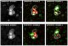 |
Fig. 12 Example of observed (top panels) and synthetic (bottom panels) Stokes parameters for the SRT observations at 6600 MHz and 2.9′resolution. |
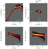 |
Fig. 13 Bayesian two-dimensional analysis of the RM structure function S(Δr) and depolarization ratio FPOL/FPOL0(λ4). Top right panel: image of the posterior distribution of the model parameters along with one-dimensional marginalizations. Top left panel: dots represent the observed S(Δr) (error bars are comparable to the size of the symbols). The fan plot represents the population of synthetic RM structure functions from the posterior distribution. Bottom left panel: depolarization ratio as a function of λ4 for the southern lobe of 3C 40B. The dots represent the observed data while the fan plot represents the population of synthetic depolarization ratio extracted from the posterior distribution of model parameters. Bottom right panel: depolarization ratio as a function of λ4 for the northern lobe of 3C 40B. |
7.1. Bayesian inference
Because of the random nature of the intra-cluster magnetic field fluctuations, the RM and fractional polarization images we observe are just one possible realization of the data. Thus, rather than try to determine the particular set of power spectrum parameters, θ, that best reproduces the given realization of the data, it is perhaps more meaningful to search for the distribution of model parameters that maximizes the probability of the model given the data. The Bayesian inference offers a natural theoretical framework for this approach.
The Bayesian rule relates our prior information on the distribution P(θ) of model parameters θ to their posterior probability distribution P(θ | D) after the data D have been acquired, i.e., 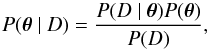 (10)where P(D | θ) is the likelihood function, while P(D) is called the evidence. The evidence acts as a normalizing constant and represents the integral of the likelihood function weighted by the prior over all the parameters space
 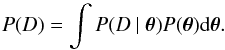 (11)The most probable configuration for the model parameters is obtained from the posterior distribution given by the product of the likelihood function with the prior probability. We used a Markov chain Monte Carlo (MCMC) method to extract samples from the posterior probability distribution. In particular, we implemented the Metropolis−Hastings algorithm, which is capable of generating a sample of the posterior distribution without the need to calculate the evidence explicitly, which is often extremely difficult to compute since it would require exploring the entire parameters space. The MCMC is started from a random initial position θ0 and the algorithm is run for many iterations by selecting new states according to a transitional kernel, Q(θ,θ′), between the actual, θ, and the proposed position, θ′. The proposed position is accepted with probability
 ![Mathematical equation: \begin{equation} h=\min \left[1, \frac{P(D~\vert~ \vec\theta ^{\rm \prime}) P( \vec\theta^{\rm \prime}) Q( \vec\theta ^{\rm \prime}, \vec\theta ) } { P(D~\vert~ \vec\theta) P( \vec\theta) Q( \vec\theta , \vec\theta ^{\rm \prime}) } \right]\cdot \end{equation}](/articles/aa/full_html/2017/07/aa30349-16/aa30349-16-eq242.png) (12)We chose for Q a multivariate Gaussian kernel. The MCMC starts with a number of “burn-in” steps during which, according to common practice, the standard deviation of the transitional kernel is adjusted so that the average acceptance rate stays in the range 25%−50%. After the burn-in period, the random walk forgets its initial state and the chain reaches an equilibrium distribution. The burn-in steps are discarded and the remaining set of accepted values of θ is a representative sample of the posterior distribution that can be used to compute the final statistics on the model parameters.
(12)We chose for Q a multivariate Gaussian kernel. The MCMC starts with a number of “burn-in” steps during which, according to common practice, the standard deviation of the transitional kernel is adjusted so that the average acceptance rate stays in the range 25%−50%. After the burn-in period, the random walk forgets its initial state and the chain reaches an equilibrium distribution. The burn-in steps are discarded and the remaining set of accepted values of θ is a representative sample of the posterior distribution that can be used to compute the final statistics on the model parameters.
7.2. Two-dimensional simulations
The polarization images at a resolution of 19′′ give a detailed view of the magnetic field fluctuations toward the brightest parts of the radio sources. For this reason, we performed a two-dimensional analysis of these data to constrain the maximum scale of the magnetic field fluctuations, Λmax, by fixing n = 11 / 3 and Λmin = 1 kpc.
Within the power-law scaling regime (Enßlin & Vogt 2003), the two-dimensional analysis relies on the proportionality between the magnetic field and the RM power spectra. On the basis of this proportionality, the slope n of the two-dimensional RM power spectrum is the same as the three-dimensional magnetic field power spectrum, i.e., 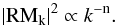 (13)We simulated RM images with a given power spectrum in a two-dimensional grid. The simulations start in the Fourier space, where the amplitudes of the RM components are selected according to Eq. (13), while the phases are completely random. The RM image in the real space is obtained by a fast Fourier transform (FFT) inversion. We have taken into account the dependence of the RM on the radial decrease of the thermal gas density and of the intra-cluster magnetic field by applying a tapering to the RM image
  (14)for which we fixed the parameters of the β-model (Sect. 4.3) and we assumed in first approximation η = 1.
As a compromise between computational speed and spatial dynamical range, we adopted a computational grid of 1024 × 1024 pixels with a pixel size of 0.5 kpc. This grid allowed us to explore RM fluctuations on scales as small as Λmin = 1 kpc, which is smaller than the linear size of the 19′′ beam of the observations FWHM ≃ 6.8 kpc. At the same time, we were able to investigate fluctuations as large as Λmax = 512 kpc, i.e., comparable to the linear size of the radio galaxy 3C 40B in Abell 194.
To the aim of the Bayesian inference outlined in Sect. 7.1, we adopted a likelihood of the form ![Mathematical equation: \begin{equation} P(D~\vert~ \vec\theta)=\prod_{i} \frac{1}{\sigma_{\rm synth}(i)\sqrt{2\pi}} \exp \left[-\frac{1}{2}\frac{\left[D_{\rm obs}(i)-D_{\rm synth}(i)\right]^2}{\sigma_{\rm synth}(i)^2}\right], \label{boo} \end{equation}](/articles/aa/full_html/2017/07/aa30349-16/aa30349-16-eq249.png) (15)where the observed data Dobs are compared to the synthetic data Dsynth. The synthetic data are obtained by filtering simulations as the observations (as described in Sect. 7). The scatter σsynth includes both the simulated noise measurements, σnoise, and the intrinsic statistical scatter of the synthetic data, σDsynth, due to the random nature of the intra-cluster magnetic fields:
(15)where the observed data Dobs are compared to the synthetic data Dsynth. The synthetic data are obtained by filtering simulations as the observations (as described in Sect. 7). The scatter σsynth includes both the simulated noise measurements, σnoise, and the intrinsic statistical scatter of the synthetic data, σDsynth, due to the random nature of the intra-cluster magnetic fields:  . At each step of the MCMC, for a given combination of the free parameters θ, we performed five simulations with different realizations of the fluctuations phases, and we evaluated the dispersion σsynth.
In our two-dimensional analysis, the data D (observed and synthetic) are represented by the azimuthally averaged RM structure function S(Δr) and by the depolarization ratio FPOL/FPOL0(λ4). The posterior distribution for a given set of model parameters is computed by considering the joint likelihood of the RM structure function and the depolarization ratio all together. We applied the Bayesian method by choosing priors uniform in logarithmic scale for the two free parameters: normalization of the magnetic field power spectrum norm and minimum wave number kmin.
In the top right panel of Fig. 13 we show the image of the posterior distribution for the two free parameters norm and kmin. In addition, one-dimensional marginalizations are shown as histograms along each axis of the image. The one-dimensional marginalizations represent the projected density of samples in the MCMC, which is proportional to the posterior probability of that particular couple of model parameters.
To provide a visual comparison between synthetic and observed data we present the fan plots of the structure function and depolarization ratio.
In the top left panel of Fig. 13 the dots represent the observed RM structure function S(Δr) calculated using the RM image of Fig. 10. The observed RM structure function S(Δr) is shown together with the population of synthetic structure functions extracted from the posterior distribution. Brighter pixels in the fan plot occur where many different synthetic structure functions overlap each other. Thus, the fan plot gives a visual indication of the marginalized posterior probability of the synthetic data at a given separation. Overall, the fan plot shows that the Kolmogorov power spectrum is able to reproduce the shape of the observed RM structure function, including the large-scale oscillation observed before the turnover at Δr> 100 kpc. The turnover is likely caused by undersampling of the large separations imposed by the window function due to the silhouette of the radio sources combined with the effect of the tapering imposed by the dimming of the gas density and magnetic field strength at increasing distances from the cluster center. On small separations, Δr< 6.8 kpc, the slope of the structure function is affected by the observing beam. It is worth mentioning that all these effects are fully taken into account when simulating the synthetic I, Q, and U images.
In the bottom panels of Fig. 13 the dots represent FPOL/FPOL0 as a function of λ4 calculated in the southern (left panel) and in the northern (right panel) lobe of 3C 40B, respectively. The southern lobe, is slightly more depolarized than the northern lobe. The statistics of the fractional polarization were calculated considering only the pixels in which FPOL > 3σFPOL. The observed depolarization ratio as a function of λ4 is shown, together with the fan plots of the synthetic depolarization. In general, the Kolmogorov power spectrum is able to reproduce the observed depolarization, as shown by the fan plots.
To summarize, the combined two-dimensional analysis of RM structure function and fractional polarization allowed us to constrain the maximum scales on the magnetic field fluctuations to Λmax = (64 ± 24) kpc, where the given error represents the dispersion of the one-dimensional marginalizations.
The magnetic field autocorrelation length is calculated according to  (16)where the wave number k = 2π/ Λ (Enßlin & Vogt 2003). We obtained ΛB = (20 ± 8) kpc.
In the next step we fix this value and we constrain the strength of the magnetic field and its scaling with the gas density with the aid of three-dimensional simulations.
7.3. Three-dimensional simulations
The data at a resolution of 2.9′ are best suited to derive RM information up to a large distance from the cluster center. Therefore, we used these data to constrain the strength of the magnetic field and its scaling with the gas density using three-dimensional simulations.
We constructed three-dimensional models of the intra-cluster magnetic field by following the numerical approach described in Murgia et al. (2004). The simulations begin in Fourier space by extracting the amplitude of the magnetic field potential vector,  , from a Rayleigh distribution whose standard deviation varies with the wave number according to | Ak | 2 ∝ k− n−2. The phase of the potential vector fluctuations is taken to be completely random. The magnetic field is formed in Fourier space via the cross product
  . This ensures that the magnetic field is effectively divergence free. We then perform a three-dimensional FFT inversion to produce the magnetic field in the real space domain. The field is then Gaussian and isotropic in the sense that there is no privileged direction in space for the magnetic field fluctuations. The power spectrum normalization is set such that the average magnetic field strength scales as a function of the thermal gas density according to Eq. (8). The gas density profile is described by the β-model in Eq. (1), modified, as for A2199 by Vacca et al. (2012), to take into account of the presence of the X-ray cavity detected in correspondence of the south lobe of 3C 40B.
We simulated the random magnetic field using a cubic grid of 10243 cells with a cell size of 0.5 kpc/cell. The simulated magnetic field is periodic at the boundaries and thus the computational grid is replicated to cover a larger cluster volume.
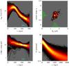 |
Fig. 14 Bayesian three-dimensional analysis of the σRM and ⟨ RM ⟩ as a function of the distance from the cluster center. Top right panel: image of the posterior distribution of the model parameters along with one-dimensional marginalizations. Top left panel: dots represent the observed σRM profile as a function of the distance from the cluster center while the fan plot represents the population of synthetic σRM profile extracted from the posterior distribution of model parameters. Bottom left panel: dots represent the observed ⟨ RM ⟩ profile as a function of the distance from the cluster center while the fan plot represents the population of synthetic ⟨ RM ⟩ profile extracted from the posterior distribution of model parameters. The Galactic foreground of 8.7 rad/m2 (Oppermann et al. 2015) is indicated with a dashed line. Bottom right panel: trend of the mean magnetic field with the distance from the cluster center. |
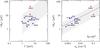 |
Fig. 15 Right panel: central magnetic field strength ⟨ B0 ⟩ vs. the mean cluster temperature. Red dots indicate cooling core clusters. Left panel: ⟨ B0 ⟩ vs. the central electron density n0. Red dots indicate cooling core clusters. Dashed line indicates the scaling obtained by a linear fit of the log-log relationship: ⟨ B0 ⟩∝ |
The simulated RM images were obtained by numerically integrating the magnetic field and the gas density product along the line of sight, accordingly to Eq. (4). In the case of Abell 194, the integration was performed from the cluster center up to 1 Mpc along the line of sight. As for the two-dimensional simulations, the simulated RM images were filtered like the observations. Finally, we used the Bayesian approach to find the posterior distribution for ⟨ B0 ⟩ and η. We derived the observed profiles of σRM and ⟨ RM ⟩ as a function of the distance from the cluster center by calculating the statistics in five concentric annuli of 2.9′ in size. The annuli are centered at the position of the X-ray centroid (see Sect. 4.3).
The slope n = 11 / 3 and the scales Λmin = 1 kpc and Λmax = 64 kpc were kept fixed at the values found in the two-dimensional analysis.
We applied the Bayesian method by choosing a uniform prior for the distribution of η and a prior uniform in logarithmic scale for the distribution of ⟨ B0 ⟩. At each step of the MCMC we simulated the synthetic I, Q, and U images of 3C 40A and 3C 40B and we derived the synthetic RM image following the same procedure as for the two-dimensional analysis. Using Eq. (15), we evaluated the likelihood of the σRM and ⟨ RM ⟩ profiles by means of ten different random configurations for the magnetic field phases to calculate the model scatter σDsynth.
The result of the Bayesian analysis is shown in Fig. 14. In the top right panel of Fig. 14, we present the image of the posterior distribution of model parameters along with the one-dimensional marginalizations represented as histograms.
In the top left panel of Fig. 14 we show the observed σRM profile along with the fan plot of the synthetic profiles from the posterior. The dispersion of the RM increases toward the cluster center as expected due to the higher density and magnetic field strength. The drop at the cluster center is likely caused by the undersampling of the RM statistics as a result of the smaller size of the central annulus with respect to the external annuli. In the bottom left panel of Fig. 14 we show the observed ⟨ RM ⟩ profile along with the fan plot of the synthetic RM profiles extracted from the posterior distribution. In this plot it is evident that the cluster shows an enhancement of the ⟨ RM ⟩ signal with respect to the Galactic foreground of 8.7 rad/m2 (Oppermann et al. 2015). Finally, in the bottom right panel of Fig. 14 we show the trend of the mean magnetic field with the distance from the cluster center.
The degeneracy between the central magnetic field strength and radial index is evident in the posterior distribution of model parameters: the higher ⟨ B0 ⟩ the higher η. However, we were able to constrain the central magnetic field strength to ⟨ B0 ⟩ = (1.5 ± 0.2) μG and the radial index to η = (1.1 ± 0.2). The average magnetic field over a volume of 1 Mpc3 is as low as ⟨ B ⟩ ≃ 0.3 μG. This result is obtained by fixing the slope of the magnetic field power spectrum to the Kolmogorov index. However, the central magnetic field strength depends on the square root of the field correlation length ΛB (see Eq. (16)). The field correlation length in turn depends on a combination of the power spectrum slope and Λmax and these two parameters are degenerate: a flatter slope for instance leads to a larger Λmax so that ΛB is preserved. Therefore, a different choice of the power spectrum slope n should have a second-order effect on the estimated central magnetic field strength. Nevertheless, as a further check, we repeated the two-dimensional Bayesian analysis (not shown) by freeing all the power spectrum parameters: normalization, Λmin, Λmax, and n. The larger dimensionality implies larger uncertainties owing to the computational burden needed to fully explore the parameters space. The maximum posterior probability is found for a slope n ≃ 3.6 ± 1.6, which is in agreement to within the large uncertainty with the Kolmogorov slope n = 11 / 3.
To our knowledge, the central magnetic field we determined in Abell 194 is the weakest ever found using RM data in galaxy clusters. However, Abell 194 is a poor galaxy cluster with no evidence of cool core.
It is interesting to compare the intra-cluster magnetic field of Abell 194 to that of other galaxy clusters for which a similar estimate is present in the literature. These are listed in Table 8.
Cluster magnetic field values taken from the literature.
In the left panel of Fig. 15 we show a plot of the central magnetic field strength ⟨ B0 ⟩ versus the mean cluster temperature, while in the right panel of Fig. 15 we show a plot of ⟨ B0 ⟩ versus the central electron density n0.
Although the cluster sample is still rather small, and thus all the following considerations should be taken with care, we note that there is a hint of a positive trend between ⟨ B0 ⟩ and n0 measured among different clusters. On the other hand, no correlation seems to be present between the central magnetic field and the mean cluster temperature, which is in agreement with what found by Govoni et al. (2010) in a statistical analysis of a sample of RM in rich galaxy clusters.
There are three merging clusters in the sample: Coma, A2255, and A119. They all have quite similar central magnetic field strengths even though Coma and A2255 host a giant radio halo while A119 is radio quiet. We confirm that cool core clusters, such as Hydra and A2199, tend to have higher central magnetic fields. In general, fainter central magnetic fields seem to be present in less dense galaxy clusters. Actually, this result is corroborated by the low central magnetic field found in this work for the poor galaxy cluster Abell 194. The scaling obtained by a linear fit of the log-log relationship is ⟨ B0 ⟩∝ . This result is in line with the theoretical prediction by Kunz et al. (2011), who assume that parallel viscous heating due to turbulent dissipation balances radiative cooling at all radii inside the cluster core. Kunz et al. (2011) found in the bremsstrahlung regime (that is T ≳ 1 keV)
  (17)where T is the temperature, while ξ is expected to range between 0.5 and 1 in a turbulent plasma. Following this formula, the expected magnetic field at the center of Abell 194 is 1.05ξ− 1 / 2μG. Although the central magnetic field found in our analysis is in remarkable agreement with the value obtained from Eq. (17), we found a magnetic field that scales with density as η = 1.1 ± 0.2, while according to Eq. (17), we should expect η = 0.5. However, we did not include in our analysis a possible scaling of B with the cluster temperature. If the intra-cluster medium is not isothermal, it is possible to bring the magnetic field radial profile found in our analysis in agreement with that in Eq. (17) supposing a temperature profile in Abell 194 as steep as T ∝ r-1.4 at large radii (r> 0.2R180). The temperature profile for Abell 194 is not known at large radii, but the required temperature profile is much steeper than the typical temperature decreases found in galaxy clusters, which are T ∝ r− μ with μ between 0.2 and 0.5 (e.g., Leccardi & Molendi 2008).
In Fig. 15, we plot the expected range of magnetic field strengths obtained with Eq. (17). In the right panel, the upper bound corresponds to ξ = 0.5 and T = 10 keV, while the lower bound corresponds to ξ = 1 and T = 1 keV. In the left panel, the upper bound corresponds to ξ = 0.5 and n0 = 5 × 10⁻⁴ cm-3, while the lower bound corresponds to ξ = 1 and n0 = 0.15 cm-3. Indeed for some reason it seems that the model by Kunz et al. (2011) seems to reproduce the scaling between central magnetic field and gas density among different galaxy clusters even if in the case of Abell 194 the observed magnetic field scaling with radius is significantly steeper than what they predict.
8. Summary and conclusions
In the context of the SRT early science program SMOG (SRT Multifrequency Observations of Galaxy clusters), we have presented a spectral-polarimetric study of the poor galaxy cluster Abell 194. We analyzed total intensity and polarization images of the extended radio galaxies 3C 40A and 3C 40B located close to the cluster center. By complementing the SRT observations with radio data at higher resolution and at different frequencies, but also with data in optical and X-ray bands, we aimed at inferring the dynamical state of the cluster, the radiative age of the radio galaxies, and the intra-cluster magnetic field power spectrum. The SRT data were used in combination with archival Very Large Array observations at lower frequencies to derive both spectral aging and RM images of 3C 40A and 3C 40B. The break frequency image and the cluster electron density profile inferred from ROSAT and Chandra observations are used in combination with the RM data to constrain the intra-cluster magnetic field power spectrum. Following Murgia et al. (2004), we simulated Gaussian random two-dimensional and three-dimensional magnetic field models with different power-law power spectra, and we compared the observed data and synthetic images with a Bayesian approach (Vogt & Enßlin 2005; Vacca et al. 2012) to constrain the strength and structure of the magnetic field associated with the intra-cluster medium. Our results can be summarized as follows:
-
To investigate the dynamical state of Abell 194and to obtain new additional insights into the cluster structure, weanalyzed the redshifts of 1893 galaxies from the literature,resulting in a sample of 143 fiducial cluster members. The pictureresulting from new and previous results agrees in thatAbell 194 does not show any trace of a major andrecent cluster merger, but rather agrees with a scenario ofaccretion of small groups, mainly along the NE−SW axis.
-
The measured break frequency in the radio spectra decreases systematically along the lobes of 3C 40B down to a minimum of 850 ± 120 MHz. If we assume that the magnetic field intrinsic to the source 3C 40B is in equipartition, the lifetimes of radiating electrons result to be 157 ± 11 Myr, in agreement with the spectral age estimate calculated by Sakelliou et al. (2008). Furthermore, the radiative age of 3C 40 B is consistent with that found in the literature for other sources of similar size and radio power (Parma et al. 1999).
-
Linearly polarized emission is clearly detected for both sources and the resulting polarization angle images are used to produce detailed RM images at different angular resolutions (2.9′, 60′′, and 19′′). The RM images of Abell 194 show patchy patterns without any obvious preferred direction, in agreement with the standard picture that the Faraday effect is due to the turbulent intra-cluster medium.
Table 9Results of the intra-cluster magnetic field power spectrum in Abell 194.
-
The results of the magnetic field power spectrum in Abell 194 are reported in Table 9. By assuming a Kolmogorov magnetic field power-law power spectrum (slope n = 11 / 3) with a minimum scale of fluctuations Λmin = 1 kpc, we find that the RM data in Abell 194 are well described by a magnetic field with a maximum scale of fluctuations of Λmax = (64 ± 24) kpc. The corresponding magnetic field autocorrelation length is ΛB = (20 ± 8) kpc. We find a magnetic field strength of ⟨ B0 ⟩ = (1.5 ± 0.2) μG at the cluster center. To our knowledge, the central magnetic field we determined in Abell 194 is the weakest ever found using RM data in galaxy clusters. However, Abell 194 is a poor galaxy cluster with no evidence of cool core. Our results also indicate a magnetic field strength that scales as the thermal gas density. In particular, the field decreases with the radius following the gas density to the power of η = (1.1 ± 0.2).
-
We compared the intra-cluster magnetic field determined for Abell 194 to that of a small sample of galaxy clusters for which a similar estimate was available in the literature. No correlation seems to be present between the mean central magnetic field and the cluster temperature. On the other hand, there is a hint of a trend between the central electron densities and magnetic field strengths among different clusters: ⟨ B0 ⟩∝
.
The radius Rδ is the radius of a sphere with mass overdensity δ times the critical density at the redshift of the galaxy system.
Since the simulated magnetic field components follow a Gaussian distribution, the total magnetic field is distributed according to a Maxwellian. In this work we quote the average magnetic field strength, which is related to the rms magnetic field strength through  .
.
The theoretical fractional polarization level FPOLtheor(ν/νb), expected for αinj = 0.5, is shown in Fig. 15 of Murgia et al. (2016).
Acknowledgments
We thank the anonymous referee for the useful comments that helped to improve the paper. The Sardinia Radio Telescope (SRT; Bolli et al. 2015; Prandoni et al. 2017) is funded by the Department of University and Research (MIUR), Italian Space Agency (ASI), and the Autonomous Region of Sardinia (RAS) and is operated as National Facility by the National Institute for Astrophysics (INAF). The development of the SARDARA backend has been funded by the Autonomous Region of Sardinia (RAS) using resources from the Regional Law 7/2007 “Promotion of the scientific research and technological innovation in Sardinia” in the context of the research project CRP-49231 (year 2011, PI Possenti): “High resolution sampling of the Universe in the radio band: an unprecedented instrument to understand the fundamental laws of the nature”. This research was partially supported by PRIN-INAF 2014. The National Radio Astronomy Observatory (NRAO) is a facility of the National Science Foundation, operated under cooperative agreement by Associated Universities, Inc. This research made use of the NASA/IPAC Extragalactic Database (NED), which is operated by the Jet Propulsion Laboratory, California Institute of Technology, under contract with the National Aeronautics and Space Administration. F. Loi gratefully acknowledges Sardinia Regional Government for the financial support of her Ph.D. scholarship (P.O.R. Sardegna F.S.E. Operational Programme of the Autonomous Region of Sardinia, European Social Fund 2007–2013 – Axis IV Human Resources, Objective l.3, Line of Activity l.3.1.). Basic research in radio astronomy at the Naval Research Laboratory is funded by 6.1 Base funding. This research was supported by the DFG Forschengruppe 1254 “Magnetisation of Interstellar and Intergalactic Media: the Prospects of Low-Frequency Radio Observations”. F. Vazza acknowledges funding from the European Union’s Horizon 2020 research and innovation program under the Marie-Sklodowska-Curie grant agreement No. 664931.
References
- Abell, G. O., Corwin, H. G. Jr., & Olowin, R. P. 1989, ApJS, 70, 1 [NASA ADS] [CrossRef] [EDP Sciences] [Google Scholar]
- Anders, E., & Grevesse, N. 1989, Geochim. Cosmochim. Acta, 53, 197 [Google Scholar]
- Arnaud, K. A. 1996, in Astronomical Data Analysis Software and Systems V, ASP Conf. Ser. 101, 5, 17 [NASA ADS] [Google Scholar]
- Barton, E. J., De Carvalho, R. R., & Geller, M. J. 1998, AJ, 116, 1573 [NASA ADS] [CrossRef] [Google Scholar]
- Beers, T. C., Flynn, K., & Gebhardt, K. 1990, AJ, 100, 32 [NASA ADS] [CrossRef] [Google Scholar]
- Bird, C. M., & Beers, T. C. 1993, AJ, 105, 1596 [NASA ADS] [CrossRef] [Google Scholar]
- Blumenthal, G. R., & Gould, R. J. 1970, Rev. Mod. Phys., 42, 237 [NASA ADS] [CrossRef] [Google Scholar]
- Bogdán, Á., Kraft, R. P., Forman, W. R., et al. 2011, ApJ, 743, 59 [NASA ADS] [CrossRef] [Google Scholar]
- Bolli, P., Orlati, A., Stringhetti, L., et al. 2015, J. Astron. Instrum., 4,1550008-880 [CrossRef] [Google Scholar]
- Bonafede, A., Feretti, L., Giovannini, G., et al. 2009a, A&A, 503, 707 [NASA ADS] [CrossRef] [EDP Sciences] [Google Scholar]
- Bonafede, A., Giovannini, G., Feretti, L., et al. 2009b, A&A, 494, 429 [NASA ADS] [CrossRef] [EDP Sciences] [Google Scholar]
- Bonafede, A., Feretti, L., Murgia, M., et al. 2010, A&A, 513, 30 [Google Scholar]
- Bonafede, A., Vazza, F., Brüggen, M., et al. 2013, MNRAS, 433, 3208 [NASA ADS] [CrossRef] [Google Scholar]
- Briel, U. G., Henry, J. P., & Boehringer, H. 1992, A&A, 259, L31 [NASA ADS] [Google Scholar]
- Brodie, J. P., Bowyer, S., & McCarthy, P. 1985, ApJ, 293, L59 [NASA ADS] [CrossRef] [Google Scholar]
- Brüggen, M., Ruszkowski, M., Simionescu, A., Hoeft, M., & Dalla Vecchia, C. 2005, ApJ, 631, L21 [NASA ADS] [CrossRef] [Google Scholar]
- Burn, B. J. 1966, MNRAS, 133, 67 [NASA ADS] [CrossRef] [Google Scholar]
- Capetti, A., Morganti, R., Parma, P., & Fanti, R. 1993, A&AS, 99, 407 [NASA ADS] [Google Scholar]
- Carilli, C. L., & Taylor, G. B. 2002, ARA&A, 40, 319 [NASA ADS] [CrossRef] [Google Scholar]
- Cavaliere, A., & Fusco-Femiano, R. 1976, A&A, 49, 137 [NASA ADS] [Google Scholar]
- Chapman, G. N. F., Geller, M. J., & Huchra, J. P. 1988, AJ, 95, 999 [NASA ADS] [CrossRef] [Google Scholar]
- Cirimele, G., Nesci, R., & Trèvese, D. 1997, ApJ, 475, 11 [NASA ADS] [CrossRef] [Google Scholar]
- Clarke, T. E., & Ensslin, T. A. 2006, AJ, 131, 2900 [Google Scholar]
- Clarke, T. E., Kronberg, P. P., & Böhringer, H. 2001, ApJ, 547, L111 [NASA ADS] [CrossRef] [Google Scholar]
- Condon, J. J., Cotton, W. D., Greisen, E. W., et al. 1998, AJ, 115, 1693 [NASA ADS] [CrossRef] [Google Scholar]
- Cornwell, T. J., & Perley, R. A. 1992, A&A, 261, 353 [NASA ADS] [Google Scholar]
- Croft, S., van Breugel, W., de Vries, W., et al. 2006, ApJ, 647, 1040 [NASA ADS] [CrossRef] [Google Scholar]
- Croston, J. H., Hardcastle, M. J., Birkinshaw, M., Worrall, D. M., & Laing, R. A. 2008, MNRAS, 386, 1709 [NASA ADS] [CrossRef] [Google Scholar]
- Dolag, K., Bartelmann, M., & Lesch, H. 2002, A&A, 387, 383 [NASA ADS] [CrossRef] [EDP Sciences] [Google Scholar]
- Dolag, K., Vogt, C., & Enßlin, T. A. 2005, MNRAS, 358, 726 [NASA ADS] [CrossRef] [Google Scholar]
- Dressler, A., & Shectman, S. A. 1988, AJ, 95, 985 [NASA ADS] [CrossRef] [Google Scholar]
- Ebeling, H., Voges, W., Böhringer, H., et al. 1996, MNRAS, 281, 799 [NASA ADS] [CrossRef] [Google Scholar]
- Eckert, D., Molendi, S., & Paltani, S. 2011, A&A, 526, A79 [NASA ADS] [CrossRef] [EDP Sciences] [Google Scholar]
- Eckert, D., Vazza, F., Ettori, S., et al. 2012, A&A, 541, A57 [NASA ADS] [CrossRef] [EDP Sciences] [Google Scholar]
- Eilek, J. A., & Owen, F. N. 2002, ApJ, 567, 202 [NASA ADS] [CrossRef] [Google Scholar]
- Enßlin, T. A., & Vogt, C. 2003, A&A, 401, 835 [NASA ADS] [CrossRef] [EDP Sciences] [Google Scholar]
- Ettori, S., Tozzi, P., Borgani, S., & Rosati, P. 2004, A&A, 417, 13 [NASA ADS] [CrossRef] [EDP Sciences] [Google Scholar]
- Fadda, D., Girardi, M., Giuricin, G., Mardirossian, F., & Mezzetti, M. 1996, ApJ, 473, 670 [NASA ADS] [CrossRef] [Google Scholar]
- Farnes, J. S., Gaensler, B. M., & Carretti, E. 2014, ApJS, 212, 15 [NASA ADS] [CrossRef] [Google Scholar]
- Fasano, G., Falomo, R., & Scarpa, R. 1996, MNRAS, 282, 40 [NASA ADS] [CrossRef] [Google Scholar]
- Feretti, L., Dallacasa, D., Giovannini, G., & Tagliani, A. 1995, A&A, 302, 680 [NASA ADS] [Google Scholar]
- Feretti, L., Boehringer, H., Giovannini, G., & Neumann, D. 1997, A&A, 317, 432 [NASA ADS] [Google Scholar]
- Feretti, L., Perley, R., Giovannini, G., & Andernach, H. 1999a, A&A, 341, 29 [NASA ADS] [Google Scholar]
- Feretti, L., Dallacasa, D., Govoni, F., et al. 1999b, A&A, 344, 472 [NASA ADS] [Google Scholar]
- Feretti, L., Giovannini, G., Govoni, F., & Murgia, M. 2012, A&ARv, 20, 54 [Google Scholar]
- Ferrari, C., Govoni, F., Schindler, S., et al. 2008, Space Sci. Rev., 134, 93 [NASA ADS] [CrossRef] [Google Scholar]
- Garrington, S. T., Leahy, J. P., Conway, R. G., & Laing, R. A. 1988, Nature, 331, 147 [NASA ADS] [CrossRef] [Google Scholar]
- Gebhardt, K., & Beers, T. C. 1991, ApJ, 383, 72 [NASA ADS] [CrossRef] [Google Scholar]
- Girardi, M., Escalera, E., Fadda, D., et al. 1997, ApJ, 482, 41 [NASA ADS] [CrossRef] [Google Scholar]
- Girardi, M., Giuricin, G., Mardirossian, F., Mezzetti, M., & Boschin, W. 1998, ApJ, 505, 74 [NASA ADS] [CrossRef] [Google Scholar]
- Girardi, M., Mercurio, A., Balestra, I., et al. 2015, A&A, 579, A4 [NASA ADS] [CrossRef] [EDP Sciences] [Google Scholar]
- Girardi, M., Boschin, W., Gastaldello, F., et al. 2016, MNRAS, 456, 2829 [NASA ADS] [CrossRef] [Google Scholar]
- Govoni, F., & Feretti, L. 2004, Int. J. Mod. Phys. D, 13, 1549 [NASA ADS] [CrossRef] [Google Scholar]
- Govoni, F., Murgia, M., Feretti, L., et al. 2005, A&A, 430, L5 [NASA ADS] [CrossRef] [EDP Sciences] [Google Scholar]
- Govoni, F., Murgia, M., Feretti, L., et al. 2006, A&A, 460, 425 [NASA ADS] [CrossRef] [EDP Sciences] [Google Scholar]
- Govoni, F., Dolag, K., Murgia, M., et al. 2010, A&A, 522, A105 [NASA ADS] [CrossRef] [EDP Sciences] [Google Scholar]
- Govoni, F., Murgia, M., Xu, H., et al. 2013, A&A, 554, A102 [NASA ADS] [CrossRef] [EDP Sciences] [Google Scholar]
- Govoni, F., Murgia, M., Xu, H., et al. 2015, Advancing Astrophysics with the Square Kilometre Array (AASKA14), 105 [Google Scholar]
- Guidetti, D., Murgia, M., Govoni, F., et al. 2008, A&A, 483, 699 [NASA ADS] [CrossRef] [EDP Sciences] [Google Scholar]
- Guidetti, D., Laing, R. A., Murgia, M., et al. 2010, A&A, 514, A50 [NASA ADS] [CrossRef] [EDP Sciences] [Google Scholar]
- Guidetti, D., Laing, R. A., Bridle, A. H., Parma, P., & Gregorini, L. 2011, MNRAS, 413, 2525 [NASA ADS] [CrossRef] [Google Scholar]
- Gwyn, S. D. J. 2008, PASP, 120, 212 [NASA ADS] [CrossRef] [Google Scholar]
- Jaffe, W. J., & Perola, G. C. 1973, A&A, 26, 423 [NASA ADS] [Google Scholar]
- Jetha, N. N., Hardcastle, M. J., & Sakelliou, I. 2006, MNRAS, 368, 609 [NASA ADS] [CrossRef] [Google Scholar]
- Johnstone, R. M., Allen, S. W., Fabian, A. C., & Sanders, J. S. 2002, MNRAS, 336, 299 [NASA ADS] [CrossRef] [Google Scholar]
- Johnston-Hollitt, M., & Ekers, R. D. 2004, ArXiv e-prints [arXiv:astro-ph/0411045] [Google Scholar]
- Johnston-Hollitt, M., Govoni, F., Beck, R., et al. 2015, Advancing Astrophysics with the Square Kilometre Array (AASKA14), 92 [Google Scholar]
- Jones, C., & Forman, W. 1999, ApJ, 511, 65 [NASA ADS] [CrossRef] [Google Scholar]
- Kalberla, P. M.W., Burton, W. B., Hartmann, D., et al. 2005, A&A, 440, 775 [NASA ADS] [CrossRef] [EDP Sciences] [Google Scholar]
- Komossa, S., & Böhringer, H. 1999, A&A, 344, 755 [NASA ADS] [Google Scholar]
- Kuchar, P., & Enßlin, T. A. 2011, A&A, 529, A13 [NASA ADS] [CrossRef] [EDP Sciences] [Google Scholar]
- Kunz, M. W., Schekochihin, A. A., Cowley, S. C., Binney, J. J., & Sanders, J. S. 2011, MNRAS, 410, 2446 [NASA ADS] [CrossRef] [Google Scholar]
- Laing, R. A. 1984, Physics of Energy Transport in Extragalactic Radio Sources, ed. A. H. Bridle, 90 [Google Scholar]
- Laing, R. A. 1988, Nature, 331, 149 [NASA ADS] [CrossRef] [Google Scholar]
- Laing, R. A., Bridle, A. H., Parma, P., & Murgia, M. 2008, MNRAS, 391, 521 [NASA ADS] [CrossRef] [Google Scholar]
- Lamee, M., Rudnick, L., Farnes, J. S., et al. 2016, ApJ, 829, 5 [NASA ADS] [CrossRef] [Google Scholar]
- Lane, W. M., Cotton, W. D., van Velzen, S., et al. 2014, MNRAS, 440, 327 [NASA ADS] [CrossRef] [Google Scholar]
- Leccardi, A., & Molendi, S. 2008, A&A, 486, 359 [NASA ADS] [CrossRef] [EDP Sciences] [Google Scholar]
- Lovisari, L., Reiprich, T. H., & Schellenberger, G. 2015, A&A, 573, A118 [NASA ADS] [CrossRef] [EDP Sciences] [Google Scholar]
- Melis, A., Valente, G., Tarchi, A., et al. 2014, Proc. SPIE, 9153, 91532M [CrossRef] [Google Scholar]
- Melis, A., Concu, R., Trois, A., et al. 2017, J. Astron. Instrum., submitted [Google Scholar]
- Murgia, M. 2011, Mem. Soc. Astron. It., 82, 507 [Google Scholar]
- Murgia, M., Fanti, C., Fanti, R., et al. 1999, A&A, 345, 769 [NASA ADS] [Google Scholar]
- Murgia, M., Govoni, F., Feretti, L., et al. 2004, A&A, 424, 429 [NASA ADS] [CrossRef] [EDP Sciences] [Google Scholar]
- Murgia, M., Parma, P., Mack, K.-H., et al. 2011, A&A, 526, A148 [NASA ADS] [CrossRef] [EDP Sciences] [Google Scholar]
- Murgia, M., Govoni, F., Carretti, E., et al. 2016, MNRAS, 461, 3516 [NASA ADS] [CrossRef] [Google Scholar]
- Nikogossyan, E., Durret, F., Gerbal, D., & Magnard, F. 1999, A&A, 349, 97 [NASA ADS] [Google Scholar]
- O’Dea, C. P., & Owen, F. N. 1985, AJ, 90, 954 [NASA ADS] [CrossRef] [Google Scholar]
- Oppermann, N., Junklewitz, H., Greiner, M., et al. 2015, A&A, 575, A118 [NASA ADS] [CrossRef] [EDP Sciences] [Google Scholar]
- Pacholczyk, A. G. 1970, Series of Books in Astronomy and Astrophysics (San Francisco: Freeman) [Google Scholar]
- Parma, P., Murgia, M., Morganti, R., et al. 1999, A&A, 344, 7 [NASA ADS] [Google Scholar]
- Perley, R. A. 1999, Synthesis Imaging in Radio Astronomy II, 180, 383 [NASA ADS] [Google Scholar]
- Perley, R. A., & Butler, B. J. 2013, ApJS, 204, 19 [NASA ADS] [CrossRef] [Google Scholar]
- Perley, R. A., & Carilli, C. L. 1996, Cygnus A – Study of a Radio Galaxy, 168 [Google Scholar]
- Perley, R. A., & Taylor, G. B. 1991, AJ, 101, 1623 [NASA ADS] [CrossRef] [Google Scholar]
- Perley, R. A., Bridle, A. H., & Willis, A. G. 1984, ApJS, 54, 291 [NASA ADS] [CrossRef] [Google Scholar]
- Pisani, A. 1993, MNRAS, 265, 706 [NASA ADS] [Google Scholar]
- Pisani, A. 1996, MNRAS, 278, 697 [NASA ADS] [CrossRef] [Google Scholar]
- Pizzo, R. F., de Bruyn, A. G., Bernardi, G., & Brentjens, M. A. 2011, A&A, 525, A104 [NASA ADS] [CrossRef] [EDP Sciences] [Google Scholar]
- Prandoni, I., Murgia, M., Tarchi, A., et al. 2017, A&A, in press, DOI: 10.1051/0004-6361/201630243 [Google Scholar]
- Pratley, L., Johnston-Hollitt, M., Dehghan, S., & Sun, M. 2013, MNRAS, 432, 243 [NASA ADS] [CrossRef] [Google Scholar]
- Reiprich, T. H., & Böhringer, H. 2002, ApJ, 567, 716 [NASA ADS] [CrossRef] [Google Scholar]
- Rybicki, G. B., & Lightman, A. P. 1979, Radiative processes in astrophysics (New York: Wiley-Interscience), 393 [Google Scholar]
- Rines, K., Geller, M. J., Kurtz, M. J., & Diaferio, A. 2003, AJ, 126, 2152 [NASA ADS] [CrossRef] [Google Scholar]
- Rood, H. J., & Sastry, G. N. 1971, PASP, 83, 313 [NASA ADS] [CrossRef] [Google Scholar]
- Sakelliou, I., Hardcastle, M. J., & Jetha, N. N. 2008, MNRAS, 384, 87 [NASA ADS] [CrossRef] [Google Scholar]
- Scaife, A. M.M., & Heald, G. H. 2012, MNRAS, 423, L30 [NASA ADS] [CrossRef] [Google Scholar]
- Smith, R. K., Brickhouse, N. S., Liedahl, D. A., & Raymond, J. C. 2001, ApJ, 556, L91 [NASA ADS] [CrossRef] [Google Scholar]
- Snowden, S. L., McCammon, D., Burrows, D. N., & Mendenhall, J. A. 1994, ApJ, 424, 714 [NASA ADS] [CrossRef] [Google Scholar]
- Struble, M. F., & Rood, H. J. 1987, ApJS, 63, 555 [NASA ADS] [CrossRef] [Google Scholar]
- Struble, M. F., & Rood, H. J. 1999, ApJS, 125, 35 [NASA ADS] [CrossRef] [Google Scholar]
- Taylor, G. B., & Perley, R. A. 1993, ApJ, 416, 554 [NASA ADS] [CrossRef] [Google Scholar]
- Taylor, G. B., Govoni, F., Allen, S., & Fabian, A. C. 2001, MNRAS, 326, 2 [NASA ADS] [CrossRef] [Google Scholar]
- Taylor, A. R., Stil, J. M., & Sunstrum, C. 2009, ApJ, 702, 1230 [NASA ADS] [CrossRef] [Google Scholar]
- Tribble, P. C. 1991, MNRAS, 250, 726 [NASA ADS] [CrossRef] [Google Scholar]
- Vacca, V., Murgia, M., Govoni, F., et al. 2010, A&A, 514, A71 [NASA ADS] [CrossRef] [EDP Sciences] [Google Scholar]
- Vacca, V., Murgia, M., Govoni, F., et al. 2012, A&A, 540, A38 [NASA ADS] [CrossRef] [EDP Sciences] [Google Scholar]
- van Breugel, W., Filippenko, A. V., Heckman, T., & Miley, G. 1985, ApJ, 293, 83 [NASA ADS] [CrossRef] [Google Scholar]
- van Weeren, R. J., Röttgering, H. J. A., Brüggen, M., & Hoeft, M. 2010, Science, 330, 347 [NASA ADS] [CrossRef] [PubMed] [Google Scholar]
- Vazza, F., Brüggen, M., Gheller, C., & Wang, P. 2014, MNRAS, 445, 3706 [NASA ADS] [CrossRef] [Google Scholar]
- Vogt, C., & Enßlin, T. A. 2003, A&A, 412, 373 [NASA ADS] [CrossRef] [EDP Sciences] [Google Scholar]
- Vogt, C., & Enßlin, T. A. 2005, A&A, 434, 67 [NASA ADS] [CrossRef] [EDP Sciences] [Google Scholar]
- Wise, M. W., McNamara, B. R., Nulsen, P. E. J., Houck, J. C., & David, L. P. 2007, ApJ, 659, 1153 [NASA ADS] [CrossRef] [Google Scholar]
- Xu, H., Govoni, F., Murgia, M., et al. 2012, ApJ, 759, 40 [NASA ADS] [CrossRef] [Google Scholar]
All Tables
Flux density measurements of faint radio sources detected in the Abell 194 field.
Relevant parameters of the images smoothed to a resolution of 174′′(2.9′) and 60′′.
Relevant parameters of the total intensity and polarization images at a resolution of 19′′.
All Figures
|
Fig. 1 Left: SRT radio image at 6600 MHz (contours) overlaid on the ROSAT PSPC X-ray image (colors) in the 0.4–2 keV band. The SRT image results from the spectral average of the bandwidth between 6000 and 7200 MHz. It has a sensitivity of 1 mJy/beam and an angular resolution of 2.9′. The first radio contour is drawn at 3 mJy/beam (3σI) and the rest are spaced by a factor of |
| In the text | |
|
Fig. 2 SRT linearly polarized intensity image at 6600 MHz of the galaxy cluster Abell 194, resulting from the spectral average of the bandwidth between 6000 and 7200 MHz. The noise level, after the correction for the polarization bias, is σP = 0.5 mJy/beam. The FWHM beam is 2.9′, as indicated in the bottom left corner. Contours refer to the total intensity image. Levels start at 3 mJy/beam (3σI) and increase by a factor of 2. The electric field (E-field) polarization vectors are only traced for those pixels where the total intensity signal is above 5σI, the error on the polarization angle is less than 10°, and the fractional polarization is above 3σFPOL. The length of the vectors is proportional to the polarization percentage (with 100% represented by the bar in the top left corner). |
| In the text | |
|
Fig. 3 Spatial distribution of the 143 cluster member galaxies. The larger the circle, the larger is the deviation of the local mean velocity, as computed on the galaxy and its 10 neighbors, from the global mean velocity. The blue thin-line and red thick-line circles show where the local value of mean velocity is lower or higher than the global value. The green dashed ellipses indicate the regions of the subgroups detected by Nikogossyan et al. (1999; see their Fig. 13, the subgroup No. 2 is outside of our field). The center is fixed on the NGC 547 galaxy. |
| In the text | |
|
Fig. 4 Spatial distribution of the 143 cluster members (small black points). The galaxies of the two main subgroups detected in the 3D-DEDICA analysis are indicated by large symbols. The red squares and blue rotated squares indicate galaxies of the main and secondary subgroups, respectively. The secondary subgroup is characterized by a lower velocity. The larger the symbol size, the larger is the deviation of the galaxy from the mean velocity. The center is fixed on the NGC 547 galaxy (large black circle). NGC 545 and NGC 541 are indicated by small circles. |
| In the text | |
|
Fig. 5 Surface brightness profile of the X-ray emission of Abell 194. The profile is centered at the position of the X-ray centroid. The best fit β-model is shown in blue. |
| In the text | |
|
Fig. 6 Top: images of 3C 40A and 3C 40B at different frequencies, smoothed to a resolution of 2.9′. The images are VLSSr (74 MHz; Lane et al. 2014), VLA P band (330 MHz), VLA L band (1443 and 1630 MHz), and SRT (6600 MHz). The dynamic range (DR) of each image is shown on each of the top panels. Bottom: total spectrum of sources 3C 40 A and 3C 40 B together. The blue line is the best fit of the CI model. |
| In the text | |
|
Fig. 7 Top left: map of break frequency, smoothed to a resolution of 2.9′, and derived with the pixel by pixel fit of the JP model in the regions where the brightness of the VLSSr image is above 5σI. In the break frequency image there are about 15 independent beams. Contours refer to the SRT image at 6600 MHz. Crosses indicate the optical core of 3C 40 A and 3C 40 B. Top right: map of the radiative age, smoothed to a resolution of 2.9′, and derived in Eq. (2) by applying the break frequency image and minimum energy magnetic field. In the radiative age image there are about 15 independent beams. Contours refer to the SRT image at 6600 MHz. Bottom: plots of the radio surface brightness as a function of the observing frequency ν at different locations. The resulting fit of the JP model is shown as a blue line. |
| In the text | |
|
Fig. 8 Top: total intensity contours and polarization vectors of the radio sources in Abell 194. VLA image (left) at 1443 MHz (σI = 2 mJy/beam), smoothed with a FWHM Gaussian of 2.9′. SRT image (right) at 6600 MHz (σI = 1 mJy/beam), with a resolution of 2.9′. The radio contours are drawn at 3σI and the rest are spaced by a factor of 2. The lines give the orientation of the electric vector position angle (E-field) and are proportional in length to the fractional polarization. The vectors are only traced for those pixels where the total intensity signal is above 5σI, the error on the polarization angle is less than 10°, and the fractional polarization is above 3σFPOL. Middle left: RM image calculated using the images at 1443, 1465, 1515, 1630, and 6600 MHz, smoothed with a FWHM Gaussian of 2.9′. The color range is from −60 to 60 rad/m2. Contours refer to the total intensity image at 1443 MHz as in the top left panel. Middle right: histogram of the RM distribution. Bottom: plots of the position angle Ψ as a function of λ2 at four different source locations. |
| In the text | |
|
Fig. 9 Top left: burn law a in rad2/m4 calculated using the images at 1443, 1465, 1515, 1630, and 6600 MHz smoothed with a FWHM Gaussian of 2.9′. The image is derived from a fit of FPOL as a function of λ4 following the Eq. (5). The color range is from −500 to 1300 rad2/m4. Contours refer to the total intensity image at 1443 MHz. The radio contours are drawn at 3σI and the rest are spaced by a factor of 2. Top right: histogram of the Burn law a distribution. Bottom: plots of fractional polarization FPOL as a function of λ4 at four different source locations. |
| In the text | |
|
Fig. 10 Left: rotation measure image calculated with the images at 1443, 1630, 4535, and 4885 MHz smoothed with a FWHM Gaussian of 19′′. The color range is from −60 to 60 rad/m2. Contours refer to the total intensity image at 1443 MHz. Levels are 1 (3σI), 5, 30, and 100 mJy/beam. Middle: burn law a in rad2/m4 calculated with the same images used to derive the RM. The image is derived from a fit of FPOL as a function of λ4 following the Eq. (5). The color range is from −500 to 1300 rad2/m4. Right: intrinsic polarization (Ψ0 and FPOL0), obtained by extrapolating to λ = 0 both the RM (Eq. (3)) and the Burn law (Eq. (5)). |
| In the text | |
|
Fig. 11 Left: rotation measure image calculated with the images at 1443, 1465, 1515, and 1630 MHz smoothed with a FWHM Gaussian of 60′′. The color range is from −60 to 60 rad/m2. Contours refer to the total intensity image at 1443 MHz. Levels are 1.5 (3σI), 5, 30, and 100 mJy/beam. Middle: burn law a in rad2/m4 calculated with the same images used to derive the RM. The image is derived from a fit of FPOL as a function of λ4 following the Eq. (5). The color range is from −500 to 1300 rad2/m4. Right: intrinsic polarization (Ψ0 and FPOL0), obtained by extrapolating to λ = 0 both the RM (Eq. (3)) and the Burn law (Eq. (5)). |
| In the text | |
|
Fig. 12 Example of observed (top panels) and synthetic (bottom panels) Stokes parameters for the SRT observations at 6600 MHz and 2.9′resolution. |
| In the text | |
|
Fig. 13 Bayesian two-dimensional analysis of the RM structure function S(Δr) and depolarization ratio FPOL/FPOL0(λ4). Top right panel: image of the posterior distribution of the model parameters along with one-dimensional marginalizations. Top left panel: dots represent the observed S(Δr) (error bars are comparable to the size of the symbols). The fan plot represents the population of synthetic RM structure functions from the posterior distribution. Bottom left panel: depolarization ratio as a function of λ4 for the southern lobe of 3C 40B. The dots represent the observed data while the fan plot represents the population of synthetic depolarization ratio extracted from the posterior distribution of model parameters. Bottom right panel: depolarization ratio as a function of λ4 for the northern lobe of 3C 40B. |
| In the text | |
|
Fig. 14 Bayesian three-dimensional analysis of the σRM and ⟨ RM ⟩ as a function of the distance from the cluster center. Top right panel: image of the posterior distribution of the model parameters along with one-dimensional marginalizations. Top left panel: dots represent the observed σRM profile as a function of the distance from the cluster center while the fan plot represents the population of synthetic σRM profile extracted from the posterior distribution of model parameters. Bottom left panel: dots represent the observed ⟨ RM ⟩ profile as a function of the distance from the cluster center while the fan plot represents the population of synthetic ⟨ RM ⟩ profile extracted from the posterior distribution of model parameters. The Galactic foreground of 8.7 rad/m2 (Oppermann et al. 2015) is indicated with a dashed line. Bottom right panel: trend of the mean magnetic field with the distance from the cluster center. |
| In the text | |
|
Fig. 15 Right panel: central magnetic field strength ⟨ B0 ⟩ vs. the mean cluster temperature. Red dots indicate cooling core clusters. Left panel: ⟨ B0 ⟩ vs. the central electron density n0. Red dots indicate cooling core clusters. Dashed line indicates the scaling obtained by a linear fit of the log-log relationship: ⟨ B0 ⟩∝ |
| In the text | |
Current usage metrics show cumulative count of Article Views (full-text article views including HTML views, PDF and ePub downloads, according to the available data) and Abstracts Views on Vision4Press platform.
Data correspond to usage on the plateform after 2015. The current usage metrics is available 48-96 hours after online publication and is updated daily on week days.
Initial download of the metrics may take a while.