| Issue |
A&A
Volume 602, June 2017
|
|
|---|---|---|
| Article Number | A21 | |
| Number of page(s) | 19 | |
| Section | Planets and planetary systems | |
| DOI | https://doi.org/10.1051/0004-6361/201630013 | |
| Published online | 24 May 2017 | |
Planetesimal formation near the snowline: in or out?
Anton Pannekoek Institute for Astronomy, University of Amsterdam, Science Park 904, 1090 GE, Amsterdam, The Netherlands
e-mail: This email address is being protected from spambots. You need JavaScript enabled to view it.
;
This email address is being protected from spambots. You need JavaScript enabled to view it.
Received: 4 November 2016
Accepted: 4 February 2017
Abstract
Context. The formation of planetesimals in protoplanetary disks is not well-understood. Streaming instability is a promising mechanism to directly form planetesimals from pebble-sized particles, provided a high enough solids-to-gas ratio. However, local enhancements of the solids-to-gas ratio are difficult to realize in a smooth disk, which motivates the consideration of special disk locations such as the snowline – the radial distance from the star beyond which water can condense into solid ice.
Aims. In this article we investigate the viability of planetesimal formation by streaming instability near the snowline due to water diffusion and condensation. We aim to identify under what disk conditions streaming instability can be triggered near the snowline.
Methods. To this end, we adopt a viscous disk model, and numerically solve the transport equations for vapor and solids on a cylindrical, 1D grid. We take into account radial drift of solids, gas accretion on to the central star, and turbulent diffusion. We study the importance of the back-reaction of solids on the gas and of the radial variation of the mean molecular weight of the gas. Different designs for the structure of pebbles are investigated, varying in the number and size of silicate grains. We also introduce a semi-analytical model that we employ to obtain results for different disk model parameters.
Results. We find that water diffusion and condensation can locally enhance the ice surface density by a factor 3–5 outside the snowline. Assuming that icy pebbles contain many micron-sized silicate grains that are released during evaporation, the enhancement is increased by another factor ~2. In this “many-seeds” model, the solids-to-gas ratio interior to the snowline is enhanced as well, but not as much as just outside the snowline. In the context of a viscous disk, the diffusion-condensation mechanism is most effective for high values of the turbulence parameter α (10-3–10-2). Therefore, assuming young disks are more vigorously turbulent than older disks, planetesimals near the snowline can form in an early stage of the disk. In highly turbulent disks, tens of Earth masses can be stored in an annulus outside the snowline, which can be identified with recent ALMA observations.
Key words: accretion, accretion disks / turbulence / methods: numerical / planets and satellites: formation / protoplanetary disks
© ESO, 2017
1. Introduction
Planets form in gaseous disks around young stars. Initially, micron-sized dust grains are present in such a disk. It is generally thought that planets form from planetesimals of the order of a kilometer in size, which are large enough for gravity to play an important role (Safronov 1969; Pollack et al. 1996; Benz 2000). However, the first step in the planet formation process, the coagulation of dust grains into planetesimals, is still an unsolved problem. Although micron-sized grains can quite easily coagulate to mm-sized particles (Dominik & Tielens 1997; Ormel et al. 2007), typical relative velocities quickly become so large that particles fragment or bounce rather than stick (Blum & Wurm 2000; Zsom et al. 2010). The typical size at which coagulation is no longer feasible is referred to as the fragmentation or bouncing barrier. Observations at radio wavelengths indeed infer a large reservoir of these mm-to-cm size particles (pebbles) (e.g., Testi et al. 2014).
Even if it were possible to coagulate uninterruptedly from micron-sizes to large bodies, the growth process would face another challenge: that of radial drift. As soon as particles reach sizes at which they aerodynamically start to decouple from the gas, they lose angular momentum and spiral towards the star (Whipple 1972; Weidenschilling 1977). Radial drift is a fast process and hence poses a challenge to planetesimal formation theories, as planetesimals should form before the solids are lost to the star.
A promising mechanism to quickly form planetesimals directly from pebbles is streaming instability (Youdin & Goodman 2005; Johansen et al. 2007; Johansen & Youdin 2007). Streaming instability leads to clumping of pebbles that subsequently become gravitationally unstable and form planetesimals. In order for streaming instabilities to occur, the metallicity of the disk has to be locally enhanced above the typical value of 1% (Johansen et al. 2009; Bai & Stone 2010; Dra¸żkowska & Dullemond 2014). However, if one considers a smooth disk (i.e., without any radial pressure bumps or special locations), solids are flushed to the star in an inside-out manner due to dust growth and radial drift (e.g., Birnstiel et al. 2010, 2012; Krijt et al. 2016b; Sato et al. 2016)1. Radial drift lowers the metallicity of the disk and – at first sight – works against creating conditions favorable to streaming instability.
A special location that can affect the distribution of solids in the disk is the snowline. The snowline is the radius from the central star interior to which all water is in the form of vapor. Recent observations of structures in protoplanetary disks (for example HL Tau; ALMA Partnership et al. 2015) have been proposed to be associated with icelines (not necessarily water), e.g., Banzatti et al. (2015), Okuzumi et al. (2016), Nomura et al. (2016).
The viability of a pile-up of solids at the snowline has been a topic of interest for considerable time. Several mechanisms have been proposed, such as the creation of a pressure maximum (e.g., Brauer et al. 2008) or a deadzone (e.g., Kretke & Lin 2007). Another pile-up mechanism is water diffusion and condensation: water vapor in the inner disk can diffuse outward across the snowline and condense, thereby increasing the solids reservoir just outside the snowline. Works that have investigated the role of water diffusion and condensation on the growth and distribution of solids include Stevenson & Lunine (1988), Cuzzi & Zahnle (2004), Ciesla & Cuzzi (2006), Ros & Johansen (2013), Estrada et al. (2016), Armitage et al. (2016) and, recently, Krijt et al. (2016a), which focuses on the atmospheric snowline. In this paper, we investigate the role of the radial snowline to enhance the solids-to-gas ratio.
The works most relevant to our problem are Stevenson & Lunine (1988) and Ros & Johansen (2013). Stevenson & Lunine (1988) investigated the role of outward diffusion of water vapor across the snowline. In their work, a “cold-finger” effect was considered: water vapor from the inner disk condenses on (pre-existing) solids beyond the snowline. In this way, they found a steep increase in the solid density beyond the snowline and hypothesized that this could accelerate the formation of Jupiter. However, dynamical aspects of the disk, such as radial drift of solids and accretion of gas, were not taken into account; except for the vapor, their model is essentially static. More recently, Ros & Johansen (2013) also simulated pebble growth by condensation, adopting a Monte Carlo method. In their simulation, the purely icy particles grow by condensation, until the point that they are “lost” by evaporation (modeled as an instantaneous process). Because their work does not feature silicate “seeds” that are immune to evaporation, the remaining ice particles can only grow in size. Consequently, a steady-state is never reached, also not because the simulation domain does not connect to the rest of the disk: there is no inflow of small pebbles or removal of vapor-rich gas.
In this work we consider a model that emphasizes the dynamic nature of the disk, characterized by the accretion rates of pebbles and gas. Our model of the iceline therefore includes inflow of pebbles (at the outer boundary) and outflow of vapor (at the inner boundary) – a design that results in a steady-state. Our goal is to investigate whether-or-not this more dynamic design will result in a solids enhancement that could trigger streaming instabilities. In particular, we will investigate how the solids-to-gas ratio will depend on the properties of the disk: the accretion rates (of solids and gas), the turbulence strength, and the aerodynamical properties of the drifting pebbles. We will also investigate which side of the snowline the solids-to-gas ratio is boosted most: interior or exterior.
We use a characteristic particle method, assuming a single pebble size at each time and location in the disk (Ormel 2014; Sato et al. 2016). We numerically solve the partial differential equations that govern the transport and condensation/evaporation processes for solids and vapor. We consider two model designs for the composition of pebbles: “single seed” (all silicates in one core) and “many seeds” (many tiny silicates grains). Our model also accounts for feedback of solids on the gas (a.k.a. collective effects) and feedback of water vapor on the scale height of the disk. A semi-analytic model is presented that approximates the numerical results, enabling us to carry out parameter searches.
We start out with a description of our model in Sect. 2. In Sect. 4 we discuss numerical results for a fiducial set of model parameters in detail. We first describe the time-dependent numerical results in Sect. 4.1, after which we focus on the steady-state solution in Sect. 4.2. In Sect. 5 we summarize the semi-analytical approximate model (which is described in more detail in Appendix C) and present our results concerning streaming instability conditions. We discuss our results in Sect. 6 and present our main conclusions in Sect. 7. A list of frequently used symbols can be found in Table A.1.
2. Model
2.1. Disk model
Throughout this paper, we use the α-accretion model (Shakura & Sunyaev 1973) to model disks. We fix the mass of the central star M⋆ = M⊙. We fix the temperature profile T(r) to:  (1)where r is the radial distance from the star. This temperature power-law profile corresponds to a passively-irradiated disk and a solar-mass star (Kenyon & Hartmann 1987; Armitage et al. 2016); for simplicity, we neglect viscous heating. The isothermal sound speed cs is related to the temperature as:
  (2)with kB the Boltzmann constant and μ the molecular weight of the gas, which is 2.34 times the proton mass for a typical solar metallicity gas. The disk scale height Hgas is given by:
  (3)where Ω is the Keplerian orbital frequency. The gas accretes to the central star at a rate Ṁgas. Given α and Ṁgas, the steady-state gas surface density is (Lynden-Bell & Pringle 1974):
  (4)where vgas = 3ν/ 2r is the radial speed of the accreted gas, with ν the turbulent viscosity, which is given by:
  (5)where α is the dimensionless turbulence parameter. As a result of our choices for the temperature and scale height profiles, Σgas(r) is a power-law with index − 1. We take the turbulent gas diffusivity Dgas equal to the turbulent viscosity ν.
2.2. Radial motion of ice, silicates and vapor
In this study, we are interested in the pebble-sized fraction of the solids – we do not consider the smaller-sized dust. Pebbles are characterized by the fact that they are aerodynamically partly decoupled from the gas disk. The gas disk is partly pressure-supported, and therefore rotates at a sub-Keplerian velocity. The pebbles do not feel the pressure gradient, and therefore tend to move toward Keplerian orbital velocities. This means that pebbles are moving through a more slowly rotating gas disk, thereby losing angular momentum through gas drag. The loss of angular momentum results in pebbles spiralling (“drifting”) towards the central star. The extent to which pebbles drift depends on the stopping time tstop, which measures how strongly the pebbles are coupled to the gas – it is the time after which any initial momentum is lost due to gas friction.
Concerning the stopping times of pebbles we can distinguish between two regimes: in the Stokes regime, the particle size is larger than the mean-free path of the gas molecules lmfp, and the stopping time is calculated in a fluid description; in the Epstein regime, the particle size is smaller than the mean-free path of the gas molecules, and a particle description is needed instead. The mean-free path lmfp is given by:  (6)where σmol is the molecular collision cross-section, and ρgas is the gas density. We take σmol = 2 × 10-15cm2 as the collisional cross-section of molecular hydrogen (Chapman & Cowling 1970). The stopping time is given by:
 ![Mathematical equation: \begin{equation} \label{eq:stoppingtime} t_\mathrm{stop} = \begin{cases} \displaystyle \frac{\rho_{\bullet,\rm{p}} s_{\rm{p}}}{v_{\rm{th}} \rho_{\rm{gas}}}, &\text{(Epstein:}\: \: \: s_{\rm{p}} < \frac{9}{4} l_{\rm{mfp}})\\[1em] \displaystyle \frac{4 \rho_{\bullet,\rm{p}} s_{\rm{p}}^{2}}{9 v_{\rm{th}} \rho_{\rm{gas}}}, &\text{(Stokes:}\: \: \: s_{\rm{p}} > \frac{9}{4} l_{\rm{mfp}}) \end{cases} \end{equation}](/articles/aa/full_html/2017/06/aa30013-16/aa30013-16-eq32.png) (7)where sp is the particle radius, ρ•,p is the particle internal density, and vth is the thermal velocity of the gas molecules, defined as
(7)where sp is the particle radius, ρ•,p is the particle internal density, and vth is the thermal velocity of the gas molecules, defined as  . The dimensionless stopping time (sometimes referred to as the Stokes number) is τS = tstopΩ.
The radial drift velocity of pebbles vpeb is given by (Weidenschilling 1977; Nakagawa et al. 1986):  (8)where ηvK is the magnitude of the azimuthal motion of the gas disk below the Keplerian velocity vK:
  (9)with P the gas pressure. Under normal disk conditions, the solids-to-gas ratio is about 1 in 100, and it is reasonable to neglect the back-reaction of the solids on the gas. In this paper we are interested in situations where the solids-to-gas ratio is boosted, however, and therefore we study the effects of the back-reaction of solids on the gas, or “collective effects”, as well. Collective effects have been calculated by Nakagawa et al. (1986). However, their formula was derived in the inviscid limit. In Appendix B we have calculated the drift velocity, accounting for both the backreaction and viscous forces. When including the back-reaction, we replace Eq. (8) by Eq. (B.7).
Water vapor (denoted by the subscript Z) mixes with the gas and gets accreted to the central star at the same velocity as the gas.
2.3. Evaporation and condensation
The rate of change in mass (dmp/ dt) of a spherical icy pebble is given by (Lichtenegger & Komle 1991; Ciesla & Cuzzi 2006; Ros & Johansen 2013):  (10)where sp is the radius of the pebble, vth,Z is the thermal velocity of vapor particles, ρZ is the vapor density, PZ is the vapor pressure, and Peq is the saturated or equilibrium pressure, which is given by the Clausius-Clapeyron equation:
  (11)where Ta and Peq,0 are constants depending on the species. For water, Ta = 6062 K and Peq,0 = 1.14 × 10¹³gcm-1s-2 (Lichtenegger & Komle 1991).
Assuming spherical pebbles and one typical particle mass mp at each location and time in the disk (i.e., the particle size distribution is narrow), and using the ideal gas law to write PZ in terms of the (midplane) vapor density ρZ, we can rewrite Eq. (10) into a change in the ice surface density Σice due to condensation and evaporation:  (12)where the dot denotes the time derivative. In Eq. (12) the vapor surface density ΣZ is related to the midplane vapor density as
  and Rc and Re are the condensation rate and evaporation rate, respectively, defined as:
 ![Mathematical equation: \begin{eqnarray} \label{eq:ecrates} R_{\rm c} &=& 8 \sqrt{\frac{k_{\rm B} T}{\mu_{Z}}} \frac{s_{\rm{p}}^{2}}{m_{\rm{p}} H_{\rm{gas}}} \\[2mm] R_{\rm e} &=& 8 \sqrt{2 \pi} \frac{s_{\rm{p}}^{2}}{m_{\rm{p}}} \sqrt{\frac{\mu_{Z}}{k_{\rm B} T}} P_{\rm{eq}} \end{eqnarray}](/articles/aa/full_html/2017/06/aa30013-16/aa30013-16-eq63.png) with kB the Boltzmann constant, and μZ = 18mH the mean molecular weight of water vapor, where mH is the proton mass. Evaporating ice turns into vapor, and condensing vapor turns into ice, and therefore we find for the vapor source terms:
with kB the Boltzmann constant, and μZ = 18mH the mean molecular weight of water vapor, where mH is the proton mass. Evaporating ice turns into vapor, and condensing vapor turns into ice, and therefore we find for the vapor source terms:  (15)
(15)
2.4. Internal structure and composition of pebbles
We assume that in the outer disk, half of the mass in pebbles consists of water ice, and the other half consists of silicates (Lodders 2003; Morbidelli et al. 2015). That is, the dust-fraction in pebbles in the outer disk ζ = 0.5. Adopting ρ•,ice = 1gcm-3 as the density of a pure ice particle and ρ•,sil = 3gcm-3 as the density of a pure silicate particle, we find that in the outer disk, the internal density of a pebble is ρ•,p = 1.5gcm-3. Generally, the internal density of an ice/silicate pebble is given by:  (16)where mice is the mass in ice within the pebble and msil is the mass in silicate within the pebble. Equation (10) is valid for a pure ice particle, while we use it for icy pebbles with (a) silicate core(s). We checked that using mice instead of mp in the condensation and evaporation rates does not change the results significantly.
We consider two possibilities for the internal structure of icy pebbles (Fig. 1).
-
Single-seed model. In this model we view pebbles in the outer diskas balls of ice with a single core made of silicates. When the ice insuch a pebble evaporates, the silicate core is left behind. In thisframework, the number of pebbles does not change whencrossing the snowline.
-
Many-seeds model. In this model we view icy pebbles as lots of small silicate particles that are “glued” together by ice. The small silicate particles are released by evaporation, and free silicates can stick onto icy pebbles. We do not “resolve” the internal structure of the pebbles, and only trace the total amount of silicates “locked” into icy pebbles. Following Saito & Sirono (2011), we assume that the released silicate particles are of micron size. Because they are so small, the silicates do not undergo any aerodynamic drift and follow the radial motion of the gas.
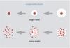 |
Fig. 1 Schematic showing the difference between the single-seed model and the many-seeds model for the internal structure of icy pebbles in the outer disk. In the single-seed model, the water ice layer (white) on the silicate core (red) becomes smaller at the evaporation front, and after complete evaporation of the ice, only one single silicate core remains. Since we take ζ = 0.5, the silicate core contains half the mass of the original pebble: mcore = mice = 0.5mp,start. In the many-seeds model, pebbles in the outer disk consist of many micron-sized silicate grains (red) “glued” together by water ice (white). As the ice evaporates, silicate grains are released as well. After complete evaporation of the ice, many micron-sized silicate grains remain. Again, with ζ = 0.5, the total mass in silicate grains in a pebble in the outer disk is half of the total pebble mass, but this mass is now divided among many silicate grains that each have mass msil. See text for more details. |
2.5. Transport equations
In this subsection we provide the systems of transport equations corresponding to both pebble composition models presented in Sect. 2.4. Our model is 1D; we integrate over the vertical dimension of the disk and follow column (surface) densities. Midplane densities are calculated assuming a Gaussian distribution in height with scaleheights Hgas (for the gas and the vapor) and Hpeb (for the pebbles), respectively.
2.5.1. Single-seed pebble model
In the single-seed model, we follow the vapor surface density ΣZ, the ice surface density Σice, and the number density of particles Np. The equations governing the time evolution of these quantities are: 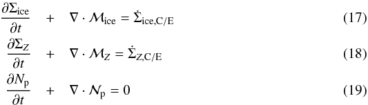 where the source terms
  and
and  are defined in Eqs. (12) and (15), ℳice and ℳZ are the ice and vapor mass flux, respectively, and
  is the number flux of solid particles. These fluxes are given by:
 where vpeb is the drift velocity of the pebbles given by Eq. (8) or by Eq. (B.7) when including collective effects, Ngas is the number of gas particles, and Dp is the particle diffusivity, which is related to Dgas through the Schmidt number Sc (Youdin & Lithwick 2007):
 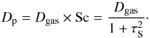 (23)Since in our models the stopping times are much smaller than unity, we set Dp equal to Dgas.
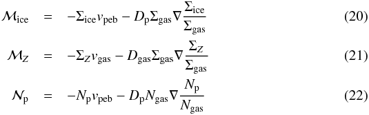
Note that a negative flux means that material is transported inwards, towards the star. Under the single-size approximation, the typical pebble mass mp is given by:  (24)with mcore the mass of the bare silicate cores of the pebbles.
2.5.2. Many-seeds pebble model
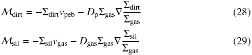
We implement the many-seeds model as follows. We now consider two additional populations of solids: dirt and free silicates. Dirt refers to the silicates that are captured in icy pebbles, whereas free silicates are small silicate grains without any ice coating. The transport equations for Σice, ΣZ, and Np are the same as in the single-seed pebble model (Eqs. (17)–(19)). The transport equations for the dirt surface density Σdirt and free silicates surface density Σsil are given by: ![Mathematical equation: \begin{eqnarray} \label{eq:transportDIRT} \frac{\partial \Sigma_{\rm{dirt}}}{\partial t} + \nabla \cdot \mathcal{M}_{\rm{dirt}} &=& - \rm{max}\left[ 0, ({\it R}_{\rm{e}} - {\it R}_{\rm{c}} \Sigma_{{\it Z}})\right] \Sigma_{\rm{dirt}} + {\it R}_{\rm{s}} \Sigma_{\rm{sil}}\\ \frac{\partial \Sigma_{\rm{sil}}}{\partial t} + \nabla \cdot \mathcal{M}_{\rm{sil}} &=& \rm{max}\left[ 0, ({\it R}_{\rm{e}} - {\it R}_{\rm{c}} \Sigma_{{\it Z}})\right] \Sigma_{\rm{dirt}} - {\it R}_{\rm{s}} \Sigma_{\rm{sil}}\\\nonumber \end{eqnarray}](/articles/aa/full_html/2017/06/aa30013-16/aa30013-16-eq92.png) where ℳdirt and ℳsil are the dirt and free silicate mass fluxes, respectively. Free silicates are released from the pebbles at a rate proportional to the decrease of ice surface density due to evaporation and to the amount of dirt that can evaporate from within the pebbles: (Re − RcΣvap)Σdirt, but only when there is net evaporation of ice. Silicate grains stick to icy pebbles at a collision/sticking rate Rs:
where ℳdirt and ℳsil are the dirt and free silicate mass fluxes, respectively. Free silicates are released from the pebbles at a rate proportional to the decrease of ice surface density due to evaporation and to the amount of dirt that can evaporate from within the pebbles: (Re − RcΣvap)Σdirt, but only when there is net evaporation of ice. Silicate grains stick to icy pebbles at a collision/sticking rate Rs:  (27)where Δvsil,peb is the relative velocity between the pebbles and the silicates and Hsil is the scale height of the free silicates. Since the inward drift velocity of the pebbles is much larger than the outward diffusion velocity of the silicates, we take Δvsil,peb ≈ vpeb2.
The dirt and silicate mass fluxes, ℳdirt and ℳsil, are given by:
 where vpeb is again the radial drift velocity of the pebbles, and silicates are advected with the gas.
2.6. Effects of variable μ
When icy pebbles evaporate, the gas becomes enriched in water vapor. This means that the mean molecular weight μ of the gas increases: 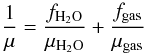 (30)where fH2O is the mass fraction of water molecules, μH2O = 18mH is the mean molecular weight of water, and fgas is the mass fraction of gas molecules (without the vapor contribution), with μgas = 2.34mH.
Since the sound speed cs is proportional to  , the sound speed decreases as more water vapor is added. The disk scale height Hgas is proportional to cs and will therefore decrease as well: the disk becomes more vertically compact with increasing water vapor. An increase in μ across the water evaporation front has an effect on the pebble drift velocity vpeb (Eq. (8)) in this region, since vpeb is proportional to 1 /μ through its dependence on cs, and sensitive to variations in the gas pressure P through ∂log P/∂log r. The total gas pressure (hydrogen/helium plus water) is given by:
 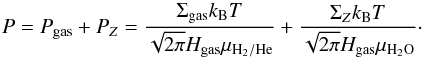 (31)We take the viscosity ν to be independent of variations in μ. Therefore, Σgas = Ṁgas/ 3πν is independent of μ as well. However, the H2O-enriched gas is characterized by a reduced scaleheight, since
  , increasing the midplane gas pressure Pgas as
  . Evaporation hence increases the pressure gradient and the headwind of the gas through Eq. (9): pebbles tend to drift faster. Finally, the drift velocity vpeb also depends on the stopping time τS, which in turn depends on the gas density and the thermal velocity – both quantities that depend on μ. We take these dependencies into account as well.
We now define two models that we study in the following sections. In the simple model, we do not include collective effects and the variability of the mean molecular weight μ. In the simple model, the sound speed and scale height are independent of variations in μ, ηvK (Eq. (9)) is constant and the midplane gas density is μ-independent:  . In the complete model, we do take collective effects and variations of μ into account, as described above.
2.7. Input parameters
The four key input parameters that can be varied in our model are:
-
The gas accretion rate Ṁgas.
-
The ratio between the pebble accretion rate and the gas accretion rate, denoted by the symbol ℱs / g, and defined as:
 (32)
(32) -
The dimensionless turbulence parameter α.
-
The initial stopping time of pebbles just outside the snowline (at 3 au) denoted by the symbol τ3. This parameter is simply a proxy for the mass of the incoming pebbles.
Together, these input parameters define the “zero-model” of the disk: the gas and solids distribution in the case of no condensation and evaporation. The gas surface density profile Σgas is defined through Eq. (4), where the turbulent viscosity ν is determined by α through Eq. (5). With Σgas and the stopping time normalization τ3 at 3 au, we can find τ(r) at any other radius r. We can then also determine the pebbles surface density Σpeb for the zero-model: it is given by ℱs / gṀgas/ 2πrvpeb(r), where the pebble velocity vpeb(r) depends on τ(r) and is given by Eq. (8) (without backreaction) or Eq. (B.7) (including backreaction).
2.8. Model assumptions
In constructing our model we employed several assumptions, which we discuss below.
-
We do not include a particle size distribution, but rather considerone typical pebble size at each time and location in the disk. In themany-seeds model, we do distinguish between the population ofsmall silicate grains and large icy pebbles, however. We comeback to the importance of condensation onto small grains ratherthan onto pebbles in the discussion (Sect. 6).
-
Our model does not account for coagulation among pebbles: the enhancement of the solids-to-gas ratio is solely due to diffusion and condensation. We remain agnostic as to what happens to the pebbles in terms of coagulation and fragmentation until they reach the evaporation front. In the many-seeds model, we do not take into account coagulation of silicate particles. We will come back to this point in the discussion (Sect. 6).
-
Our model is 1D, and has a straight vertical snowline. In reality, the vertical snowline is curved rather than straight, because the temperature varies with height above the midplane (e.g., Oka et al. 2011). However, Ros & Johansen (2013) have shown that particle growth due to diffusion and subsequent condensation of water across the vertical snowline is negligible compared to the same process across the radial snowline.
-
Similarly, we assume that the scale height of the vapor – and, in the many-seeds implementation, of the free silicates – is always equal to the scale height of the disk; in other words, when an icy pebble evaporates, the released water vapor immediately distributes itself over the same vertical extent as the background gas, whereas it originates from the icy pebbles that reside in a thinner disk, characterized by a scale height Hpeb:
 (33)The assumption of rapid vertical mixing extends to the calculation of the mean molecular weight of the gas in the complete model. Also there, it is assumed that the water vapor is distributed evenly throughout the gas at all times. In Sect. 4.2, we verify that the assumption of taking the vapor scale height equal to the disk scale height rather than the pebbles scale height, does not have a large effect on the results.
 -
We assume a steady-state gas distribution, that is, Ṁgas and T remain constant. This assumption is justified since the solids-to-gas enhancement takes place on a radial scale Δr that is small compared to the size of the disk. In other words, the local viscous evolution timescale (Δr2/ν), on which the effect happens, is much smaller than the global viscous evolution timescale of the disk, on which the gas accretion rate and global temperature profile change. The temperature profile (Eq. (1)) corresponds to a passively-irradiated disk. However, in case of viscous heating T(r) will still be described by a power-law (Armitage 2015). We have checked the effect of adopting a viscous heating temperature profile (T(r) ∝ r− 3 / 4) in our numerical simulation. The key consequence is that the location of the snowline is shifted in radius; all other model results are very similar.
-
We adopt an α-viscosity model, with constant α (the value of which we allow to vary between very high and very low values), independent of the solids-to-gas ratio. However, if turbulence is driven by the magneto-rotational instability, the local turbulence strength at the midplane depends on the local grain size and abundance. So-called “dead zones”, where turbulence is strongly reduced, could occur at locations in the disk with a sharp increase in the solids-to-gas ratio (Kretke & Lin 2007). Since our results depend strongly on the amount of turbulence near the snowline, the creation of dead zones would change our results.
-
Similarly, we do not consider the interplay between (small) grains and the local temperature: we do not solve for the temperature profile self-consistently, but take it as constant, given by Eq. (1). However, in the many-seeds model, a large amount of small silicate grains is released in the evaporation front. This means that locally the opacity could increase. Conceivably, this could lead to a steeper temperature profile in the region near the snowline and therefore to a more narrow evaporation front. Including these effects requires a radiation transfer model, which is beyond the scope of this work.
-
In the many-seeds implementation, we do not include condensation onto the small, free silicate particles. We also do not model the porosity of pebbles. We come back to these issues in Sect. 6.3.
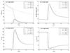 |
Fig. 2 The solution to the transport equations at different points in time, for the fiducial model parameters listed in Table 1. At t = 105yr, approximately 90% of the steady-state peak in the ice surface density has formed. a) Surface densities Σ of ice (solid lines) and vapor (dashed lines). The dotted line corresponds to the steady-state advection-only vapor surface density profile. b) Midplane pebbles-to-gas ratio ρpeb/ρgas. c) Typical pebble mass mp. d) Typical pebble internal density ρ•,p. |
3. Numerical implementation
We make use of the open source partial differential equations solver FiPy (Guyer et al. 2009) to solve the transport equations numerically. The coupled systems of equations are solved on a cylindrical 1D grid that ranges from 1 to 5 au.
We implement boundary conditions as follows. At the outer boundary r2 = 5 au, the pebble mass flux ℱs / gṀgas is fixed3. We convert the input parameter τ3 to a physical pebble size sp,start using Eq. (7), and since our model does not include coagulation, we set the pebble size (which can be converted to a pebble mass mp,start) at the outer boundary r2 to this value. For the single-seed model, the mass of the bare silicate core is then given by mcore = ζmp,start = mp,start/ 2. At the inner boundary r1 = 1 au, we implement outflow boundary conditions: solid particles and water vapor are accreted to the central star at a constant rate. We also demand that Σice = 0 at r1 and ΣZ = 0 at r2, for obvious reasons. Additionally, in the many-seeds implementation we have Σdirt = Σice = 0 at r1 and Σsil = ΣZ = 0 at r2.
3.1. Time-dependent
In our time-dependent method, we adopt small time steps (Δt ~ 100yr) and a small value for the allowed residuals, to ensure mass conservation by demanding the residuals4 to be small. This method requires a lot of computational power because the system of partial differential equations is numerically very stiff, but the advantage is that we find not only the steady-state solution to the equations, but are able to follow the solution in time. This allows us to get a measure of the time needed for the solution to settle into a steady-state. We present the time-dependent results for the “simple, single-seed” model with fiducial input parameters in Sect. 4.1.
3.2. Time-independent
Our time-independent method solves for the steady-state solution directly, by taking very large time-steps (in total 40 time steps that increase to 107yr) and decreasing the residuals threshold after each run, taking the solution from the previous run as the new input. We continue this process until we reach convergence. We present the steady-state results for the “simple, single-seed”, “simple, many-seeds”, “complete, single-seed”, and “complete, many-seeds” models with fiducial input parameters in Sect. 4.2.
4. Results – fiducial model
In this section we introduce a standard set of parameters which we then use to illustrate different aspects of the model. The fiducial model is defined by the parameters listed in Table 1. We first discuss the time-dependent results for the simple, single-seed, fiducial model in Sect. 4.1. We then go on to discuss the steady-state results for the other variants of the fiducial model in Sect. 4.2.
Fiducial model parameters.
4.1. Time-dependent solution
In Fig. 2 we plot several quantities as function of radial distance from the star r, at four points in time. In Fig. 2a, the surface densities of ice (solid lines) and vapor (dashed lines) are plotted. Initially (t = 0), the ice and vapor surface density are zero, Σice = ΣZ = 0. Icy pebbles are drifting in from the outer disk (right) to the inner disk (left). At the point where  the icy component of the pebbles evaporate. At the snowline rsnow ≈ 2.1 au all the H2O is in the gas phase. Since the vapor is advected with the gas velocity vgas, which is much smaller than the pebble velocity vpeb, the vapor surface density (dashed line) quickly exceeds that of the ice (solid line). The vapor density increases until the steady-state vapor distribution ΣZ,a has been reached. ΣZ,a is given by5:
  (34)and is plotted by the dotted curve. Meanwhile, due to the outward diffusion of water vapor across the snowline and subsequent condensation onto the inward-drifting pebbles, the ice surface density just exterior to the snowline increases. Diffusion of vapor therefore results in a distinct bump in the ice profile and we denote the location corresponding to maximum Σice the peak radius rpeak. A similar maximum is seen in the solids-to-gas ratio (Fig. 2b), which rises to ~0.45. After t = 2 × 10⁵ yr a steady state has been reached.
The enhancement of the pebbles-to-gas ratio is reflected by the typical pebble mass mp and density ρ•,p, plotted in Figs. 2c and d, respectively. Pebbles at the inner boundary are half as massive as pebbles at the outer boundary, because at the inner boundary all the ice has evaporated off the pebbles, and the dust fraction of pebbles ζ = 0.5. The typical pebble mass just outside the snowline increases over time, indicating that water vapor condenses onto the pebbles. This is also shown by the behavior of the typical pebble density ρ•,p. At the outer boundary, ρ•,p = 1.5gcm-3, corresponding to pebbles containing as much water ice as silicates in mass; at the inner boundary, ρ•,p = 3gcm-3, corresponding to pure silicate pebbles; whereas just outside the snowline, ρ•,p decreases over time to values close to unity – corresponding to pure water ice pebbles. A decrease in particle internal density outside the snowline due to water condensation was also found by Estrada et al. (2016).
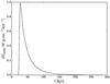 |
Fig. 3 Rate of change of the ice surface density at the peak location, as function of time. The rate of change increases until the icy pebble front has reached the peak location, after which the peak continues to grow at an exponentially decreasing rate, while the system is converging to its steady-state solution. |
In Fig. 3 we plot the growth rate of the peak in Σice outside the snowline as function of time t. At the start of the simulation, ice is not yet present at the location of the peak. After the icy pebbles have reached the location of the eventual peak, at t ~ 2 × 10⁴yr, the rate of growth decreases exponentially – the peak continues to grow, but at an ever slower rate, while the system is converging to its steady-state solution. The e-folding growth timescale is ~3 × 10⁴yr, which is approximately equal to the gas advection timescale (rpeak − rsnow) /vgas; the time it takes for the vapor to traverse the peak and contribute to the steep vapor concentration gradient along which outward diffusion can take place. We will come back to the peak formation timescale in Sect. 5. The time in which 90% of the peak forms is ~105yr. Note that we have assumed that the incoming pebble mass flux does not change over time (ℱs / g is constant at the outer boundary r2). If the pebble flux would decrease on a timescale shorter than the time it takes to form the peak, a steady-state would not exist. If the pebble flux would decrease on a timescale longer than it takes to form the peak, we would reach a quasi-steady-state solution; in that case our model is fully applicable.
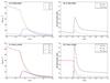 |
Fig. 4 Steady-state results for the fiducial parameters, for the simple model with single-seed evaporation (upper two panels) and many-seeds evaporation (lower two panels). a) Surface densities of ice, silicates and vapor (Σice, Σsil, and ΣZ, respectively) for the single-seed model. The silicates are locked in the icy pebbles outside the snowline, whereas they are bare grains interior to the snowline. b) Midplane pebbles-to-gas ratio ρpeb/ρgas, and pebbles-to-gas column density ratio Σpeb/ Σgas for the single-seed model. c) Same as panel a) but for the many-seeds model. The silicates are now divided in two populations: silicates that are locked up in icy pebbles (Σdirt), and free silicates (Σsil). Note that in panels a) and c) the x-axis ranges between r = 1.8 − 2.8au, for clarity. d) Same as b), but for the many-seeds model and with an additional line for the midplane “free silicates”-to-gas ratio ρsil/ρgas. |
4.2. Steady-state solution
The time-dependent solution described in Sect. 4.1 converges to the steady-state solution. In this section we take a closer look at the steady-state solution for the fiducial parameters, for the model designs discussed in Sect. 2.
4.2.1. Single-seed versus many-seeds
In Fig. 4 we compare the simple single-seed model (upper two panels) with the simple many-seeds model (lower two panels). The left panels show the surface densities of ice, vapor, and in the many-seeds case, also of locked silicates (dirt) and free silicates. The ice profiles are very similar in both models, but in the many-seeds case there is an additional peak in the dirt surface density. This is because the free silicates behave like vapor: they are released throughout the evaporation front, and follow the gas profile interior to the snowline. Turbulent diffusion not only causes vapor to be transported outward and condense onto the pebbles, but leads to the same effect for the small silicates – they diffuse outward and stick onto the pebbles, resulting in a peak in the dirt surface density distribution.
In the right panels we plot pebbles-to-gas midplane density ratios ρpeb/ρgas and column density ratios Σpeb/ Σgas. In the many-seeds model, the pebbles-to-gas ratio is the sum of the dirt-to-gas ratio and the ice-to-gas ratio. In both models, a clear peak is present just outside the snowline. The midplane density ratio is larger than the column density ratio due to settling of pebbles. In the many-seeds case, we also plot the free silicates-to-gas midplane density ratio ρsil/ρgas. This ratio is constant interior to the snowline because the silicates are perfectly coupled to the gas. In the many-seeds model, small silicate grains diffuse outward across the snowline, whereas in the single-seed model, there is no significant outward diffusion of the larger silicate pebbles due to the absence of a steep concentration gradient. Therefore, the peak in the pebbles-to-gas ratio outside the snowline is larger in the many-seeds model than in the single-seed model.
4.2.2. Simple versus complete models
Figure 5 shows the results for the complete model with the single-seed pebble design (upper two panels, a and b) and with the many-seeds pebble design (lower two panels, c and d). In Fig. 5a (single-seed) and Fig. 5c (many-seeds), we plot the surface densities of ice, vapor, and in the many-seeds case the surface densities of locked silicates (dirt) and free silicates (sil). Dashed lines denote the simple model results of Figs. 4a and c, for comparison. The grey lines correspond to the mean molecular weight of the gas. From the outer disk to the inner disk, the mean molecular weight increases from 2.34 mH to 3.11 mH across the snowline. Clearly, the peak in the ice surface density is higher and broader for the complete model than for the simple model. This is because collective effects (which reduce the pebble drift velocity) outweigh the effect of the enhanced gas pressure gradient in the evaporation front (which enhances the pebble drift velocity). In the complete model, therefore, pebbles effectively have a smaller radial velocity than in the simple model, and therefore the resulting ice peak is higher and broader. This is also the case in the many-seeds implementation. The width of the peak strengthens the justification of the vertical mixing assumption (see below).
In Figs. 5b and d we compare the midplane pebbles-to-gas ratios between the simple and the complete model. Collective effects help to boost the pebbles-to-gas ratio, for the reason outlined above.
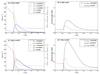 |
Fig. 5 Comparison of steady-state results for the fiducial parameters between the simple model (dashed lines) and the complete model (solid lines), which includes collective effects and the effects of the variation of the mean molecular weight μ. The upper two panels correspond to the single-seed evaporation model; the lower two panels correspond to the many-seeds evaporation model. In the latter case, we made the conservative choice of not including the free silicates in the back-reaction onto the gas. a) Surface densities of ice (Σice), vapor (ΣZ) and silicates (Σsil) for the single-seed model. The grey line indicates the mean molecular weight of the gas in units of proton mass mH. b) Midplane pebbles-to-gas ratio ρpeb/ρgas. c) Same as a), but the silicates are now divided into “free silicates” (Σsil) and “locked silicates” (Σdirt). For clarity, we only show the clean Σice profile for comparison. d) Same as b), with an additional line denoting the “free silicates”-to-gas ratio ρsil/ρgas. |
4.2.3. Validation of vertical mixing assumption
As discussed in Sect. 2.8, we assume rapid vertical mixing of vapor. However, it could be argued that (part of) the released vapor recondenses onto icy pebbles before relaxing to the same vertical distribution as the gas, thereby boosting the condensation rate. This assumption also extends to the small silicate grains in the many-seeds model. Similarly, one could argue that the silicate grains can collide with a pebble before they can diffuse to higher vertical layers (e.g., Krijt & Ciesla 2016). In order to investigate what the difference is in terms of the steady-state ice distribution between two extreme cases, we take the simple, single-seed, fiducial model and run it once with HZ = Hgas and once with HZ = Hpeb. We compare the steady-state outcomes of the two cases in Fig. 6. Even though the location of the snowline and of the pebbles-to-gas peak differs a bit between the two cases, the height of the peak in the midplane pebbles-to-gas ratio increases only by ~0.3% if one takes HZ = Hpeb instead of HZ = Hgas. Similarly, assuming a smaller scale height for the silicate grains in the evaporation region would probably not significantly change the height of the peak in the “locked” silicates, since the silicate grains behave like vapor. In the rest of this paper, we assume HZ = Hsil = Hgas.
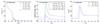 |
Fig. 6 Comparison of steady-state results for the simple, single-seed, fiducial model between the case where vapor has the same vertical distribution as the background gas (HZ = Hgas) and the case where vapor has the same scale height as the pebbles (HZ = Hpeb). In all three panels, solid lines correspond to the HZ = Hgas case and dashed lines correspond to the HZ = Hpeb case. a) Steady-state water ice (blue) and water vapor (green) surface densities. b) Midplane solids-to-gas ratios (green) and solids-to-gas surface densities ratios (blue). c) Typical pebble mass mp. |
5. Streaming instability conditions
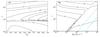 |
Fig. 7 a) Contours of constant relative ice surface density peak heights fΣ,peak (see text for details) as function of turbulence parameter α and solids-to-gas accretion rate ℱs / g. The gas accretion rate Ṁgas is fixed to 10-8M⊙yr-1 and the initial size of the pebbles τ3 is fixed to 0.03. b) Contours of constant relative ice surface density peak heights (see text for details) as function of the turbulence parameter α and the gas accretion rate Ṁgas. The solids-to-gas accretion rate ratio ℱs / g is fixed to 0.4 and the initial size of the pebbles τ3 is fixed to 0.03. The cyan lines denote a Toomre parameter (QT) of unity at 10 au (1 au); the space below these lines has QT< 1 and is gravitationally unstable at 10 au (1 au). |
Carrera et al. (2015) have investigated for what values of the solids-to-gas column density ratio streaming instability occurs, as function of the stopping time of the solid particles. They found that, typically, the solids-to-gas column density ratio should exceed ~2% for stopping times ~5 × 10⁻². However, these results should be interpreted with caution, since Carrera et al. (2015) only accounted for self-driven (Kelvin-Helmholtz) turbulence. We do include global turbulence, and therefore cannot simply use their conditions for streaming instability. A more robust condition for streaming instability in the presence of global turbulence is probably a midplane solids-to-gas ratio that reaches order unity (Johansen & Youdin 2007).
In this section we investigate under what disk conditions, the midplane solids-to-gas ratio near the snowline gets most enhanced due to the effect of water diffusion and condensation. To this end, we have constructed a semi-analytic approximate model to be able to quickly test for many different values of the input parameters (Sect. 2.7), within the single-seed implementation (Sect. 2.4). Before presenting the results, we will provide a short summary of the semi-analytical model, which is discussed in greater detail in Appendix C.
5.1. Semi-analytical model: Summary
Our semi-analytical model is an analytic prescription to find the approximate location, height and width of the ice surface density at the location of the ice peak, rpeak, of the steady-state (time-independent) solution (see Sect. 3.2 for our numerical method to find the steady-state solution to the transport equations). For simplicity, we have tailored the semi-analytical model towards the “single-seed” design. (An extension to also include the “many-seeds” design will be considered in a future work.)
The model works by iteratively solving a set of analytical equations, until convergence is reached. The key parameter is the ratio between the pebble velocity at rpeak and the normalized diffusivity at this location, ϵ = vpeb(rpeak) /D(rpeak)rpeak. Initially, we start with an estimate for ϵ, which can, for example, be taken from the zero-model solution (Sect. 2.7). For a certain ϵ the semi-analytical model then updates the surface density at the peak (Σpeak) as well as rpeak (or rather the difference between rice and rpeak). With these updates we obtain a new value of ϵ and the procedure can be repeated until the fractional change in the parameters has become sufficiently low.
We emphasize that the semi-analytical model gives approximate solutions (correct at the ~20% level), but that they are very useful since they come at almost zero computational costs. It is therefore ideal to be applied to the parameter searches that we consider in this section. In Appendix C the model is described in detail and compared to runs of the numerical steady-state model.
5.2. Enhancement of the ice surface density
We first look at the relative effect of enhancing the ice surface density near the snowline: for each disk model, we normalize the resulting peak ice surface density by the ice surface density at the peak radius in case there is only advection:  (35)where vpeb is calculated in the absence of condensation and evaporation. As before, we take ζ = 0.5. In Fig. 7a we plot contours of constant fΣ,peak as function of α and ℱs / g, where Ṁgas is fixed at 10-8M⊙yr-1 and τ3 is fixed at 0.03. Clearly, the higher the solids-to-gas accretion rate ℱs / g, the higher fΣ,peak – at fixed α the normalized ice peak increases from low ℱs / g-values to high ℱs / g-values, due to collective effects playing an increasingly important role. The plot also shows that disks with α-values of about 10-3 are best at enhancing the ice surface density with respect to the advection-only expected ice surface density. This is because higher values of α lead to a broader and relatively lower peak, while lower α-values, indicating larger gas densities, move pebbles into the Stokes drag regime. The fact that the relative height of the ice peak becomes smaller when pebbles enter the Stokes regime, is explained by the pebble size-dependency of the drift velocity. In the Epstein regime the drift velocity depends linearly on the pebble size, whereas in the Stokes regime the drift velocity is proportional to the square of the pebble size. This means that when pebbles enter the Stokes regime, their stopping time – and hence their drift velocity – increases rapidly. The effect of this is that fΣ,peak decreases rapidly. Therefore, the transition from the Epstein regime to the Stokes drag regime is characterized by closely-spaced contours.
Figure 7b shows contours of constant fΣ,peak, as function of α and Ṁgas. ℱs / g is fixed at 0.4 and τ3 is fixed at 0.03. The cyan lines correspond to a Toomre parameter (QT) of unity at 10 au (1 au). QT is defined as:  (36)where G is the gravitational constant. A disk is gravitationally unstable if QT< 1. In Fig. 7b, models in the parameter space below the cyan line have QT< 1 at 10 au (1 au). In Fig. 7b densely-spaced contours again indicate the transition between Epstein and Stokes drag.
The enhancement of the ice surface density near the snowline is relatively modest, but enrichment factors of a few can still be important for triggering streaming instability (Johansen et al. 2009). Besides, Fig. 7 corresponds to our single-seed model, which is conservative. Larger enhancements can be achieved in the framework of the many-seeds model (see Fig. 4). We can imitate the many-seeds model in the analytical model of Appendix C, crudely, when we let ζ → 0, which assumes that micron-sized silicate grains behave like vapor. In that case we see fΣ,peak increase by another factor of two (results not plotted). Therefore, total enhancements of fΣ,peak ~ 5–10 are feasible, which significantly boost the likelihood of triggering streaming instability.
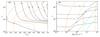 |
Fig. 8 a) Contours of midplane solids-to-gas ratios (black) as function of the turbulence parameter α and the solids-to-gas accretion rate ℱs / g. The gas accretion rate Ṁgas is fixed to 10-8M⊙yr-1 and the initial size of the pebbles τ3 is fixed to 0.03. Orange contours denote the amount of solid material (in Earth masses) that is required to form the eventual peak in the ice surface density just outside the snowline. b) Contours of midplane solids-to-gas ratios as function of α and Ṁgas. The solids-to-gas accretion rate ℱs / g is fixed to 0.4 and the initial size of the pebbles τ3 is fixed to 0.03. Orange contours denote the amount of solid material (in Earth masses) that is required to form the eventual peak in the ice surface density just outside the snowline. The cyan lines denote a Toomre parameter (QT) of unity at 10 au (1 au); the space below these lines has QT< 1 and is gravitationally unstable at 10 au (1 au). |
5.3. Solids-to-gas ratios
Let us now look at the absolute results, in terms of the midplane solids-to-gas ratio. In Fig. 8a, black lines denote contours of constant peak midplane solids-to-gas ratios, as function of α and ℱs / g. We again fix Ṁgas = 10-8M⊙yr-1 and τ3 = 0.03. The orange contours correspond to the total amount of solids in units of Earth masses that is needed to form the eventual peak. This quantity (Msolids,needed) is calculated as: 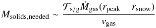 (37)where (rpeak − rsnow) /vgas is the typical timescale on which the peak forms, as discussed in Sect. 4.1. The value of Msolids,needed is similar to the amount of solids that gets “locked up” in the peak6. Figure 8a shows that the higher the value of ℱs / g, the easier streaming instability can be triggered, as one may expect. It also shows that in order to reach midplane solids-to-gas ratios of ~10%, a solids-to-gas accretion rate ℱs / g of the same order is required. This also holds for other values of the gas accretion rate Ṁgas and initial pebble size τ3.
Figure 8b is the same as Fig. 7b, except that the black contours now denote constant values of the peak midplane solids-to-gas ratio. Just like in Fig. 8a, orange contours denote constant Msolids,needed, but now with Ṁgas as the parameter on the x-axis. The region with closely-spaced contours in Fig. 8a and the oblique regions in the otherwise fairly horizontal contours in Fig. 8b are again due to the transition between the Epstein and Stokes drag regimes.
Up to this point we have kept the parameter τ3 constant at its fiducial value of 0.03. Recently, Yang et al. (2016) have shown that the streaming instability mechanism can also work for small particles (τ ~ 10-3). In Fig. 9 we now vary τ3 and plot the resulting peak midplane solids-to-gas ratio, whilst fixing Ṁgas at 10-8M⊙yr-1, ℱs / g at 0.4, and α at 3 × 10⁻³. Different regimes in the plot are denoted by Roman numbers I–IV. In region I, the particles are well-coupled to the gas. The solids-to-gas ratio flattens out towards low τ3-values, because radial drift and settling do not play a role for these particles. The boundary between regime I and regime II corresponds to the value of α. The highest solids-to-gas ratios are reached for particles with stopping times of the same order as α or smaller. For higher values of τ, the larger drift velocity (proportional to τ) starts to dominate over the larger degree of settling (proportional to  ). Therefore, in regime II, the solids-to-gas ratio decreases with increasing τ. The transition from regime I and regime II corresponds to the τ3-value for which ϵ is unity. The ϵ parameter (introduced in Sect. 5.1) increases with increasing τ3, and the peak surface density decreases at a faster rate with increasing ϵ for ϵ> 1 than for ϵ< 1 (Eq. (C.13)). The physical explanation is that the solution changes from diffusion-dominated (ϵ< 1) to drift-dominated (ϵ> 1). Therefore, the solids-to-gas ratio decreases more steeply in regime III than in regime II. The final transition, from regime III to regime IV, is caused by the transition from the Epstein regime to the Stokes regime. For τ3 values of ~1, the enhancement effect becomes minimal and the peak solids-to-gas ratio flattens out.
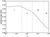 |
Fig. 9 Peak midplane solids-to-gas ratio as function of τ3. Ṁgas is fixed at 10-8M⊙yr-1, ℱs / g at 0.4, and the value of α is 3 × 10⁻³. We can distinguish four regimes I–IV, which are explained in the main text. |
From Figs. 8a and b we learn that in the context of the α-viscosity disk model, the largest solids-to-gas ratios near the snowline are reached for high α-values. This means that our diffusion model does not require a very quiescent disk to achieve high solids-to-gas ratio, and also works in the early disk phase when α and Ṁgas are presumably high. Our results show that for high α and high Ṁgas, tens of Earth masses are locked up in pebbles in an annulus outside the snowline with a width of the order of 1 au.
6. Discussion
6.1. Conditions for streaming instability
Our results show that the ice surface density can be enhanced by a factor ~3–5 outside the snowline, due to the effect of water diffusion and subsequent condensation onto icy pebbles (adopting ζ< 0.5 or the many-seeds model increases the enhancement by another factor ~2). This differs from the results of Stevenson & Lunine (1988), who found that the same effect could lead to an enhancement by as much as 75. However, they considered a static system, whereas our model accounts for radial drift of pebbles and gas accretion onto the star. Even though we found a modest enhancement, we showed that the pebble density at the midplane can reach tens of percent of the gas density, under the condition that the solids-to-gas accretion rate ℱs / g is of order 0.1.
But what are realistic values for ℱs / g? Ida et al. (2016) have calculated the pebble mass flux Ṁpeb in a viscously-evolving disk, taking into account dust growth and radial drift. They found that after 106 yr, ℱs / g ~ 0.3 for a turbulence parameter α = 10-3 and a gas accretion rate Ṁgas = 10-8M⊙yr-1. Since this result suggests ℱs / g-values of order 0.1 are plausible, water condensation can plausibly trigger streaming instability near the snowline. According to Ida et al. (2016), Ṁpeb is inversely proportional to α. This implies that even though our results show that for high α-values, water diffusion and condensation leads to the largest solids-to-gas ratio at the snowline, a smaller pebble mass flux is expected, which reduces the effect. The pebble mass flux is, however, dependent on time t as Ṁpeb ∝ t− 1 / 3, meaning that the pebble mass flux earlier in the disk is higher than the fiducial 30% of the gas accretion rate quoted before. Because higher α-values lead to larger solids-to-gas ratios but to lower pebble mass fluxes, we conclude that intermediate α-values (~10-3) are most favorable to trigger streaming instabilities. The fact that the diffusion-driven model of this work already produces enhancement of solids at intermediate α-values and high Ṁgas, implies that planetesimal formation does not have to await the arrival of quiescent disk conditions. Provided a sufficiently large pebble flux, our results imply that planetesimals can form early.
6.2. Interior or exterior?
In Saito & Sirono (2011), it is argued that the evaporation of icy pebbles leads to a large enhancement of small silicate grains interior to the snowline. In their model, micron-sized silicate grains are instantaneously released at the snowline, and then follow the radial motion of the gas. Since the gas moves at a much lower velocity than the drift velocity of the icy pebbles, the silicate grains pile-up and become gravitationally unstable. A similar mechanism for the formation of planetesimals in the inner disk has recently been presented by Ida & Guillot (2016).
We confirm that the solids-to-gas ratio interior to the snowline is boosted due to the slow radial motion of the small silicates (see Fig. 4c), but find smaller enhancements than Saito & Sirono (2011) and Ida & Guillot (2016). These works assumed that the evaporated silicate grains remained in the same vertical layer as the icy pebbles, which had settled to the midplane due to their larger size. This is a natural assumption if one adopts instantaneous evaporation. However, in our model silicate grains are not instantaneously released from the pebbles at a single location, but are instead released across the ice evaporation front – the region between the snowline and the peak radius. With the exception of very low α-values, the width of the ice peak is (much) larger than the gas scale height. Consequently, the timescale for vertical mixing is smaller than the timescale on which the silicate grains traverse the evaporation front, justifying our assumption that silicate grains (and water vapor) are distributed over Hgas. Allowing for the vertical mixing of silicate grains is why we found smaller solids-to-gas ratios interior to the snowline than Saito & Sirono (2011) and Ida & Guillot (2016).
In this work we did not model the porosity of pebbles, but assumed pebbles are compact spheres. For homogeneous porous spheres, the results are the same as for compact spheres with the same stopping time, if they are in the Epstein regime. This is because the evaporation and condensation rates (Eqs. (13), (14)) depend on  (the surface to mass ratio of a pebble), which is effectively the Epstein stopping time (Eq. (7)). For fractal aggregates, however, the evaporation rate could conceivably be increased due to a larger total surface area available for evaporation. In that case, the location of the snowline (rsnow) and of the peak (rpeak) are pushed to larger radial distances, because drifting pebbles start to evaporate earlier. The shape of the solids distribution profile and hence the width of the evaporation front, however, remain similar. We have confirmed this behavior by running our simulation with an evaporation rate that has been arbitrarily increased by a factor 100 compared to Eq. (13). Therefore, a fractal interior structure of the pebbles would not much change the extent of the region in which pebbles evaporate. We note however that in the many-seeds model, a large increase in opacity due to small silicate grains might lead to a steeper temperature profile than assumed here, and therefore to a more narrow evaporation front.
Even though we found smaller enhancements interior to the snowline, adopting the many-seeds model leads to larger enhancements outside the snowline compared to the single-seed model. This is because outward radial diffusion and subsequent sticking of silicate grains to icy pebbles adds to the ice peak and therefore enforces the enhancement of the solids-to-gas ratio outside the snowline (see Fig. 5).
6.3. Condensation onto small grains
In our single-seed model, we adopted a single-size assumption for the solid particles, applicable to a drift-limited scenario, in which particles grow until they decouple from the gas and start to drift inward (see, e.g., Birnstiel et al. 2010; Krijt et al. 2016b). Because the solids density is larger close to the star than in the outer disk, particles close to the star start to drift inward earlier than particles in the outer disk. This leads to an inside-out clearing of the solids component of the disk. In this case, one would not expect small particles to be present in significant amounts near the snowline at the time when icy pebbles approach the snowline, drifting in from the outer disk. Therefore, in the drift-limited case the single-size approximation for pebbles is valid.
The single-size assumption does not hold for a fragmentation-limited size distribution, however. In that case, pebbles dominate the total mass of solids, but small particles dominate the total surface area (see, e.g., Birnstiel et al. 2012). Then, condensation of water vapor will predominantly happen onto small particles, instead of onto pebbles as considered in this work. Also, in our many-seeds model, we do not allow for condensation onto the small grains that get released from icy pebbles upon evaporation.
Within the single-seed framework, we can mimic the situation where condensation happens onto small grains rather than onto pebbles by adopting a very small typical stopping time just outside the snowline (τ3). This results in approximately the same or even larger peaks, as illustrated by Fig. 9. In that sense, assuming condensation occurs solely onto pebbles, rather than onto small grains, is a conservative choice. However, a more correct approach would allow for condensation onto small grains in the many-seeds model, in which icy pebbles break up into small grains upon evaporation, or, alternatively, within a fragmentation-limited scenario by adopting a full size distribution. Such improvements will be considered in future work.
6.4. Relevance of coagulation
The many-seeds model ignores coagulation among the small silicate grains, as well as the possibility that water vapor condenses on to silicates. Because there are so many of them, the average silicate grain size would not increase significantly due to water condensation. In that case, the assumption that they are well-coupled to the gas would still hold. However, growth of silicates might also occur due to coagulation. Growth increases the drift velocity, thereby reducing the effect of the outward-diffusion and recondensation of the silicate component. Consequently, coagulation among silicates would bring the many-seeds model closer to the single-seed model due to a decrease in the enhancement of “locked” silicates outside the snowline. A similar trend is expected when the silicates that are released upon evaporation are larger. According to the experimental work of Aumatell & Wurm (2011), an icy aggregate of 1 cm in size breaks up into about 200 sub-aggregates when it evaporates. In any case, we expect that a more realistic “break-up” or coagulation model will lead to results that lie in between the results for our many-seeds and single-seed model designs.
In our work, we have also neglected coagulation among pebbles. On the one hand, one could think that icy pebbles on their way to the snowline would grow even more because of coagulation – at least as long their relative velocities stay low enough. On the other hand, according to Sirono (2011) and Okuzumi et al. (2016), the fragmentation threshold velocity for icy pebbles near the snowline is reduced due to sintering. This might motivate a smaller average icy pebble size (a lower τ3 in our nomenclature) and therefore a smaller radial drift velocity, which would further increase the solid surface density exterior to the snowline (see Fig. 9).
6.5. Observational implications
We showed that intermediate-to-high α-values are most favorable for triggering streaming instability near the snowline. The onset of streaming instability manifests itself through the formation of a peak in the solids-to-gas ratio that grows in height (increasing Σice) but also in width – the latter because collective effects cause pebbles to move slower. Even though more solids are required for high α and high Ṁgas than for low α and low Ṁgas, tens of Earth masses are sufficient to form the ice peak. This also means that tens of Earth masses can be stored in an annulus outside the snowline, especially when the system is characterized by high pebble and gas accretion rates. Such annuli of solid enhancement can be observable with facilities as ALMA. In the context of the snowline, the ring structure seen in the TW Hya system with a width of about 1 au (Andrews et al. 2016) might very well correspond to a realisation of the water-diffusion effect in a highly turbulent disk with a high gas accretion rate.
The fact that the planets in the inner solar system are water-poor (Marty 2012; McCubbin et al. 2012), even though the snowline should have migrated to 1 au before the disk was depleted, was pointed out as the “snowline problem” by Oka et al. (2011). The early formation of a protoplanet near the snowline might provide a solution to this problem, as proposed recently by Morbidelli et al. (2016). Once a protoplanet near the snowline has formed it could halt the inward-drifting pebble flux, either by accreting the pebbles (Guillot et al. 2014), or by trapping them in pressure maxima created by the newborn planet (Zhu et al. 2014; Lambrechts et al. 2014). In the meantime, the water vapor gets accreted to the star and the snowline location migrates inward (e.g., Oka et al. 2011). Consequently, an early formation of a protoplanet near the snowline might explain the lack of water in the inner solar system. The water diffusion/condensation effect discussed in this paper provides a way to form planetesimals near the snowline in an early stage of the disk (i.e., when the snowline is still located outside of the current water-poor region of the solar system). After planetesimals of a certain size have formed, they can subsequently accrete pebbles and quickly grow to larger bodies (e.g., Ormel & Klahr 2010; Lambrechts & Johansen 2012, 2014; Bitsch et al. 2015; Visser & Ormel 2016). Therefore, our water diffusion/condensation model provides the first key step to realize the early formation of a protoplanet near the snowline.
7. Conclusions
Our main findings can be summarized as follows.
-
1.
Water diffusion and condensation near the snowline can resultin an enhancement of a factor several in the ice surface density.Because of the dynamic setup of our model where water vapor iscarried away with the accreting gas, this enhancement is muchless than found by Stevenson & Lunine (1988).Nevertheless, the boost in the solids-to-gas ratio can still triggerstreaming instability, provided a large enough pebble flux.
-
2.
The peak in the ice surface density is not located at the snowline, but exterior to it (rpeak>rsnow). With larger incoming pebble flux, the peak becomes broader, because the back-reaction of the solids on the gas reduces the pebble drift velocity. Depending on the turbulence strength, the width of the peak can be as much as ~1 au.
-
3.
Such broad peaks can contain tens of Earth masses in pebbles, appearing as bright annuli at radio wavelengths.
-
4.
The release of many micron-sized silicate grains upon evaporation of icy pebbles produces a peak in “locked” silicates exterior to the snowline, due to diffusion and sweep-up of the silicates. This peak adds to the ice peak and therefore enforces the enhancement of the solids-to-gas ratio outside the snowline.
-
5.
Interior to the snowline, the solids-to-gas ratio is boosted if many micron-sized silicate grains are released during evaporation, because they cause a “traffic jam” effect. However, because silicate grains mix with the background gas before they cross the snowline, the solids-to-gas ratio enhancement just interior to rsnow is limited.
-
6.
In the context of a viscous disk model, the ratio between the accretion rate of solids and gas needs to be of order ~0.1 in order to reach solids-to-gas midplane ratios of the order of tens percent. The mechanism operates best at intermediate (~10-3) α-values. Therefore, planetesimals can form at an early time in the evolution of the disk.
Dra¸żkowska et al. (2016) argue that growth and radial drift can lead to pile-ups in the inner disk, where streaming instability may then be triggered. Recently, Gonzalez et al. (2017) also presented a pile-up mechanism.
For simplicity, we have ignored other contributions to Δvsil,peb. Turbulent velocities, however, may dominate over radial drift motion when α is large (Cuzzi & Hogan 2003; Ormel & Cuzzi 2007). Accounting for turbulent relative velocities will result in an increase of the peak solids-to-gas ratio of ~10% (e.g., 20% for our fiducial parameters presented in Table 1).
We do not fix the pebble surface density: for high values of α, outward diffusion can be strong enough to enhance the surface density of pebbles at the outer boundary (Σpeb,r2) with respect to the expected value Σpeb,r2 = Ṁpeb/ (2πr2vpeb(r2)) in case of no diffusion.
FiPy linearizes the equations while our system is nonlinear; the residuals quantify this mismatch.
Diffusion does not play a role in the steady-state, advection-only vapor surface density profile, because vapor has the same velocity as the gas and therefore the vapor concentration is independent of r.
We stress again that the model assumes that the incoming pebble mass flux is constant over time (see Sect. 4.1). However, the amount of solids needed to form the peak is independent of this assumption.
Taylor-expansion of the exponent, on the other hand, would be valid only over a very limited range, because aeq ≫ 1.
For p ≠ 0 a closed-form solution is possible but extremely contrived.
Acknowledgments
D.S. and C.W.O. are supported by the Netherlands Organization for Scientific Research (NWO; VIDI project 639.042.422). We would like to thank Jonathan Guyer and Daniel Wheeler for their elaborate answers to FiPy-related questions. We would also like to thank Carsten Dominik, Shigeru Ida, Satoshi Okuzumi, Anders Johansen, Daniel Carrera and the other participants of the Lorentz workshop “New directions in Planet Formation” (Leiden, July 2016) for stimulating discussions. We are indebted to Sebastiaan Krijt, Jeff Cuzzi, and the anonymous referee for constructive feedback on the manuscript.
References
- ALMA Partnership,Brogan, C. L., Pérez, L. M., et al. 2015, ApJ, 808, L3 [NASA ADS] [CrossRef] [Google Scholar]
- Andrews, S. M., Wilner, D. J., Zhu, Z., et al. 2016, ApJ, 820, L40 [NASA ADS] [CrossRef] [Google Scholar]
- Armitage, P. J. 2015, ArXiv e-prints [arXiv:1509.06382] [Google Scholar]
- Armitage, P. J., Eisner, J. A., & Simon, J. B. 2016, ApJ, 828, L2 [NASA ADS] [CrossRef] [Google Scholar]
- Aumatell, G., & Wurm, G. 2011, MNRAS, 418, L1 [NASA ADS] [CrossRef] [Google Scholar]
- Bai, X.-N., & Stone, J. M. 2010, ApJ, 722, 1437 [NASA ADS] [CrossRef] [Google Scholar]
- Banzatti, A., Pinilla, P., Ricci, L., et al. 2015, ApJ, 815, L15 [NASA ADS] [CrossRef] [Google Scholar]
- Benz, W. 2000, Space Sci. Rev., 92, 279 [NASA ADS] [CrossRef] [Google Scholar]
- Birnstiel, T., Dullemond, C. P., & Brauer, F. 2010, A&A, 513, A79 [NASA ADS] [CrossRef] [EDP Sciences] [Google Scholar]
- Birnstiel, T., Klahr, H., & Ercolano, B. 2012, A&A, 539, A148 [NASA ADS] [CrossRef] [EDP Sciences] [Google Scholar]
- Bitsch, B., Lambrechts, M., & Johansen, A. 2015, A&A, 582, A112 [NASA ADS] [CrossRef] [EDP Sciences] [Google Scholar]
- Blum, J., & Wurm, G. 2000, Icarus, 143, 138 [NASA ADS] [CrossRef] [Google Scholar]
- Brauer, F., Henning, T., & Dullemond, C. P. 2008, A&A, 487, L1 [NASA ADS] [CrossRef] [EDP Sciences] [Google Scholar]
- Carrera, D., Johansen, A., & Davies, M. B. 2015, A&A, 579, A43 [NASA ADS] [CrossRef] [EDP Sciences] [Google Scholar]
- Chapman, S., & Cowling, T. 1970, The Mathematical Theory of Non-uniform Gases: An Account of the Kinetic Theory of Viscosity, Thermal Conduction and Diffusion in Gases, Cambridge Mathematical Library (Cambridge University Press) [Google Scholar]
- Ciesla, F. J., & Cuzzi, J. N. 2006, Icarus, 181, 178 [NASA ADS] [CrossRef] [Google Scholar]
- Cuzzi, J. N., & Hogan, R. C. 2003, Icarus, 164, 127 [NASA ADS] [CrossRef] [Google Scholar]
- Cuzzi, J. N., & Zahnle, K. J. 2004, ApJ, 614, 490 [NASA ADS] [CrossRef] [Google Scholar]
- Dominik, C., & Tielens, A. G. G. M. 1997, ApJ, 480, 647 [NASA ADS] [CrossRef] [Google Scholar]
- Drążkowska, J., & Dullemond, C. P. 2014, A&A, 572, A78 [NASA ADS] [CrossRef] [EDP Sciences] [Google Scholar]
- Drążkowska, J., Alibert, Y., & Moore, B. 2016, A&A, 594, A105 [NASA ADS] [CrossRef] [EDP Sciences] [Google Scholar]
- Estrada, P. R., & Cuzzi, J. N. 2008, ApJ, 682, 515 [NASA ADS] [CrossRef] [Google Scholar]
- Estrada, P. R., Cuzzi, J. N., & Morgan, D. A. 2016, ApJ, 818, 200 [NASA ADS] [CrossRef] [Google Scholar]
- Gonzalez, J.-F., Laibe, G., & Maddison, S. T. 2017, MNRAS, 467, 1984 [NASA ADS] [Google Scholar]
- Guillot, T., Ida, S., & Ormel, C. W. 2014, A&A, 572, A72 [NASA ADS] [CrossRef] [EDP Sciences] [Google Scholar]
- Guyer, J. E., Wheeler, D., & Warren, J. A. 2009, Comput. Sci. Engin., 11, 6 [Google Scholar]
- Ida, S., & Guillot, T. 2016, A&A, 596, L3 [Google Scholar]
- Ida, S., Guillot, T., & Morbidelli, A. 2016, A&A, 591, A72 [NASA ADS] [CrossRef] [EDP Sciences] [Google Scholar]
- Johansen, A., & Youdin, A. 2007, ApJ, 662, 627 [NASA ADS] [CrossRef] [Google Scholar]
- Johansen, A., Oishi, J. S., Mac Low, M.-M., et al. 2007, Nature, 448, 1022 [Google Scholar]
- Johansen, A., Youdin, A., & Mac Low, M.-M. 2009, ApJ, 704, L75 [NASA ADS] [CrossRef] [Google Scholar]
- Kenyon, S. J., & Hartmann, L. 1987, ApJ, 323, 714 [NASA ADS] [CrossRef] [Google Scholar]
- Kretke, K. A., & Lin, D. N. C. 2007, ApJ, 664, L55 [NASA ADS] [CrossRef] [Google Scholar]
- Krijt, S., & Ciesla, F. J. 2016, ApJ, 822, 111 [NASA ADS] [CrossRef] [Google Scholar]
- Krijt, S., Ciesla, F. J., & Bergin, E. A. 2016a, ApJ, 833, 285 [NASA ADS] [CrossRef] [Google Scholar]
- Krijt, S., Ormel, C. W., Dominik, C., & Tielens, A. G. G. M. 2016b, A&A, 586, A20 [NASA ADS] [CrossRef] [EDP Sciences] [Google Scholar]
- Lambrechts, M., & Johansen, A. 2012, A&A, 544, A32 [Google Scholar]
- Lambrechts, M., & Johansen, A. 2014, A&A, 572, A107 [NASA ADS] [CrossRef] [EDP Sciences] [Google Scholar]
- Lambrechts, M., Johansen, A., & Morbidelli, A. 2014, A&A, 572, A35 [NASA ADS] [CrossRef] [EDP Sciences] [Google Scholar]
- Lichtenegger, H. I. M., & Komle, N. I. 1991, Icarus, 90, 319 [NASA ADS] [CrossRef] [Google Scholar]
- Lodders, K. 2003, ApJ, 591, 1220 [NASA ADS] [CrossRef] [Google Scholar]
- Lynden-Bell, D., & Pringle, J. E. 1974, MNRAS, 168, 603 [NASA ADS] [CrossRef] [Google Scholar]
- Marty, B. 2012, Earth Planet. Sci. Lett., 313, 56 [NASA ADS] [CrossRef] [Google Scholar]
- McCubbin, F. M., Hauri, E. H., Elardo, S. M., et al. 2012, in Lun. Planet. Sci. Conf., 43, 1121 [Google Scholar]
- Morbidelli, A., Lambrechts, M., Jacobson, S., & Bitsch, B. 2015, Icarus, 258, 418 [NASA ADS] [CrossRef] [Google Scholar]
- Morbidelli, A., Bitsch, B., Crida, A., et al. 2016, Icarus, 267, 368 [NASA ADS] [CrossRef] [Google Scholar]
- Nakagawa, Y., Sekiya, M., & Hayashi, C. 1986, Icarus, 67, 375 [NASA ADS] [CrossRef] [Google Scholar]
- Nomura, H., Tsukagoshi, T., Kawabe, R., et al. 2016, ApJ, 819, L7 [NASA ADS] [CrossRef] [Google Scholar]
- Oka, A., Nakamoto, T., & Ida, S. 2011, ApJ, 738, 141 [NASA ADS] [CrossRef] [Google Scholar]
- Okuzumi, S., Momose, M., Sirono, S.-I., Kobayashi, H., & Tanaka, H. 2016, ApJ, 821, 82 [NASA ADS] [CrossRef] [Google Scholar]
- Ormel, C. W. 2014, ApJ, 789, L18 [NASA ADS] [CrossRef] [Google Scholar]
- Ormel, C. W., & Cuzzi, J. N. 2007, A&A, 466, 413 [NASA ADS] [CrossRef] [EDP Sciences] [Google Scholar]
- Ormel, C. W., & Klahr, H. H. 2010, A&A, 520, A43 [NASA ADS] [CrossRef] [EDP Sciences] [Google Scholar]
- Ormel, C. W., Spaans, M., & Tielens, A. G. G. M. 2007, A&A, 461, 215 [NASA ADS] [CrossRef] [EDP Sciences] [Google Scholar]
- Pollack, J. B., Hubickyj, O., Bodenheimer, P., et al. 1996, Icarus, 124, 62 [NASA ADS] [CrossRef] [Google Scholar]
- Ros, K., & Johansen, A. 2013, A&A, 552, A137 [NASA ADS] [CrossRef] [EDP Sciences] [Google Scholar]
- Safronov, V. S. 1969, Evolution of the Protoplanetary Cloud and Formation of Earth and the Planets, ed. V. S. Safronov (Moscow: Nauka. Transl. 1972 NASA Tech. F-677) [Google Scholar]
- Saito, E., & Sirono, S.-i. 2011, ApJ, 728, 20 [NASA ADS] [CrossRef] [Google Scholar]
- Sato, T., Okuzumi, S., & Ida, S. 2016, A&A, 589, A15 [NASA ADS] [CrossRef] [EDP Sciences] [Google Scholar]
- Shakura, N. I., & Sunyaev, R. A. 1973, A&A, 24, 337 [NASA ADS] [Google Scholar]
- Sirono, S.-i. 2011, ApJ, 733, L41 [NASA ADS] [CrossRef] [Google Scholar]
- Stevenson, D. J., & Lunine, J. I. 1988, Icarus, 75, 146 [NASA ADS] [CrossRef] [Google Scholar]
- Tanaka, H., Himeno, Y., & Ida, S. 2005, ApJ, 625, 414 [NASA ADS] [CrossRef] [Google Scholar]
- Testi, L., Birnstiel, T., Ricci, L., et al. 2014, Protostars and Planets VI, 339 [Google Scholar]
- Visser, R. G., & Ormel, C. W. 2016, A&A, 586, A66 [NASA ADS] [CrossRef] [EDP Sciences] [Google Scholar]
- Weidenschilling, S. J. 1977, MNRAS, 180, 57 [NASA ADS] [CrossRef] [Google Scholar]
- Whipple, F. L. 1972, in From Plasma to Planet, ed. A. Elvius, 211 [Google Scholar]
- Yang, C.-C., Johansen, A., & Carrera, D. 2016, A&A, submitted [arXiv:1611.07014] [Google Scholar]
- Youdin, A. N., & Goodman, J. 2005, ApJ, 620, 459 [NASA ADS] [CrossRef] [Google Scholar]
- Youdin, A. N., & Lithwick, Y. 2007, Icarus, 192, 588 [NASA ADS] [CrossRef] [Google Scholar]
- Zhu, Z., Stone, J. M., Rafikov, R. R., & Bai, X.-N. 2014, ApJ, 785, 122 [NASA ADS] [CrossRef] [Google Scholar]
- Zsom, A., Ormel, C. W., Güttler, C., Blum, J., & Dullemond, C. P. 2010, A&A, 513, A57 [NASA ADS] [CrossRef] [EDP Sciences] [Google Scholar]
Appendix A: List of symbols
A list of frequently-used symbols is given in Table A.1.
Frequently-used symbols.
Appendix B: Expression collective effects
Expressions for the aerodynamic drift of single particles have been derived by Whipple (1972) and Weidenschilling (1977) for non-accreting disks. Later, Nakagawa et al. (1986) accounted for the backreaction forces that the particles collectively exert on the gas. The gas motion is then outwards while the total dust+gas mass flux becomes zero. These expressions can be generalized to account for a size distribution of particles (Tanaka et al. 2005; Estrada & Cuzzi 2008; Bai & Stone 2010).
In (steady) accretion disks gas moves inwards at a rate that is set by the viscosity. This modifies the single particle drift expressions. In particular, small particles, which show negligible radial drift, nevertheless move inwards as they are carried by the gas. While for the single particle case the modification of the drift expressions for accreting disks is straightforward, expressions accounting for both collective effects and viscosity have, to the best of our knowledge, not yet been presented. We derive those here.
The equations of motions in a frame co-rotating with the local Keplerian period read: 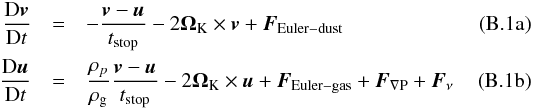 where v is the particle velocity and u the gas velocity, D / Dt is the material derivative, the first term on the RHS is the drag force, the second term is the Coriolis force, and FEuler = − (dΩK/ dt) × r is the Euler force that arises due to the radial motion. It therefore appears in the radial equations. In addition, the equation of motion for the gas includes a hydrostatic correction due to a radial pressure gradient (F∇P) and viscous forces (Fν). Following convention, we write the pressure gradient in terms of a nondimensional η:
  (B.2)and use the thin disk approximation (consider column densities Σgas instead of ρ) for the viscous force:
  (B.3)where T is the viscous stress tensor. In cylindrical coordinates, the only relevant term is:
  (B.4)with which the viscous force becomes
  (B.5)where ν is the kinematic viscosity. In the α-disk model we have that νΣgas is constant and therefore
 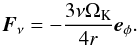 (B.6)In order to solve for the drift velocities, we put the accelerations on the LHS of Eq. (B.1) zero, Du/ Dt = Dv/ Dt = 0. This is justified, because a change in the drift velocities occurs on a timescale of ~r/vr, which is always much longer than the stopping time. Inserting Eqs. (B.2) and (B.6) into (B.1) gives a system of four equations and four unknowns (the velocities). Its solution is:
 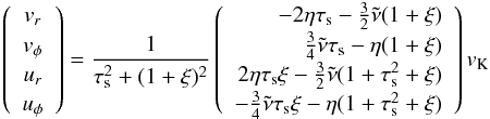 (B.7)where τs = tstopΩK, ξ = ρd/ρg, and
  . Note that in the α-prescription
  , that is, for α ≪ 1 the modification due to viscosity is minor.
Appendix C: Semi-analytical model
In this section we aim for an analytic prescription of the key characteristics of the steady-state ice and vapor distribution for any given disc model – not necessarily with the same gas and temperature profiles as assumed in this study. We will derive expressions for the peak of the ice surface density and its location, which enable us to determine whether the conditions for streaming instability beyond the snowline can be reached.
Appendix C.1: Location of the snowline
The location of the snowline, rsnow, is the outer-most radius where the entire incoming ice flux can thermodynamically exist in the gaseous state. Its location is found by equating the equilibrium (saturation) pressure to the vapor pressure of H2O corresponding to the incoming icy pebble flux, that is, Peq = PZ,a, where PZ,a is the steady-state vapor pressure; i.e., the vapor pressure obtained when all the H2O is in the gas phase. Therefore, the snowline rsnow is given by the radius r where ![Mathematical equation: \appendix \setcounter{section}{3} \begin{equation} P_\mathrm{eq,0} \exp \left[ -\frac{T_{\rm a}}{T(r)} \right] = \frac{k_{\rm B} T}{\mu} \frac{\Sigma_{Z,\mathrm{a}}}{\sqrt{2\pi}H_\mathrm{gas}} = \frac{k_{\rm B} T(r)}{\mu} \frac{\Mdotice/3\pi\nu(r)}{\sqrt{2\pi}H_\mathrm{gas}(r)} \label{eq:rsnow-eq} \end{equation}](/articles/aa/full_html/2017/06/aa30013-16/aa30013-16-eq271.png) (C.1)see Eqs. (11) and (34). Given Ṁice, α and a disk model, we can therefore readily solve (numerically) for rsnow.
(C.1)see Eqs. (11) and (34). Given Ṁice, α and a disk model, we can therefore readily solve (numerically) for rsnow.
A caveat of Eq. (C.1) is that the role of transport processes are neglected. These could potentially introduce disequilibrium corrections. However, we find that the times to achieve the equilibrium (saturation) pressure is typically much shorter than the transport timescales (by diffusion or drift).
Appendix C.2: The equilibrium density
Generalizing the above arguments to locations beyond rsnow, we approximate the vapor pressure with the saturation pressure – an approximation that is again justified as long as the timescales for evaporation (and condensation) are sufficiently short (in other words: the super-saturation level is small). Similarly, we can define a vapor surface density (Σeq) corresponding to Peq. Re-arranging Eq. (C.1) in terms of Σ we obtain this equilibrium surface density: ![Mathematical equation: \appendix \setcounter{section}{3} \begin{eqnarray} \nonumber \Sigma_\mathrm{eq} &\equiv& \frac{\sqrt{2\pi}H_\mathrm{gas} \mu}{k_{\rm B} T} P_\mathrm{eq} \\[5mm] &=& \Sigma_\mathrm{snow} \left( \frac{r}{r_\mathrm{snow}} \right)^p \exp\left[ \frac{T_{\rm a}}{T_\mathrm{snow}} \left(1 -\left( \frac{r}{r_\mathrm{snow}} \right)^q \right) \right] \label{eq:sigZ} \end{eqnarray}](/articles/aa/full_html/2017/06/aa30013-16/aa30013-16-eq275.png) (C.2)where Σsnow and Tsnow are the vapor surface density and the temperature at the location of the snowline. In Eq. (C.2) we have assumed power-laws for the temperature, gas surface density, and the gas scaleheight. In our case we have p = 7 / 4 and q = 1 / 2 (see Sect. 2.1).
(C.2)where Σsnow and Tsnow are the vapor surface density and the temperature at the location of the snowline. In Eq. (C.2) we have assumed power-laws for the temperature, gas surface density, and the gas scaleheight. In our case we have p = 7 / 4 and q = 1 / 2 (see Sect. 2.1).
Taylor-expanding the (weakly-varying) power-laws involved in the expression of Σeq around rsnow gives7: ![Mathematical equation: \appendix \setcounter{section}{3} \begin{equation} \Sigma_\mathrm{eq}(x) \approx \Sigma_\mathrm{snow} \left( 1 +px \right) \exp \left[ -\frac{qT_{\rm a}x}{T_\mathrm{snow}} \right] = \Sigma_\mathrm{snow} \left( 1 +px \right) {\rm e}^{ -a_\mathrm{eq} x} \label{eq:sigma-eq-approx} \end{equation}](/articles/aa/full_html/2017/06/aa30013-16/aa30013-16-eq280.png) (C.3)where x = (r − rsnow) /rsnow is the fractional distance beyond the snowline and
(C.3)where x = (r − rsnow) /rsnow is the fractional distance beyond the snowline and 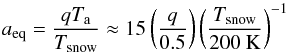 (C.4)is a dimensionless number that weakly depends on the location of the snowline.
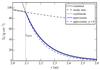 |
Fig. C.1 Vapor surface density profiles. Shown in black are the steady state vapor profile when all the ice is in the gas phase (thin solid curve), and the surface density corresponding to equilibrium vapor pressure Peq (Eq. (C.2); dashed solid curve). The snowline rsnow is located at the intersection of these two curves. The numerically-obtained profile (thick gray curve) closely follows the minimum of steady-state and equilibrium profiles. The blue curves present mathematically-convenient approximations to Σeq (see text), valid for r>rsnow. |
In Fig. C.1 the respective vapor density profiles have been plotted. Parameters correspond to those of the default model (Table 1). The simulated result of Sect. 4 is plotted by the thick gray curve. It is characterized by a sharp dent at rsnow. Exterior to the snowline ΣZ follows the equilibrium profile (solid black curve), while interior to rsnow, it is limited by the imposed mass flux (solid dashed curve). The approximate expressions derived in Eq. (C.3), valid for r>rsnow, are shown by the blue curves. We obtain rsnow = 2.09 au, Σsnow = 92 g cm-2 and aeq = 16.9. The solid blue curve approximates Σeq very closely. The dashed blue curves gives a further approximation to Σeq, obtained by putting p = 0. This slightly underestimates ΣZ but nevertheless gives a reasonable approximation that we will use below.
Assuming ΣZ = Σeq for the vapor density beyond rsnow, we write for the associated mass flux ℳZ:![Mathematical equation: \appendix \setcounter{section}{3} \begin{eqnarray} \mathcal{M}_Z \approx \mathcal{M}_{\mathrm{eq}} \nonumber &=& -v_\mathrm{gas}\Sigma_\mathrm{eq} -D_\mathrm{gas} \Sigma_\mathrm{gas} \frac{{\rm d}}{{\rm d} r} \left( \frac{\Sigma_\mathrm{eq}}{\Sigma_\mathrm{gas}} \right) \\[3mm] \label{eq:Mz-eq-def} &\approx& -v_\mathrm{gas}\Sigma_\mathrm{eq} -D_\mathrm{gas} \frac{{\rm d} \Sigma_\mathrm{eq}}{{\rm d} r} \end{eqnarray}](/articles/aa/full_html/2017/06/aa30013-16/aa30013-16-eq291.png) (C.5)where we neglected the curvature of the disk, i.e., we assumed that the scales over which Σeq and Σgas change are much smaller than r. This is justified as long as x ≪ 1. In a similar vein, we assume that quantites as Dgas and vgas do not vary. With Eq. (C.3) for Σeq we obtain:
(C.5)where we neglected the curvature of the disk, i.e., we assumed that the scales over which Σeq and Σgas change are much smaller than r. This is justified as long as x ≪ 1. In a similar vein, we assume that quantites as Dgas and vgas do not vary. With Eq. (C.3) for Σeq we obtain: ![Mathematical equation: \appendix \setcounter{section}{3} \begin{eqnarray} \label{eq:Mz-eq} \frac{\mathcal{M}_{\mathrm{eq}}}{D_\mathrm{gas}/r_\mathrm{snow}} &=& -\frac{v_\mathrm{gas}r_\mathrm{snow}}{D_\mathrm{gas}}\Sigma_\mathrm{eq}- \frac{{\rm d}\Sigma_\mathrm{eq}}{{\rm d}x} \\[3mm] \nonumber &=& \Sigma_\mathrm{snow}\left( -b_\mathrm{gas} (1+px) + a_\mathrm{eq}(1+px) -p \right) {\rm e}^{-a_\mathrm{eq}x} \\[3mm] &\approx& \Sigma_\mathrm{snow} (a_\mathrm{eq} -b_\mathrm{gas}) {\rm e}^{-a_\mathrm{eq} x} \end{eqnarray}](/articles/aa/full_html/2017/06/aa30013-16/aa30013-16-eq294.png) where bgas = vgasrsnow/Dgas is the dimensionless gas velocity and in the last step p = 0. In a viscously-evolving disk vgas = 3ν/ 2r and hence bgas = 1.5.
where bgas = vgasrsnow/Dgas is the dimensionless gas velocity and in the last step p = 0. In a viscously-evolving disk vgas = 3ν/ 2r and hence bgas = 1.5.
Appendix C.3: The ice profile
With the equilibrium profile as the approximation to the vapor density, we solve for the surface density of the ice by invoking conservation of mass. In steady-state the total H2O mass flux ℳtot,ice = ℳice + ℳZ is constant. Interior to the snowline, ℳZ = ℳtot,ice while for r ≫ rsnowℳZ ≪ ℳice ≈ ℳtot,ice. But near the snowline the mass fluxes change rapidly. Here, the steep gradient in the vapor density causes an outward (positive) mass flux, which increases the inwardly-directed icy pebble flux: 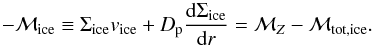 (C.8)(Note that just outside rsnow, ℳice and ℳtot,ice are negative and ℳZ is positive.) With ℳeq for ℳZ Eq. (C.8), in terms of x, reads
 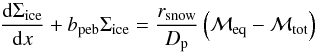 (C.9)where bpeb = rsnowvpeb/Dp is the ratio between the speed at which the pebbles drift in and the radial velocity of the gas. Usually, pebbles outpace the gas and bpeb ≫ 1.
To solve Eq. (C.9) we will assume that bpeb and other parameters are constant in x. Assuming constant bpeb is clearly an approximation, since the pebbles may (i) acquire thick icy mantles on their approach to the snowline but (ii) lose all their ice once their are very close to rsnow. Hence, the aerodynamical properties of the pebbles and therefore vpeb are expected to vary considerably. Disregarding these concerns, momentarily, the solution to Eq. (C.9) reads: ![Mathematical equation: \appendix \setcounter{section}{3} \begin{eqnarray} \Sigma_\mathrm{ice}\nonumber &= &{\rm e}^{-b_\mathrm{peb} x} \int_0^x {\rm e}^{b_\mathrm{peb} x'} \frac{r_\mathrm{snow} \mathcal{M}_{\mathrm{eq}}(x')}{D_{\rm{p}}} {\rm d}x' \\[3mm] &= &\Sigma_\mathrm{snow}(1-\epsilon_\mathrm{gas}) \left[ \frac{c_\mathcal{M}(1-{\rm e}^{-a_\mathrm{eq}\varepsilon x})}{\varepsilon} +\frac{{\rm e}^{-a_\mathrm{eq}x} -{\rm e}^{-a_\mathrm{eq}\varepsilon x}}{\varepsilon-1} \right] \label{eq:sigice-sol} \end{eqnarray}](/articles/aa/full_html/2017/06/aa30013-16/aa30013-16-eq310.png) (C.10)where we used Eq. (C.6) for ℳeq, put p = 08 and defined ε = bpeb/aeq, εgas = bgas/aeq and cℳ = − ℳtot,icersnow/ ΣsnowDp(aeq − bgas) to keep the notation concise. Typically, εgas ≈ 1.5 /aeq and cℳ are small numbers. In a steady-state viscous disk Σsnow ≈ Ṁice/ 2πrvgas and ℳtot,ice = − Ṁice/ 2πrsnow. Hence in a viscous disk cℳ is related to εgas:
(C.10)where we used Eq. (C.6) for ℳeq, put p = 08 and defined ε = bpeb/aeq, εgas = bgas/aeq and cℳ = − ℳtot,icersnow/ ΣsnowDp(aeq − bgas) to keep the notation concise. Typically, εgas ≈ 1.5 /aeq and cℳ are small numbers. In a steady-state viscous disk Σsnow ≈ Ṁice/ 2πrvgas and ℳtot,ice = − Ṁice/ 2πrsnow. Hence in a viscous disk cℳ is related to εgas:  (C.11)In Fig. C.2 we plot Σice for the parameters of the default model (Table 1). The simulated data are given by the thick grey curve while the analytical profiles are in blue – the more precise approximation (with p = 7 / 4; solid) and the p = 0 case in dashed. The analytical profiles fit the simulation data very well. The key parameter for the analytical profiles is the velocity of the pebbles vpeb. Here, we have chosen vpeb to be the pebble velocity at the ice peak rpeak, vpeb ≈ 2.4 m s-1, which provides a decent fit. The fit is somewhat sensitive to the choice of vpeb; for example, adopting vpeb(rpeak) with the initial value for mice (i.e., without deposition of vapor) would overestimate the numerical curve by 20%.
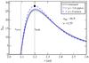 |
Fig. C.2 Steady state surface density of ice for the default model parameters. The simulated profile from the numerical model (thick grey line) is well reproduced by the full analytical solution using p = 7 / 4 (solid curve; formula not shown in the main text) and the further p = 0 approximation (dashed curve; Eq. (C.10)). The black square denotes the values corresponding to the mass peak (rpeak,Σpeak) given by Eqs. (C.12) and (C.13). |
Appendix C.4: Peak values and final tuning
Equation (C.10) has a maximum at (x,Σice) = (xpeak,Σpeak) where ![Mathematical equation: \appendix \setcounter{section}{3} \begin{equation} \label{eq:rpeak} x_\mathrm{peak} = \frac{\log \left[ \varepsilon +c_\mathcal{M}(\varepsilon-1)\right]}{a_\mathrm{eq}(\varepsilon-1)} \end{equation}](/articles/aa/full_html/2017/06/aa30013-16/aa30013-16-eq325.png) (C.12)or rpeak = (1 + xpeak)rsnow in dimensional units, and
(C.12)or rpeak = (1 + xpeak)rsnow in dimensional units, and ![Mathematical equation: \appendix \setcounter{section}{3} \begin{equation} \label{eq:sigpeak} \Sigma_\mathrm{peak} = (1-\varepsilon_\mathrm{gas}) \frac{c_\mathcal{M} +\left[ c_\mathcal{M}(\varepsilon-1) +\varepsilon\right]^{1/(1-\varepsilon)}}{\varepsilon} \Sigma_\mathrm{snow}. \end{equation}](/articles/aa/full_html/2017/06/aa30013-16/aa30013-16-eq327.png) (C.13)Since cℳ and εgas are fixed, the latter expression only depends on ε. Lower ε – meaning: a smaller pebble velocity at rpeak – increases both the width (xpeak) and the magnitude of the ice peak, resulting in a more pronounced, “fatter” ice bump.
(C.13)Since cℳ and εgas are fixed, the latter expression only depends on ε. Lower ε – meaning: a smaller pebble velocity at rpeak – increases both the width (xpeak) and the magnitude of the ice peak, resulting in a more pronounced, “fatter” ice bump.
All that remains is to find an expression for the pebble velocity at the ice peak vpeb, which in turn depends on the amount of ice those pebbles have accreted. To obtain mpeb = mcore + mice we invoke conservation of the pebble number flux  (C.14)Hence, we can obtain mice from Σpeak, calculate the aerodynamical properties of the pebbles at the peak (i.e., their stopping time) and obtain the pebble velocity vpeb.
With Eq. (C.14) we have a closed system of expressions to obtain the relevant quantities at the ice peak. These can best be computed by an iterative scheme, e.g.,
-
1.
From (an initial guess for) ε obtain Σpeak and the position of the ice peak rpeak from the ice flux conservation model, Eq. (C.13) .
-
From Σpeak, obtain the ice mass mice at the ice peak from the pebble conservation law, Eq. (C.14).
-
3.
From mice and the gas properties at r = rpeak, compute the stopping time of the pebbles at rpeak. Update the pebble velocity vpeb and its normalized variant ε.
This scheme can easily be extended with collective and mean molecular weight effects (i.e., the complete model). Finally, in order to obtain a better match to our numerical results we adopt two ad-hoc empirical “fixes”. First we reduce Eq. (C.13) by 10%, which accounts for the fact that the p = 0 approximation tends to overestimate the peak. Secondly, we slightly increase ε when it drops below unity. This fix approximately accounts for curvature effects (not included in the model) that become apparent when the ice peak becomes broad (at low ε). Hence we take ε = max(ε ∗ ,ε ∗ 0.8) where ϵ ∗ = (vpeb,peakrpeak/a2Dpeak) is the uncorrected value.
In Table C.1 a comparison of the model with the numerically-obtained peak parameters is given for a number of model parameters. Generally, the agreement is very good; the error in Σpeak is at most 20%. Given its crudeness, the analytical model, however, does not always produce a perfect match – especially not when it comes to the profile. For example the low turbulence runs (α = 3 × 10⁻⁴), which imply high gas densities when Ṁgas is kept the same, still show a good match to Σpeak, but the profile corresponding to Eq. (C.10) is very different from the numerical model. The reason for this is that pebbles enter the Stokes drag regime when approaching the ice peak, causing a sharp increase in the stopping time (and ε). The stopping time at the ice peak is in that case not representative for other radii.
Comparison between analytical and numerical model.
All Tables
All Figures
|
Fig. 1 Schematic showing the difference between the single-seed model and the many-seeds model for the internal structure of icy pebbles in the outer disk. In the single-seed model, the water ice layer (white) on the silicate core (red) becomes smaller at the evaporation front, and after complete evaporation of the ice, only one single silicate core remains. Since we take ζ = 0.5, the silicate core contains half the mass of the original pebble: mcore = mice = 0.5mp,start. In the many-seeds model, pebbles in the outer disk consist of many micron-sized silicate grains (red) “glued” together by water ice (white). As the ice evaporates, silicate grains are released as well. After complete evaporation of the ice, many micron-sized silicate grains remain. Again, with ζ = 0.5, the total mass in silicate grains in a pebble in the outer disk is half of the total pebble mass, but this mass is now divided among many silicate grains that each have mass msil. See text for more details. |
| In the text | |
|
Fig. 2 The solution to the transport equations at different points in time, for the fiducial model parameters listed in Table 1. At t = 105yr, approximately 90% of the steady-state peak in the ice surface density has formed. a) Surface densities Σ of ice (solid lines) and vapor (dashed lines). The dotted line corresponds to the steady-state advection-only vapor surface density profile. b) Midplane pebbles-to-gas ratio ρpeb/ρgas. c) Typical pebble mass mp. d) Typical pebble internal density ρ•,p. |
| In the text | |
|
Fig. 3 Rate of change of the ice surface density at the peak location, as function of time. The rate of change increases until the icy pebble front has reached the peak location, after which the peak continues to grow at an exponentially decreasing rate, while the system is converging to its steady-state solution. |
| In the text | |
|
Fig. 4 Steady-state results for the fiducial parameters, for the simple model with single-seed evaporation (upper two panels) and many-seeds evaporation (lower two panels). a) Surface densities of ice, silicates and vapor (Σice, Σsil, and ΣZ, respectively) for the single-seed model. The silicates are locked in the icy pebbles outside the snowline, whereas they are bare grains interior to the snowline. b) Midplane pebbles-to-gas ratio ρpeb/ρgas, and pebbles-to-gas column density ratio Σpeb/ Σgas for the single-seed model. c) Same as panel a) but for the many-seeds model. The silicates are now divided in two populations: silicates that are locked up in icy pebbles (Σdirt), and free silicates (Σsil). Note that in panels a) and c) the x-axis ranges between r = 1.8 − 2.8au, for clarity. d) Same as b), but for the many-seeds model and with an additional line for the midplane “free silicates”-to-gas ratio ρsil/ρgas. |
| In the text | |
|
Fig. 5 Comparison of steady-state results for the fiducial parameters between the simple model (dashed lines) and the complete model (solid lines), which includes collective effects and the effects of the variation of the mean molecular weight μ. The upper two panels correspond to the single-seed evaporation model; the lower two panels correspond to the many-seeds evaporation model. In the latter case, we made the conservative choice of not including the free silicates in the back-reaction onto the gas. a) Surface densities of ice (Σice), vapor (ΣZ) and silicates (Σsil) for the single-seed model. The grey line indicates the mean molecular weight of the gas in units of proton mass mH. b) Midplane pebbles-to-gas ratio ρpeb/ρgas. c) Same as a), but the silicates are now divided into “free silicates” (Σsil) and “locked silicates” (Σdirt). For clarity, we only show the clean Σice profile for comparison. d) Same as b), with an additional line denoting the “free silicates”-to-gas ratio ρsil/ρgas. |
| In the text | |
|
Fig. 6 Comparison of steady-state results for the simple, single-seed, fiducial model between the case where vapor has the same vertical distribution as the background gas (HZ = Hgas) and the case where vapor has the same scale height as the pebbles (HZ = Hpeb). In all three panels, solid lines correspond to the HZ = Hgas case and dashed lines correspond to the HZ = Hpeb case. a) Steady-state water ice (blue) and water vapor (green) surface densities. b) Midplane solids-to-gas ratios (green) and solids-to-gas surface densities ratios (blue). c) Typical pebble mass mp. |
| In the text | |
|
Fig. 7 a) Contours of constant relative ice surface density peak heights fΣ,peak (see text for details) as function of turbulence parameter α and solids-to-gas accretion rate ℱs / g. The gas accretion rate Ṁgas is fixed to 10-8M⊙yr-1 and the initial size of the pebbles τ3 is fixed to 0.03. b) Contours of constant relative ice surface density peak heights (see text for details) as function of the turbulence parameter α and the gas accretion rate Ṁgas. The solids-to-gas accretion rate ratio ℱs / g is fixed to 0.4 and the initial size of the pebbles τ3 is fixed to 0.03. The cyan lines denote a Toomre parameter (QT) of unity at 10 au (1 au); the space below these lines has QT< 1 and is gravitationally unstable at 10 au (1 au). |
| In the text | |
|
Fig. 8 a) Contours of midplane solids-to-gas ratios (black) as function of the turbulence parameter α and the solids-to-gas accretion rate ℱs / g. The gas accretion rate Ṁgas is fixed to 10-8M⊙yr-1 and the initial size of the pebbles τ3 is fixed to 0.03. Orange contours denote the amount of solid material (in Earth masses) that is required to form the eventual peak in the ice surface density just outside the snowline. b) Contours of midplane solids-to-gas ratios as function of α and Ṁgas. The solids-to-gas accretion rate ℱs / g is fixed to 0.4 and the initial size of the pebbles τ3 is fixed to 0.03. Orange contours denote the amount of solid material (in Earth masses) that is required to form the eventual peak in the ice surface density just outside the snowline. The cyan lines denote a Toomre parameter (QT) of unity at 10 au (1 au); the space below these lines has QT< 1 and is gravitationally unstable at 10 au (1 au). |
| In the text | |
|
Fig. 9 Peak midplane solids-to-gas ratio as function of τ3. Ṁgas is fixed at 10-8M⊙yr-1, ℱs / g at 0.4, and the value of α is 3 × 10⁻³. We can distinguish four regimes I–IV, which are explained in the main text. |
| In the text | |
|
Fig. C.1 Vapor surface density profiles. Shown in black are the steady state vapor profile when all the ice is in the gas phase (thin solid curve), and the surface density corresponding to equilibrium vapor pressure Peq (Eq. (C.2); dashed solid curve). The snowline rsnow is located at the intersection of these two curves. The numerically-obtained profile (thick gray curve) closely follows the minimum of steady-state and equilibrium profiles. The blue curves present mathematically-convenient approximations to Σeq (see text), valid for r>rsnow. |
| In the text | |
|
Fig. C.2 Steady state surface density of ice for the default model parameters. The simulated profile from the numerical model (thick grey line) is well reproduced by the full analytical solution using p = 7 / 4 (solid curve; formula not shown in the main text) and the further p = 0 approximation (dashed curve; Eq. (C.10)). The black square denotes the values corresponding to the mass peak (rpeak,Σpeak) given by Eqs. (C.12) and (C.13). |
| In the text | |
Current usage metrics show cumulative count of Article Views (full-text article views including HTML views, PDF and ePub downloads, according to the available data) and Abstracts Views on Vision4Press platform.
Data correspond to usage on the plateform after 2015. The current usage metrics is available 48-96 hours after online publication and is updated daily on week days.
Initial download of the metrics may take a while.