| Issue |
A&A
Volume 601, May 2017
|
|
|---|---|---|
| Article Number | A135 | |
| Number of page(s) | 12 | |
| Section | The Sun | |
| DOI | https://doi.org/10.1051/0004-6361/201630082 | |
| Published online | 23 May 2017 | |
Vortex flows in the solar chromosphere
I. Automatic detection method
Institute of Theoretical Astrophysics, University of Oslo, PO Box 1029 Blindern, 0315, Oslo, Norway
e-mail: This email address is being protected from spambots. You need JavaScript enabled to view it.
;
e-mail: This email address is being protected from spambots. You need JavaScript enabled to view it.
Received: 17 November 2016
Accepted: 18 February 2017
Abstract
Solar “magnetic tornadoes” are produced by rotating magnetic field structures that extend from the upper convection zone and the photosphere to the corona of the Sun. Recent studies show that these kinds of rotating features are an integral part of atmospheric dynamics and occur on a large range of spatial scales. A systematic statistical study of magnetic tornadoes is a necessary next step towards understanding their formation and their role in mass and energy transport in the solar atmosphere. For this purpose, we develop a new automatic detection method for chromospheric swirls, meaning the observable signature of solar tornadoes or, more generally, chromospheric vortex flows and rotating motions. Unlike existing studies that rely on visual inspections, our new method combines a line integral convolution (LIC) imaging technique and a scalar quantity that represents a vortex flow on a two-dimensional plane. We have tested two detection algorithms, based on the enhanced vorticity and vorticity strength quantities, by applying them to three-dimensional numerical simulations of the solar atmosphere with CO5BOLD. We conclude that the vorticity strength method is superior compared to the enhanced vorticity method in all aspects. Applying the method to a numerical simulation of the solar atmosphere reveals very abundant small-scale, short-lived chromospheric vortex flows that have not been found previously by visual inspection.
Key words: Sun: atmosphere / Sun: chromosphere / Sun: magnetic fields
© ESO, 2017
1. Introduction
A solar “magnetic tornado” is generated when the footpoint of a magnetic field structure coincides with an intergranular vortex flow in the photosphere and topmost parts of the convection zone (Wedemeyer & Steiner 2014). The rotation is mediated by the magnetic field into the chromosphere, where the plasma is forced to follow the rotating magnetic field and thus creates an observable vortex flow that is referred to as “chromospheric swirl” (Wedemeyer-Böhm & Rouppe van der Voort 2009). A small-scale quiet Sun vortex is also observed by Park et al. (2016) in different chromospheric spectral lines. Solar tornadoes extend farther into the corona above and thus provide channels for the transfer of magneto-convective mechanical energy into the upper solar atmosphere, thus making them a potential candidate for contributing to the heating of the chromosphere and corona. Wedemeyer-Böhm et al. (2012) find that, based on numerical simulations, a sufficient amount of Poynting flux could be carried upwards in a magnetic tornado. A more detailed determination of the net energy flux, which is in principle provided in the upper solar atmosphere, requires a systematic statistical analysis of the properties of solar tornadoes. Previous studies relied on visual inspections of chromospheric observations, mostly in the Ca II infrared triplet line at 854.2 nm, and produced somewhat small sample sizes. For instance, Wedemeyer-Böhm et al. (2012) detected 14 swirls within a field of view of 55′′ × 55′′ during an observation with a duration of 55 min, implying a occurrence of 1.9 × 10⁻⁴ vortices Mm-2 min-1 and an average lifetime of (12.7 ± 4.0) min. The occurrence rate of chromospheric vortex flows seems to be roughly one order of magnitude smaller than the corresponding rate for photospheric vortices of 3.1 × 10⁻³ vortices Mm-2 min-1 found by Bonet et al. (2010). A lower occurrence of chromospheric vortices is expected to some extent when assuming that the formation of a chromospheric vortex requires both a driving photospheric vortex and a co-located magnetic field structure (Wedemeyer & Steiner 2014). However, given the challenges with reliably spotting chromospheric swirls as part of the complex dynamics exhibited in such observational image sequences, the derived occurrence rate has to be considered a rough estimate and most likely a lower limit only. Apart from the unknown effect of yet undetected vortex flows on the transport of energy and mass, more accurate occurrence rates of vortex flows could help to characterise the nature of turbulent flows in the solar atmosphere.
In this first paper of a series, we describe an automatic detection method that is capable of identifying the observable signatures of magnetic tornadoes in complex flow patterns, which is a necessary next step towards a quantitative determination of the possible contribution of magnetic tornadoes to the heating of the upper solar atmosphere. The method was developed and tested with numerical simulations produced with CO5BOLD (Freytag et al. 2012). After the description of the method in Sect. 2, which combines line integral convolution (LIC) imaging techniques, vorticity, and vorticity strength, we demonstrate the results for one of the CO5BOLD simulations in Sect. 3. After a discussion of the results in Sect. 4, conclusions and an outlook are provided in Sect. 5. In forthcoming papers of this series, the full analysis results for a sequence of numerical simulations and for observational data sets will be presented.
2. Method
The method presented here consists of the following steps: determination of the velocity field (Sect. 2.1); vortex detection (Sect. 2.4) based on vorticity and vorticity strength (Sect. 2.3); and event identification (Sect. 2.5). In Appendix A, we show the flowchart of our method step-by-step. The method is tested and illustrated first with a very simplified vortex flow (Sect. 2.2) and then with a more realistic combination of a numerical model atmospheres and a fixed vortex flow (Sect. 2.6).
2.1. Determination of the velocity field
Quantitative studies of atmospheric dynamics (e.g. November 1986; November & Simon 1988) require that the velocity field in the solar atmosphere is known with sufficient accuracy. Unfortunately, the large degree of dynamics, which occurs on a large range of temporal and spatial scales, make the reliable determination of the atmospheric velocity field from observations a challenging task. Alongside the complexity of multidimensional flows in the solar atmosphere itself, observational effects such as intermediate blurring as a result of varying seeing conditions, and limited spatial resolution make it difficult to find swirling features. Some of the difficulties can be overcome by advanced feature-tracking techniques such as the commonly known local correlation tracking (LCT). For instance, the FLCT method by Welsch et al. (2004) and Fisher & Welsch (2008) is able to determine the velocity field from sequences of observational images with sufficient quality.
Nevertheless, how well the derived LCT velocities match the actual physical velocities has to be thoroughly checked. Such tests can be performed on the basis of numerical simulations for which the initial physical velocities are known and can be compared to corresponding LCT velocites derived from synthetic observations of the simulated atmospheric dynamics. In this first paper of a series, however, we present a precursory step for which we use one of the model atmospheres created with CO5BOLD (Sect. 2.2) for testing our detection methods as described below. In future parts of this series, velocities derived with the FLCT method will be used and the implications of the inherently-limited velocity accuracy on the detection of vortex flows will be discussed.
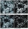 |
Fig. 1 Sample images illustrating the velocity distribution of a snapshot in our simulation (8 Mm × 8 Mm). a) LIC imaging scaled by the horizontal velocity amplitude, b) vorticity, c) LIC imaging scaled by the vorticity amplitude, and d) vorticity strength. Arrows indicate the velocity field. |
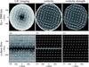 |
Fig. 2 Comparison between LIC imaging, vorticity, and vorticity strength of a solid rotation (upper panels) and that of a shear flow (lower panels) indicated by white arrows. Upper panels: a) the horizontal velocity amplitude of a swirling feature is illustrated by the LIC imaging, b) the tangential discontinuity at the edge of a swirling feature is enhanced by the vorticity, and c) the constant angular rotation speed of a swirling feature is depicted by the vorticity strength. Lower panels: d) same as a) but for a shear flow, e) a gap between the rightward and leftward velocity at y = 0 is illustrated by the vorticity, and f) there are no features shown by the vorticity strength. |
2.2. Model atmosphere for testing
The model was computed with the three-dimensional (3D) radiation magnetohydrodynamic code CO5BOLD (Freytag et al. 2012) and is equivalent to the one used by Wedemeyer-Böhm et al. (2012). However, it was produced with an improved numerical integration scheme (Steiner et al. 2013), resulting in reduced numerical diffusivity and thus more structure on smaller spatial scales. The new model was constructed by superimposing an initial magnetic field on a snapshot of a hydrodynamic simulation and advancing it in time until it had relaxed from this initial condition. The initial magnetic field was strictly vertical and had a field strength of | B0 | = 50 G.
The computational box comprised 286 × 286 × 286 grid cells and had a horizontal extent of 8.0 Mm × 8.0 Mm with a constant grid cell width of Δx = Δy = 28 km. The grid was non-equidistant in height and extended from −2.4 Mm at the bottom, in the convection zone, to 2.0 Mm at the top, in the model chromosphere, with a constant vertical grid spacing of Δz = 12 km at all z> − 128 km that gradually increased to Δz = 28.2 km for all z< − 1132 km.
The computational time steps were typically on the order of a few milliseconds. A sequence with a duration of 60 min and a cadence of 1 s was produced, of which the first 30 min were used for the tests presented in this paper.
2.3. Identification of vortices
An objective definition of a vortex has yet to be established and therefore the identification of vortices in complex or turbulent flows has been a primary subject (e.g. Jeong & Hussain 1995, and references therein). The so-called line integral convolution (LIC) technique turns out to be helpful in this respect. The LIC technique allows us to visualise turbulent flows and was first introduced by Cabral & Leedom (1993). A LIC image for a given velocity field is created by tracing streamlines whose intensity is proportional to the horizontal velocity amplitude. This technique can enhance the flow pattern of small-scale and large-scale eddies simultaneously, as can be seen in Fig. 1a, and therefore it can help to identify vortices by visual and automatic inspection. However, an automatic detection algorithm for vortices requires quantities that enables the objective, robust, and reproducible identification of vortices.
A vortex flow is by definition associated with a high value of the “vorticity” ω, which is defined as  (1)Unfortunately, the definition of the vorticity in Eq. (1) also results in high values for shear flows, meaning flows with opposite direction, which thus have to be distinguished from the sought-after true circular vortex flows. This ambiguity can be avoided by using the “vorticity strength” instead, which is the imaginary part of the eigenvalues of the velocity gradient tensor. The vorticity strength has indeed been successfully used by Moll et al. (2011) for investigating flow patterns in the surface-near layers of the convection zone and the photosphere. In our study, we use the same technique to investigate flow patterns in the chromosphere. In the following, we briefly demonstrate how the vorticity strength is used for finding swirling features in flows projected on a two-dimensional view plane.
Consider the velocity gradient tensor, 
 (2)If λ are the eigenvalues of , then
  (3)where I is the second order unit tensor. The eigenvalues can be determined by solving the characteristic equation
 ![Mathematical equation: \begin{equation} \det{\left[\mathcal{D}_{ij} - \lambda I\right]} =0 \label{eqn:determinant_tensor} \end{equation}](/articles/aa/full_html/2017/05/aa30082-16/aa30082-16-eq26.png) (4)which, for a velocity flow in two-dimensional space v = (vx,vy), can be written as
(4)which, for a velocity flow in two-dimensional space v = (vx,vy), can be written as  (5)where
  and
and  . Equation (5) has the following canonical solutions:
  (6)These solutions contain (i) one real root; (ii) two distinctive real roots; or (iii) a conjugate pair of complex roots. In general, positive and negative signs of the real part of the solutions, Re(λ), indicate diverging and converging flows, respectively. The imaginary part of the solutions, Im(λ), indicates the strength of the angular rotation speed of a circular motion. For a complete description in terms of eigenvalues and eigenvectors of the velocity gradient tensor, see Chong et al. (1990) for all possible cases of flow field geometries in three-dimensional space.
As an example, we consider a circular flow centred at the origin, (x,y) = (0,0), with two components: (i) a constant angular rotation frequency ν in the counter-clockwise direction, and (ii) a radial flow with a constant velocity μ directed outwards away from the origin. First, the velocity is transformed from polar coordinates to Cartesian coordinates:![Mathematical equation: \begin{equation} \left[\begin{array}{c} v_{\rm x} \\ v_{\rm y} \end{array}\right]= \left[\begin{array}{lr} \cos{\theta} & -\sin{\theta} \\ \sin{\theta} & \cos{\theta} \end{array}\right] \left[\begin{array}{c} v_{\rm r} \\ v_{\rm \theta} \end{array}\right], \end{equation}](/articles/aa/full_html/2017/05/aa30082-16/aa30082-16-eq37.png) (7)where vr = μ, vθ = rν, and
(7)where vr = μ, vθ = rν, and  is the distance from the origin. The velocity vector can be represented as
 ![Mathematical equation: \begin{equation} {\boldsymbol v}=\left[\mu\left(\frac{x}{r}\right) -\nu y\right]{\boldsymbol e}_{\rm x} + \left[\mu\left(\frac{y}{r}\right) + \nu x\right]{\boldsymbol e}_{\rm y}. \end{equation}](/articles/aa/full_html/2017/05/aa30082-16/aa30082-16-eq41.png) (8)The velocity gradient tensor of this case can be represented as
(8)The velocity gradient tensor of this case can be represented as ![Mathematical equation: \begin{equation} \mathcal{D}_{\rm ij}=\left[\begin{array}{lr} \mu\left(\frac{x}{r^2}\right) & -\nu \\ \nu & \mu\left(\frac{y}{r^2}\right) \end{array}\right], \end{equation}](/articles/aa/full_html/2017/05/aa30082-16/aa30082-16-eq42.png) (9)which results in
(9)which results in  (10)and
 (11)(Eq. (5)). For a pure circular flow with μ = 0 and ν ≠ 0, the solution consists of a conjugate pair of complex roots of λ = ± iν. In contrast, for a radial, non-circular flow with μ ≠ 0 and ν = 0, the solution has two distinctive real roots of λ = μx/r2 and λ = μy/r2.
2.4. Vortex detection
Once the velocity field is provided, the vorticity and the vorticity strength are calculated according to Eqs. (1)–(6). The vorticity in a chromospheric layer in the simulations exhibits a complicated filamentary structure as shown in Fig. 1b. Prior to the detection procedure, the LIC technique is applied to the resulting sequence of vorticity maps to smooth and to enhance not only eddies but also circular flows so that they become easier to detect (Fig. 1c). This preparatory step has proven to reduce the computational costs of the vortex detection procedure. In contrast, the corresponding vorticity strength map is composed of more isolated features, as shown in Fig. 1d, because it is sensitive to other aspects of the input velocity field beyond the pure vorticity1. The determination of vorticity and thus the detection of vortex flows is therefore ultimately limited by the spatial resolution and accuracy of the input velocity field.
In the following, we present tests for both the enhanced vorticity and vorticity strength methods. In both cases, one snapshot after another is processed sequentially. Potential vortex candidates are then found from the local maxima in the input map in the current snapshot. Next, a Gaussian kernel is fitted to the map around each vortex candidate, although a more sophisticated kernel function could be used in the future. The fitted Gaussian is then subtracted from the original map. A new iteration follows in which the resulting map is again searched for local maxima, the new vortex candidates are fitted, and the fitted Gaussians are again subtracted. This iterative process is repeated until the peak falls below a threshold value of 10% of the maximum peak in the original map. This procedure is similar to the CLEAN algorithm as used for interferometric imaging (Högbom 1974) for the purpose of excluding irregular features and artefacts. The size of a vortex is determined approximately as the diameter of a circle whose area is equivalent to the area enclosed by a contour line for intensity values larger than 10% of the intensity peak value.
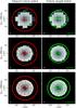 |
Fig. 3 Examples of the detection procedure for a vortex with a solid body rotation by using the enhanced vorticity method (left column) and the vorticity strength method (right column). The diameter of the rotating feature D0 is 200 km for a) and b), 400 km for c) and d), and 1000 km for e) and f), respectively. LIC imagings are shown in grey-scale in the background. Red and green crosses and circles indicate the location and the size of detected vortices, respectively. Thick crosses and circles mark the detections in the first iteration. |
The results from a detection based on the enhanced vorticity and another detection based on the vorticity strength were compared to determine which of the quantities produces the most reliable and complete outcomes. Figure 2 shows the difference between the LIC image, the vorticity, and the vorticity strength for a velocity field given by a solid rotation (upper panels) and by a shear flow (lower panels). The intensity of the LIC image is proportional to the horizontal velocity amplitude and thus shows a hollow structure that is higher in the outer parts of the tested flow patterns (panels (a) and (d)). Distinguishing between vortex flow and shear flow thus requires us to take into account the entire flow structure. This requirement is problematic for a more realistic velocity field (Fig. 1a), in which the boundaries between individual vortex flows can be difficult to see. Uncertainties in the velocity map derived from observations could severely limit the detection of vortices when using LIC imaging only.
Both the vorticity and vorticity strength have a much stronger signature, which thus results in a more robust detection method. The vorticity has large values for tangential discontinuities as found at the boundary between a rotational flow and the background, as shown in Fig. 2b. Therefore, areas of high vorticity are outlining the boundary, and thus the area, of a vortex flow instead of the location of the centre of a vortex flow. The vorticity strength, on the other hand, has the advantage that it can clearly discriminate between a solid rotation and a shear flow, as can seen from comparing panels (c) and (f) in Fig. 2.
Figure 3 shows how our methods detect a swirling feature with different diameters of D0 = 200 km for panels (a) and (b), D0 = 400 km for (c) and (d), and D0 = 1000 km for (e) and (f). The enhanced vorticity method and the vorticity strength method both successfully detect the smallest swirling feature in panels (a) and (b) but return significantly different sizes. The size of the isolated swirling feature measured by the enhanced vorticity method is larger than its actual size whereas the vorticity strength method produces more accurate results. The main reason for this difference is that the vorticity is sensitive to the tangential discontinuity at the edge of a swirling feature, as already shown in Fig. 2b, whereas the vorticity strength is not sensitive to the discontinuity. For the larger swirling features in panels c–f, on the other hand, both methods tend to detect multiple features within the same vortex flows. The sizes measured by both methods are similar but larger than the actual size of the vortex flow. The multiple detections are found in further iterations due to residues remaining after subtracting a fitted feature with a Gaussian kernel from the actual feature that has a sharp edge. The areas of the multiple small-size detections often overlap and can be combined into one detection that correctly represents the given vortex flow. In this particular simple and clear test case, the small vortex candidates even coincide with the large candidate detected in the first iteration and are therefore unnecessary. These unwanted, artificial detections are removed by post-processing in each frame.
2.5. Event identification
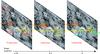 |
Fig. 4 Schematic illustration of how the detected features (red crosses in circles) are attributed to the same events in an image sequence. Orange, yellow, light-blue, and green circles indicate the identified events 1, 2, 16, and 17. The orange and yellow dashed lines illustrate the characteristic cone corresponding to a fixed characteristic speed (e.g. either the sound speed or the Aflvén speed). We choose to scan ten timesteps backwards to check the connectivity between the detected features and to confirm that they belong to the same event as illustrated for event 2. Involving several timesteps is important in case the event is not properly, or not all, detected in an intermediate timestep. In case of multiple detection candidates for the connectivity (e.g. multiple detections within a yellow dashed circle), we select the candidate being closest in terms of location and size. |
The previous steps return a number of consolidated vortex detections for each snapshot of the input image sequence. In this last step, detections from consecutive snapshots are combined into actual vortex events. The procedure is illustrated in Fig. 4. To decide if detected features belong to the same event or not, the geometrical distance between the features in the different snapshots must be less than the distance according to both a set maximum speed and the time difference between the analysed snapshots. Here, the maximum speed was set to 50 km s-1 which was the maximum Alfvén speed occurring in the simulation. Any larger distance would then imply that the difference in position of two detections is not physical and that these detections are not connected. We chose to scan ten timesteps backwards (approximately 10 s in this case) to check the connectivity of the detected features. In cases of multiple candidates within the limiting distance, the detection was chosen that led to the smallest change in size between the two detected features. The procedure could be replaced with a more sophisticated method using the cross-correlation function in a future upgrade.
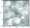 |
Fig. 5 LIC imaging averaged over the sampled time period of 30 min in the simulation. The location of the test vortices are indicated by a black cross at (x, y) = (0, 0) and black circles with diameters of D0 = 200 km, 400 km, and 1000 km, respectively. The strong magnetic field region is indicated by a dashed contour line enclosing the region in which the time-averaged magnetic field strength is larger than the initial magnetic field strength of 50 G. |
2.6. Tests with more realistic flow fields
In the previous sections, we showed that both the enhanced vorticity method and the vorticity strength method can detect an isolated vortex flow with a solid body rotation. However, typical flow fields in the solar atmosphere are much more complicated and the successful detection of vortex flows is much more challenging task. To demonstrate how our method works for more realistic flow fields in the solar atmosphere, we added a steady vortex with a solid body rotation to our realistic model atmosphere. This combination has the advantage that the properties of the vortex flow are well-known but that the fluctuations of the background are more realistic.
Figure 5 shows the time-average of the LIC images over the time period of 30 min. The time-averaged LIC image corresponds well to the magnetic field distribution. A steady vortex flow was added as a reference case in the central region at (x,y) = (0,0), where there are relatively few significant features otherwise. As in the simplified test case used before, a vortex flow with solid body rotation and a fixed diameter D0 was used as a reference case. Three different diameters of D0 = 200, 400, and 1000 km were tested for the reference vortex. The detection of the added vortex flow may depend on the interference from the nearby swirling features and the background, which may affect the resulting lifetime and the size of the artificial test vortex.
Performance results for the enhanced vorticity and the vorticity strength method based on tests with artificial vortex flows superimposed on a “realistic” simulated flow field.
As a measure for the success of the detection method, we estimated the detection rate of the test vortex as the ratio of the number of frames with a successful detection, n, and the total number of frames N during the simulation time of T = 30 min:  (12)We also measured the offset distance di of the detected test vortex from the original position in each frame, i, and obtained the mean offset distance
  :
:  (13)We then evaluated the position accuracy as the ratio between the mean offset distance and the original radius of the test vortex r0 ≡ D0/ 2:
 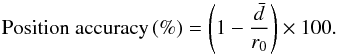 (14)The deviation σ of the diameter of a test vortex Di in each frame, as derived with the detection algorithm from the original diameter of the test vortex D0, is given by
 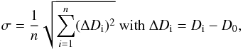 (15)and the mean error
  in the returned vortex diameter is
  (16)The relative accuracy in the detected size can then be expressed as
 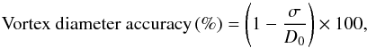 (17)with a size ratio of 100% representing a perfect result. The results are summarised in Table 1.
Based on this test, the vorticity strength method turns out to be superior to the enhanced vorticity method. The detection rate of the vorticity strength method is 99.9% independent of the size of the test vortex and thus higher than the corresponding rate for the enhanced vorticity method, which varies with vortex size but is 95.0% at best (Table 1). The position accuracy of the vorticity strength method is more than 95% but varies slightly, depending on the size of the test vortex. At the same time, the method always overestimates the actual size of the test vortex, resulting in a size accuracy between 60% and 80%. These results are nevertheless better than for the enhanced vorticity method as described below.
The enhanced vorticity method has a smaller rate of successful detections ranging from 70–95%, depending on the size of the to-be-detected test vortex. Furthermore, the positions and sizes returned by the enhanced vorticity method are less accurate than for the vorticity strength method. It is important to emphasise that the test cases in Fig. 3 have very sharp edges, whereas the transition between the vortices and the background flow field in the more realistic test case is much smoother. The enhanced vorticity method contains the convolution of streamlines and vorticity maps, which effectively results in the smoothing of gradients. Although this degrading effect still leaves clear enough boundaries in the test case with isolated vortices, these boundaries become very unclear for the test case with a more realistic background, resulting in low performance of the enhanced vorticity method. The vorticity strength approach, on the other hand, is able to detect the actual size of the swirling features without any problems because the method does not involve convolution with streamlines and thus no degrading of the vorticity strength maps. The method therefore performs much better for both types of test cases.
3. Results
In the following, we present the results for all vortex flows detected in 30 min long simulation sequence (Sect. 2.2).
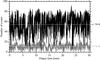 |
Fig. 6 Number of events detected with the vorticity strength method (grey curve) and with the enhanced vorticity method (black curve). The time-averaged numbers of events detected with the vorticity strength and the enhanced vorticity methods are 54.6 and 11.4, respectively. |
3.1. Number of events
The total numbers of events found with the enhanced vorticity method and the vorticity strength method are 1720 and 1600, respectively, and hence the occurrence rates of events are 8.9 × 10⁻¹ vortices Mm-2 min-1 and 8.3 × 10⁻¹ vortices Mm-2 min-1, respectively. Although these numbers are very similar, the number of events in each time step, meaning the instantaneous vortex detections, are very different. The difference becomes obvious when plotting the number of events as a function of time (Fig. 6). For both methods, the numbers vary strongly in time. On average, the vorticity strength method detects approximately 55 vortices in each time step compared to only approximately 11 vortices per time step with the enhanced vorticity method. The enhanced vorticity method detects fewer events with shorter lifetime compared to the vorticity strength method, but then combines a larger number of them into the same events to result in a comparable overall numbers of events.
3.2. Lifetime of swirling features
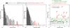 |
Fig. 7 Histograms of a) the lifetime of the detected events and b) the maximum diameter of the detected events. In panel c), the lifetime is plotted versus vortex diameter. In panels a) and b), the results found with the enhanced vorticity method are plotted with grey bars, whereas results of the vorticity strength method are shown as black lines. For comparison, the chromospheric swirls found by Wedemeyer-Böhm et al. (2012) are plotted with red lines. In panel c, all events detected in the simulation are grouped according to their lifetime in bins of 1 min. For each group, the average value is plotted as a horizontal line ± one standard deviation, indicated by the shorter horizontal line above and below. The maximum values are plotted as diamonds. Again, the results of the enhanced vorticity method are plotted in grey, whereas the results of the vorticity strength method are shown in black. For comparison, the chromospheric swirls observed by Wedemeyer-Böhm et al. (2012) are plotted as red diamonds with numbers according to the table in the supplementary information of their study. In addition, the clearest swirl described by Wedemeyer-Böhm & Rouppe van der Voort (2009) is represented as a green diamond, whereas the range of swirl diameters found in that study is marked as a green shaded area. |
In Fig. 7a, histograms for event lifetimes are shown as derived with the enhanced vorticity method and the vorticity strength method. For the enhanced vorticity method, the mean lifetime of the events is 16.0 s with a the standard deviation of 26.5 s, whereas the vorticity strength method produces events with a mean lifetime of 52.0 s and a standard deviation of 113 s. The events detected by the enhanced vorticity method last not more than 5 min, whereas the vorticity strength method results in a significant number of events with lifetimes of more than that. There is a particular event found by the vorticity strength method that seems to last 22 min. This particular case is due to clusters of swirling features that appear very close to each other. It is therefore not straightforward, in particular for an automated detection algorithm, to decide if an event persists as a single entity or if it is instead an intricate succession of splitting and merging vortices. Furthermore, this somewhat extreme lifetime exceeds the current longest reported lifetime for a chromospheric swirl of 19 min in the sample presented by Wedemeyer-Böhm et al. (2012). These kinds of extreme events must thus be considered with some caution although they are somewhat rare. It might be possible to further split these kinds of events into sub-events by using a cross-correlation function, but more detailed investigations leading to a more precise definition of vortex events would be needed.
3.3. Size of swirling features
Figure 7b shows histograms of the maximum diameter of vortex events detected by using both the enhanced vorticity method and the vorticity strength method. There are significant differences between them. The enhanced vorticity method results in a mean diameter of 533 km with a standard deviation of 274 km, whereas the vorticity strength method produces a mean radius of 338 km with a standard deviation of 132 km. As we describe in Sect. 2.6, the effective diameters measured by the enhanced vorticity method tend to be larger than those measured by the vorticity strength method. The number of events detected by the enhanced vorticity method drops sharply for diameters > 2000 km. The maximum diameter of the events detected by the enhanced vorticity method is 2215 km whereas that detected by the vorticity strength is 1449 km. Although the chromospheric swirls observed by Wedemeyer-Böhm et al. (2012) have diameters on average of 2.9 ± 1.0 Mm with the smallest value being 1.5 Mm, almost all events detected in our study are smaller than 2 Mm.
3.4. Correlation between lifetime and size
In Fig. 7c, the joint probability distribution for the lifetime and the size of detected events is compared to the observations of chromospheric swirls by Wedemeyer-Böhm et al. (2012). It seems that the sizes of the events detected in our simulation are distinctively different from the those of the observed chromospheric swirls, as we already mentioned in Sect. 3.3. Furthermore, there is no obvious relation between size and lifetime based on the current simulation-based sample. There is nevertheless some indication that the lifetimes and sizes correlate. This finding needs a more systematic analysis and will be addressed in a forthcoming publication.
4. Discussion
4.1. Occurrence rate of vortex flows
The occurrence rate of vortices is a quantitative indicator of the complexity of flows in the solar atmosphere. The event occurrence rates produced by the enhanced vorticity method and the vorticity strength method are both close to a value of 1 vortex Mm-2 min-1 (Sect. 3.1), which implies that a chromospheric vortex flow could exist for every granular cell. On the other hand, the value is four orders of magnitude larger than the value derived from observations of chromospheric swirls (e.g. Wedemeyer-Böhm et al. 2012) and three orders of magnitude larger than the value derived from observations of photospheric vortices (e.g. Bonet et al. 2010). This apparent discrepancy can be explained to a large extent by the limitations of observations as compared to the simulation analysed here. As can be seen in Fig. 7, there is a large number of small-scale and short-lived chromospheric vortex flows in the simulation. Those events have a mean lifetime in the range of 10 − 200 s (Sect. 3.2) and a mean diameter of roughly 400 km corresponding to ~ 0.5 arcsec. In comparison, Wedemeyer-Böhm & Rouppe van der Voort (2009) observed events with radii down to 0.4–0.6 arcsec and thus diameters on the order of 600–900 km, although a reliable analysis of such small events is already at the limit and most of their results are based on larger examples with diameters of up to ~ 2200 km (Fig. 7c).
4.2. Observational limitations
The successful detection of a vortex flow in an observational image sequence is a challenging task, which can be summarised with the following requirements:
-
The sub-structure of the vortex swirl, for example a ring, must beresolved clearly. Wedemeyer-Böhm &Rouppe van der Voort (2009) report ring widths ofonly 0.2 arcsec, which is close to the angular resolution that can typically be achieved with current solar telescopes. The width of the rotating ring described by Wedemeyer-Böhm & Rouppe van der Voort (2009) is about 10% of the swirl diameter. Scaling these proportions to a vortex diameter of only ~ 0.5 arcsec would imply ring widths of only 0.05 arcsec, which are clearly beyond what can be currently resolved.
-
The cadence of observation must be high enough that the plasma motions can be tracked reliably. Wedemeyer-Böhm & Rouppe van der Voort (2009) estimate horizontal speeds on the order of 10 km s-1. A feature rotating as part of a chromospheric vortex with that speed would move about 0.1 arcsec within roughly 7 s. A temporal resolution on that order or better is thus needed.
-
A rotating motion should be visible in a number of consecutive frames. Chromospheric observations often have cadences of 10 s or more. Detecting vortex flows with lifetimes of only a few 10 s is thus at the limit, in particular because rotating motions can easily be obscured by the generally complex dynamic pattern of the chromosphere. Reliable detections would thus favour longer-lived vortex events with at least one clear rotation cycle.
-
Variations in seeing conditions may make some frames less clear and thus reduce the overall effective cadence of the image sequence and thus the detectability of a vortex flow.
These requirements naturally result in limits for the shortest lifetimes and smallest diameters of vortex flows that can be reliably observed. The abundant small-scale events found in this paper would therefore remain undetected with current solar telescopes but pose an interesting science use case for the next generation of solar telescopes such as Daniel K. Inouye Solar Telescope (DKIST, formerly the Advanced Technology Solar Telescope, ATST, Keil et al. 2011) and the 4 m European Solar Telescope (EST, Collados et al. 2010)
4.3. Large-scale vortex flows
For the comparison with observations, we selected all detected events with diameters larger than 1000 km. The number of large-scale events is plotted as a function of simulation time in Fig. 8. The occurrence rates of large-scale events found with the enhanced vorticity method and the vorticity strength method are 7.1 × 10⁻² vortices Mm-2 min-1 and 8.8 × 10⁻³ vortices Mm-2 min-1, respectively. The latter is similar to the occurrence rate of observed photospheric vortices. This finding supports the conclusion that the discrepancy between the simulation results presented here and previous observations may, to a large extent, result from small-scale events that are undetected due to the lack of spatial or temporal resolution in observations.
For the large-scale events (i.e. with diameters > 1000 km) found with the enhanced vorticity method, the mean lifetime is 42.7 s and the maximum lifetime is 214 s. For those detected with the vorticity strength method, the maximum lifetime is 22 min and the mean lifetime is 272 s as compared to 52 s for the whole sample (Sect. 3.2). This finding implies that large-scale events tend to have relatively longer lifetime, although this trend is not very obvious in Fig. 7c.
The diameter for the large-scale events produced with the enhanced vorticity method becomes larger than 1000 km continuously during their entire lifetime, however, the diameter of those with the vorticity strength method becomes larger than 1000 km during only a fraction of their lifetime. Interestingly, for both methods, the periods with diameter that are larger than 1000 km last typically no more than 60 s.
4.4. Role of magnetic fields
Photospheric vortex flows seem to occur preferably within intergranular lanes and even more so at lane vertices. Whereas photospheric vortex flows form as a natural ingredient of surface convection flows, the formation of a chromospheric vortex flow usually additionally requires that the photospheric footpoint of a magnetic field structure coincides with a photospheric vortex flow. This way, rotating motions in the photosphere can be transferred into the chromosphere (Wedemeyer & Steiner 2014). Consequently, not all photospheric vortex flows have a corresponding chromospheric vortex and the occurrence rate of photospheric events is higher than the corresponding chromospheric rate, as supported by observations (Sect. 1). The simulations presented here again confirm this finding, namely that the locations of chromospheric vortex flows are clearly connected to the magnetic field topology. For instance, the intensity of the LIC image in Fig. 5 is an indicator for vortex motions and shows a clear correspondence to regions with stronger magnetic fields. It thus safe to conclude that at least the majority of chromospheric vortex flows require the presence of magnetic fields and that the vortex properties depend on the properties of the magnetic field.
4.5. Size of vortex flows
The maximum diameter of chromospheric vortex flows detected in our study is ~ 2.1 Mm (Fig. 7b), which corresponds to 1−2 granules in the photosphere. The size seems to be consistent with the occurrence rate of 1 vortex Mm-2 min-1 (Sect. 4.1), which seems plausible in view of the strong coupling of chromospheric vortex flows and their photospheric counterparts as mediated by magnetic fields (Sect. 4.4).
The maximum diameter of vortex flows found in the simulation presented here is smaller than most events found in observations. Alongside reasons connected to the aforementioned photospheric-chromospheric coupling, the size of the computational box and the properties of the modelled magnetic field clearly affect the maximum vortex size. Our simulation box had an extent of only 8 Mm in both horizontal directions and also had periodic horizontal boundary conditions. The magnetic field, which was initially purely vertically aligned, was rearranged into magnetic flux concentrations that were mostly rooted in the intergranular lanes in the photosphere. The fraction of horizontal area with magnetic field strengths in excess of 50 G is 56% (Fig. 5). We can consider a case in which there is a magnetic flux concentration located at every photospheric intergranular vertex, all flux concentrations have the same polarity, and all of them expand with height in an idealised wineglass shape. In this case, the extent of any magnetic field structure in the chromosphere is effectively limited by the field of the neighbouring, also expanding field structures. Consequently, the granular spatial scale of 1 − 2 Mm in the photosphere is also imprinted on the chromospheric magnetic field. In a less idealised setting with a more complex magnetic field topology, the details certainly depend on the actual coverage of the strong magnetic field regions in the simulation box but the maximum vortex diameters still seem reasonable in view of the box dimensions. Simulations of chromospheric vortex flows with diameters similar to what has been observed so far would require correspondingly larger computational boxes.
On the other hand, the simulations by Rempel (2014) exhibit peaks of both kinetic and magnetic energy at a scale of 2 Mm in the photosphere independent of the simulation box size in the range from 6.1 Mm ×6.1 Mm – 24.6 Mm ×24.6 Mm. Given the photospheric-chromospheric coupling as discussed in Sect. 4.4, it seems likely that this characteristic scale of 2 Mm in the photospheric magnetic field would also affect the sizes of chromospheric vortex flows. However, observations clearly show that vortex flows with larger diameters occur. For instance, Brandt et al. (1988) found a photospheric vortex with a diameter of 5 Mm, which thus spans over a few granules. By means of local correlation tracking, Requerey et al. (2017) study the horizontal flow field in photospheric observations and find indeed indications for meso-granular scales, meaning spatial scales equivalent to a few granules. The radiative hydrodynamic simulations of Lord et al. (2014), which have a size of 192 Mm × 196 Mm box and which include the treatment of helium ionisation, exhibit a peak of kinetic energy in the upper convection at a scale of ~ 20 Mm. To our knowledge, no chromospheric vortex flow with a diameter larger than ~ 6 Mm has been observed so far (Fig. 7) but vortex flows or more generally rotating motions may exist of a very large range of spatial scales ( e.g. Wedemeyer et al. 2013).
On the other end of the distribution, small photospheric vortex flows with an average lifetime of 3.5 min are found in the simulations by Moll et al. (2011), Moll et al. (2012), suggesting that vortex flows on a large range of scales are an integral part of dynamics driven by surface magneto-convection. The photospheric-chromospheric coupling through magnetic fields implies that an equally large distribution of scales should also exist for vortex flows in the chromosphere, as suggested by our results in Fig. 7c.
5. Conclusions
In this first part of a series, we have introduced two automatic methods for detecting vortex flows and tested them on a 3D numerical magnetohydrodynamic simulation of the solar atmosphere. We conclude that the vorticity strength method is superior in all aspects compared to the enhanced vorticity method. The vorticity strength method is more successful in detecting and locating swirling features and also gives more accurate vortex diameters. Nevertheless, the enhanced vorticity method can detect additional events with rotating motions but low vorticity values that would otherwise remain undetected. The consequences of the limited accuracy of velocity fields derived from local correlation tracking techniques, such as they would be derived from observational data sets, will be discussed in a forthcoming publication.
Immediate results from applying the detection methods on the 3D numerical simulation are chromospheric vortex flows are very abundant in the analysed simulation; there is a continuous distribution in vortex diameter and lifetime with the short-lived and smallest vortex flows being most abundant; and many of the detected vortex flows would be too small to be found in observations.
These results, which are based on the analysed simulation, imply that small-scale vortex flows might be very abundant in the solar chromosphere although they could not yet be observed due to instrumental limitations. The contributions to the transport of energy in the solar atmosphere might be small for individual small-scale events but their large number could result in a combined contribution that should be significant and thus be investigated in more detail. Future larger telescopes such as DKIST and EST will allow for observations of smaller vortex flows and thus help to shed light on this integral part of chromospheric dynamics.
It should be noted that there is a subtle difference between a circular motion and a true vortex. A small gas parcel might be advected with the gas flow in a circular trajectory but its vorticity is only non-zero if the gas parcel is rotating in itself in addition to following the circular flow. Nevertheless the circular trajectory of a gas parcel might be still part of a larger vortical flow field and should thus be detected by the search algorithm, even though both the vorticity and vorticity strength may have small values at that particular position.
Acknowledgments
Y.K. and S.W. acknowledge support by the Research Council of Norway, grant 221767/F20. Y.K. and S.W. express sincere thanks to Oskar Steiner for providing support.
References
- Bonet, J. A., Márquez, I., Sánchez Almeida, J., et al. 2010, ApJ, 723, L139 [NASA ADS] [CrossRef] [Google Scholar]
- Brandt, P. N., Scharmer, G. B., Ferguson, S., Shine, R. A., & Tarbell, T. D. 1988, Nature, 335, 238 [NASA ADS] [CrossRef] [Google Scholar]
- Cabral, B., & Leedom, L. C. 1993, in SIGGRAPH ’93: Proc. 20th annual conf. on Computer graphics and interactive techniques (ACM Request Permissions) [Google Scholar]
- Chong, M. S., Perry, A. E., & Cantwell, B. J. 1990, Physics of Fluids A, 2, 765 [Google Scholar]
- Collados, M., Bettonvil, F., Cavaller, L., et al. 2010, Astron. Nachr., 331, 615 [NASA ADS] [CrossRef] [Google Scholar]
- Fisher, G. H., & Welsch, B. T. 2008, Subsurface and Atmospheric Influences on Solar Activity, ASP Conf. Ser., 383, 373 [NASA ADS] [Google Scholar]
- Freytag, B., Steffen, M., Ludwig, H.-G., et al. 2012, J. Comput. Phys., 231, 919 [Google Scholar]
- Högbom, J. A. 1974, A&AS, 15, 417 [NASA ADS] [Google Scholar]
- Jeong, J., & Hussain, F. 1995, J. Fluid Mech., 285, 69 [NASA ADS] [CrossRef] [Google Scholar]
- Keil, S. L., Rimmele, T. R., Wagner, J., Elmore, D., & ATST Team 2011, in Solar Polarization 6, eds. J. R. Kuhn, D. M. Harrington, H. Lin, et al., ASP Conf. Ser., 437, 319 [Google Scholar]
- Lord, J. W., Cameron, R. H., Rast, M. P., Rempel, M., & Roudier, T. 2014, ApJ, 793, 24 [NASA ADS] [CrossRef] [Google Scholar]
- Moll, R., Cameron, R. H., & Schüssler, M. 2011, A&A, 533, A126 [NASA ADS] [CrossRef] [EDP Sciences] [Google Scholar]
- Moll, R., Cameron, R. H., & Schüssler, M. 2012, A&A, 541, A68 [NASA ADS] [CrossRef] [EDP Sciences] [Google Scholar]
- November, L. J. 1986, Applied Optics, 25, 392 [Google Scholar]
- November, L. J., & Simon, G. W. 1988, ApJ, 333, 427 [Google Scholar]
- Park, S.-H., Tsiropoula, G., Kontogiannis, I., et al. 2016, A&A, 586, A25 [NASA ADS] [CrossRef] [EDP Sciences] [Google Scholar]
- Rempel, M. 2014, ApJ, 789, 132 [NASA ADS] [CrossRef] [Google Scholar]
- Requerey, I. S., Del Toro Iniesta, J. C., Bellot Rubio, L. R., et al. 2017, ApJS, 229, 14 [NASA ADS] [CrossRef] [Google Scholar]
- Steiner, O., Rajaguru, S. P., Vigeesh, G., et al. 2013, Mem. Soc. Astron. It. Suppl., 24, 100 [Google Scholar]
- Wedemeyer, S., & Steiner, O. 2014, Publ. Astron. Soc. Jpn., 66, 10 [Google Scholar]
- Wedemeyer, S., Scullion, E., Rouppe van der Voort, L., Bosnjak, A., & Antolin, P. 2013, ApJ, 774, 123 [NASA ADS] [CrossRef] [Google Scholar]
- Wedemeyer-Böhm, S., & Rouppe van der Voort, L. 2009, A&A, 507, L9 [NASA ADS] [CrossRef] [EDP Sciences] [Google Scholar]
- Wedemeyer-Böhm, S., Scullion, E., Steiner, O., et al. 2012, Nature, 486, 505 [NASA ADS] [CrossRef] [PubMed] [Google Scholar]
- Welsch, B. T., Fisher, G. H., Abbett, W. P., & Regnier, S. 2004, ApJ, 610, 1148 [NASA ADS] [CrossRef] [Google Scholar]
Appendix A: Technical details
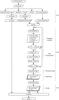 |
Fig. A.1 Flowchart illustrating the procedure for detecting vortex flows with the enhanced vorticity method and the vorticity strength method. |
All Tables
Performance results for the enhanced vorticity and the vorticity strength method based on tests with artificial vortex flows superimposed on a “realistic” simulated flow field.
All Figures
|
Fig. 1 Sample images illustrating the velocity distribution of a snapshot in our simulation (8 Mm × 8 Mm). a) LIC imaging scaled by the horizontal velocity amplitude, b) vorticity, c) LIC imaging scaled by the vorticity amplitude, and d) vorticity strength. Arrows indicate the velocity field. |
| In the text | |
|
Fig. 2 Comparison between LIC imaging, vorticity, and vorticity strength of a solid rotation (upper panels) and that of a shear flow (lower panels) indicated by white arrows. Upper panels: a) the horizontal velocity amplitude of a swirling feature is illustrated by the LIC imaging, b) the tangential discontinuity at the edge of a swirling feature is enhanced by the vorticity, and c) the constant angular rotation speed of a swirling feature is depicted by the vorticity strength. Lower panels: d) same as a) but for a shear flow, e) a gap between the rightward and leftward velocity at y = 0 is illustrated by the vorticity, and f) there are no features shown by the vorticity strength. |
| In the text | |
|
Fig. 3 Examples of the detection procedure for a vortex with a solid body rotation by using the enhanced vorticity method (left column) and the vorticity strength method (right column). The diameter of the rotating feature D0 is 200 km for a) and b), 400 km for c) and d), and 1000 km for e) and f), respectively. LIC imagings are shown in grey-scale in the background. Red and green crosses and circles indicate the location and the size of detected vortices, respectively. Thick crosses and circles mark the detections in the first iteration. |
| In the text | |
|
Fig. 4 Schematic illustration of how the detected features (red crosses in circles) are attributed to the same events in an image sequence. Orange, yellow, light-blue, and green circles indicate the identified events 1, 2, 16, and 17. The orange and yellow dashed lines illustrate the characteristic cone corresponding to a fixed characteristic speed (e.g. either the sound speed or the Aflvén speed). We choose to scan ten timesteps backwards to check the connectivity between the detected features and to confirm that they belong to the same event as illustrated for event 2. Involving several timesteps is important in case the event is not properly, or not all, detected in an intermediate timestep. In case of multiple detection candidates for the connectivity (e.g. multiple detections within a yellow dashed circle), we select the candidate being closest in terms of location and size. |
| In the text | |
|
Fig. 5 LIC imaging averaged over the sampled time period of 30 min in the simulation. The location of the test vortices are indicated by a black cross at (x, y) = (0, 0) and black circles with diameters of D0 = 200 km, 400 km, and 1000 km, respectively. The strong magnetic field region is indicated by a dashed contour line enclosing the region in which the time-averaged magnetic field strength is larger than the initial magnetic field strength of 50 G. |
| In the text | |
|
Fig. 6 Number of events detected with the vorticity strength method (grey curve) and with the enhanced vorticity method (black curve). The time-averaged numbers of events detected with the vorticity strength and the enhanced vorticity methods are 54.6 and 11.4, respectively. |
| In the text | |
|
Fig. 7 Histograms of a) the lifetime of the detected events and b) the maximum diameter of the detected events. In panel c), the lifetime is plotted versus vortex diameter. In panels a) and b), the results found with the enhanced vorticity method are plotted with grey bars, whereas results of the vorticity strength method are shown as black lines. For comparison, the chromospheric swirls found by Wedemeyer-Böhm et al. (2012) are plotted with red lines. In panel c, all events detected in the simulation are grouped according to their lifetime in bins of 1 min. For each group, the average value is plotted as a horizontal line ± one standard deviation, indicated by the shorter horizontal line above and below. The maximum values are plotted as diamonds. Again, the results of the enhanced vorticity method are plotted in grey, whereas the results of the vorticity strength method are shown in black. For comparison, the chromospheric swirls observed by Wedemeyer-Böhm et al. (2012) are plotted as red diamonds with numbers according to the table in the supplementary information of their study. In addition, the clearest swirl described by Wedemeyer-Böhm & Rouppe van der Voort (2009) is represented as a green diamond, whereas the range of swirl diameters found in that study is marked as a green shaded area. |
| In the text | |
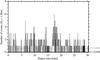 |
Fig. 8 Same as Fig. 6 but for the events whose diameter is larger than 1000 km. |
| In the text | |
|
Fig. A.1 Flowchart illustrating the procedure for detecting vortex flows with the enhanced vorticity method and the vorticity strength method. |
| In the text | |
Current usage metrics show cumulative count of Article Views (full-text article views including HTML views, PDF and ePub downloads, according to the available data) and Abstracts Views on Vision4Press platform.
Data correspond to usage on the plateform after 2015. The current usage metrics is available 48-96 hours after online publication and is updated daily on week days.
Initial download of the metrics may take a while.