| Issue |
A&A
Volume 601, May 2017
|
|
|---|---|---|
| Article Number | A31 | |
| Number of page(s) | 24 | |
| Section | Galactic structure, stellar clusters and populations | |
| DOI | https://doi.org/10.1051/0004-6361/201628967 | |
| Published online | 25 April 2017 | |
Determination of robust metallicities for metal-rich red giant branch stars
An application to the globular cluster NGC 6528⋆,⋆⋆
1 Lund ObservatoryDepartment of Astronomy and Theoretical Physics, Box 43, 221 00 Lund, Sweden
e-mail: This email address is being protected from spambots. You need JavaScript enabled to view it.
; This email address is being protected from spambots. You need JavaScript enabled to view it.
; This email address is being protected from spambots. You need JavaScript enabled to view it.
2 Key Lab of Optical Astronomy, National Astronomical Observatories, Chinese Academy of Sciences, A20 Datun Road, Chaoyang, 100012 Beijing, PR China
3 European Southern Observatory, 85748 Garching, Germany
Received: 19 May 2016
Accepted: 5 January 2017
Abstract
Context. The study of the Milky Way relies on our ability to interpret the light from stars correctly. With the advent of the astrometric ESA mission Gaia we will enter a new era where the study of the Milky Way can be undertaken on much larger scales than currently possible. In particular we will be able to obtain full 3D space motions of red giant stars at large distances. This calls for a reinvestigation of how reliably we can determine, for example, iron abundances in such stars and how well they reproduce those of dwarf stars.
Aims. Here we explore robust ways of determining the iron content of metal-rich giant stars. We aim to understand what biases and shortcomings the widely applied methods suffer from.
Methods. In this study we were mainly concerned with standard methods of analysing stellar spectra. These include the analysis of individual lines to determine stellar parameters, and analysis of the broad wings of certain lines (e.g. Hα and calcium lines) to determine effective temperature and surface gravity for the stars.
Results. For NGC 6528 we find that [Fe/H] = + 0.04 dex with a scatter of σ = 0.07 dex, which gives an error in the derived mean abundance of 0.02 dex.
Conclusions. Our work has two important conclusions for analysis of metal-rich red giant branch stars. Firstly, for spectra with S/N of below about 35 per reduced pixel, [Fe/H] becomes too high. Secondly, determination of Teff using the wings of the Hα line results in [Fe/H] values about 0.1 dex higher than if excitational equilibrium is used. The last conclusion is perhaps unsurprising, as we expect the NLTE effect to become more prominent in cooler stars and we can not use the wings of the Hα line to determine Teff for the cool stars in our sample. We therefore recommend that in studies of metal-rich red giant stars care should be taken to obtain sufficient calibration data to enable use of the cooler stars.
Key words: Galaxy: bulge / globular clusters: individual: NGC 6528 / stars: atmospheres / stars: fundamental parameters
Based on observations made with the ESO/VLT, at Paranal Observatory, under programme 067.B-0382(A) and on data obtained from the ESO Science Archive Facility under programme 065.L-0340(A), 067.D-0489(A), and 077.B-0327(A) and from the Keck Observatory Archive under programme C53H and C19H.
The reduced spectra is only available at the CDS via anonymous ftp to cdsarc.u-strasbg.fr (130.79.128.5) or via http://cdsarc.u-strasbg.fr/viz-bin/qcat?J/A+A/601/A31
© ESO, 2017
1. Introduction
The analysis of red giant branch star spectra is problematic. As we progress along the red giant branch upwards to cooler and lower gravity stars, a number of phenomena begin to appear more and more strongly in the spectra. In particular, the atomic lines get stronger, causing more blends and the cooler atmospheres allow for the formation of molecules such as TiO, CN, and MgH resulting in strong molecular features. This makes it progressively more and more difficult to find (or define) the continuum in the spectrum. As many methods rely on the identification of the continuum, this causes a problem.
Our main aim with the present investigation is to study how we can, in a robust way, determine the iron abundance for metal-rich giants, such as those seen in the Galactic bulge and old, metal-rich globular clusters. We are interested in providing a better understanding of the influence on the derived iron abundance from the signal to noise ratio (S/N) in the analysed spectra and any influence on the method used to determine the other stellar parameters, for example, Teff and log g, on the final iron abundance.
The study of the Milky Way has in the last couple of decades become a major area of astrophysics. This is due to two influential astrometric missions: the completed Hipparcos mission (Perryman et al. 1997) and the current Gaia mission (Perryman et al. 2001; Brown 2013, where the first paper describes the concept behind the Gaia proposal to the European Space Agency and the second paper gives an overview of, Gaia just before launch). The Hipparcos catalogue enabled a new type of study, allowing determination of accurate velocities and ages for samples consisting of many hundreds of stars near the sun (e.g. Bensby et al. 2004, 2014; Soubiran & Girard 2005; Fuhrmann 2011; Adibekyan et al. 2012, 2013). These studies were performed on F and G dwarf stars. However, Gaia will provide data of the same quality as Hipparcos for a significantly larger volume of the Milky Way, reaching all the way into the Galactic bulge. However, the stars available for spectroscopic work will (as of today) be the red giant branch stars, as these are intrinsically bright enough to be observable with current instrumentation at a distance of 8 kpc. The only option to obtain spectra for dwarf stars in the Galactic bulge is currently to take advantage of microlensing events (e.g. Bensby et al. 2013). This is, however, not an option if we want to study large samples. Thus it remains important to study how we best can robustly determine stellar parameters and elemental abundances of evolved red giant stars. This paper deals with this topic.
The spectroscopic and photometric data Gaia benchmark stars and stars in the metal-rich globular cluster NGC 6528 are presented in Sect. 2. Our basic tools and linelist are described in Sect. 3. To determine stellar parameters for red giants we explore different methods and test them on the benchmark stars in Sect. 4. In Sect. 5 we apply our analysis to stars in NGC 6528 and discuss problems in the analysis. In Sect. 6, we determine [Fe/H] for NGC 6528. Section 7 provides our conclusions and discusses future developments.
2. Description of data
2.1. Spectra
2.1.1. Benchmark stars
To determine the best analysis techniques for metal-rich cool giant stars we used star spectra that have well-determined stellar parameters, those of the so called Gaia benchmark stars (Heiter et al. 2015a). There is a wealth of high quality data available, in particular they have interferrometric observations enabling a direct determination of their radii and effective temperatures (Teff). As we are interested in metal-rich stars, we selected ten red giants which have iron abundances greater than –0.55 dex (Jofré et al. 2014). The ten stars, which have Teff similar to the stars of NGC 6528, are Arcturus, μLeo, HD 107328, βGem, ϵVir, ξHya, αCet, γSge, αTau, and βAra. Their stellar parameter reference values are listed in Table 2.
The fifteen called “initial resolution” that have high S/N (>250) were taken from a high resolution spectral library for benchmark stars (see more details in Blanco-Cuaresma et al. 2014). The library consists of observations taken from UVES (Dekker et al. 2000), HARPS (Mayor et al. 2003) and NARVAL (Aurière 2003) spectrographs. It should be noted that five stars (μLeo, βGem, ξHya, αCet, and γSge), have one spectrum each, while the rest of stars have two spectra observed in different instruments. For example, the star Arcturus was observed with the NARVAL and UVES spectrographs, while βAra was observed with the HARPS and UVES spectrographs.
2.1.2. Stars in NGC 6528
Basic data for NGC 6528.
Stellar parameters for the Gaia benchmark stars.
The basis for our study of stars in NGC 6528 is our own 2001 observations of seven stars. In order to have a statistically significant sample of spectra of red giant stars in NGC 6528 we further searched the ESO and the KECK archives. In the archive we found spectra of 34 stars that are potential members of NGC 6528. Of these 12 have been observed by UVES on VLT in stand-alone mode, 20 with UVES as part of FLAMES observations, and two stars had been observed with HIRES on KECK. Table A.1 lists basic information about the stars and observations. There is no overlap between the observations from the different programmes. Below we describe the different data-sets in some detail.
Stars observed with UVES:
our starting data-set consists of observations of seven stars carried out in 2001 at the VLT 8-m telescope using the UVES spectrograph (Dekker et al. 2000) under our programme 067.B-0382(A) (PI: S. Feltzing). The stars were selected as members of NGC 6528 based on a proper motion study using high-resolution images and VI photometry from HST (see Feltzing & Johnson 2002). In the ESO archive we found an additional five stars observed with UVES from programme 065.L-0340(A) and 067.D-0489(A) (PI: D. Minniti). These were all observed in 2000 and 2001, respectively.
The resolution of the observations is 45 000 or 55 000 in the red arm (480–680 nm) depending on the slit width used (0.8′′ or 1.0′′). The observations were all done using the standard setup 580 with CD #3. The exposures have been split in order to allow for the removal of cosmic ray hits. The data were reduced using the UVES pipeline (Ballester et al. 2000), including bias, inter-order background subtraction, flat field correction, extraction, and wavelength calibration. All the echelle orders were then merged into a 1D spectrum for each exposure.
In the archive we found 20 stars which are potential members of NGC 6528 from programme 077.B-0327(A) (PI: M. Zoccali) which was observed in 2006. The multi-object optical spectrograph FLAMES (Pasquini et al. 2002) has two parts, one being FLAMES-UVES which has eight robotic fibers which feed the UVES spectrograph at VLT. The spectra have R ~ 47 000 and the observations were done with the setup centred at 580 nm (wavelength coverage: 480–680 nm). We reduced the raw frames using the FLAMES-UVES pipeline in a standard way. After all the recipes, which include creating a master bias and the master slit flat-field frame, determining the fiber order table, the wavelength solution, and extracting the science frame, of the pipeline have been executed we subtract the sky background spectrum from the stellar spectra. For FLAMES-UVES the sky background is usually observed by one fiber placed in an empty part of the sky. With the sky background removed, we shifted the sky-subtracted spectra to a heliocentric reference frame making use of the packages RVSAO and DOPCOR within IRAF1.
To improve the S/N, we co-added all the UVES spectra of the same star into a single spectrum. The average S/N of the final co-added spectrum for each star was estimated by making use of the SPLOT task within IRAF at three short wavelength regions (574.4−574.7 nm, 604.7−606.3 nm, and 606.8−607.6 nm). For most spectra, S/N is greater than 30 per pixel (see Table A.1).
Stars observed with HIRES:
we collected spectra of two red horizontal branch stars (3014 and 3025) from the Keck Observatory archive. The observations were taken with HIRES (Vogt et al. 1994) at Keck I under the programme C53H and C19H (PI: J. Cohen) in 1999 and 2000, respectively.
Since the HIRES detector is not large enough to yield full spectral coverage, there is a gap (1.0−6.0 nm) between any two echelle orders. The raw spectra were reduced using the MAKEE2 package. This package determines the position of each echelle order, defines the object and background extraction boundaries, optimally extracts a spectrum for each order, and compute wavelength calibrations non-interactively. We co-added the spectra of each star into one spectrum. The measured mean S/N of the co-added spectra was estimated in the same way as for the UVES spectra (Table A.1).
2.2. Additional data for NGC 6528
2.2.1. Photometry
In order to estimate good starting values for Teff for our stars we made use of colour-temperature-metallicity relations. To this end we collected near-infrared photometric data from 2MASS (Cutri et al. 2003) and VVV (VISTA Variables in Via Lactea) (Minniti et al. 2010).
The survey area of VVV is fully imaged in five photometric bands: Z,Y,J,H,Ks and 2MASS has imaging in J,H,Ks. The VVV survey goes about four magnitutes deeper than 2MASS. However, the larger telescope aperture of VISTA results in saturation for the brightest stars. The saturation magnitude in the VVV photometry occurs at Ks< 12. We therefore adopt 2MASS photometry for stars brighter than 12 mag in Ks and we require that the photometric quality flag is AAA (the highest quality). For all other stars we use VISTA photometry.
There is a very small offset between the zero-points of the VVV and 2MASS catalogues. To ensure that all photometry is on the same system we have chosen to transfer the VVV photometry onto the 2MASS photometric system as this is the system most commonly used in the available temperature calibrations. The following zero-point offsets have been applied: (J2mass−Jvvv) = 0.029; (H2mass−Hvvv) = −0.039; (Ks,2mass−Ks,vvv) = −0.028 (Gonzalez et al. 2011).
2.2.2. Reddening
Reddening is important for the initial estimate of Teff, but it can also be of interest when discussing the properties of the cluster. Here we make use of the recent reddening maps by Gonzalez et al. (2011, 2012) to estimate the reddening towards our stars.
As the maximum sky resolution of the reddening map is 2′, we assumed that the stars are subject to the same reddening within a 4′ × 4′ box. The observed targets are spread in a relatively large area, the total coverage of the dereddened region is 28′ × 28′ consisting of 49 boxes of 4′ × 4′. The mean extinction, AKs, and colour excess, E(J−Ks), are calculated using BEAM3 which uses the extinction law from Cardelli et al. (1989). The adopted coefficients for J,H, and Ks (in the 2MASS passbands) are: AJ = 1.692E(J−Ks), AH = 1.054E(J−Ks), AKs = 0.689E(J−Ks). Where AKs = 0.689E(B−V). The dereddened magnitudes of J,H, and Ks are listed in Table A.1.
2.2.3. Radial velocities
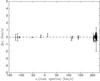 |
Fig. 1 Comparison of radial velocities for the stars derived from the combined spectrum and from the individual spectra separately and then averaged (see Sect. 2.2.3). The x-axis shows the value derived from the combined spectra whilst the y-axis shows the difference between vr determined in the two ways. The error-bars for the difference is the coadded errors estimated from IRAF (for the combined spectra) and the σ around the mean for the independent measures. Errors on the x-axis are too small to be seen. |
Radial velocities (vr) with respect to the Sun were derived using the RVSAO package within IRAF. The XCSAO task cross-correlates a template spectrum with the observed spectrum and reports the velocity difference between the two. Here we used a template spectrum from the radial velocity standard star ϵPeg. The resolution of the spectrum is similar to that for the spectra of our sample spectra.
Each of our stars have more than one observation (Table A.1). The spectra are often taken at different nights and sometimes even months apart. This allows us to derive vr in two ways, enabling a test of the quality of our results. First we extracted all spectra and corrected them for Earth’s motion in order to co-add them. Radial velocities were then determined using these combined spectra. In the other approach, we derived the radial velocity for each observation individually. These individual measurements were then averaged and the scatter around the mean was calculated. Typically, the scatter around the mean radial velocities is less than 0.50 km s-1. We find that the two approaches give very similar results (compare Fig. 1).
For unknown reasons, we are unable to recover the radial velocities determined by Carretta et al. (2001) for stars 3014 and 3025. Our results are about 50 km s-1 larger than the values given by them. As far as we understand, we are using the same spectra and same reduction software. In Table A.1 we list the value from Carretta et al. (2001). Apart from this difference, our derived velocities agree well with those in the literature (see Sect. 2.3).
2.3. Membership
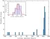 |
Fig. 2 Distribution of measured heliocentric radial velocities for our programme stars. The inset in the top-left corner shows a zoom-in high-lighting the velocity distribution of the cluster members fitted by a Gaussian. The red cross indicates the mean (212.1 km s-1) and standard deviation (4.2 km s-1) of the radial velocity for the cluster members. |
Membership of globular clusters for individual stars is commonly determined using radial velocities (e.g. Simmerer et al. 2013) or proper motions relative to the background and foreground stars (e.g. Zoccali et al. 2001). NGC 6528 has a radial velocity of ~210 km s-1 (Carretta et al. 2001; Zoccali et al. 2004) and a proper motion relative to the background bulge population of ⟨ l ⟩ = 0.006 and ⟨ b ⟩ = 0.044 arcsec per century (Feltzing & Johnson 2002). This means that radial velocity is the best way to determine membership for this cluster. Using measurements from the luminous stars in globular clusters, as well as their integrated spectra, Pryor & Meylan (1993) determined the velocity dispersions for many globular clusters. They found that typical velocity dispersions in globular clusters is less than 10 km s-1.
Figure 2 shows the distribution of radial velocities for all our stars. There is a clustering of stars just above 200 km s-1. To find the mean velocity and velocity dispersion of NGC 6528, we began by considering stars with a radial velocity in the range 155−240 km s-1. For these we calculated the mean and standard deviation (σ) of the radial velocity. We then proceeded to exclude stars more than 3σ from the mean value and the mean and σ were re-calculated. This procedure was iterated until no more stars could be excluded with a 3σ-clipping. This left 26 stars for which we found a mean velocity of 212.1 km s-1 and σ = 4.2 km s-1. Our velocity dispersion is in good agreement with the value of 4.0 km s-1 measured by Carretta et al. (2001).
3. Linelist and analysis tool
3.1. Line list
To assemble the line list we made use of several sources. For iron we selected 106 clean lines between 470 nm and 690 nm from Tsantaki et al. (2013), Den Hartog et al. (2014), and the linelist compiled for the Gaia-ESO survey (Heiter et al., in prep., and references therein; see also, Heiter et al. 2015b). In particular, we selected 90 Fe i and 16 Fe ii lines. All our lines were examined in the spectra of the Sun and ξHya. ξHya is a relatively cool and metal-rich star with stellar parameters similar to those in our sample of stars in NGC 6528 and stars in the Galactic bulge (compare values in Table 3). Firstly, these two spectra were used to check that the lines are clean and possible to analyse in metal-rich giant stars. Secondly, the equivalent width (EW) of lines in the two stars were measured. Because the strong lines are sensitive to the selection of the microturbulent velocity (Fulbright et al. 2006) and might suffer from the effects of improper modelling of the outer layers in stellar atmosphere models (McWilliam et al. 1995), all lines with EWs higher than 130 mÅ were removed from our line list.
As cool and metal-rich stars have more molecular lines than warmer stars, we make an extra check to make sure that our lines are not blended by molecules. For this check, we used the spectrum synthetic programme (see described in Sect. 3.2) and the complete VALD (Kupka et al. 2000, 1999, see also references in the data-base) line list containing all metal and molecular lines to compute a synthetic spectrum. To generate a spectrum of a cool and metal-rich giant, the typical stellar parameters (Teff = 4500 K, log g = 2.0, [Fe/H] = +0.1 dex) were interpolated in the MARCS model atmospheres (Gustafsson et al. 2008). We examined all the lines by eye and found that most of them are free of TiO, CN, C2, and MgH within 0.2 mÅ of the centre of the Fe line. Sixteen Fe lines might suffer a weak contamination from the CN lines. This suggests that our final measured stellar parameters and abundance should not have a large systematic errors caused by the blending of molecular lines.
The oscillator strength (log gf) for the Hα line is adopted from the VALD database. The atomic data for the Ca i lines are taken from Smith & Raggett (1981), apart from the log gf values for Ca i 612.2 and 616.2 nm, which are from Aldenius et al. (2009). The full list of lines, including references to atomic data, can be found in Table B.1.
3.2. Spectral anlaysis – SME
We use Spectroscopy Made Easy (SME, Valenti & Piskunov 1996; Valenti & Fischer 2005) to determine the stellar parameters by comparing synthetic spectra with observed spectra. SME uses the Levenberg-Marquardt (LM) algorithm to optimise stellar parameters by fitting observed spectra with synthetic spectra. The LM algorithm combines gradient search and linearization methods to determine parameter values that yield a chi-square (χ2) value close to the minimum. Stellar parameters and atomic line data are required to generate a synthetic spectrum. In addition to specified narrow wavelength segments of the observed spectrum, SME requires line masks in order to compare with synthetic spectrum and determine velocity shifts, and continuum masks that are used to normalise the spectral segments. The homogeneous segments and masks are created to fit all of our solar sibling candidates.
SME requires input values for Teff, log g, [Fe/H], microturbulence (vmic), macroturbulence (vmac), and rotational velocity (vsini). Given initial stellar parameters, the model atmospheres are interpolated in the precomputed MARCS model atmosphere grid, which has standard composition of elemental abundances. We then configured SME to fit each stellar spectrum by adjusting the free parameters (see Sect. 4). The convergence is (likely) speedier if we start with realistic initial values. However, it should be noted that SME is capable of converging to the correct values also if we start from initial values that are far off from the correct ones (Daniel Adén, priv. comm., tests for the Gaia-ESO Survey).
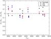 |
Fig. 3 Test of the ability of our linelist to reproduce the reference [Fe/H] for the Gaia benchmark stars. The y-axis shows the difference between the reference value and the value we derive (using the reference Teff and log g, but our own linelist and SME). We derived [Fe/H] in three ways: using both Fe i and Fe ii lines (blue filled squares), using only Fe i lines (red filled circles), and using only Fe ii lines (black filled triangles). The stars can be identified using the Teff values which are given on the x-axis. For some of the stars we have more than one spectrum. Results for both are shown in the plot. |
Before starting our investigation, we first checked how well our set-up and linelist reproduces the reference values for [Fe/H] for the benchmark stars.
To this end, we analysed the spectra fixing Teff and log g to the recommended values (Table 2). We did three sets of analysis: one where both Fe i and Fe ii lines were fitted, one where only Fe i lines were fitted, and one where only Fe ii lines were fitted. In each case all lines were all fitted simultaneously.
The results are shown in Fig. 3. We find that when we fit Fe i and Fe ii lines simultaneously the difference between our values and the recommended values is 0.01 dex with a σ of 0.10 dex. In Fig. 3 we can see that it is the coolest stars that drives the size of the scatter, whilst the warmer stars have a smaller difference. When we fit only the Fe i lines the difference is 0.01 dex with a σ of 0.07 dex, and when we analyse the Fe ii lines only we find a difference of 0.03 dex with a σ of 0.07 dex. There are no discernible trends with Teff, although there is a weak indication that Fe ii lines do a better job in reproducing the reference values for the coolest stars (αCet, γSge, and αTau) while in the warmest stars (βGem, ϵVir, and ξHya) Fe i lines appear to do a much better better job than the Fe ii lines. However, the trend is weak and more data would be needed to draw a firm conclusion regarding if certain species are better at a certain temperature range for these types of stars. This comparison shows that our line data and method of analysing the iron lines (assuming all other parameters to be known) is fully compatible with those in Jofré et al. (2014) who has established the reference values for the Gaia benchmark stars.
4. Looking for a robust method to determine [Fe/H] for metal-rich red giant stars from optical spectra
4.1. Methods to derive effective temperature
Effective temperatures can be derived from stellar spectra using several methods. Fe i is the most common ion in terms of lines in the optical spectrum. As lines arising from the Fe i ion have a wide range of line strengths as well as excitation potentials it is in principle straightforward to determine Teff for the star by requiring Fe i lines with differing excitation potentials to produce the same iron abundances (e.g. Edvardsson et al. 1993). This analysis rests on the assumption of local thermal equilibrium (LTE). However, several studies suggest that this assumption does not necessarily hold (e.g. Fuhrmann 1998; Thévenin & Idiart 1999; Mashonkina et al. 2011; Ruchti et al. 2013). Recently, NLTE calculations, for example, from Bergemann et al. (2012), have been included into some studies (e.g. Ruchti et al. 2013). However, at solar metallicities the difference between LTE and NLTE results for Fe i tend to be very small for metal-rich stars (Ruchti et al. 2013) and we can thus neglect them here. Determination of the iron abundance is a by-product when Teff is derived in this way and errors in the Teff and iron abundance must correlate.
Another method to derive Teff is to use the strong hydrogen lines present in stellar spectra as these lines change rapidly in strength as a function of Teff. These lines also have no gravity dependence in cool stars. Most commonly, Teff is derived from the synthesis of the extended wings of the Hα and Hβ lines (e.g. Barklem et al. 2002; Ruchti et al. 2013). This makes them very useful for determining the temperature for stars with Teff< 8000 K (Gray 2005). With this method iron must be determined independently and hence the errors are not correlated.
Another approach is to use line-depth ratios to derive Teff (Gray 1994). One advantage of using line-depth ratios is that these do not depend on the metallicity of the star. In the visible spectral range, unblended Si, Ti, V, Cr, Fe and Ni line-depth rations can be used to estimate Teff. There are not many applications of this method in the literature, but Kovtyukh & Gorlova (2000) illustrated that the line-depth ratios are powerful indicators of Teff at least for supergiants. We will not further explore this method here.
Finally, we can use calibration of stellar photometry to derive Teff from a colour index, such as (B−V)0 (see, e.g. González Hernández & Bonifacio 2009). This method has its limitations. For example, for stars in the Galactic bulge or in the plane of the Galaxy the photometric approach is hampered by the poorly determined reddening of individual stellar colours. Although this method is not very dependable for bulge stars, thanks to the large reddening along the line-of-sight, it nevertheless provides useful starting values for our analysis.
4.2. Methods to derive surface gravity
It is common to measure log g by imposing ionization equilibrium which means that we require Fe i and Fe ii lines to produce the same abundance4. Fe ii lines can be weak and they are not as numerous as the Fe i lines. This method thus requires high-quality spectra with large wavelength coverages. As discussed above (Sect. 4.1), Fe i lines can be susceptible to departures from LTE. This is not true for Fe ii lines. Which means that ionizational balance can be influenced by departures from LTE. Determination of the iron abundance is a by-product of this method and errors in log g and [Fe/H] must correlate.
Several lines show strongly pressure-broadened wings in the spectra of cooler stars. This means that the surface gravity of late-type stars can be determined from analysis of these lines. Lines that have pressure broadened wings include the Mg i b lines at 516.7, 517.2, 518.3 nm, the Na i D lines at 588.9 and 589.5 nm, and the Ca i lines at 612.2, 616.2, and 643.9 nm (see, e.g. Edvardsson 1988; Bonnell & Bell 1993; Fuhrmann et al. 1997; Jönsson et al. 2017). The analysis of the wings of these strong lines require that the elemental abundance of the element the line is arising from is also determined, from other lines than the one used to derive log g. This means that errors in log g and the abundance of that element correlate. Finally, when we have independent measurements of Teff and metallicity, log g can be derived through isochrone fitting (see, e.g. Sozzetti et al. 2007). We will not further explore this method here.
4.3. Determining stellar parameters
In Sects. 4.1 and 4.2 we discussed various ways to determine Teff and log g. Although this is not an exhaustive summary, combining the various ways to derive Teff and log g still leads to quite a few possible combinations. Here we will explore the following combinations:
-
Method 1:
in this method we only use Fe i and Fe ii lines to constrain all stellar parameters (i.e. excitation and ionizational equilibria are imposed).
-
Method 2:
in this method we use the Hα line to constrain Teff, the strong Ca i lines to constrain log g, and Fe i lines to derive the iron abundance.
-
Method 3:
in this method we use the Hα line to constrain Teff, the strong Ca i lines to constrain log g, and Fe ii lines to derive the iron abundance.
While in Method 1 all parameters are correlated, Methods 2 and 3 aim at breaking these degeneracies by using separate measures for each of the three main parameters. We did not attempt to use the Mg i b and Na i D lines as these are too blended by the atomic and molecular lines to determine log g from them in metal-rich giant stars as we are interested in here. For cool giants with Teff< 4400 K, we further found that the wings of the Hα line almost vanished (see also Appendix C). This lead us to modify Method 2 to be able to include also such stars in our study (see Sect. 4.3.2). In addition to Teff, log g, and [Fe/H] a spectroscopic analysis normally calls for the determination of a few other parameters; microturbulance (vmic), marcotublence (vmac), and rotational velocity (vsini).
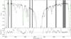 |
Fig. 4 Comparison of synthetic spectra with the wings of Hα line in ϵVir. The middle synthetic spectrum (in red) shows the best fit. The other two synthetic spectra (blue and green) indicate the shape of the wings when Teff is changed according to our estimated uncertainty (here 50 K). The grey areas mark the regions used to evaluate the goodness of the fit. Note that these are relatively narrow since the spectrum has very little clean “line continuum” thanks to the cool temperature of the star, which results in many lines being present in the spectrum. |
Microturbulance and macroturbulence can either be derived from the spectrum itself or obtained from a calibration, such as those in Jofré et al. (2014). Rotational velocities of red giants and horizontal branch stars are typically small (vsini < 5 km s-1), therefore a good assumption is to set vsini to 1 km s-1. Which is what we do for the rest of this paper. We note that there is often a degeneracy between vsini and vmac which is hard to break in the analysis. For the type of study presented here – where the aim is to get the best measure of [Fe/H] – the exact values of these two parameters is of less relevance to the final outcome of the investigation and we can allow them to be degenerate. This implies that in this study we can regard them (together) as nuisance necessary to the fit but not necessarily giving physical insight in to the star. To test the three methods we adopted ten benchmark stars (see Heiter et al. 2015a; Jofré et al. 2014, and Sect. 2.1.1).
4.3.1. Method 1: Fe i and Fe ii lines
In this method we fit all free parameters simultaneously by comparing the observed spectrum with a synthetic one for short regions around the Fe i and Fe ii lines. It should be mentioned that the method is more commonly performed with equivalent widths in the literatures (e.g. Bensby et al. 2003). This method is speedier if we start with realistic initial values for stellar parameters (see also Sect. 3.2). For the benchmark stars, their recommended values are used as the initial input, however, experience shows that the exact values are unimportant to achive convergence. An initial value for vmic was obtained using the relation given in Jofré et al. (2014). The initial vmac value was set to 5.0 km s-1 for all stars.
All parameters are simultaneously fitted inside SME. As SME strives to fit all lines equally well this is in effect the same as requiring ionizational and excitational equilibrium – hence, all parameters are determined simultaneously. The method differs slightly from its most common implementation in the literature where an iterative scheme is employed and one parameters is varied in each step (see, e.g. Drake 1991; Drake & Smith 1991, and discussions therein). Instead, the usage of SME in fully free mode is more akin to the method used in Feltzing et al. (2009) where the parameter space is searched (by hand) for a best fit to all criteria simultaneously.
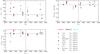 |
Fig. 5 Comparison of the stellar parameters derived using the three methods discussed in Sects. 4.3.1 till 4.3.3 with the reference values (Table 2). On each y-axis is indicated the difference between the values we have obtained and the reference value (indicated by a subscript “r”). Method 1 is indicated by red symbols, Method 2 by black, and Method 3 is indicated by cyan symbols. Different symbols represent the different stars (as indicated in the figure, note that each symbol represent two stars. They should be easy to identify thanks to their different Teff). Note that some stars have more than one spectrum analysed (see Sect. 2.1.1). The stars can be identified by their recommended Teff which is plotted on the x-axis. The dashed line indicates the separation of “cool” (left) and “warm” (right) giants (see Sect. 4.3.2). |
4.3.2. Method 2: Hα, Ca, and Fe i lines
To break the degeneracy between the different parameters we use different spectral indicators for each of the main stellar parameters. This method requires a set of initial parameters to get started. These could be obtained in different ways (e.g. from photometry). For this test we take the parameters obtained in Method 1 as initial input.
Method 2: for warm giants (Teff> 4400 K), the following steps are used:
-
1.
define a set of parameters as initial input;
-
2.
fit the wings of Hα to derive Teff, while the other parameters are kept fixed;
-
3.
fit the wings of the three strong Ca i lines (λ 612.2, 616.2, and 643.9 nm) to determine log g. To break the degeneracy of log g and Ca abundance, several weak Ca i lines are also fitted at the same time;
-
4.
derive [Fe/H] from the Fe i lines by setting both vmic and vmac free, while the other parameters are kept fixed at the values derived in the steps above;
-
5.
repeat steps 2 to 4 with updated parameters until all five parameters reach convergence, including Teff, log g, [Fe/H], vmic and vmac.
For step 2, a number of synthetic spectra are generated and their fit is evaluated using the spectral regions indicated in Fig. 4. Further examples can be found in Appendix C.
In Step 3 the three strong Ca i lines are simultaneously fitted. It would be possible to fit them each individually instead. A discussion of the merits of the different approaches can be found in Appendix D.
Step 5 requires us to decide when a given parameter has converged. For the current work the following convergence criteria were applied: between two iterations the differences should be ΔTeff< 50 K for most stars, but for stars with very high S/Ns we required <20 K, Δlog g < 0.05 dex, and Δ[Fe/H] < 0.05 dex.
As mentioned, it is not feasible to measure Teff from the Hα line for the cooler giants (Teff< 4400 K). Therefore, the only option is to derive Teff using Fe i lines (excitational equilibrium) rather than the wings of the Hα line for these stars. However, this re-introduces a degeneracy between Teff and [Fe/H]. We are still able to use the three strong Ca i lines to determine log g.
Modified Method 2: for cool giants (Teff < 4400 K, the following steps are used:
-
1.
define a set of parameters as initial input;
-
2.
fit the wings of the three strong Ca i lines (λ 612.22, 616.22, and 643.91 nm) to determine log g. To break the degeneracy of log g and Ca abundance, several weak Ca i lines are also fitted at the same time;
-
3.
set both vmic and vmac as free parameters while keeping log g fixed, we only fit Fe i lines to determine Teff and [Fe/H] at the same time;
-
4.
repeat steps 2 to 3 with updated parameters until all five parameters converge.
4.3.3. Method 3: Hα, Ca, and Fe ii lines
Since the only difference between Method 3 and Method 2 is that we use Fe ii rather than Fe i lines, the atmospheric parameters are measured making use of the same iterative process described in Sect. 4.3.2 by changing from Fe i line to Fe ii lines.
For Modified Method 2 we did make use of excitation equilibrium using the Fe i lines. However, the number of Fe ii lines available is much fewer than Fe i lines and they do not cover a large enough range in excitation potential for us to try to determine Teff from excitation equilibrium. Method 3 is thus only implemented for warm giants (Teff> 4400 K).
4.4. Discussion and error estimates
We now proceed to compare our results for the ten benchmark stars derived using the three methods. A comparison is shown in Fig. 5 and the stellar parameters obtained using Method 2 and Modified Method 2 are listed Table 2. In particulare we find5:
-
Method 1: ΔTeff = 56 K (σ = 79), Δlog g = −0.04 (σ = 0.20), andΔ [Fe/H] = 0.03 dex (σ = 0.11);
-
Method 2: ΔTeff = 35 K (σ = 54), Δlog g = 0.02 (σ = 0.07), and Δ [Fe/H] = −0.03 dex (σ = 0.08);
-
Method 3: ΔTeff = 19 K (σ = 53), Δlog g = −0.03 (σ = 0.08), and Δ [Fe/H] = 0.04 dex (σ = 0.04) (warm giants only).
Of the three methods, Method 1 clearly performs the least well. It is noticeable that the scatter in all three stellar parameters are quite a bit higher for this method than for the other two. The offsets are also somewhat larger. From Fig. 5 we see that there is no particular trend in ΔTeff, Δlog g, and Δ[Fe/H] as a function of Teff. This is reassuring as it indicates that our methods do not have hidden trends in them and that the estimated scatters can be trusted.
Method 3 suffers from the shortcoming that it can not be applied to cooler giants (Teff< 4400 K). This is a severe limitation for the study of globular clusters and field giants in the Galactic bulge. To study the metallicity distributions, we would therefore recommend Method 2 as providing a sound basis for an analysis of a large sample of stars. It is reassuring that this method not only gives good metallicity estimates but also reliable stellar parameters in general.
The uncertainty in Teff can be estimated by inspecting the comparison of synthetic spectra with the observed spectrum. This is relatively straightforward for the high S/N and high resolution spectra we have for the Gaia benchmark stars. We found that the typical uncertainty in Teff is about 50 K for most of the warm giants. One example, ϵVir, is shown in Fig. 4. For log g, we found that for most stars the typical uncertainty is around 0.10 dex (see more details in Appendix D).
For [Fe/H] we calculated the error in the mean by using the iron abundance from each iron line individually (remember that the parameters are decoupled in this method). Calculating the formal error in the mean we find errors typically around 0.02 dex, whilst σ is just below 0.1 dex (see Table 2).
For the benchmark stars, the typical uncertainties in the recommended Teff and log g are about 60 K and 0.10 dex (Heiter et al. 2015a), respectively. The scatter in Teff and log g around the recommended values for the benchmark stars found in this study is comparable with the typical uncertainties of the recommended stellar parameters. There is a very small offset between the recommended [Fe/H] and our results when using Method 2. The typical uncertainty in the recommended [Fe/H] is comparable to what we find (<0.02 dex, Jofré et al. 2014).
4.5. How much do the results depend on the S/N in the spectra?
Our tests of different methods have relied on the analysis of high S/N spectra of the metal-rich, cool giants in Gaia benchmark sample. Clearly, a study of for example the Galactic bulge will have spectra of much lower S/N. How will this influence the results? We analysed this in two steps. Firstly we will degrade the spectra for the Gaia benchmark stars to mimic that of high quality data for stars in the Galactic bulge and secondly we will make use of the extensive data set of stars in NGC 6528 that we have collected.
To test the dependence of our final results on S/N and resolution we have degraded the spectra for the ten benchmark stars and re-analysed them. We chose 45 000 and 20 000 for the resolution and at three different S/N (25, 35, 45). 20 000 is a resolution that is common for FLAMES-GIRAFFE (used in the Gaia-ESO Survey) and the future massively multiplex spectrographs (e.g. WEAVE and 4MOST, Dalton et al. 2014; de Jong et al. 2014, respectively).
Comparing with the results derived from the original spectra we found that [Fe/H] is weakly overestimated when the spectra are noisier, but [Fe/H] does not depend on the resolution of the spectrum. We note that we did not investigate whether the abundances of other elements were unaffected. The iron lines we use were carefully selected to be the cleanest and most easy to analyse, but for other elements this may not be true.
5. Applying our analysis to stars in NGC 6528
5.1. Stellar parameters for NGC 6528 stars
Initial Teff for the stars were calculated using the colour-Teff-[Fe/H] relation from González Hernández & Bonifacio (2009). As we could not obtain photometric data in the optical for all our stars, the dereddened J−Ks colour is used to calculate the initial estimate of Teff. Following previous studies of the metallicity of NGC 6528 (e.g. Zoccali et al. 2004), we set [Fe/H] = −0.10 dex as the initial value for the analysis for all stars. Since most of our stars are either horizontal branch or red clump stars, we simply set the initial log g to 2.5 dex for warm giants (Teff ≥ 4400 K) and 2.0 dex for the cooler. For the analysis we used Method 2 and Modified Method 2, as desribed in Sect. 4.3.2.
Inspecting the spectrum of star 1–24, we found that most of the lines are asymmetric. Zoccali et al. (2004) found that this star likely is a binary. Our inspection of the spectrum supports this conclusion. The star was removed from our sample.
For stars 61, 66, 68, and 84 we were unable to analyse the spectra as they all have low S/N and in addition the spectra appear to have several unexpected features. These stars were excluded from the analysis.
This leaves us with 29 successfully analysed stars. The results are listed in Table 3. Eight of these stars are not radial velocity members of NGC 6528 (see Sect. 2.3).
Stellar parameters for the sample stars derived using Method 2.
5.2. Analysis of a suite of low S/N spectra for stars in NGC 6528
For several of the stars in NGC 6528 we have multiple exposures. This allowed us to analyse spectra of different S/N for the same star. Using Method 2 and Modified Method 2 we analysed the actual observed spectra of five stars (star-05, -07, -62, -65 and -67, IDs as in Table A.1).
Two of the cluster stars (-62 and -71) have a large number of spectra allowing us to study the results in a more statistical way. As reference value we used the final parameters determined for each star as listed in Table 3.
We find that the scatter for a given star as well as for the whole sample, increases as we go to spectra with lower and lower S/N. This is not a new finding, but it is here quantified in detail for what we believe is the first time for evolved, metal-rich giant stars. Although the scatter increases as we go to lower S/N the mean value of the measurements more or less reproduces the reference value. At the lowest S/N we find a positive offset (Fig. 6). Further details are available in Appendix E.
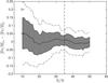 |
Fig. 6 Difference between [Fe/H] derived from spectra of varying S/N (per pixel) for stars in NGC 6528. [Fe/H]x indicates our value measured for each spectrum, while [Fe/H]r indicate the value obtained in Sect. 5.1 for each star. The full line indicated the average difference evaluated as a running average. The shaded region indicates the 1σ difference, while the dashed-dotted line indicates the 2σ difference. Details on individual stars are given in Appendix E. Note that in this figure we do not distinguish between stars for which different methods to derive Teff have been used (compare Fig.7). |
5.3. Discussion: Do Method 2 and Modified Method 2 produce comparable results?
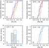 |
Fig. 7 Distribution of [Fe/H] for stars in NGC 6528. a) The black line shows the cummulative distribution of [Fe/H] for the full sample (21 stars). The orange-red line shows the distribution for stars where we have fitted the wings of Halpha to determine Teff (Method 2), while the purple line shows the distribution for the stars when we have used excitation equilibrium to determine Teff (Modified Method 2). b) The same as in a) but now only for stars with S/N> 35. c) The black line shows the histogram of [Fe/H] for stars in NGC 6528 for all stars with S/N> 35, while the blue line shows the result when the offset between the distributions for stars analysed with Method 2 and Modified Method 2 has been accounted for. d) The cummulative distribution of [Fe/H]. The colours are the same as in c). |
Unfortunately, the answer to the question posed in the headline of this section is – no. This should perhaps not come as a surprise, but given the results in Sect. 4.4 we would have expected that the results would be relatively similar and no (obvious) systematic differences present. This is, however, not the case.
Figure 7 shows the cumulative distributions of [Fe/H] for stars that are radial velocity members of NGC 6528. We plot the distribution for all stars, but also for stars analysed using Method 2 and Modified Method 2, respectively. Table 4 lists the number of stars in each sub-sample and the average [Fe/H]. Stars analysed using Method 2 are approximately 0.1 dex more metal-rich than stars analysed with Modified Method 2. The median is similarly off-set. We repeated the analysis on a subsection of the sample containing only the stars which have S/N> 35. Although this results in rather small samples the end-result remains (Fig. 7b).
We also note that when selecting only stars with S/N> 35 the full sample as well as the two sub-samples all give a lower [Fe/H] (by 0.03 dex). This agrees with what we found in the analysis of the noise injected spectra of Gaia benchmark stars (see Sects. 4.5 and 5.2).
To summarise, Fig. 6 indicate that the methods are very good at reproducing the final [Fe/H] also at relatively low S/N, but below about ~35 the errors increase and results in inflated values for [Fe/H]. However, of greater concern is that the results from the two methods are offset (Figs. 7a and b).
6. The metallicity of NGC 6528
6.1. Results
Given the results found in Sects. 5.2 and 5.3 defining the iron abundance of the metal-rich globular cluster NGC 6528 requires some care. In Method 2 the degeneracy between Teff and [Fe/H] is broken and is thus the most robust method to derive [Fe/H] with. Our final result for NGC 6528 will therefore be based on this method. In Fig. 7 (panels c and d) we show the final result when the [Fe/H] from Modified Method 2 are calibrated to Method 2 by applying the offset between the two methods to stars analysed with Modified Method 2.
The final sample of stars in NGC 6528 thus contains three (plus ten) stars with S/N> 35 (compare Table 4). If we consider these 13 stars which have S/N> 35 the mean and standard deviation change to + 0.04 dex with σ = 0.07 dex and hence an error in the derived mean abundance of 0.02 dex. This is our best estimate of [Fe/H] for NGC 6528.
Metallicity estimates for NGC 6528 using different samples.
6.2. Comparison with literature
The spectra of four red horizontal brach stars in NGC 6528 were analysed by Carretta et al. (2001). They found that the mean [Fe/H] for NGC 6528 is 0.07 ± 0.01 dex. Two of these stars (3014 and 3025) are part of our sample. For these stars our [Fe/H] are higher than found by Carretta et al. (2001). The difference is particularly large for 3014 for which our value is 0.1 dex higher. The discrepancy between the two results is mainly caused by the difference in Teff. Our Teff is hotter than that of Carretta et al. (2001) by about 150 K, while the log gs are similar.
Four of our stars (1-16, 1–24, 1-36, and 1-42) were taken from the sample by Zoccali et al. (2004). As discussed above, 1-24 is a spectroscopic binary and has been excluded from further analysis. Zoccali et al. (2004) note that 1-16 has a nearby companion. They therefore discarded also this star. As we have a large sample we are less worried about slight contamination of an individual spectrum and have kept the star in the sample.
The [Fe/H] determined by us and Zoccali et al. (2004) for 1-36 agree very well. On the other hand, the differences for I-42 are large. Although the two Teff are very similar, there is a difference in the metallicity and gravity of about 0.20 dex. Several possibilities might explain this discrepancy. The most obvious one being that we have different line lists and potentially also different log gf values for lines in comment6. We have also made use of the latest updates of log gf-values. We found that the uncertainty in the determined metallicity and gravity is much larger than the typical values, because 1-42 is a cooler giant (Teff ~ 4100 K). Zoccali et al. also found that 1-42 has large scatter in iron abundances. We also note that 1-42 has a lower S/N than the other stars from Zoccali et al. (2004). Given that it is also a cool giant and hence analysed with Modified Method 2, it is likely that the results are quite influenced by the deterioration in results below S/N ~ 35 (see also plots in Appendix E). Thus there does not seem to be one single issue that have contributed to the difference but several. Apart from these two high-resolution studies, several other recent studies are summarised in Table 5. Most of these agree with our results, with the exception of the metallicity derived from a comparison of the low resolution spectra to a grid of synthetic spectra (Coelho et al. 2001).
Metallicity estimates for NGC 6528 from the literature.
7. Conclusions and implications for the study of metal-rich stellar populations
With the aim of providing robust measures of [Fe/H] for metal-rich red giant branch stars we have conducted a thorough study of how best to analyse such spectra. We first analysed spectra for a set of so called benchmark stars to see which methods could best reproduce the reference values and secondly we analysed a set of spectra for a metal-rich globular cluster to appraise how well the chosen method fared in a real example with sometimes spectra of poor quality. Our conclusions are twofold. Firstly, low S/N in the spectra skews [Fe/H] values to higher values. Secondly, using excitation equilibrium to determine Teff results in [Fe/H] that are 0.1 dex lower than if we fit the wings of the Hα line are used to derive Teff.
These two effects should be taken into account when studying red giant stars in metal-rich stellar populations. In general the best approach would be to ensure large enough S/N in the spectra and only use stars with Teff> 4400 K. However, this might not always be practical or even possible. When cool stars need to be used or when the S/N on average can not be sufficiently high the study should implement a careful approach already at the telescope; a substantial number of warmer stars should be observed at sufficiently high S/N. These stars need not be part of the science sample, but can, for example, be stars in a globular cluster or in the field. In fact, stars in a globular cluster may be preferable as only there will it be straightforward to do the type of comparison that we present in Sect. 5.3
We study the [Fe/H] in the metal-rich and old globular cluster NGC 6528. We find that the most accurate value, taking the various issues summarised above into account, is [Fe/H] = + 0.04 dex with σ = 0.07 dex and hence an error in the derived mean abundance of 0.02 dex.
IRAF is distributed by the National Optical Astronomy Observatory, which is operated by the Association of Universities for Research in Astronomy (AURA) under cooperative agreement with the National Science Fundation.
In principle, other elements can also be used (e.g. Ti). However, there are only a few elements that have lines arising from both the neutral and singly ionised variety of the atom that are observable in the optical part of the spectrum. In those cases, often one of the ions has very few or very weak lines.
For these estimates we excluded the star HD 107328 as the [Fe/H] for that star is very different, and we do not have a straightforward answer to this discrepancy.
We can not make a comparison for the two list of iron lines, because Zoccali et al. did not publish their iron line data.
Acknowledgments
We thank an anonymous referee for his/her valuable comments and suggestions that have improved the paper. We thank Luca Sbordone who helped us to degrade the original Gaia benchmark star spectra to lower resolution and lower S/N. These degraded spectra were used in our tests.
This project was supported by the grant No. 621-2011-5042 from The Swedish Research Council. G.R. is funded by the project grant “The New Milky Way” from the Knut and Alice Wallenberg Foundation. This work has made use of the VALD database, operated at Uppsala University, the Institute of Astronomy RAS in Moscow, and the University of Vienna. This research made use of the SIMBAD database, operated at the CDS, Strasbourg, France.
References
- Adibekyan, V. Z., Sousa, S. G., Santos, N. C., et al. 2012, A&A, 545, A32 [NASA ADS] [CrossRef] [EDP Sciences] [Google Scholar]
- Adibekyan, V. Z., Figueira, P., Santos, N. C., et al. 2013, A&A, 554, A44 [NASA ADS] [CrossRef] [EDP Sciences] [Google Scholar]
- Aldenius, M., Lundberg, H., & Blackwell-Whitehead, R. 2009, A&A, 502, 989 [NASA ADS] [CrossRef] [EDP Sciences] [Google Scholar]
- Aurière, M. 2003, in EAS Pub. Ser. 9, eds. J. Arnaud, & N. Meunier, 105 [Google Scholar]
- Ballester, P., Modigliani, A., Boitquin, O., et al. 2000, The Messenger, 101, 31 [NASA ADS] [Google Scholar]
- Barklem, P. S., Stempels, H. C., Allen de Prieto, C., et al. 2002, A&A, 385, 951 [NASA ADS] [CrossRef] [EDP Sciences] [Google Scholar]
- Bensby, T., Feltzing, S., & Lundström, I. 2003, A&A, 410, 527 [NASA ADS] [CrossRef] [EDP Sciences] [Google Scholar]
- Bensby, T., Feltzing, S., & Lundström, I. 2004, A&A, 415, 155 [NASA ADS] [CrossRef] [EDP Sciences] [Google Scholar]
- Bensby, T., Yee, J. C., Feltzing, S., et al. 2013, A&A, 549, A147 [NASA ADS] [CrossRef] [EDP Sciences] [Google Scholar]
- Bensby, T., Feltzing, S., & Oey, M. S. 2014, A&A, 562, A71 [NASA ADS] [CrossRef] [EDP Sciences] [Google Scholar]
- Bergemann, M., Lind, K., Collet, R., Magic, Z., & Asplund, M. 2012, MNRAS, 427, 27 [NASA ADS] [CrossRef] [Google Scholar]
- Blanco-Cuaresma, S., Soubiran, C., Jofré, P., & Heiter, U. 2014, A&A, 566, A98 [NASA ADS] [CrossRef] [EDP Sciences] [Google Scholar]
- Bonnell, J. T., & Bell, R. A. 1993, MNRAS, 264, 334 [NASA ADS] [CrossRef] [Google Scholar]
- Brown, A. G. A. 2013, ArXiv e-prints [arXiv:1310.3485] [Google Scholar]
- Calamida, A., Bono, G., Lagioia, E. P., et al. 2014, A&A, 565, A8 [NASA ADS] [CrossRef] [EDP Sciences] [Google Scholar]
- Cardelli, J. A., Clayton, G. C., & Mathis, J. S. 1989, ApJ, 345, 245 [NASA ADS] [CrossRef] [Google Scholar]
- Carretta, E., Cohen, J. G., Gratton, R. G., & Behr, B. B. 2001, AJ, 122, 1469 [NASA ADS] [CrossRef] [Google Scholar]
- Coelho, P., Barbuy, B., Perrin, M.-N., et al. 2001, A&A, 376, 136 [NASA ADS] [CrossRef] [EDP Sciences] [Google Scholar]
- Cutri, R. M., Skrutskie, M. F., van Dyk, S., et al. 2003, 2MASS All Sky Catalog of point sources [Google Scholar]
- Dalton, G., Trager, S., Abrams, D. C., et al. 2014, in SPIE Conf. Ser., 9147, 91470 [Google Scholar]
- de Jong, R. S., Barden, S., Bellido-Tirado, O., et al. 2014, in SPIE Conf. Ser., 9147, 91470 [Google Scholar]
- Dekker, H., D’Odorico, S., Kaufer, A., Delabre, B., & Kotzlowski, H. 2000, in SPIE Conf. Ser. 4008, eds. M. Iye, & A. F. Moorwood, 534 [Google Scholar]
- Den Hartog, E. A., Ruffoni, M. P., Lawler, J. E., et al. 2014, ApJS, 215, 23 [NASA ADS] [CrossRef] [Google Scholar]
- Drake, J. J. 1991, MNRAS, 251, 369 [NASA ADS] [CrossRef] [Google Scholar]
- Drake, J. J., & Smith, G. 1991, MNRAS, 250, 89 [NASA ADS] [Google Scholar]
- Edvardsson, B. 1988, A&A, 190, 148 [NASA ADS] [Google Scholar]
- Edvardsson, B., Andersen, J., Gustafsson, B., et al. 1993, A&A, 275, 101 [NASA ADS] [Google Scholar]
- Feltzing, S., & Johnson, R. A. 2002, A&A, 385, 67 [NASA ADS] [CrossRef] [EDP Sciences] [Google Scholar]
- Feltzing, S., Primas, F., & Johnson, R. A. 2009, A&A, 493, 913 [NASA ADS] [CrossRef] [EDP Sciences] [Google Scholar]
- Fuhrmann, K. 1998, A&A, 338, 161 [NASA ADS] [Google Scholar]
- Fuhrmann, K. 2011, MNRAS, 414, 2893 [NASA ADS] [CrossRef] [Google Scholar]
- Fuhrmann, K., Pfeiffer, M., Frank, C., Reetz, J., & Gehren, T. 1997, A&A, 323, 909 [NASA ADS] [Google Scholar]
- Fulbright, J. P., McWilliam, A., & Rich, R. M. 2006, ApJ, 636, 821 [NASA ADS] [CrossRef] [Google Scholar]
- Gilmore, G., Randich, S., Asplund, M., et al. 2012, The Messenger, 147, 25 [NASA ADS] [Google Scholar]
- Gonzalez, O. A., Rejkuba, M., Zoccali, M., Valenti, E., & Minniti, D. 2011, A&A, 534, A3 [NASA ADS] [CrossRef] [EDP Sciences] [Google Scholar]
- Gonzalez, O. A., Rejkuba, M., Zoccali, M., et al. 2012, A&A, 543, A13 [NASA ADS] [CrossRef] [EDP Sciences] [Google Scholar]
- González Hernández, J. I., & Bonifacio, P. 2009, A&A, 497, 497 [NASA ADS] [CrossRef] [EDP Sciences] [Google Scholar]
- Gray, D. F. 1994, PASP, 106, 1248 [NASA ADS] [CrossRef] [Google Scholar]
- Gray, D. F. 2005, The Observation and Analysis of Stellar Photospheres (UK: Cambridge University Press) [Google Scholar]
- Gustafsson, B., Edvardsson, B., Eriksson, K., et al. 2008, A&A, 486, 951 [NASA ADS] [CrossRef] [EDP Sciences] [Google Scholar]
- Harris, W. E. 1996, AJ, 112, 1487 [NASA ADS] [CrossRef] [Google Scholar]
- Heiter, U., Jofré, P., Gustafsson, B., et al. 2015a, A&A, 582, A49 [NASA ADS] [CrossRef] [EDP Sciences] [PubMed] [Google Scholar]
- Heiter, U., Lind, K., Asplund, M., et al. 2015b, Phys. Scr., 90, 054010 [Google Scholar]
- Jofré, P., Heiter, U., Soubiran, C., et al. 2014, A&A, 564, A133 [NASA ADS] [CrossRef] [EDP Sciences] [Google Scholar]
- Jönsson, H., Ryde, N., Nordlander, T., et al. 2017, A&A, 598, A100 [NASA ADS] [CrossRef] [EDP Sciences] [Google Scholar]
- Kovtyukh, V. V., & Gorlova, N. I. 2000, A&A, 358, 587 [NASA ADS] [Google Scholar]
- Kupka, F., Piskunov, N., Ryabchikova, T. A., Stempels, H. C., & Weiss, W. W. 1999, A&AS, 138, 119 [NASA ADS] [CrossRef] [EDP Sciences] [MathSciNet] [PubMed] [Google Scholar]
- Kupka, F. G., Ryabchikova, T. A., Piskunov, N. E., Stempels, H. C., & Weiss, W. W. 2000, Balt. Astron., 9, 590 [NASA ADS] [Google Scholar]
- Mashonkina, L., Gehren, T., Shi, J.-R., Korn, A. J., & Grupp, F. 2011, A&A, 528, A87 [NASA ADS] [CrossRef] [EDP Sciences] [Google Scholar]
- Mayor, M., Pepe, F., Queloz, D., et al. 2003, The Messenger, 114, 20 [NASA ADS] [Google Scholar]
- McWilliam, A., Preston, G. W., Sneden, C., & Shectman, S. 1995, AJ, 109, 2736 [NASA ADS] [CrossRef] [Google Scholar]
- Meléndez, J., & Barbuy, B. 2009, A&A, 497, 611 [NASA ADS] [CrossRef] [EDP Sciences] [Google Scholar]
- Minniti, D., Lucas, P. W., Emerson, J. P., et al. 2010, New Astron., 15, 433 [NASA ADS] [CrossRef] [Google Scholar]
- Momany, Y., Ortolani, S., Held, E. V., et al. 2003, A&A, 402, 607 [NASA ADS] [CrossRef] [EDP Sciences] [Google Scholar]
- Origlia, L., Ferraro, F. R., Fusi Pecci, F., & Oliva, E. 1997, A&A, 321, 859 [NASA ADS] [Google Scholar]
- Origlia, L., Valenti, E., Rich, R. M., & Ferraro, F. R. 2005, MNRAS, 363, 897 [NASA ADS] [CrossRef] [Google Scholar]
- Pasquini, L., Avila, G., Blecha, A., et al. 2002, The Messenger, 110, 1 [NASA ADS] [Google Scholar]
- Perryman, M. A. C., Lindegren, L., Kovalevsky, J., et al. 1997, A&A, 323 [Google Scholar]
- Perryman, M. A. C., de Boer, K. S., Gilmore, G., et al. 2001, A&A, 369, 339 [NASA ADS] [CrossRef] [EDP Sciences] [Google Scholar]
- Pryor, C., & Meylan, G. 1993, in Structure and Dynamics of Globular Clusters, eds. S. G. Djorgovski, & G. Meylan, ASP Conf. Ser., 50, 357 [Google Scholar]
- Raassen, A. J. J., & Uylings, P. H. M. 1998, A&A, 340, 300 [NASA ADS] [Google Scholar]
- Ruchti, G. R., Bergemann, M., Serenelli, A., Casagrande, L., & Lind, K. 2013, MNRAS, 429, 126 [NASA ADS] [CrossRef] [Google Scholar]
- Simmerer, J., Feltzing, S., & Primas, F. 2013, A&A, 556, A58 [NASA ADS] [CrossRef] [EDP Sciences] [Google Scholar]
- Smith, G., & Raggett, D. S. J. 1981, J. Phys. B At. Mol. Phys., 14, 4015 [NASA ADS] [CrossRef] [Google Scholar]
- Soubiran, C., & Girard, P. 2005, A&A, 438, 139 [NASA ADS] [CrossRef] [EDP Sciences] [Google Scholar]
- Sozzetti, A., Torres, G., Charbonneau, D., et al. 2007, ApJ, 664, 1190 [NASA ADS] [CrossRef] [Google Scholar]
- Thévenin, F., & Idiart, T. P. 1999, ApJ, 521, 753 [NASA ADS] [CrossRef] [Google Scholar]
- Tsantaki, M., Sousa, S. G., Adibekyan, V. Z., et al. 2013, A&A, 555, A150 [NASA ADS] [CrossRef] [EDP Sciences] [Google Scholar]
- Valenti, J. A., & Fischer, D. A. 2005, ApJS, 159, 141 [NASA ADS] [CrossRef] [MathSciNet] [Google Scholar]
- Valenti, J. A., & Piskunov, N. 1996, A&AS, 118, 595 [NASA ADS] [CrossRef] [EDP Sciences] [Google Scholar]
- Vogt, S. S., Allen, S. L., Bigelow, B. C., et al. 1994, in Instrumentation in Astronomy VIII, eds. D. L. Crawford, & E. R. Craine, SPIE Conf. Ser., 2198, 362 [Google Scholar]
- Zoccali, M., Renzini, A., Ortolani, S., Bica, E., & Barbuy, B. 2001, AJ, 121, 2638 [NASA ADS] [CrossRef] [Google Scholar]
- Zoccali, M., Barbuy, B., Hill, V., et al. 2004, A&A, 423, 507 [NASA ADS] [CrossRef] [EDP Sciences] [Google Scholar]
Appendix A: NGC 6528 – a finding chart
Figure A.1 shows a finding chart centred on the field of the globular cluster NGC 6528. All stars from Table A.1 are marked (two stars fall outside the image) and identified by the number that is
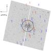 |
Fig. A.1 Image of the globular cluster NGC 6528 with the positions of stars we have analysed in this study marked. The stars are identified by the numbers listed in the first column in Table A.1. Red circles indicate stars observed with UVES, blue circles indicate stars observed with FLAMES-UVES, and black circles indicate stars observed with HIRES. The numbers next to the circles refer to the numbers in Table A.1. The core radius of the cluster (0.13 arcmin) is indicated by a red dashed line and the half-light (0.38 arcmin) by a black solid line. Data taken from Harris (1996). The image has been smoothed with a Gaussian to roughly mimic the seeing at Paranal. |
listed in the first column in Table A.1. The image is based on WFC3 observations with the HST and has been retrieved from the Mikulski Archive for Space Telescopes7.
Basic information for all stars analysed in this study.
Appendix B: Linelist
This section presents the full linelist used in the study of the ten Gaia benchmark stars and the red giant branch stars in NGC 6528. The data is shown in Table B.1, where references to the original sources of the data are also given. Most of the lines have been included in the linelist used in the Gaia-ESO Survey (Gilmore et al. 2012; Heiter et al., in prep.).
In the fourth column in Table B.1 we give the classification used in the Gaia-ESO linelist. Two flags are given, the left refers to the quality of the log gf and the second to the blending properties of the line.
• The flags have the following meaning for log gf:
-
y – Data come from a trusted source (mainly laboratorymeasurements with excellent accuracy).
-
u – Quality of data is not decided (advanced theoretical calculations and lower accuracy laboratory data).
-
n – Data are expected to have low accuracy.
• The flags have the following meaning for blending properties as assessed in spectra of the Sun and Arcturus:
-
y – Line is particularly un-blended or only blended with line ofsame species in both stars.
-
u – Line may be inappropriate in at least one of the stars.
-
n – Line is strongly blended with line(s) of different species in both the Sun and Arcturus.
Atomic line data.
Appendix C: Fitting of the wings of the Hα line to derive Teff
In this study we have fitted the wings of the Hα line by eye. We chose this approach in order to gain a deeper understanding of the issues facing the analysis of this line in the spectra of metal-rich giant stars. However, for larger samples and for a more routine approach an automated method should be attempted.
Figure C.1 shows our fits for three benchmark stars with different Teff (see the Figure caption). The warmest star is shown on top. This figure nicely illustrates the fact that the wings of the Hα line become less and less well developed in stars with cooler and cooler temperatures. Eventually, the wings become sufficiently weak that it is impossible to determine Teff from them.
Ideally, automated routines for fitting the wings should be used. This is not yet well explored for metal-rich stars such as
those in NGC 6528. It should be possible to adapt methods such as those in Barklem et al. (2002), but it might become increasingly difficult to define suitable windows to fit the spectra in metal-rich red giant stars. Figure C.1 shows the fits for three of the benchmark stars. As we performed the fits by hand we were able to customise the fitting regions. An experienced researcher may decide on different windows for the different spectra (as in our case). However, it would be feasible to stick to a single set of windows with these high quality spectra. This is more difficult when the spectra have low S/N. Figure C.2 shows how difficult it is to find clean regions in spectra with relatively low S/N. The spectrum shown in the top panel has a S/N of 29 and the one in the bottom panel has a S/N of 46. The two stars both have Teff> 4400 K, that is, we would expect to be able to fit the Hα line for both stars.
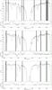 |
Fig. C.1 Comparison of synthetic spectra with the wings of Hα for the Gaia benchmark star ϵVir (Teff = 5056 K and log g = 2.8 dex), ξHya (Teff = 4991 K and log g = 2.96), and HD 107328 (Teff = 4483 K and log g = 2.0 dex). The middle synthetic spectrum (in red colour) is the best fit to the Hα wings, and the other two synthetic spectra indicate the shape of the wings when Teff is changed according to our estimated uncertainty. The marked grey regions were used to evaluate the goodness of the fit. We note that these are relatively short since many of the spectra have very little clean “line continuum” as a result of the cool temperatures which results in many molecular lines being present in the spectra. |
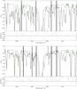 |
Fig. C.2 Comparison of synthetic spectra with the wings of Hα two stars in NGC 6528. Star-06 (Teff = 4623 K and log g = 1.98 dex) and Star-07 (Teff = 4776 K and log g = 2.50 dex). The middle synthetic spectrum (in red colour) is the best fit to the Hα wings, and the other two synthetic spectra indicate the shape of the wings when Teff is changed according to our estimated uncertainty. The marked grey regions were used to evaluate the goodness of the fit. We note the richer and more noisy spectra for these stars as compared to the benchmark stars displayed in Fig. C.1. |
Appendix D: Surface gravity from the three Ca i lines at 612.22, 616.22, and 643.91 nm
In Method 2 and Modified Method 2 (Sect. 4.3.2) we fitted the three strong Ca i lines at 612.22, 616.22, and 643.91 nm simultaneously to determine log g. This is not necessarily the only way to make use of the gravity sensitivity of these three lines. For example, it would be possible to fit each of the lines individually and take the average of the three determinations. Such an approach would also offer the possibility of deriving the scatter around the mean value as well as the error in the mean. In Table D.1 we report such results for the ten benchmark stars we have studied.
We find that for most stars, the typical uncertainty is around 0.10 dex. But, the determined log g suffers from a larger uncertainty for a lower gravity star. Except for βAra, the average of the three measured gravities (log gave) agree well with the obtained gravity (log gmethod2) by fitting the three Ca lines simultaneously listed in Table D.1. It is clearly shown that the determined log gmethod2 is strongly weighted by the second Ca line as log g from the Ca i 616.2 nm line is much larger than the other two lines.
Surface gravities measured from the strong Ca i lines.
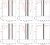 |
Fig. D.1 Comparison of synthetic spectra fitted to the wings of the three strong Ca i lines for two stars in NGC 6528. Star-05 (Teff = 4277 K and log g = 1.95 dex) and Star-07 (Teff = 4776 K and log g = 2.50 dex). The observed spectrum is indicated with a dotted line. The fitted spectrum is shown in red. This is the best fit as evaluated inside SME using the exact regions indicated with grey shaded regions. All three lines are fitted simultaneously, as implemented in Method 2. In the lower panels the residuals are shown. |
Appendix E: Exploration of impact of S/N on determination on stellar parameters for cool, metal-rich giant stars
As discussed in Sects. 4.5 and 5.2 the S/N of the spectra influences the results, at least for low S/N. This is one of the major findings of this study.
For several of the stars in NGC 6528 we have multiple exposures. This allows us to analyse spectra of different S/N for the same star. Using Method 2 and Modified Method 2 we analysed the spectra of five stars (Star-05, -07, -62, -65 and -67, IDs as in Table A.1). Figures 6 and E.1 show the results of our investigation. As a reference value we used the final parameters determined for each star, Table 3. The results shown for [Fe/H] were used to create Fig. 6.
It is easily seen, as expected, that when we analyse spectra of lower and lower S/N the scatter increases for all three parameters. It is in particular acute for log g which blows up to a rather large error quickly as the S/N deteriorates.
For Teff there is a marked increase in scatter and different stars appear, perhaps to behave in different ways. It is particularly interesting to compare and contrast star-62 and star-71. For star-71 (with Teff of 4560 K, thus analysed with Method 2) we systematically underproduce Teff when we go to lower S/N, while the opposite is true for star-62 (with Teff of 3967 K, thus analysed with Modified Method 2). For Teff there is thus a difference between Method 2 and Modified Method 2. We recall that Method 2 uses the wings of the Hα line to obtain Teff whilst Modified Method 2 uses excitation equilibrium of Fe i lines as the Hα wings disappear. Figure E.1 shows the detailed results.
The results for [Fe/H] are discussed in detail in the main body of the paper.
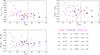 |
Fig. E.1 Comparison of the derived stellar parameters as a function of S/N. The y-axes show the difference between the value for each parameter derived from the low S/N spectrum and the value derived from the final combined spectrum (i.e. that used in the analysis in Sect. 6. The stellar parameters of the five stars are given in the legend. The colours (indicated in the legend) refer to how many spectra have been combined to obtain the analysed spectrum. |
All Tables
All Figures
|
Fig. 1 Comparison of radial velocities for the stars derived from the combined spectrum and from the individual spectra separately and then averaged (see Sect. 2.2.3). The x-axis shows the value derived from the combined spectra whilst the y-axis shows the difference between vr determined in the two ways. The error-bars for the difference is the coadded errors estimated from IRAF (for the combined spectra) and the σ around the mean for the independent measures. Errors on the x-axis are too small to be seen. |
| In the text | |
|
Fig. 2 Distribution of measured heliocentric radial velocities for our programme stars. The inset in the top-left corner shows a zoom-in high-lighting the velocity distribution of the cluster members fitted by a Gaussian. The red cross indicates the mean (212.1 km s-1) and standard deviation (4.2 km s-1) of the radial velocity for the cluster members. |
| In the text | |
|
Fig. 3 Test of the ability of our linelist to reproduce the reference [Fe/H] for the Gaia benchmark stars. The y-axis shows the difference between the reference value and the value we derive (using the reference Teff and log g, but our own linelist and SME). We derived [Fe/H] in three ways: using both Fe i and Fe ii lines (blue filled squares), using only Fe i lines (red filled circles), and using only Fe ii lines (black filled triangles). The stars can be identified using the Teff values which are given on the x-axis. For some of the stars we have more than one spectrum. Results for both are shown in the plot. |
| In the text | |
|
Fig. 4 Comparison of synthetic spectra with the wings of Hα line in ϵVir. The middle synthetic spectrum (in red) shows the best fit. The other two synthetic spectra (blue and green) indicate the shape of the wings when Teff is changed according to our estimated uncertainty (here 50 K). The grey areas mark the regions used to evaluate the goodness of the fit. Note that these are relatively narrow since the spectrum has very little clean “line continuum” thanks to the cool temperature of the star, which results in many lines being present in the spectrum. |
| In the text | |
|
Fig. 5 Comparison of the stellar parameters derived using the three methods discussed in Sects. 4.3.1 till 4.3.3 with the reference values (Table 2). On each y-axis is indicated the difference between the values we have obtained and the reference value (indicated by a subscript “r”). Method 1 is indicated by red symbols, Method 2 by black, and Method 3 is indicated by cyan symbols. Different symbols represent the different stars (as indicated in the figure, note that each symbol represent two stars. They should be easy to identify thanks to their different Teff). Note that some stars have more than one spectrum analysed (see Sect. 2.1.1). The stars can be identified by their recommended Teff which is plotted on the x-axis. The dashed line indicates the separation of “cool” (left) and “warm” (right) giants (see Sect. 4.3.2). |
| In the text | |
|
Fig. 6 Difference between [Fe/H] derived from spectra of varying S/N (per pixel) for stars in NGC 6528. [Fe/H]x indicates our value measured for each spectrum, while [Fe/H]r indicate the value obtained in Sect. 5.1 for each star. The full line indicated the average difference evaluated as a running average. The shaded region indicates the 1σ difference, while the dashed-dotted line indicates the 2σ difference. Details on individual stars are given in Appendix E. Note that in this figure we do not distinguish between stars for which different methods to derive Teff have been used (compare Fig.7). |
| In the text | |
|
Fig. 7 Distribution of [Fe/H] for stars in NGC 6528. a) The black line shows the cummulative distribution of [Fe/H] for the full sample (21 stars). The orange-red line shows the distribution for stars where we have fitted the wings of Halpha to determine Teff (Method 2), while the purple line shows the distribution for the stars when we have used excitation equilibrium to determine Teff (Modified Method 2). b) The same as in a) but now only for stars with S/N> 35. c) The black line shows the histogram of [Fe/H] for stars in NGC 6528 for all stars with S/N> 35, while the blue line shows the result when the offset between the distributions for stars analysed with Method 2 and Modified Method 2 has been accounted for. d) The cummulative distribution of [Fe/H]. The colours are the same as in c). |
| In the text | |
|
Fig. A.1 Image of the globular cluster NGC 6528 with the positions of stars we have analysed in this study marked. The stars are identified by the numbers listed in the first column in Table A.1. Red circles indicate stars observed with UVES, blue circles indicate stars observed with FLAMES-UVES, and black circles indicate stars observed with HIRES. The numbers next to the circles refer to the numbers in Table A.1. The core radius of the cluster (0.13 arcmin) is indicated by a red dashed line and the half-light (0.38 arcmin) by a black solid line. Data taken from Harris (1996). The image has been smoothed with a Gaussian to roughly mimic the seeing at Paranal. |
| In the text | |
|
Fig. C.1 Comparison of synthetic spectra with the wings of Hα for the Gaia benchmark star ϵVir (Teff = 5056 K and log g = 2.8 dex), ξHya (Teff = 4991 K and log g = 2.96), and HD 107328 (Teff = 4483 K and log g = 2.0 dex). The middle synthetic spectrum (in red colour) is the best fit to the Hα wings, and the other two synthetic spectra indicate the shape of the wings when Teff is changed according to our estimated uncertainty. The marked grey regions were used to evaluate the goodness of the fit. We note that these are relatively short since many of the spectra have very little clean “line continuum” as a result of the cool temperatures which results in many molecular lines being present in the spectra. |
| In the text | |
|
Fig. C.2 Comparison of synthetic spectra with the wings of Hα two stars in NGC 6528. Star-06 (Teff = 4623 K and log g = 1.98 dex) and Star-07 (Teff = 4776 K and log g = 2.50 dex). The middle synthetic spectrum (in red colour) is the best fit to the Hα wings, and the other two synthetic spectra indicate the shape of the wings when Teff is changed according to our estimated uncertainty. The marked grey regions were used to evaluate the goodness of the fit. We note the richer and more noisy spectra for these stars as compared to the benchmark stars displayed in Fig. C.1. |
| In the text | |
|
Fig. D.1 Comparison of synthetic spectra fitted to the wings of the three strong Ca i lines for two stars in NGC 6528. Star-05 (Teff = 4277 K and log g = 1.95 dex) and Star-07 (Teff = 4776 K and log g = 2.50 dex). The observed spectrum is indicated with a dotted line. The fitted spectrum is shown in red. This is the best fit as evaluated inside SME using the exact regions indicated with grey shaded regions. All three lines are fitted simultaneously, as implemented in Method 2. In the lower panels the residuals are shown. |
| In the text | |
|
Fig. E.1 Comparison of the derived stellar parameters as a function of S/N. The y-axes show the difference between the value for each parameter derived from the low S/N spectrum and the value derived from the final combined spectrum (i.e. that used in the analysis in Sect. 6. The stellar parameters of the five stars are given in the legend. The colours (indicated in the legend) refer to how many spectra have been combined to obtain the analysed spectrum. |
| In the text | |
Current usage metrics show cumulative count of Article Views (full-text article views including HTML views, PDF and ePub downloads, according to the available data) and Abstracts Views on Vision4Press platform.
Data correspond to usage on the plateform after 2015. The current usage metrics is available 48-96 hours after online publication and is updated daily on week days.
Initial download of the metrics may take a while.