| Issue |
A&A
Volume 600, April 2017
|
|
|---|---|---|
| Article Number | A10 | |
| Number of page(s) | 23 | |
| Section | Planets and planetary systems | |
| DOI | https://doi.org/10.1051/0004-6361/201629800 | |
| Published online | 20 March 2017 | |
Observing transiting planets with JWST
Prime targets and their synthetic spectral observations
1 Max-Planck-Institut für Astronomie, Königstuhl 17, 69117 Heidelberg, Germany
e-mail: This email address is being protected from spambots. You need JavaScript enabled to view it.
2 Irfu, CEA, Université Paris-Saclay, 9119 Gif-sur Yvette, France
3 AIM, Université Paris Diderot, 91191 Gif-sur-Yvette, France
4 SRON Netherlands Institute for Space Research, Sorbonnelaan 2, 3584 CA Utrecht, The Netherlands
5 Astronomical institute Anton Pannekoek, University of Amsterdam, Science Park 904, 1098 XH Amsterdam, The Netherlands
Received: 28 September 2016
Accepted: 21 November 2016
Abstract
Context. The James Webb Space Telescope will enable astronomers to obtain exoplanet spectra of unprecedented precision. The MIRI instrument especially may shed light on the nature of the cloud particles obscuring planetary transmission spectra in the optical and near-infrared.
Aims. We provide self-consistent atmospheric models and synthetic JWST observations for prime exoplanet targets in order to identify spectral regions of interest and estimate the number of transits needed to distinguish between model setups.
Methods. We select targets that span a wide range of planetary temperatures and surface gravities, ranging from super-Earths to giant planets, that have a high expected signal-to-noise ratio. For all targets, we vary the enrichment, C/O ratio, presence of optical absorbers (TiO/VO), and cloud treatment. We calculate atmospheric structures, emission, and transmission spectra for all targets and use a radiometric model to obtain simulated observations. Further, we analyze JWST’s ability to distinguish between various scenarios.
Results. We find that in very cloudy planets, such as GJ 1214b, less than ten transits with NIRSpec may be enough to reveal molecular features. Furthermore, the presence of small silicate grains in atmospheres of hot Jupiters may be detectable with a single JWST MIRI transit. For a more detailed characterization of such particles less than ten transits are necessary. Finally, we find that some of the hottest hot Jupiters are well fitted by models which neglect the redistribution of the insolation and harbor inversions, and that 1–4 eclipse measurements with NIRSpec are needed to distinguish between the inversion models.
Conclusions. Wet thus demonstrate the capabilities of JWST for solving some of the most intriguing puzzles in current exoplanet atmospheric research. Further, by publishing all models calculated for this study we enable the community to carry out similar studies, as well as retrieval analyses for all planets included in our target list.
Key words: methods: numerical / planets and satellites: atmospheres / radiative transfer
© ESO, 2017
1. Introduction
The James Webb Space Telescope (JWST), will be one of the most exciting instruments for exoplanet science in the years to come. It will be the first telescope to offer a continuous wavelength coverage from 0.6 to 28 μm (Beichman et al. 2014). Unaffected by telluric absorption, it will allow probing of the red optical part of a planetary spectrum (including the K-doublet line in hot Jupiters), the near-infrared (NIR) (including molecular transitions of water and methane) and the mid-infrared (MIR) part.
Observing exoplanet transit spectra in the MIR may be key (Wakeford & Sing 2015) to identifying cloud species which often weaken or even fully blanket the atomic and molecular features in the optical and NIR (see, e.g., GJ1214b (Kreidberg et al. 2014), HD 189733b Sing et al. 2011, WASP-6b Jordán et al. 2013; and WASP-12b Sing et al. 2013).
This claim for cloudiness has often been based on lacking or muted alkali absorption features and strong Rayleigh signatures in the optical part of hot Jupiter transmission spectra, or muted water features in the NIR. Additionally, entirely featureless transmission spectra (GJ 1214b) have been observed.
While it was theorized that muted water features could also be caused by depletion of water (Madhusudhan et al. 2014b), or a general depletion of metals in the atmospheres, evidence nowadays seems to point to the presence of clouds (Sing et al. 2015a; Iyer et al. 2016) or a combination of clouds and metal depletion (Barstow et al. 2017).
At the same time, the nature of these clouds is still unknown. Depending on the size of the cloud particles, their opacity in the optical and NIR transitions from a Rayleigh slope (small particles) to a flat, gray opacity (large particles). The resonance features of possible chemical equilibrium cloud species all lie in the MIR (Wakeford & Sing 2015) such that a distinction between cloud species may only be possible within the MIR region. The formation of clouds and hazes by non-equilibrium processes is another possibility, although hot Jupiters, especially, seem to be too hot for the “classical” case of hydrocarbon hazes (Liang et al. 2004) as well as for newly suggested pathways such as photolytic sulfur clouds (Zahnle et al. 2016).
The predicted data quality in combination with the wavelength coverage of JWST will enable exoplanet atmosphere characterization to a degree which is, using today’s observational facilities, impossible. The possible gain when having high quality MIR data can be seen when considering the pre-warm Spitzer spectrum for HD 189733b (from ~5–14 μm, see Grillmair et al. 2008; Todorov et al. 2014) and the increased capability to characterize this planet’s atmosphere using retrieval when compared to planets with sparse photometric data (Line et al. 2014).
While the question of the origins of clouds is fundamental and not yet answered, future efforts of characterizing planetary atmospheres will increasingly concentrate on the quantitative characterization of atmospheres. Using emission spectra, even the characterization of atmospheres appearing cloudy in transmission may well be possible, as is the case for HD 189733b (Barstow et al. 2014; Line et al. 2014). The reason for this is the clouds’ decreased optical depth when not being viewed in transit geometry (Fortney 2005). Moreover, the analysis of the resulting atmospheric composition and abundance ratios may allow placement of constraints on planets’ formation locations, although the exact interpretation of the atmospheric abundances depends on the assumptions and the degree of complexity of the model being used to describe the planet formation and evolution (Öberg et al. 2011; Ali-Dib et al. 2014; Thiabaud et al. 2014; Helling et al. 2014; Marboeuf et al. 2014b,a; Madhusudhan et al. 2014a, 2016; Mordasini et al. 2016; Öberg & Bergin 2016; Cridland et al. 2016).
As the launch of JWST (currently projected for October 2018) draws nearer, the exoplanet community is in increased need of predictions by both instrument and exoplanet models in order to maximize the scientific yield of observations. The actual performance of JWST will only be known once the telescope has been launched and the first observations have been analyzed (Stevenson et al. 2016b). Nonetheless, the modeling efforts of the telescope performance in conjunction with models of exoplanet atmospheres have already been started and include Deming et al. (2009), Batalha et al. (2015), Mordasini et al. (2016). Studies which additionally look into the question of retrievability of the atmospheric properties as a function of the planet-star parameters can be found Barstow et al. (2015), Greene et al. (2016), Barstow & Irwin (2016). Barstow et al. (2015) also included time-dependent astrophysical noise (starspots) for stitched observations.
In this study we present detailed self-consistent atmospheric model calculations for a set of exoplanets which we have identified as prime scientific targets for observations with JWST. The target selection was carried out considering the planets’ expected signal-to-noise ratio (S/N) for both transit and emission measurements, putting emphasis on a good S/N for observations with JWST’s MIRI instrument to allow measurements in the MIR. The planets uniformly cover the log (g)–Tequ parameter space which may also allow prediction of the objects’ cloudiness (Stevenson 2016). We calculate a suite of models for every candidate planet. We vary the planetary abundances by adopting different values for [Fe/H] and C/O, including very high enrichments (and high mean molecular weights) for super-Earth and Neptune-sized planets. For all planets, we additionally calculate models including clouds, setting the free parameters of the cloud model to produce either small or large cloud particles which we assume to be hollow spheres to mimic irregularly shaped dust aggregates. Alternatively, we assume a spherically-homogeneous shape. For the hottest target planets, TiO and VO opacities are optionally considered. The irradiation is treated as either assuming a dayside or global average of the received insolation flux. For some very hot planets we additionally calculate emission spectra neglecting any energy redistribution by winds.
For all target planets, we present synthetic emission and transmission spectral observations for the full JWST wavelength range and compare them to any existing observational data.
For conciseness we present an exemplary analysis for a subset of the targets considered in this paper. To this end, we select three specimens belonging to the classes of extemely cloudy super-Earths, intermediately irradiated gas giants, and extremely hot, strongly irradiated gas giants, respectively. We discuss how JWST may shed light on the nature of these planetary classes, by detecting molecular features in the NIR transmission spectra for cloudy super-Earths, or by identifying cloud resonance features in the MIR for hot Jupiters. For the hottest planets we study how well JWST can distinguish between various models which individually fit well to the data currently available.
For all targets, we publish the atmospheric structures, spectra, and simulated observations online. These results will facilitate prediction of the expected signal quality of existing prime exoplanet targets for JWST.
In Sect. 2 we describe the models used for carrying out our calculations, while in Sect. 3, the candidate selection criteria and target list are described. In Sect. 4 we describe which parameter setups were considered for all planets. This is followed by a characterization of the results in Sect. 5. Next, we analyze the synthetic observations of a selected subsample of targets in Sect. 6. Finally, we describe the extent and format of the data being published in Sect. 7 and describe our summary and conclusions in Sect. 8.
2. Modeling
2.1. Atmospheric model
The petitCODE calculates the atmosphere’s radiative-convective equilibrium structure in chemical equilibrium. The chemistry module includes condensation, delivers abundances for the gas opacities, and serves as an input for the cloud model. During the computation of the atmospheric equilibrium structures, scattering is included for solving the radiative transport equation. For a fully converged atmosphere, the code returns the atmospheric structure (such as temperature, molecular abundances, etc.) as well as the atmosphere’s emission and transmission spectrum at a resolution of λ/ Δλ = 1000, where Δλ is the size of a spectral bin.
Since the first version of the code described in Mollière et al. (2015), we have introduced several additions which lead to the current set of capabilities described above. These additions have been partially described in Mancini et al. (2016a,b), but in this work we provide a full description (see Appendix A).
Here we summarize the additions to the code:
-
Line cutoff: we now apply a sub-Lorentzian line treatment to allmolecular and atomic lines far away from the line center.
-
Chemistry: we now use a self-written Gibbs minimizer for the equilibrium chemistry, which reliably converges between 60–20 000 K and treats the condensation of 15 different species.
-
Clouds: we implemented the Ackerman & Marley (2001) cloud model, for which we introduce a new derivation in Appendix B, showing that the cloud model is independent of the microphysics of nucleation, condensation, coagulation, coalescence, and shattering as long as some underlying assumptions are fulfilled. The implementation of the cloud model is described in Appendix A. We treat mixing arising from convection, convective overshoot, and stellar irradiation.
-
Cloud opacities: for the clouds, we calculate particle opacities using the distribution of hollow spheres (DHS) or Mie theory. For this we use the code by Min et al. (2005). While Mie theory follows the classic assumption of spherical, homogeneous grains, DHS theory assumes a distribution of hollow spheres in order to approximate the optical properties of irregularly shaped dust aggregates. We consider clouds composed of MgAl2O4, Mg2SiO4, Fe, KCl and Na2S. In our model, clouds of different species cannot interact and are treated separately.
-
Transmission spectra can now be calculated.
-
The molecular opacity database has been updated to include Rayleigh scattering for H2, He, CO2, CO, CH4, and H2O. Additionally, we can optionally include TiO and VO opacities.
-
Scattering: we implemented scattering for both the stellar and planetary light, applying local accelerated lambda iteration (ALI; Olson et al. 1986) and Ng-acceleration (Ng 1974).
2.2. Radiometric model
We simulate JWST observations with the EclipseSim package (van Boekel et al. 2012). For this we consider observations in the NIRISS (Doyon et al. 2012), NIRSpec (Ferruit et al. 2012), and MIRI instruments (Wright et al. 2010). The length of each observation is taken to be the full eclipse duration, bracketed by “baseline” observations before and after the eclipse, which each have a duration of the eclipse itself.
For the synthetic observations, we assumed the instrumental resolution. If needed, these spectra can be re-binned to lower resolution. For the NIRISS slitless spectroscopy, the SOSS mode in first order is used. For NIRSpec, we assume the G395M mode and for MIRI, the LRS mode. Using these modes, one obtains a close to complete spectral coverage between 0.8 and 13.5 microns. However, since JWST can only observe in one instrument at a time, one needs three separate observations to obtain the complete spectral coverage.
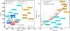 |
Fig. 1 Left panel: our transit candidates in log (g)–Tequ space. See the legend for the meaning of the symbols. Candidates with gray symbols are artificial and have been introduced to fill in the parameter space. “T” and “E” in the legend stand for planets which can be observed in transmission or emission, respectively. The vertical and horizontal lines separate the mostly cloud-free (upper right region) from the potentially cloudy atmospheres (left and bottom regions) as defined in Stevenson (2016). The black, orange, green, and magenta lines show log (g)–Tequ curves of super-Earths and Neptune-like planets (Lopez & Fortney 2014) for the masses and envelope mass fractions as described in the legend. The giant planets which have a gray frame around their name box are not inflated. The upper ends of the vertical orange lines shown for Kepler-13Ab and WASP-18b denote the maximum brightness temperatures observed for these planets. Right panel: planetary mean density as a function of mass. Only the giant planet candidates are plotted here, in the same style as in the left panel. A sample of synthetic, non-inflated planets calculated using the model of Mordasini et al. (2012), Alibert et al. (2013), Jin et al. (2014) is shown as gray crosses. The value of the straight red line shown in the model is a linear function of the planetary mass, as is expected for non-inflated giant planets (see, e.g., Baruteau et al. 2016). |
3. Candidate selection
3.1. Candidate selection criteria
In order to obtain a list of well observable candidates, we only considered planets for which the transit times are known accurately. As an additional criterion, we checked if a candidate is observable in transmission and/or emission with signal amplitude (at 7 μm) of S/N > 5, where the noise is assumed to be photon noise + a 50 ppm noise floor. For this initial check we approximated the planetary emission using a blackbody spectrum, whereas for the transmission signal we assumed a transit signal amplitude of five pressure scale heights.
This initial analysis results in a large number of possible targets, given the wealth of transiting exoplanets known already today. In order to maximize the scientific yield of the first JWST observations, it may be instructive to first observe a planetary sample as diverse as possible and to embark on more detailed studies within a given planetary class later on. Our goal, therefore, is to define such a diverse target list, and to map out the parameter space defining planetary classes as well as possible.
The main physical parameter space for candidate selection in the work presented here is the log (g)–Tequ space. This space is quite fundamental in the sense that the equilibrium temperature and the planetary surface gravity are two key parameters impacting the pressure temperature structure and spectral appearance of a planet (see, e.g., Sudarsky et al. 2003; Mollière et al. 2015). The total atmospheric enrichment can be of importance too, but for scaled solar compositions, variations of log (g) and [Fe/H] are degenerate to some degree (Mollière et al. 2015). Additionally, for every target planet, we present calculations assuming a larger or smaller enrichment than used in the fiducial case. Further, a planet’s location in the log (g)–Tequ space may allow to assess if the planet is cloudy or not (see Stevenson 2016). We aimed for a broad coverage of candidates in our parameter space.
In addition, we divided the candidates into super-Earths, hot Neptunes, and inflated and non-inflated giant planets and tried to select a sample as diverse as possible, still above observational thresholds described above, however.
Our final selection is shown in the left panel of Fig. 1. For the super-Earths and hot Neptunes, we only have four candidates in total, two for each class. In order to estimate the region usually occupied by these two classes of planets, we overplot log (g)–Tequ lines for super-Earths and hot Neptunes of varying mass and envelope fraction (taken from Lopez & Fortney 2014) to investigate the area that super-Earths and Neptunes may occupy in log (g)–Tequ space. We added two more hot, artificial candidates, one for the Neptunes and one for the super-Earths, to increase the coverage in log (g)–Tequ space. We cannot introduce even hotter artificial super-Earths or Neptunes, because their envelopes would likely be evaporated (Jin et al. 2014).
The giant planets were divided into inflated giant planets, non-inflated giant planets, and inflated giant planets associated to non-inflated giant planets. This association means that the inflated planets are lying close to the non-inflated ones in log (g)–Tequ space, but are inflated. It is known that whether or not inflation occurs is correlated to irradiation strength and thus Tequ (Laughlin et al. 2011; Demory & Seager 2011). Therefore, such close neighbors in log (g)–Tequ space, showing inflation or no inflation, may potentially shed light on the mechanisms driving inflation. To assess whether or not a giant planet is inflated, we show the density of all candidates as a function of their mass in the right panel of Fig. 1. We also plot a synthetic planetary population, calculated using the planet formation and evolution code of Mordasini et al. (2012), Alibert et al. (2013), Jin et al. (2014), which does not include any inflation processes. All planets that have a density lower than the one shown for the synthetic giant planets were considered to be inflated.
3.2. List of selected candidates
The parameters of the exoplanet targets modeled in this paper are given in Table 1.
For the super-Earths we included a planet with a mass of 5 M⊕, placed at a distance of 0.1 AU around a Sun-like star, which corresponds to a planetary equilibrium temperature of 880 K. We assumed an initial H–He envelope mass fraction of 1% of the planet’s total mass. Calculations by Jin et al. (2014) indicate that such a planet loses approximately half of its envelope in the first 20 Myr of its lifetime, therefore we calculate the radius of the planet using the relation by Lopez & Fortney (2014) for a 5 M⊕ planet with a 0.5% envelope fraction at an age of 20 Myr. At later times, the envelope of such a planet will be evaporated even further, therefore the high enrichment we assume for its atmosphere (see Sect. 4) may be seen as a proxy for a secondary atmosphere with a high mean molecular weight. Note that photo-evaporation is not included in the calculations of Lopez & Fortney (2014). We refrained from considering even hotter super Earth planets, because more strongly irradiated planets will be more strongly affected by photo-evaporation such that the primordial planetary H–He envelope may not survive.
For the Neptunes, we considered an artificial object with a mass of 20 M⊕ in orbit around a Sun-like star with a semi-major axis of 0.05 AU, corresponding to an effective temperature of 1250 K. The H–He envelope mass fraction was taken to be 15%. Again, we consulted Jin et al. (2014) and found that such a planet may retain a significant amount of its envelope up to 100 Myr and longer.
The parameters for the artificial planets listed in Table 1 were again obtained using Lopez & Fortney (2014).
High priority targets for which we simulate spectra in this study.
4. Selection of planet parameters
For every target identified in Sect. 3.2, and modeled in Sect. 5, we calculate a fiducial model, and then vary five parameters within a parameter space, which we will describe in the following. The parameters that are studied are the atmospheric enrichment (see Sect. 4.1), clouds (Sect. 4.2), the C/O number ratio (Sect. 4.3), the inclusion of optical absorbers in the form of TiO/VO (Sect. 4.4), and the redistribution of the stellar irradiation energy (Sect. 4.5).
4.1. Atmospheric enrichment
The analysis of the radii of known, cool (Tequ< 1000 K) exoplanets using planetary structure models suggests that the planets’ enrichment in heavy elements, ZPl, is proportional to the host stars’ metal enrichment Z∗. The ratio ZPl/Z∗ is a function of the planetary mass and decreases with increasing planetary mass (Miller & Fortney 2011; Thorngren et al. 2016). A fit of the function, 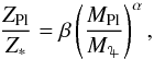 (1)to the sample of planets investigated in Miller & Fortney (2011) yields α = −0.71 ± 0.10 and β = 6.3 ± 1.0 (Mordasini et al. 2014). In the same paper, (Mordasini et al. 2014) fit the results of a synthetic population of planets formed via the core accretion paradigm and find α = −0.68 and β = 7.2, which fits the observational data and the Solar System ice and gas giants. A comprehensive summary of observational evidence further backing the finding that lower-mass planets are more heavily enriched than more massive planets can be found in Mordasini et al. (2016).
An important question asks to what extent the metal content of the planet is mixed into its envelope and atmosphere. It is suggested that for Saturn, nearly all metals are locked into the central core, whereas for Jupiter the metals appear to be fully mixed into the envelope (Fortney & Nettelmann 2010). In our fiducial models, we assume planets where half of the metal enrichment is mixed into the planet’s envelope and atmosphere.
For the fiducial models of the planets whose atmospheres we will simulate, we thus use Eq. (1) to describe the atmospheric enrichment, taking into account an additional factor 1/2 to relate the atmospheric enrichment to the planetary bulk enrichment. We take the host star’s [Fe/H] as a proxy for the stellar enrichment.
Additionally, we consider models with ten times more or less metal enrichment than in the fiducial model.
4.2. Clouds
For every planet we consider nine different cloud model parameter setups in order to test a broad range of possible cloud properties. These setups are listed in Table 2.
Models 1 and 2 use the Ackerman & Marley (2001) cloud model to couple the effect of clouds self-consistently with the atmospheric temperature iteration. The values for the settling parameter fsed, which is the ratio of the mass averaged grain settling velocity and the atmospheric mixing velocity, have been adopted covering the lower range of what is typically being used for brown dwarfs (fsed = 1–5, see Saumon & Marley 2008; Morley et al. 2012) and we use fsed = 1,3 here. Further, we account for the fact that Earth’s high altitude clouds are well described using small fsed< 1 values, and that the flat transmission spectrum of GJ 1214b is best described using fsed ≪ 1 (Ackerman & Marley 2001; Morley et al. 2013, 2015). We therefore use such small fsed value cloud setups in models 3 and 4, namely fsed = 0.3 and 0.01. Similar to Morley et al. (2015), we find that for the cases with small fsed< 1, with the planets often being quite strongly enriched, it can be challenging to obtain converged results when self-consistently coupling the cloud model to the radiative-convective temperature iteration. Thus, for cloud model setups 3 and 4, we follow a two-pronged approach: first, we attempt to calculate the atmospheric structures self-consistently, and if this does not succeed we follow Morley et al. (2015) and calculate cloudy spectra for these two model setups using the temperature structure of the fiducial, cloud-free model.
For the cases where the cloud models 3 and 4 converged, and for all other cloud models considered here, the clouds are coupled to the atmospheric structure iteration self-consistently. For, GJ 1214b, for example, which has an enrichment of 1000 × solarin our fiducial setup, the structures for cloud models 3 and 4 with self-consistent coupling converged. We look at this planet in greater detail in Sect. 6.1.1. For cases for which the self-consistent coupling between cloud models 3 and 4 and the temperature iteration converged, we compared the resulting spectra to the calculations which applied models 3 and 4 to the cloud-free temperature structure. We found that the transmission spectra can agree quite well but may be offset due to different temperatures in the atmospheres. If the atmospheric temperatures are close to a chemically important temperature range (e.g. close to the temperature where carbon gets converted from methane (lower temperatures) to CO (larger temperatures)), the transmission spectra can be quite different, with the cooler, not self-consistently coupled atmospheres exhibiting methane features which the self-consistent atmospheres lack. Analogously, emission spectra may share a similar spectral shape (not in all cases, due to the same reasons as outlined above for transmission spectra) but have a different flux normalization: the self-consistent models 3 and 4 conserve the flux, while the post-processed cloud calculations, simply applying clouds to the clear atmospheric structures for the spectra, do not.
We want to stress that our implementation of the Ackerman & Marley (2001) cloud model differs from the version described in the original paper in two ways: (i) we account for vertical mixing induced by insolation (see Appendix A.3). A similar approach was taken for GJ 1214b in the study by Morley et al. (2015) and (ii) the mixing length in our cloud model implementation is equal to the atmospheric pressure scale height, while in the Ackerman & Marley (2001) model the mixing length in the radiative layers is up to ten times smaller than the atmospheric pressure scale height. This means that for a given fsed value, our clouds will be more extended, because the cloud density above the cloud deck is proportional to Pfsed/λ, where λ is the ratio of the mixing length L divided by the pressure scale height H. Further, the mixing velocity is equal to Kzz/L, where Kzz is the atmospheric eddy diffusion coefficient, meaning that for a given fsed value, our grains will be smaller. Both effects effectively lower our fsed value in comparison to the Ackerman & Marley (2001) value. See Appendix A.3 for a description of our implementation of the Ackerman & Marley (2001) cloud model.
In our standard case, the cloud particles are assumed to be irregularly shaped dust aggregates, which we describe using the Distribution of Hollow Spheres method (DHS). This is in contrast to the case of homogeneous spheres in Mie theory. We investigate the effect of Mie opacities as a non-standard scenario in cloud model 9. Only the small cloud particle case is studied with Mie theory, as only then may differences between DHS and Mie in the cloud resonance features be seen: for larger particles the cloud opacity is gray for both the DHS and Mie treatment, without any observable features.
So far, the use of Mie theory is a standard approach for cloud particles in brown dwarf/exoplanet atmospheres (see, e.g., Helling et al. 2008; Madhusudhan et al. 2011a; Morley et al. 2012; Benneke 2015; Baudino et al. 2015), which is a useful starting point to assess the first-order effect of clouds on planetary structures and spectra. However, in all cases where crystalline features of silicate grains have been observed in an astrophysical context so far, it was found that the opacity of Mie grains poorly fits the observations. Only the use of non-homogeneous or non-spherical shapes, such as DHS or Continuous Distribution of Ellipsoids (CDE), provides a good fit to the data. Examples are the features of dust particles in disks around Herbig Ae/Be stars (Bouwman et al. 2001; Juhász et al. 2010), as well as AGB stars, post-AGB stars, planetary nebulae, massive stars, but also stars with poorly known evolutionary status (for a discussion of the data and the spectral fits see Molster et al. 2002; Min et al. 2003, respectively). Given the observational evidence in different astrophysical scenarios, we therefore chose the DHS treatment of grains as our standard scenario. We note that for brown dwarfs, an explicit detection of a cloud feature is still missing (although tentative evidence exists, see Cushing et al. 2006) and that transmission spectra of planets have so far only probed the (often cloudy/hazy) optical and NIR regions, which are devoid of cloud resonance features because these lie primarily in the MIR.
For models 5 to 9 in Table 2, we introduce a parametrized cloud model which corresponds to vertically homogeneous clouds, with the cloud mass fractions per species equal to the values derived from equilibrium chemistry, but not larger than Xmax = 10-2·ZPl, 3 × 10⁻⁴·ZPl or 3 × 10⁻⁵·ZPl, where ZPl is the atmospheric metal mass fraction. In that sense, Xmax can be thought of as a proxy for the settling strength, where smaller Xmax values correspond to a stronger settling. The cloud particle radius for all grains in these models is fixed at 0.08 μm. For the standard setup of these clouds the contribution of iron clouds was neglected. Only condensed species that can exist in thermochemical equilibrium within the atmospheric layers were considered and only if the condensation-evaporation boundary was within the simulated domain. For every species, only a single cloud layer is allowed, implicitly assuming that the lowest possible cloud layer for a given species traps the cloud forming material.
We introduced the parametrized cloud model because we found that it is only possible to reproduce the steep Rayleigh slope observed for some hot Jupiters from the optical to the near IR (to ~1.3μm, see Sing et al. 2015a) if one places small cloud particles within the radius range (~0.06 to 0.12 μm) in the high layers of the atmosphere. While the upper particle radius boundary results from the requirement of having a Rayleigh-like scattering opacity down to optical wavelengths, the lower radius boundary results from the requirement of having a Rayleigh-like extinction out to the NIR. For Mg2SiO4, we found that the NIR extinction would become flatter for particles smaller than 0.06 μm, either because of absorption or scattering. Similar (~0.1 μm) particle sizes have been found by Pont et al. (2013), Lee et al. (2014), Sing et al. (2015b), who report that they need small cloud particles at high altitudes with sizes between 0.02 and 0.1 μm to reproduce the strong Rayleigh signal observed in the optical and UV of the planets HD 189733b and WASP-31b. The need for submicron-sized cloud particles in hot Jupiters has recently also been pointed out by Barstow et al. (2017), at least in certain equilibrium temperature ranges. Pont et al. (2013) and Lee et al. (2014) find that this small particle cloud layer may be homogeneous over multiple scale heights in HD 189733b. Lee et al. (2014) analyzed HD 189733b by retrieving the cloud properties (size and optical depth) and molecular abundances and found that the need for small (<1 μm) cloud particles is a robust finding, independent from variations of the planet’s radius, terminator temperature and cloud condensate species. Moreover, this small cloud particle size is consistent with the lower boundary of grain sizes derived in Parmentier et al. (2016) when studying the optical phase curve offsets of hot Jupiters.
Iron clouds are neglected for the cloud models 5–7 and 9 because the strongly absorbing nature of iron in the optical does not allow for the dominance of Rayleigh scattering. For illustrative reasons, the case where iron opacities are included in the small particle regime has been studied in model 8.
For the cool super-Earths, Neptunes, and coolest planets in general (GJ 3470b, HAT-P-26b, GJ 1214b, GJ 1132b and WASP-80b), only Na2S and KCl are considered as possible cloud species, because it is doubtful that higher temperature condensates can be mixed up from the deep locations of their cloud decks (Charnay et al. 2015a; Parmentier et al. 2016). For the planets that are only slightly hotter (WASP-39b, HAT-P-19b, HAT-P-12b, WASP-10b and HAT-P-20b), we consider both cases using either the full condensate or only the Na2S and KCl condensate model, where the models including only Na2S and KCl may be more appropriate in this temperature regime.
4.2.1. Crystalline or amorphous cloud particles?
Throughout this work we assume crystalline cloud particles rather than amorphous ones as long as the corresponding optical data are available. This is a very important difference because crystalline cloud particles will have quite sharply peaked resonance features in the MIR (resolvable at R ~ 50), while amorphous particles have much broader resonance features.
The assumption of amorphous cloud particles in exoplanets may be unphysical, because the high temperatures under which cloud formation occurs should lead to condensation in crystalline form and/or annealing (Fabian et al. 2000; Gail 2001, 2004; Harker & Desch 2002). We note that the cloud is always in contact with high-temperature regions close to the cloud base. Even particles that may form in higher and cooler layers above the cloud base should experience annealing due to mixing and/or settling to hotter regions of the atmosphere, if they did not condense in crystalline form in the first place.
The fact that most silicates are present in amorphous form in the ISM is commonly attributed to the “amorphization” of crystalline silicate grains by heavy ion bombardment, where the grains have been injected into the ISM by outflows of evolved stars in crystalline form (Kemper et al. 2004). Because such processes are unlikely to occur in planetary atmospheres, the assumption of crystalline particles may represent a better choice than amorphous particles.
Crystalline optical data were used for MgAl2O4, Mg2SiO4, Fe, and KCl (see Appendix A.4 for related references).
4.2.2. Treatment of cloud self-feedback
The self-consistent coupling between the atmospheric temperature structure and the cloud model can, in certain cases, lead to oscillations and non-convergence in atmospheric layers where the presence of the cloud heats the layer enough to evaporate the cloud. If this occurred in our calculations, then the cloud base location was moving significantly in the atmosphere. A similar behavior has been found for water cloud modeling in Y-dwarfs, using the same cloud model as one of the two that we adopted for the irradiated planets here (see Morley et al. 2014).
In our models, if the cloudy solution exhibited the unstable self-feedback behavior, we decreased the cloud density by multiplying it by 2/3 and waiting 100 iterations to check if the solution would settle into a stable state. This was repeated until a stable state was found.
The motivation for this treatment is the following: a single temperature structure solution for an atmosphere with a cloud profile that leads to unstable cloud self-evaporation will, on average, have a lower cloud density. Physically, this can be thought of as an average over the planetary surface where the clouds are in a steady state between condensation and evaporation. Alternatively, if there exist regions of rising and sinking parcels of gas, a planet may well develop a patchy cloud pattern (Morley et al. 2014), such that our treatment may also be thought of as an opacity-average over a patchy cloud model. In that sense our model is somewhat less sophisticated than the (Morley et al. 2014) approach for self-luminous planets/brown dwarfs, where a single atmospheric temperature structure was calculated as well, but the radiative transport and emerging flux from the planet was calculated for the clear and cloudy atmospheric patches separately, with less flux emerging from the cloudy and more flux emerging from the clear parts of the atmosphere. However, because for irradiated planets the majority of the flux does not stem from the cooling of the deep interior of the planet, but from the regions were the stellar flux is absorbed, the cloudy regions would have to re-radiate the same amount of energy as the cloud-free regions in the absence of thermal advection of energy. Thus, our treatment may be more appropriate. However, from phase-curve measurements and the corresponding day-nightside emission contrasts, it is well known that the horizontal advection of thermal energy in irradiated planets is working relatively effectively, indicating that the advection timescale becomes comparable to the radiative timescale. This advection seems to be most effective for cool, low-mass planets (Perez-Becker & Showman 2013; Kammer et al. 2015; Komacek et al. 2016). Therefore, for cool, low-mass planets, not all of the energy absorbed in a given region of the atmosphere is re-radiated immediately, which would in turn mean that the (Morley et al. 2014) treatment may still be valid.
We currently neglect the corresponding increase in the gas opacities due to the reduced cloud density because the condensates considered here do not significantly deplete the atmosphere’s main opacity carriers (H2O, CH4, CO, CO2, HCN, etc.): the atomic species such as Mg, Si, and Al are all naturally less abundant when considering solar abundance ratios. The corresponding decrease in the gas abundance ratios is of the range of ~20% for water if silicate condensation takes place. The only exception is Na2S and KCl, which will deplete almost all Na and K from the gas phase if condensation occurs. However, because the unstable regions occur mostly at the location of the cloud bases, the evaporated Na and K gas is likely cold trapped to the cloud base regions such that the removal from the atmosphere’s upper layers may still be valid. A more sophisticated treatment will be added in an upcoming version of the code.
We publish the cloud density reduction factor for all cloudy atmosphere calculations.
4.3. C/O
The observational evidence of C/O > 1 planets is debated (Madhusudhan et al. 2011b; Crossfield et al. 2012; Swain et al. 2013; Stevenson et al. 2014; Line et al. 2014; Kreidberg et al. 2015; Benneke 2015) and there have been numerous studies trying to theoretically assess whether the formation of C/O > 1 or C/O → 1 planets is possible (Öberg et al. 2011; Ali-Dib et al. 2014; Thiabaud et al. 2014, 2015; Helling et al. 2014; Marboeuf et al. 2014b,a; Madhusudhan et al. 2014a, 2016; Öberg & Bergin 2016), while one of the most recent works on this topic indicates that hot Jupiters (which usually have masses ≲3M♃) and planets of lower mass may never have C/O > 1 (Mordasini et al. 2016).
We would like to note that the C/O ratio expected for a more massive planet with MPl> 3M♃, which can have a composition dominated by gas accretion, may never have a C/O value >1, but C/O values approaching 1 are possible (see, e.g., Öberg et al. 2011; Ali-Dib et al. 2014). The transition value from water- to methane-dominated spectra occurs for C/O values between ~0.7 and ~0.9 (Mollière et al. 2015), where the lower value for the transition is found in atmospheres that are cool enough to condense oxygen into silicates, increasing the gas phase C/O ratio (also see Helling et al. 2014). Even cooler planets can exhibit methane features without the need for an elevated C/O ratio (Mollière et al. 2015).
In our calculations the fiducial composition of all planets is always a scaled solar composition with C/O ≈ 0.56 (Asplund et al. 2009). For every planet, we also consider models with twice as many or half as many O atoms, leading to C/O ratios of 0.28 and 1.12, respectively. While the value of 1.12 may be slightly higher than can be reached from formation, it obviously leads to the desired results, that is, carbon-dominated atmospheres.
4.4. TiO/VO opacities
In cases where the target planets are hot enough for TiO and VO to exist in the gas phase at the terminator region, we calculate additional models including TiO and VO opacities.
We repeat here that the existence of gaseous TiO and VO in planetary atmospheres is debated (Spiegel et al. 2009; Showman et al. 2009; Parmentier et al. 2013; Knutson et al. 2010). Recent evidence shows that this class of planets may exist nonetheless (Mancini et al. 2013; Haynes et al. 2015; Evans et al. 2016), therefore we include this possibility here.
4.5. Irradiation treatment
Planetary atmospheres are able to transport energy from the day to the nightside, thereby decreasing the flux of the planet measured during an occultation measurement. As shown in Perez-Becker & Showman (2013), Komacek et al. (2016) this process depends on the equilibrium temperature of the planet: the hotter the equilibrium temperature, the weaker the redistribution becomes, meaning that radiative cooling increasingly dominates over advection.
To account for the different possibilities of energy transport we consider three different scenarios for our model calculations:
-
(i)
globally averaged insolation, where the insolation flux ishomogeneously spread over the full surface area of the planet,assuming the stellar radiation field impinges on the atmosphereisotropically.
-
(ii)
day side averaged insolation, where the insolation flux is homogeneously spread over the dayside hemisphere of the planet, again assuming isotropic incidence.
-
(iii)
case of no redistribution: for the very hot planets WASP-18b and Kepler-13Ab, the brightness temperature of the dayside is higher than the temperature expected for both the dayside and the global average case (Nymeyer et al. 2011; Shporer et al. 2014). For these two planets we therefore calculated emission spectra by combining individual spectra for planetary annuli at angular distances θ between 0 and π/ 2 from the substellar point.
For every annulus, we assumed that it has to reemit all the flux it received from the star, impinging at an angle θ. Only the intensities of the rays headed in the direction of the observer were taken into account. This corresponds to the case where the energy advection by winds is fully neglected.
5. Results of the atmospheric calculations
In this section we summarize the effects of various parameters on the resulting atmospheric structures and spectra, where more emphasis is put on the models including clouds. Note that we will publish the atmospheric structures, spectra, and synthetic observations for all planets listed in Table 1. For the sake of clarity, and in order to minimize redundancy, we concentrate on a selected subset of the candidates listed in Table 1 here, which we use to exemplify the effects of various parameters.
5.1. Atmospheric enrichment
Variations of the atmospheric enrichment affect the resulting atmospheric structures and spectra in at least three different ways.
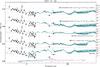 |
Fig. 2 Transmission spectra for the warm Saturn HAT-P-12b, along with the observational data taken from Sing et al. (2015a). For clarity, a vertical offset has been applied to the various models. The cloud species considered here are Na2S and KCl only. From top to bottom, the following cases are plotted: a) homogeneous clouds, with a maximum cloud mass fraction of Xmax = 3 × 10⁻⁴·ZPl per species and a single cloud particle size of 0.08 μm. Iron clouds have been neglected; b) like a), but including iron clouds; c) self-consistent clouds using the Ackerman & Marley (2001) model with fsed = 1; d) like c), but using fsed = 0.01; e) clear, fiducial atmospheric model. The colored bars at the bottom of the plot show the spectral range of the various JWST instrument modes. The dotted horizontal lines denote the pressure levels being probed by the transit spectra with the pressure values indicated on the right of the plot. |
First, an increase (or decrease) of the enrichment will result in an increased (or decreased) total opacity within the atmosphere. This is because the main carriers of the atmospheric opacities are the metals, rather than H2 and He. The effect of scaling the planetary enrichment on the atmospheric temperature structure and emission spectra has been studied in Mollière et al. (2015), and we only provide a brief outline here: a higher enrichment moves the photosphere position to smaller pressures, leading to less pressure broadening of lines and a decreased strength of the CIA opacity, because the strength of both these opacity sources scales linearly with pressure. Hence the opacity in the atmospheric windows decreases. This exposes deeper, hotter layers in the windows and leads to a larger contrast between emission minima and maxima in spectra. This effect, neglecting metallicity-dependent chemistry, is (inversely) degenerate with varying the planetary surface gravity as it holds that dτν = (κν/g)dP, where τν is the optical depth, κν the opacity, g the surface gravity and P the pressure.
Second, atmospheric transmission spectra are affected by scaling the metallicity in two ways: increasing the metallicity and therefore the total opacity will result in an increased transit radius, while a significant increase in metallicity and the resulting increase of the atmospheric mean molecular weight will weaken the signal amplitude between maxima and minima in the transmission spectrum, because R(λ) ∝ [kBT/ (μg)] ·log (κν) (Lecavelier des Etangs et al. 2008), where R(λ) is the planetary transit radius, kB the Boltzmann constant, T the atmospheric temperature, μ the atmospheric mean molecular weight and g the planetary surface gravity.
Finally, an increased enrichment will affect the atmospheric abundances because of the metallicity-dependent chemistry: the CO2 abundance, for example, is a strong function of metallicity (see, e.g. Moses et al. 2013, and references therein).
5.2. Clouds
The various cloud models investigated in this study are summarized in Sect. 4.2. Here we concentrate on the spectral characteristics of some of these cloud models. In Fig. 2 we show transmission spectra resulting from self-consistent atmospheric structure calculations of the planet HAT-P-12b, together with the observational data of the HST and Spitzer telescope (Sing et al. 2015a). We look at the cases including only Na2S and KCl clouds here. For these calculations, a planet-wide averaged insolation was assumed, because it was found that 3D GCM calculations lead to similar transmission spectra as the planet-wide averaged insolation 1D modes (but exceptions may exist; for more details see Fortney et al. 2010). Effects of patchy clouds, which may mimic the signal of high-mean-molecular-weight atmospheres (Line & Parmentier 2016), cannot be reproduced with this approach.
The model spectra plotted in Fig. 2 include the smaller and larger cloud particle (fsed = 0.01 and 1, respectively) self-consistent clouds following the Ackerman & Marley (2001) cloud model, as well as the parametrized homogeneous clouds with small particles of size 0.08 μm. Models are shown with and without the consideration of iron clouds. Finally, our fiducial, cloud-free model is shown as well. Note that we also draw horizontal lines in the plot that indicate the pressure being probed by the various models, corresponding to the (wavelength-dependent) effective radius. The optimal y-offset value of the spectra with respect to the data was found by χ2 minimization.
Before investigating the different cloudy models, we note that the clear atmosphere (Model (e) in Fig. 2) obviously represents a bad fit to the data: a simultaneous fit of the Rayleigh-like signature of the optical and NIR HST data and the Spitzer photometry at IR wavelengths is not possible. Note that the HST STIS and Spitzer data are both crucial for this claim of “cloudiness” because the measurement of a Rayleigh signal in the optical alone is not sufficient as it could be simply caused by H2 and He. Only a spectral slope less negative than −4 in the optical may allow us to infer the presence of large particle (a ≳ λ/ 2π) clouds from the spectrum alone, but this requires an accurate estimate of the atmospheric scale height (also see Heng 2016).
Studying the cloudy results in Fig. 2 one sees that only the parametrized homogeneous clouds with a particle size of 0.08 μm (model (a) in Fig. 2) are able to produce Rayleigh scattering ranging from the optical (~0.4 μm) to the NIR as probed by the HST data. Further, this is only possible if iron clouds are neglected: Due to the high absorption cross-section of iron in the optical the Fe clouds clearly decrease the spectral slope such that it is less strong than expected for pure Rayleigh scattering (see Model (b) in Fig. 2).
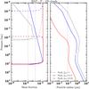 |
Fig. 3 Left panel: the solid lines denote the Na2S cloud-mass fractions as a function of pressure for the fsed = 0.01, 0.3, and 1 models, shown in red, blue, and gray, respectively. The dashed lines denote the mass fractions derived from equilibrium chemistry, that is, in the absence of mixing and settling. For a comparison, the four vertical lines denote the three different Xmax values used in the homogeneous cloud models. Right panel: mean cloud particle radii derived for the fsed = 0.01, 0.3, and 1 cloud models. Again for comparison, the vertical dotted line denotes the particle size a = 0.08μm adopted for the homogeneous cloud models. |
The results for the Ackerman & Marley (2001) clouds are shown in the models (c) and (d) in Fig. 2 for fsed = 1 and 0.01, respectively. Model (c) produces a flat slope in the optical and NIR and seems to mute the molecular features too strongly when compared to the data. For the self-consistent cloud with a small fsed = 0.01 value (model d) we find that the slope in the optical is already relatively steep, approaching a Rayleigh scattering slope. However, although the average particle size is well below 0.08 μm, the slope is less steep than in the mono-disperse particle model (a) because the largest particles within the distribution dominate the opacity (Wakeford & Sing 2015). We thus do not find a good fit for HAT-P-12b when using the Ackerman & Marley (2001) model. The broad absorption feature starting at 30 μm in the transmission spectrum of model (d) is the Na2S resonance feature.
We show the mean particle size obtained for the fsed = 0.01, 0.3, and 1 models in the right panel of Fig. 3, along with the cloud mass fractions in the left panel. Only Na2S condensed for the models presented here, because the atmosphere was too hot for KCl condensation to occur.
Note that the cloud mass fraction derived from our cloud model implementation starts already one layer below the layer where equilibrium chemistry first predicts condensation. This is due to the fact that the cloud source term in our implementation of the Ackerman & Marley (2001) model is proportional to d , where Xequ is the mass fraction of the condensate species derived from equilibrium chemistry. This derivative, evaluated between the two layers, leaves a non-zero cloud mass fraction at the lower layer when solved on a high-resolution grid between the layers and then interpolated back to the coarse resolution. The advantage of our implementation is that no knowledge of the saturation pressures of given condensates is required, and that one can simply use the output abundances of a Gibbs minimizer (see Appendix A.3 for more information). The true location of first condensation is located somewhere between the two layers. Due to the good agreement when comparing this to the example cases given in Ackerman & Marley (2001) we decided to keep the current treatment1.
Due to the large size of the cloud particles shown for the fsed = 1 model in Fig. 3, cloud resonance features in the MIR are hard to see in Fig. 2 (model c): Only small enough grains exhibit resonance features, while increasingly larger grains have flatter, more grayish opacities. Consequently, the Na2S feature at 30 μm can be seen more prominently for model (d), as this model results in smaller particle sizes.
To summarize, within our work, the Ackerman & Marley (2001) results correspond to clouds with broader particle size distributions which tend to produce transmission spectra that are either flat or less strongly sloped than expected from small particle Rayleigh scattering. For the smallest fsed values, we succeed in acquiring relatively steep scattering slopes, but at the same time the clouds are relatively optically thick, muting the molecular features more strongly. We point out that this does not mean that the (Ackerman & Marley 2001) model is not useful for fitting cloudy planetary spectra, but it is potentially more useful for transmission spectra that show a flat and gray cloud signature in the transmission spectrum, as is seen for GJ 1214b (see Morley et al. 2015, and our results for GJ 1214b using cloud model 4 in Sect. 6.1.)
Finally, some of the spectra we show in Fig. 2 may fit the transmission results relatively well. We want to remind the reader that we used the same cloud setups for all candidate planets presented in this paper, without trying to find the true best fit parameters according to our model. Therefore, a dedicated study for the individual planets may result in even better estimates of the atmospheric parameters. Furthermore, it is not correct to assume that the homogeneous clouds used for model (a) represent a good description of the cloud mass fraction and particle sizes throughout the whole atmosphere. As can be read off in Fig. 2, the maximum pressure being sensed by transmission in model (a) is approximately 10 mbar. Therefore, an equally good fit may be obtained using a cloud model that truncates the cloud at P> 10 mbar and sets the cloud density to zero at larger pressures. This may leave the transmission spectrum unchanged but will strongly affect the planet’s emission spectrum: as mentioned previously, it is well known that the emission spectra probe higher pressures than transmission spectra. This is due to the different trajectories of the light rays probing the atmosphere vertically in emission vs. the grazing geometry of light rays during transmission spectra. The vertical vs. the grazing optical depth at the photosphere of the planet may be different by a factor  (see Fortney 2005), which easily reaches a factor of 100 or larger. For instance, the retrieval analysis of HD 189733b requires clouds to fit the transmission spectrum, while the emission spectrum is fit well with a clear atmosphere (Barstow et al. 2014, a similar result could be obtained when considering a clear dayside and cloudy terminator regions, however).
Due to the assumption of homogeneous clouds, we obtain a Bond albedo of 17% for model (a) in Fig. 2. Model (b), which has the same Xmax value as model (a), only has an albedo of 5%, because the iron cloud particles absorb light effectively. For the self-consistent clouds, we obtain 10% for Model (c) and 8% for Models (d). The clear model (e) has an albedo of 3%. If clouds were truncated below the pressures probed by transmission, the albedos for the models would be lower.
In conclusion, it may well be the case, therefore, that the transmission spectrum of a planet is fit well by a cloudy atmosphere, while the planet’s emission spectrum is described well by the corresponding clear atmosphere. For HAT- P-12b, this assessment is impossible because the Spitzer eclipse photometry for the dayside emission by Todorov et al. (2013) only gives upper limits at 3.6 and 4.5 μm. These limits are consistent with all the model calculations we carried out for this planet for a planet-wide averaged insolation. The dayside averaged insolation case is excluded because all models have larger fluxes than allowed by the upper limits.
5.3. C/O
The importance of the C/O ratio for atmospheric chemistry and the effects arising from varying this parameter have been described in Seager et al. (2005), Kopparapu et al. (2012), Madhusudhan (2012), Moses et al. (2013), for example. Additionally, the dependence of properties of planetary atmospheres upon variation of the C/O ratio has been extensively and systematically studied in our previous study, Mollière et al. (2015), such that we only give a short summary here.
In Fig. 4, we show the emission spectra calculated for the warm Jupiter WASP-10b (Tequ = 972 K) and the hot Jupiter WASP-32b (Tequ = 1560 K), along with the Spitzer eclipse measurements by Kammer et al. (2015) and Garland et al. (2016), respectively. Note that both the synthetic spectra and data of WASP-32b have been multiplied by an offset factor of three in order to minimize the overlap between the spectra of WASP-10b and WASP-32b. We plot the spectra resulting from a dayside averaged insolation for both planets.
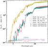 |
Fig. 4 Synthetic emission spectra of the planets WASP-32b and WASP-10b for the clear fiducial models with solar C/O ratios and for the cases with C/O ratios twice as large as solar. We also plot existing Spitzer photometry for the targets by Garland et al. (2016, WASP-32b) and Kammer et al. (2015, WASP-10b). A dayside-averaged insolation was assumed for both planets. For clarity, both the synthetic spectra and data of WASP-32b have been multiplied by an offset factor of three. |
For the hotter planet, WASP-32b, the spectra exhibit a clear dichotomy, with the solar C/O spectrum (C/O⊙ ~ 0.56) dominated by water absorption and the spectrum with twice the solar C/O value (1.12) dominated by methane absorption.
For the cooler planet, WASP-10b, the spectrum of the solar C/O case shows both water and methane absorption (see the telltale methane feature at 3.3 μm), while the C/O = 1.12 case shows methane absorption but no water absorption. The reason that lower-temperature atmospheres can show both water and methane absorption at the same time, regardless of the C/O ratio, can be understood by considering the net chemical equation CH4 + H2O ⇌ CO + 3H2, where the left-pointing direction is favored for low temperatures (≲1000 K) and high pressures (see, e.g., Lodders 2010). Note that depending on the vigor of vertical mixing, the transition temperature, below which the left-pointing direction is favored in the atmospheres of planets, may be as low as 500 K due to chemical quenching (Zahnle & Marley 2014). We do not model such non-equilibrium chemistry effects in our calculations. However, the importance of non-equilibrium chemistry strongly depends on the values of the mixing strength, which is related to the planetary surface gravity. Both planets shown here have relatively high surface gravities, which tends to decrease the mixing strength (Zahnle & Marley 2014) and shifts the location of the photosphere to higher pressures where the left-pointing direction of the above reaction equation is favored even more.
5.4. TiO/VO opacities
In the cases where equilibrium chemistry allows for TiO and VO to exist in the gas phase, and for the calculations for which we specifically include TiO and VO opacities, we find that the converged atmospheric solutions exhibit inversions. For cases where the atmospheres are cool enough such that Ti and V have condensed out of the gas phase, we find that the results are identical to our clear, fiducial calculations, which do not include TiO/VO opacities.
Atmospheres with TiO and VO inversions show emission spectra that are more isothermal than the corresponding fiducial cases, that is, the SED more closely resembles a blackbody, because the inversion decreases the overall temperature variation in the photospheric layers of the atmospheres. We stress that this does not mean that the atmospheres attain a globally more isothermal state; we still find strong inversions if the insolation and the TiO/VO abundances are high enough. The decreasing temperature variability merely holds for the photospheric region, not for the whole atmosphere: inversions form if the opacity of the atmosphere in the visual wavelengths is larger than in the IR wavelengths. When entering the atmosphere from the top, the optical depth for the stellar light reaches unity before the location of the planetary photosphere is reached. Therefore the higher atmospheric layers, in which a non-negligible amount of the stellar light is absorbed, need to heat up significantly in order to reach radiative equilibrium (i.e. absorbed energy equals radiated energy). These layers will cause the formation of emission features. On the other hand, the photosphere represents the region where the planet’s atmosphere radiates most of its flux to space, because here the IR optical depth reaches unity. This region is below the inversion region. Below the photosphere, the atmospheric temperature will increase monotonously. Consequently, the photosphere is bracketed by a region where the temperature decreases as one approaches the photosphere coming from the inversion above, and a region where the temperature increases again when moving on to larger pressures. Hence, the total temperate variation across the photospheric region, which is a region in which the atmospheric temperature gradient transitions from being negative to being positive, is small. Therefore the spectral energy distribution escaping from this region is closer to an isothermal blackbody than in an atmosphere without an inversion.
In transmission, these atmospheres exhibit TiO/VO resonance features in the optical and NIR, which are well known from theoretical calculations of atmospheric spectra (see, e.g. Fortney et al. 2008, 2010) but have not yet been conclusively detected in observations.
If we include TiO/VO opacities, all atmospheres with equilibrium temperatures higher than 1500 K show inversions in their atmospheres for the dayside averaged insolation calculations. In planet-wide averaged insolation calculations these planets showed inversions as well, but the planets with equilibrium temperatures below 1750 K had inversions that were relatively high in the atmospheres, such that either none or only weak emission features were seen. The transmission signatures of TiO/VO were seen in all cases that exhibited an inversion.
Instrument parameter values used for the synthetic JWST observations.
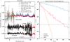 |
Fig. 5 Left panel: synthetic transit spectra, observations, and synthetic observations for the planet GJ 1214b. The orange points denote the observational data by Kreidberg et al. (2014), while brown points denote the observational data by Bean et al. (2010), Désert et al. (2011), Bean et al. (2011), Berta et al. (2012), Fraine et al. (2013). Synthetic spectra for the cloudy fsed = 0.3 model (Model 3 in Table 2) are shown as red or purple solid lines for the case including Na2S+KCl clouds or KCl clouds only. The clear model is shown as a teal line. A straight line model is shown as a thick gray solid line. The black dots show the synthetic observations derived for one (top) and ten (bottom) transits, re-binned to a resolution of 50. Vertical offsets have been applied for the sake of clarity. Right panel: p values of the Kolmogorov-Smirnov test for the residuals between the synthetic observation of the Na2S+KCl cloud model and the straight line model fitted to these observations. The p value is shown as a function of Ntransit for the three different instruments of Table 3. For every (instrument, Ntransit) setup, a new straight line model is fitted to the observations. The black dashed line denotes our threshold value of 10-3. |
6. Simulated observations
In this section we show the characteristics of the simulated observations carried out for all targets defined in Table 1. Similar to Sect. 5, we concentrate on a few, exemplary objects. Here we investigate how the simulated observations appear as a function of the number of transits/eclipses, and which wavelength ranges have the most diagnostic power for characterizing the planets.
The instrument parameters adopted to describe the performance of JWST are listed in Table 3. The values for the full well capacity and readout noise of the NIRSpec instrument were taken from Ferruit et al. (2014), and we adopted the same full well capacity for NIRISS, due to the similarity of the detectors. The noise floor for NIRSpec is expected to be below 100 ppm (Ferruit et al. 2014), and we adopt a value of 75 ppm here. Following Rocchetto et al. (2016) one may assume a noise floor value of 20 ppm for NIRISS. Further, we set the MIRI noise floor value to 40 ppm, because the values adopted in the existing literature range from 30 to 50 (see Beichman et al. 2014; Greene et al. 2016, respectively). The remaining instrument characteristics for MIRI were taken from (Ressler et al. 2015).
We publish synthetic observations corresponding to a single transit or eclipse measurement for every planet and every instrument. We note that for every instrument, a separate observation needs to be carried out. The data is given at the instruments’ intrinsic resolutions. In regions where the wavelength binning of petitCODE was coarser than the intrinsic resolution, we rebinned the spectra of petitCODE to this higher resolution. Lower resolution data may be obtained by rebinning the observations and propagating the errors during the process. We also publish the model spectra without observational noise along with the single observation errors, such that multiple transit/eclipse observations can be obtained by sampling the noiseless spectra using errors normalized with  .
.
6.1. Transmission spectroscopy
In this section we chose two different kinds of planets to show examples of our synthetic observations: super-Earth planets with flat transmission spectra, as well as hot Jupiters with steep Rayleigh signals. The target chosen here for the super-Earths is GJ 1214b, while for the hot Jupiters we investigate TrES-4b.
6.1.1. The case of extremely cloudy super-Earths: GJ 1214b
The observational data for GJ 1214b, as well as synthetic spectra and observations, are shown in the left panel of Fig. 5. For clarity, the synthetic observations have been re-binned to a resolution of 50. Note that the noise of the measurements increases with wavelength as less light is coming from the star at longer wavelengths. In addition to the cloudy fsed = 0.3 model (Model 3 in Table 2) shown in the plot, we also show a clear atmosphere for comparison. For this planet, cloud models 3 and 4 converged with the cloud feedback included. We therefore present self-consistent calculations for cloud model 3 for GJ 1214b.
It is evident that the clear spectrum is inconsistent with the HST data by Kreidberg et al. (2014), whereas cloudy models provide a better fit. The need for clouds has been studied in detail in Morley et al. (2013), Kreidberg et al. (2014), Morley et al. (2015), where Morley et al. (2013, 2015) found that high atmospheric enrichments are necessary to fit the data. They also put forward the possibility that the flat transmission spectrum of GJ 1214b could be caused by hydrocarbon hazes, and suggested pathways of how to distinguish between mineral clouds and hydrocarbon hazes using emission spectroscopy or by analyzing the reflected light from these planets.
Our cloudy spectrum is mostly flat from the optical to the NIR, but some molecular features can be made out clearly, especially in the MIR region, including the methane features at 2.3, 3.2, and 7.5 μm and the CO2 features at 2.7, 4.3, and 15 μm. The CO2 feature at 15 μm is not within the spectral range of the MIRI LRS instrument. Due to the high metallicity, CO2 is the most spectrally active carbon- and oxygen-bearing molecule and more abundant than CH4, CO, or H2O at the pressures being probed by the transmission spectrum. For a cloudy, highly enriched atmosphere, as presented here, we therefore predict the existence of CO2 and CH4 features in the otherwise flat transmission spectrum.
Because GJ 1214b is the coolest planet considered in our sample, we only include KCl and Na2S clouds in its atmosphere (see Sect. 4.2). However, even Na2S clouds may form too deeply in this atmosphere for them to be mixed up into the region probed in transmission Morley et al. (2013), Charnay et al. (2015a). Both approaches, excluding Na2S or including it, have been studied in the literature (Morley et al. 2013, 2015; Charnay et al. 2015b). We thus also show a comparison to a model solely including KCl clouds in Fig. 5. One sees that as the cloud opacity decreases, the molecular features can be seen more clearly.
The highest quality spectrum currently available for GJ 1214b is consistent with a straight line (Kreidberg et al. 2014). We therefore want to assess how well JWST observations could distinguish our high metallicity cloudy model from a flat featureless spectrum, as a function of the number of transits observed. As an example, we show a comparison model (a straight line spectrum) as a gray line in Fig. 5. The transit radius of the straight line model was chosen by fitting a synthetic single transit observation of the KCl+Na2S cloud model in all instruments with a straight line by means of χ2 minimization.
First we tested which instrument, that is, which wavelength range, is best suited for the task and how many transits are needed to conclusively rule out the straight line case. In order to avoid ruling out a straight line scenario because of an offset of the global (fitted for all three instruments) straight line model to a single instrument spectrum, we fitted straight line models to the synthetic observation within each instrument separately. For this, we generated synthetic observations Tλ (instrument,Ntransit), where the Tλ (instrument) denotes the observed wavelength-dependent transmission using one of the instruments listed in Table 3, and Ntransit is the number of transits accumulated to obtain the observation. For every (instrument, Ntransit) pair, we then fitted a straight line to the observations and calculated the residuals of the straight line to the cloudy observation, taking into account the appropriate errors when stacking Ntransit transits in the instrument of interest. The residuals were then compared to a Gaussian normal distribution using a Kolmogorov-Smirnov test2. To rule out the straight line model, given our observation of the cloudy model, we adopted a conservative threshold p value of 10-3. This means that the probability of observing a straight line model and finding the above distribution of residuals, or one that is even less consistent with a normal distribution, is 10-3. Alternatively to fitting a straight line model to the synthetic observations, it is also possible to adopt an arbitrary offset between the model and the observations and then shift the distribution of residuals between the straight line model and the cloudy model such that is has a mean value of zero. For this case we obtained identical results.
We show the resulting p values as a function of Ntransit in the right panel of Fig. 5 for the three different instruments. To minimize the Monte Carlo noise resulting from the generation of the synthetic observations, we took the median p value of 100 realizations for every (instrument, Ntransit) point. We find that NIRISS would not be able to rule out a straight line spectrum even if 50 spectra were stacked. This is due to the fact that the cloudy model is relatively flat in this wavelength region. With NIRSpec, on the other hand, the distinction may be possible by stacking 16 observations. For MIRI, a refutal of the straight line model is possible after ~40 transits. Thus, using our conservative p value threshold, it seems quite hard to refute the straight line case, although the NIRSpec observations look different from a straight line when inspected by eye already after less than ten transits in Fig. 5. Therefore, if one carries out the same test once more, but compares the observations with the cloudy model itself, one finds p values with a median of 1/2, independent of the number of transits. Hence, one may say that a cloudy model is more likely to describe the data than the straight line model, already after less than ~10 transits, if one uses the NIRSpec band and carries out a retrieval analysis. Note, however, that the p value is subject to statistical noise due to the limited number of spectral points.
The reason for the Kolmogorov-Smirnov test to require a relatively large number of transits for the distinguishability analysis presented here is that the triangularly shaped molecular features will lead to relatively symmetric residual distributions when compared to the straight line model. In this sense, it becomes harder for the Kolmogorov-Smirnov test to distinguish between the resulting residual distribution and a Gauss distribution, because this test is insensitive to the wavelength correlation of the residuals. For a conclusive statement, rather than an upper limit, regarding the number of transits needed for constraining GJ 1214b’s atmosphere, one therefore needs more sophisticated statistical tools, such as retrieval analyses. However, the Kolmogorov-Smirnov test may still be used to assess which instrument, and thus wavelength range, may be best suited for distinguishing the cloud GJ 1214b observation from a straight line and our analysis indicates that NIRSpec will be best suited for this task, followed by MIRI. NIRISS was found to be the least well suited.
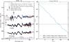 |
Fig. 6 Left panel: synthetic transit spectra, observations, and synthetic observations for the planet TrES-4b. Black crosses denote the ground-based observational data by Chan et al. (2011), Sozzetti et al. (2015), Turner et al. (2016). Black squares denote the HST WFC3 data by Ranjan et al. (2014). Synthetic spectra for the homogeneously cloudy models with Xmax = 3 × 10⁻⁴ZPl are shown as teal and red solid lines for the DHS and Mie opacity, respectively. The dashed box at ~10 μm highlights the silicates features due to Mg2SiO4 resonances.The teal and red dots show the corresponding synthetic observations derived for one and ten transits, re-binned to a resolution of 50. Vertical offsets have been applied for the sake of clarity. Right panel: p values of the Kolmogorov-Smirnov test of the residuals between the synthetic observation of the TrES-4b DHS model and the Mie model (solid teal line). The p value is shown as a function of Ntransit for data taken with MIRI LRS considering only the wavelength range of the silicate feature (9–13 μm) and correcting for global model offsets. The dashed teal line shows the p value obtained when analyzing the residuals of the DHS model to its own observation. The black dashed line denotes our threshold value of 10-3. |
Finally, we find that our KCl+Na2S cloud model presented for GJ 1214b in the left panel of Fig. 5 results in a p value of 0.45 if compared to the existing observational data. It is therefore consistent with these data.
6.1.2. TrES-4b
In the left panel of Fig. 6, we show the simulated transmission observations of TrES-4b. TrES-4b is a strongly inflated (1.7 R♃) hot Jupiter that circles its F-type host star (T∗ = 6200 K) once every 3.6 days (Chan et al. 2011). The dayside emission of this planet seems to be consistent with a temperature inversion (Knutson et al. 2009) and the dayside for this planet may therefore be too hot to have a significant silicate cloud coverage. However, the limbs may be much cooler than the bulk dayside, allowing for these clouds to exist (see, e.g. Wakeford et al. 2017). To account for this effect, we model the transmission spectra for the planets assuming a global redistribution of the stellar irradiation energy (also see Sect. 5.2). The theoretical global equilibrium temperature of this planet is 1795 K. It is therefore within the temperature range where mineral clouds such as Mg2SiO4 and MgAl2O4 can be expected.
We look now to synthetic observations for the cloud models 6 and 9 in Table 2, that is, homogeneously distributed clouds of small particles assuming either irregular (DHS) or spherically homogeneous (Mie) particles. For comparison we also show the clear model for this planet.
The feature at 10 μm in the cloudy models, which is highlighted by the dashed-line box in Fig. 6, arises from resonances of the crystalline Mg2SiO4 particles. The differences in the location and relative strength of the Mg2SiO4 resonance peaks, arising from the different particle shapes (irregular vs. spherically-homogeneous), are evident.
By carrying out a Kolmogorov-Smirnov analysis of the residuals between the clear model and the synthetic DHS cloud model observations, we find that a single transit in MIRI will be enough to discriminate between the clear and cloudy model. This implies that a single transit is sufficient for finding evidence for silicate cloud particles in such an atmosphere. Before carrying out the Kolmogorov-Smirnov analysis we corrected the offset between the two models in the MIR part shortward of 9 μm, which is fully determined by molecular features. This was done in order to prevent a model discrimination based purely on global model offsets.
While the existence of an extinction feature at 10 μm, spanning the wavelength range from ~8 to ~12 μm, would hint at the presence of silicate absorbers in the planet’s atmosphere, a single transit will not be enough to discriminate between all possible silicate absorbers: the resolution needed to resolve individual crystalline dust features is in the range of 50. Thus the number of stacked transits needs to guarantee a high enough S/N for a single point at this resolution. Juhász et al. (2009) have shown that for protoplanetary disks, the S/N required to characterize the silicate dust properties (crystallinity and size) well is between 10 and 100 per spectral point. In the example shown here we only consider crystalline Mg2SiO4 for the silicates. But also different silicates, such as MgSiO3, iron-enriched olivines and pyroxenes, or species such as SiO2, FeSiO3 and Fe2SiO4 are possible (see Wakeford & Sing 2015). Another complication arises from the wavelength-dependent shape and position of the absorption features for particles larger than ~1 μm, but note that a strong Rayleigh signal observed in the optical and NIR transmission spectrum would suggest particles that are smaller than 0.1 μm. Unfortunately, the currently available ground-based data for this planet exhibit a large spread such that conclusive statements regarding the optical and NIR part of the planet’s spectrum appear difficult.
In summary, this means that a single transit is not enough to fully characterize silicate dust based on the 10 μm feature in transmission spectra. However, if the need for small particle clouds is evident from the transmission spectrum, due to a strong Rayleigh signal in the optical and NIR, then the observation of a 10 μm feature presents strong evidence for the presence of silicate grains in the atmospheres, while the lack of such a feature means that the strong Rayleigh slope in the optical and NIR cannot be caused by silicates. In that sense JWST will shed light on the nature of small grain clouds by allowing us to find whether silicates are responsible or not, potentially using a single transit observation with MIRI.
In our idealized example shown here, where the only considered silicate species are crystalline Mg2SiO4 particles of either irregular or spherically-homogeneous shape, we can now asses how many transits would be needed to conclusively distinguish between both models. Similar to the Kolmogorov-Smirnov test carried out before for the clear and cloudy model, one can analyze the residuals of the Mie cloud model with respect to the observations of the DHS cloud model. The results are shown in the right panel of Fig. 6. Again, because the silicate features only occur in the MIRI wavelength regime, we concentrate on this instrument only for the analysis and only on the silicate feature, considering a wavelength range from 9 to 13 μm. In order to analyze only the difference in the cloud features we again corrected the cloud models for the offset that can be seen in the MIRI wavelength regime, outside of the silicate feature.
We find that the Mie cloud model is inconsistent with DHS observations if ~13–14 transits are stacked for this planet. Because we only considered two possible cloud models here, and not the full parameter space, the number of transits needed to characterize the state of the clouds may likely be higher, however. Again, looking at the ten transit observations in Fig. 6, a discrimination between the two cases seems to already be possible at a smaller number or transits. Therefore, similar to the analysis carried out for GJ 1214b in Sect. 6.1.1, we expect that statistical tools more powerful than the ones used here should be able to retrieve this difference for a smaller number of transits.
The two cloudy models shown in Fig. 6 are consistent with the observational HST and Spitzer data, resulting in p values of 0.20 an.d 0.25 for the DHS and Mie cases, respectively.
6.2. Emission spectroscopy
In this section we will investigate simulated eclipse observations of our targets using JWST. We concentrate on a very interesting class of emission targets, namely the hottest hot Jupiters in our target selection: WASP-33b, Kepler-13Ab, and WASP-18b. Along with their high equilibrium temperatures, these planets share an additional similarity: their spectra can all be approximated well by blackbody emission, yet all of them are best fit by inversions in their atmospheres, see Haynes et al. (2015), Shporer et al. (2014) and Nymeyer et al. (2011) for WASP-33b, Kepler-13Ab, and WASP-18b respectively. Further examples for such planets in the literature are TrES-3b (Croll et al. 2010) and WASP-24b (Smith et al. 2012).
The case of WASP-18b is especially intriguing. Based on the orbital and stellar parameters, the planet’s theoretical equilibrium temperature (i.e., assuming a planet-wide average of the insolation) is Tequ = 2410 K. If one assumes a dayside averaging of the insolation flux then the dayside effective temperature Tirr would be 2870 K. Yet, the measured dayside emission flux of this planet is consistent with brightness temperatures between 3100 and 3300 K, and the spectrum can be fit reasonably well by a blackbody at 3200 K (although an inversion fits better, see Nymeyer et al. 2011). Theoretically, the maximum flux that can be measured for an irradiated planet when observed during transit geometry, and when assuming blackbody emission, is equal to the flux emitted by a blackbody of temperature  , where T∗ is the stellar effective temperature, R∗ the stellar radius and a the planet’s semi-major axis. Note that the shape of the SED of such a planet would correspond to an even higher temperature, because the planet must emit all flux close to the substellar point and into the direction of the observer: if the planet truly had a global temperature of , it would violate energy conservation, emitting more flux than it receives from the star.
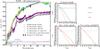 |
Fig. 7 Left panel: synthetic spectra and observational data of the emission spectrum of WASP-18b. A description of the different lines is shown in the legend. The observational data by Nymeyer et al. (2011) are shown as black errorbars. The “emission” lines, which can be made out in the blackbody FPl/F∗ spectrum, are absorption lines of the stellar spectrum. The colored circles show the corresponding Spitzer channels for the synthetic spectra. Right panel: p values of the Kolmogorov-Smirnov test of the residuals between the synthetic observation of the three WASP-18b models and the two respective remaining models. The p value is shown as a function of Ntransit for data taken with the three different instruments listed in Table 3. In order to avoid distinguishing between the models based on offsets, the residual distributions were shifted to have a mean value of 0. The black dashed line denotes our threshold value of 10-3. If an instrument is not shown in one of the three sub-panels then it has a p value lower than 10-12 already after one observation. |
For WASP-18b, Tmax = 3410 K, such that the planet’s corresponding blackbody temperature of 3200 K is still below this theoretical limit. Nonetheless, this suggests that a non-negligible fraction of the planetary flux must be emitted close to the location of the substellar point and thus into the direction of the observer during eclipse geometry. One can also see this by considering the insolation flux received by each circular planetary annulus at an angle θ away from the substellar point, which is 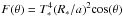 . If one neglects any energy redistribution due to winds, then the planetary surface at angle θ away from the substellar point has to re-emit exactly F(θ). Assuming blackbody emission, one finds that the flux measured during transit geometry is the same as if the planet had a global temperature of
  , which corresponds to 3080 K for WASP-18b. This is less than the stated blackbody temperature of 3200 K, suggesting that for this planet, energy redistribution may not only be limited, but fully absent.
The same situation seems to be the case for Kepler-13Ab, which is best fit by an inversion in its atmosphere, yet also reasonably well described by a blackbody at 2750 K (Shporer et al. 2014). For this planet, the theoretical upper limit on the observable effective temperature, as seen during eclipse geometry, is Tmax = 3085 K, the temperature derived for the case fully neglecting energy redistribution is Trad = 2790 K, the dayside averaged effective temperature is Tirr = 2590 K, if nightside emission is neglected, and the global equilibrium temperature would be Tequ = 2180 K. The measured effective temperature of the planet is closest to Trad, suggesting that wind redistribution of stellar insolation energy may be neglected for this planet as well. Interestingly, and quite paradoxically, Shporer et al. (2014) derive a geometric albedo of  for this planet, corresponding to a bond albedo of 0.5, if a matte, that is, perfectly Lambertian, scattering process is assumed. This albedo value arises from the fact that the optical eclipse depth for this planet shows an excess, which cannot be explained by 1D model calculations investigated in Shporer et al. (2014). The effective blackbody temperature derived from emission observations in the infrared (2750 K) is inconsistent with a bond albedo of 0.5, for which Tmax would be only 2590 K. We note, however, that the derivation of the geometric albedo in Shporer et al. (2014) assumed that the brightness temperature as well as the geometric albedo are constant within the three different bands used in their analysis, which is not necessarily the case. Further, the presence of scattering aerosols in the planet’s atmosphere in this high albedo case requires particles that are stable even at the high temperatures found for this planet, which is challenging. The measured excess of the optical eclipse depth may therefore be the emission feature of an unknown opacity source.
The planet WASP-33b is less extreme, because its theoretical dayside averaged effective temperature is Tirr = 3250 K, that is, still above the value derived when a blackbody is fitted to the emission observations (2950 K, see Haynes et al. 2015). Note that this planet is also fit better by an inversion than by a blackbody.
Given the fact that WASP-18b and Kepler-13Ab seem to have only limited, or no redistribution of the stellar insolation energy at all, we decided to calculate spectra for these planets fully neglecting the redistribution using Scenario (iii) described in Sect. 4.5.
We show the resulting spectra in the left panel of Fig. 7, together with the data by Nymeyer et al. (2011). No offset or scaling factor was applied to the synthetic spectra. As one can see, our fiducial case (no clouds, solar C/O ratio, and no TiO/VO opacities) is least capable to fit the data, being multiple sigmas away from all the measured points. For comparison, we also plot the fiducial case when assuming a dayside averaged insolation. In this case, the synthetic spectrum is even further away from the data.
Only three scenarios provide a good fit to the data; namely the case where we included TiO/VO opacities, which lead to an inversion, the case where we consider a C/O that is twice the solar value, leading to C/O = 1.12, and the case where we assume the planetary annuli to emit as isothermal blackbodies. It was crucial to neglect redistribution for these cases. The corresponding dayside-averaged cases resulted in fluxes that were too low. The “emission” lines, which can be made out in the blackbody FPl/F∗ spectrum, are absorption lines of the stellar spectrum.
We note that the Spitzer point at 4.5 μm does not seem to be fitted by the models. However, a good fit to data is not about the model perfectly describing every data point. In fact, if the error bars of a measurement are estimated accurately, then one expects that one third of all measured points are further than 1σ away from the prediction of the “correct” model. To assess the goodness of fit of the models to the data we will again make use of the Kolmogorov Smirnov test. Note that χ2 may be used to compare the various models against each other, but not to assess the overall goodness of fit of a given model: for a linear model, the expected value of a model correctly describing the data is χ2 = #dgf, where #dgf is the number of degrees of freedom, such that  . However, the spectral models we use here are non-linear, with the exact number of the degrees of freedom unknown. The expected χ2 value of a model consistent with the data can therefore not be calculated, and the use of the χ2 to assess the goodness of fit is not allowed (also see Andrae et al. 2010). The p value of the Kolmogorov Smirnov test applied on the residuals between the WASP-18b Spitzer measurements and the data, on the other hand, represents a valid method for assessing the goodness of fit. The p values for the TiO/VO, C/O = 2 × (C/O)⊙ and blackbody model are 0.38, 0.82 and 0.13, respectively. All models are therefore consistent with the data, with the best fit being provided by the C/O = 2 × (C/O)⊙ model.
For the high temperatures considered here, gaseous SiO may become important because the dayside of the planet is too hot to form any silicate clouds. We neglect the opacity of SiO, but this molecule is a strong UV absorber for λ< 0.3μm (see, e.g., Sharp & Burrows 2007) and may therefore lead to even stronger inversions. In future calculations, an inclusion of the SiO opacities for these hottest planets is therefore necessary.
The C/O = 1.12 case fits the data well because C/O ratios close to 1 may cause inversions, see Mollière et al. (2015). Such inversions form because for C/O ratios close to 1, oxygen and carbon are predominantly locked up in CO, decreasing the abundance of water if approached from C/O < 1, or that of methane if approached from C/O > 1. Because water and methane have large IR opacities, they are the atmosphere’s most effective coolant. Therefore, for C/O ~ 1, the cooling ability of the atmospheres is decreased, while the heating due to the alkali absorption of stellar light stays strong (we highlight that we include equilibrium ionization for sodium and potassium).
Given the fact that the blackbody emission case fits the data well, one can also understand why the inversion cases provide a good fit to the data: the inversion stops the monotonous decrease of temperature within the atmosphere, leading to smaller temperature variations across the photosphere. The photosphere therefore becomes more isothermal (also see Sect. 5.4).
Similar to the analyses carried out for the transiting planets, we now look into the number of transits needed to distinguish between the three models, which fit the observational data best. Applying an offset to the spectra for the emission spectra presented here would violate energy conservation, therefore we carry out the analysis without applying an offset at first. In this case the spectra of the three models can be distinguished from each other using only a single eclipse observation, in either of the three instruments considered here.
However, in order to assess how well the models may be distinguished because of differences in their spectral shape, we next applied an offset to the models before carrying out the Kolmogorov-Smirnov test. This was done by shifting the mean value of the residual distribution to zero. The corresponding plots are shown in the right panel of Fig. 7. Physically, such an offset may be motivated by a non-negligible redistribution of the stellar insolation, decreasing the planetary flux measured during an eclipse observation. We note that a simple offset as carried out here is only an approximation because the spectral shape may change under such conditions.
In general, the results follow our expectations: JWST is less capable of distinguishing between the TiO/VO and the blackbody case because the TiO/VO case does not have many features and is mostly simply offset in comparison to the blackbody model. This is especially true in the MIRI wavelength range, such that ten transits are not enough to distinguish between the two models at high confidence because we do not allow for the distinction between two models based simply on of an offset: this is why we applied the aforementioned shift of the residual distribution. The instrument best suited for distinguishing both models is NIRSpec, achieving this goal in just four transits.
JWST’s capability of distinguishing the CO = 1.12 and the blackbody case is much better, due to features visible in the spectrum of the CO = 1.12 case: The features at 3 μm, 6.5 to 8.5 μm and from 11 μm onward all stem from HCN absorption (not emission), whereas the feature at 4.5 μm is caused by CO absorption. These are typical absorbers expected for a hot, carbon-rich atmosphere. Because the NIRISS wavelength range is devoid of any molecular features, observations here will not help to distinguish between the models. The largest diagnostic power is provided by using NIRSpec observations (one eclipse measurement) while MIRI can discriminate between the models after three eclipse measurements.
The easiest case to distinguish is the case when comparing the C/O = 1.12 to the TiO/VO model because both these cases show molecular features. Again, NIRSpec is best at achieving this goal, using just a single transit, whereas MIRI and NIRISS need two and three transits, respectively. In conclusion, one can therefore say that if one of our self-consistent models was the true state of the atmosphere, then JWST could determine its state by taking between one and four transits in NIRSpec. Of course we do not prove that the three models here are the only possible ones, but our example illustrates the foreseen diagnostic power of JWST for such atmospheres.
7. Format and extent of the published atmospheric structures, synthetic spectra and observations
For all target planets listed in Table 1, we publish the self-consistent atmospheric structures listing the pressure, temperature, density, mean molecular weight, and specific heat cP for each atmospheric layer. We also publish the mass and number fractions of all chemical species as well as the mass fractions of all cloud species derived from the cloud models and the mean cloud particle sizes for every layer.
Further, we publish emission model spectra, reflected light spectra and transmission spectra from 110 nm to 250 μm. Additionally, we publish spectra restricted and rebinned to the JWST wavelength range and intrinsic resolution of the instruments listed in Table 3. For these rebinned spectra we publish single transit/eclipse errorbars, such that observations at any number of transits may be obtained by Gauss-sampling the noiseless spectra using errorbars scaled with  . Lower-resolution observations can be obtained by rebinning the observations and propagating the observational errors.
These data are published for all scenarios considered for the target planets, that is, varying the enrichment, C/O ratio, irradiation treatment, and cloud model, including TiO/VO opacities etc.
We publish all these data as described above in order to enable users to reproduce our calculations if desired and to be able to study the calculations as well as possible. Tests regarding the observational distinguishability via the Kolmogorov-Smirnov method as introduced in Sect. 6 are possible with the data as well as testing whether or not retrieval codes are able to constrain the atmosphere parameters as given in our published data.
8. Summary and conclusion
In this study we present a set of self-consistent atmospheric calculations for prime transiting exoplanet targets to be observed with JWST. We publish the resulting atmospheric structures, abundances and transmission and emission spectra. For the spectra, we additionally publish wavelength dependent uncertainties for JWST observations derived from radiometric modeling. By sampling the noiseless data using these errors, synthetic observations can be obtained.
The exoplanet targets have been chosen because they have a high expected S/N, cover the Tequ–log (g) space homogeneously, and include planet types ranging from super-Earths to hot Jupiters. This diverse set of targets may therefore allow the study of the full breadth of transiting exoplanets at high S/N.
Because the data currently available for these planets is often limited, both in its spectral coverage and S/N, it is crucial to explore different atmospheric scenarios in order to assess the width of possible observational results that may be seen once JWST becomes available. To this end, we explore a wide range of scenarios by varying the planets’ enrichment and composition (C/O ratio), and optionally include absorbers in the optical (TiO/VO) and put a large emphasis on studying the effects of different cloud properties. Furthermore, we apply different assumptions for the heat-redistribution; this we mimic by changing the irradiation, assuming either a planet-wide or dayside average of the irradiation. For some selected, very hot planets we also study the case of fully neglecting the redistribution of stellar irradiation.
Given the large uncertainties when trying to model clouds self-consistently, we study two cloud model setups, using either our implementation of the (Ackerman & Marley 2001) cloud model, for which we publish a new derivation, or by applying a parametrized cloud model. In the latter model, we set the cloud mass fractions equal to the condensate mass fraction obtained from equilibrium chemistry, but impose an upper boundary as a free parameter. Another free parameter is the particle size for the mono-disperse size distribution. This model therefore represents the case of vertically homogeneous clouds with mono-disperse particle distributions. Because cloud particles in planetary atmospheres are expected to be crystalline, rather than amorphous, we use optical constants for crystalline material whenever available. Additionally, all direct detections of crystalline silicate grains in different astrophysical contexts suggest that the grains should be irregularly shaped dust agglomerates, such that this is our standard assumption. The case of spherically-homogeneous cloud particles, with opacities derived from standard Mie theory, is studied as an optional case.
All calculations presented here are compared to observational data whenever available. For a selected subset of our targets, we study and compare different models that are consistent with the available data, and investigate how well JWST may be at distinguishing these models, and which instrument is best used for this task. The method we use for this subset study may be applied to any models within our grid. We summarize the main findings of this study below.
-
Super-Earths with thick cloud cover were studied byinvestigating our models for GJ 1214b. We findthat if we assume a heavy enrichment(1000 × solar) and a thick cloud deck then our models are consistent with current observational data. While the current data are consistent with a completely flat, featureless spectrum, we find that <10 transits with the NIRSpec instrument may be sufficient to unambiguously reveal CO2 and CH4 features in the atmosphere of this planet. For a more conclusive statement on the number of transits needed to characterize this planet, given our model, more sophisticated statistical tools, such as retrieval analyses are required. We plan to carry out such analyses as a next step.
-
Gas giants were studied by investigating our models calculated for HAT-P-12b and TrES-4b. In concordance with previous studies, we find that vertically homogeneous, small particle (<0.1 μm) clouds are best at producing strong Rayleigh scattering signatures, but only if iron-bearing cloud species are neglected. For TrES-4b, we expect a feature at 10 μm in the transmission spectrum if it harbors clouds that are made up from such small silicate particles. We find that one transit with MIRI may be sufficient to reveal the 10 μm feature, while less than ten transits may be enough to distinguish between irregularly shaped or spherically-homogeneous cloud particles, if the silicate species is known. Similarly, more sophisticated statistical tools will improve the analysis of the minimum number of transits required. A full characterization of silicate cloud particles (species, size distribution, vertical extent, particle shape, etc.) will likely require more transits.
-
Extremely hot transiting planets are often well fitted by isothermal emission when comparing to the data from eclipse measurements. We study the planet WASP-18b as an example and find that self-consistent models can explain the observations of this planet if energy redistribution by winds is fully neglected. The model setups which fit current observational data best are models featuring inversions either because of TiO/VO absorption or because of C/O number ratios close to 1. In this latter scenario, the main coolants (water or methane and HCN) are significantly depleted in favor of CO, such that inversions form. We find that a single eclipse observation with NIRSpec is enough to distinguish between these cases.
By investigating these three example cases, we show that JWST will be able to shed light on many intriguing puzzles of atmospheric studies that are difficult to solve using today’s observational facilities. Further, by publishing our atmospheric model calculations along with synthetic observational uncertainties for JWST we allow for the study of different possible scenarios and how well they can be observed and distinguished.
It has to be kept in mind that pitting given models against each other does not answer how conclusively we will be able to characterize a given atmosphere using JWST data. For such assertions, retrieval studies for the synthetic models would have to be carried out, and the results compared to the input model, as was done in Greene et al. (2016), but even then the conclusions depend on the input models. Nonetheless, studying the atmospheric models for the target planets as presented here enables us to evaluate the power of JWST at constraining the atmospheric state given various likely, self-consistent solutions for the investigated planets, which are consistent with the data available today.
Finally, because the full models are published, including temperature and abundance structures, retrieval models may be tested on our grid, allowing for the study of the retrievability of the expected JWST observations when considering self-consistent atmospheric models.
For the comparison study we adopted the same mixing length choice as in Ackerman & Marley (2001).
We used the kstest() function of the Scipy library for this task, see http://docs.scipy.org
Acknowledgments
P.M. thanks J.-L. Baudino, B. Bezard, C. Dullemond, E. Ford, H.-P. Gail, D. Homeier, C. Jäger, H.-G. Ludwig, C. Mordasini, V. Parmentier, P. Tremblin, and A. Wolfgang for useful discussions and helpful comments. P.O.L. acknowledges support from the LabEx P2IO, the French ANR contract 05-BLAN-NT09-573739.
References
- Ackerman, A. S., & Marley, M. S. 2001, ApJ, 556, 872 [NASA ADS] [CrossRef] [Google Scholar]
- Agúndez, M., Parmentier, V., Venot, O., Hersant, F., & Selsis, F. 2014, A&A, 564, A73 [NASA ADS] [CrossRef] [EDP Sciences] [Google Scholar]
- Ali-Dib, M., Mousis, O., Petit, J.-M., & Lunine, J. I. 2014, ApJ, 785, 125 [NASA ADS] [CrossRef] [Google Scholar]
- Alibert, Y., Carron, F., Fortier, A., et al. 2013, A&A, 558, A109 [NASA ADS] [CrossRef] [EDP Sciences] [Google Scholar]
- Andrae, R., Schulze-Hartung, T., & Melchior, P. 2010, ArXiv e-prints [arXiv:1012.3754] [Google Scholar]
- Asplund, M., Grevesse, N., Sauval, A. J., & Scott, P. 2009, ARA&A, 47, 481 [NASA ADS] [CrossRef] [Google Scholar]
- Barstow, J. K., & Irwin, P. G. J. 2016, MNRAS, 461, L92 [NASA ADS] [CrossRef] [Google Scholar]
- Barstow, J. K., Aigrain, S., Irwin, P. G. J., et al. 2014, ApJ, 786, 154 [NASA ADS] [CrossRef] [Google Scholar]
- Barstow, J. K., Aigrain, S., Irwin, P. G. J., Kendrew, S., & Fletcher, L. N. 2015, MNRAS, 448, 2546 [NASA ADS] [CrossRef] [Google Scholar]
- Barstow, J. K., Aigrain, S., Irwin, P. G. J., & Sing, D. K. 2017, ApJ, 834, 50 [Google Scholar]
- Baruteau, C., Bai, X., Mordasini, C., & Mollière, P. 2016, Space Sci. Rev., 205, 77 [NASA ADS] [CrossRef] [Google Scholar]
- Batalha, N., Kalirai, J., Lunine, J., Clampin, M., & Lindler, D. 2015, ArXiv e-prints [arXiv:1507.02655] [Google Scholar]
- Baudino, J.-L., Bézard, B., Boccaletti, A., et al. 2015, A&A, 582, A83 [NASA ADS] [CrossRef] [EDP Sciences] [Google Scholar]
- Bean, J. L., Miller-Ricci Kempton, E., & Homeier, D. 2010, Nature, 468, 669 [NASA ADS] [CrossRef] [PubMed] [Google Scholar]
- Bean, J. L., Désert, J.-M., Kabath, P., et al. 2011, ApJ, 743, 92 [NASA ADS] [CrossRef] [Google Scholar]
- Beichman, C., Benneke, B., Knutson, H., et al. 2014, PASP, 126, 1134 [NASA ADS] [CrossRef] [Google Scholar]
- Benneke, B. 2015, ApJ, submitted [arXiv:1504.07655] [Google Scholar]
- Berta, Z. K., Charbonneau, D., Désert, J.-M., et al. 2012, ApJ, 747, 35 [NASA ADS] [CrossRef] [Google Scholar]
- Biddle, L. I., Pearson, K. A., Crossfield, I. J. M., et al. 2014, MNRAS, 443, 1810 [NASA ADS] [CrossRef] [Google Scholar]
- Bouwman, J., Meeus, G., de Koter, A., et al. 2001, A&A, 375, 950 [NASA ADS] [CrossRef] [EDP Sciences] [Google Scholar]
- Burch, D. E., Gryvnak, D. A., Patty, R. R., & Bartky, C. E. 1969, J. Opt. Soc. Am., 59, 267 [NASA ADS] [CrossRef] [Google Scholar]
- Cáceres, C., Kabath, P., Hoyer, S., et al. 2014, A&A, 565, A7 [NASA ADS] [CrossRef] [EDP Sciences] [Google Scholar]
- Chan, Y. M., & Dalgarno, A. 1965, Proc. Phys. Soc., 85, 227 [Google Scholar]
- Chan, T., Ingemyr, M., Winn, J. N., et al. 2011, AJ, 141, 179 [NASA ADS] [CrossRef] [Google Scholar]
- Chandrasekhar, S. 1950, in Radiative transfer (Oxford University Press), 393 [Google Scholar]
- Charnay, B., Meadows, V., & Leconte, J. 2015a, ApJ, 813, 15 [NASA ADS] [CrossRef] [Google Scholar]
- Charnay, B., Meadows, V., Misra, A., Leconte, J., & Arney, G. 2015b, ApJ, 813, L1 [NASA ADS] [CrossRef] [Google Scholar]
- Cridland, A. J., Pudritz, R. E., & Alessi, M. 2016, MNRAS, 461, 3274 [Google Scholar]
- Croll, B., Jayawardhana, R., Fortney, J. J., Lafrenière, D., & Albert, L. 2010, ApJ, 718, 920 [NASA ADS] [CrossRef] [Google Scholar]
- Crossfield, I. J. M., Barman, T., Hansen, B. M. S., Tanaka, I., & Kodama, T. 2012, ApJ, 760, 140 [NASA ADS] [CrossRef] [Google Scholar]
- Crossfield, I. J. M., Barman, T., Hansen, B. M. S., & Howard, A. W. 2013, A&A, 559, A33 [NASA ADS] [CrossRef] [EDP Sciences] [Google Scholar]
- Cushing, M. C., Roellig, T. L., Marley, M. S., et al. 2006, ApJ, 648, 614 [NASA ADS] [CrossRef] [Google Scholar]
- Dalgarno, A., & Williams, D. A. 1962, ApJ, 136, 690 [NASA ADS] [CrossRef] [Google Scholar]
- de Mooij, E. J. W., Brogi, M., de Kok, R. J., et al. 2013, A&A, 550, A54 [NASA ADS] [CrossRef] [EDP Sciences] [Google Scholar]
- Deming, D., Seager, S., Winn, J., et al. 2009, PASP, 121, 952 [NASA ADS] [CrossRef] [Google Scholar]
- Deming, D., Fraine, J. D., Sada, P. V., et al. 2012, ApJ, 754, 106 [NASA ADS] [CrossRef] [Google Scholar]
- Deming, D., Knutson, H., Kammer, J., et al. 2015, ApJ, 805, 132 [NASA ADS] [CrossRef] [Google Scholar]
- Demory, B.-O., & Seager, S. 2011, ApJS, 197, 12 [NASA ADS] [CrossRef] [Google Scholar]
- Demory, B.-O., Torres, G., Neves, V., et al. 2013, ApJ, 768, 154 [NASA ADS] [CrossRef] [Google Scholar]
- Désert, J.-M., Bean, J., Miller-Ricci Kempton, E., et al. 2011, ApJ, 731, L40 [NASA ADS] [CrossRef] [Google Scholar]
- Doyon, R., Hutchings, J. B., Beaulieu, M., et al. 2012, SPIE Conf. Ser., 8442, 2 [Google Scholar]
- Dragomir, D., Benneke, B., Pearson, K. A., et al. 2015, ApJ, 814, 102 [NASA ADS] [CrossRef] [Google Scholar]
- Ehrenreich, D., Bonfils, X., Lovis, C., et al. 2014, A&A, 570, A89 [NASA ADS] [CrossRef] [EDP Sciences] [Google Scholar]
- Evans, T. M., Sing, D. K., Wakeford, H. R., et al. 2016, MNRAS, 822, L4 [Google Scholar]
- Fabian, D., Jäger, C., Henning, T., Dorschner, J., & Mutschke, H. 2000, A&A, 364, 282 [NASA ADS] [Google Scholar]
- Ferruit, P., Bagnasco, G., Barho, R., et al. 2012, SPIE Conf. Ser., 8442, 2 [Google Scholar]
- Ferruit, P., Birkmann, S., Böker, T., et al. 2014, in Space Telescopes and Instrumentation 2014: Optical, Infrared, and Millimeter Wave, Proc. SPIE, 9143, 91430A [Google Scholar]
- Fischer, P. D., Knutson, H. A., Sing, D. K., et al. 2016, ApJ, 827, 19 [CrossRef] [Google Scholar]
- Fortney, J. J. 2005, MNRAS, 364, 649 [NASA ADS] [CrossRef] [Google Scholar]
- Fortney, J. J., & Nettelmann, N. 2010, Space Sci.Rev., 152, 423 [NASA ADS] [CrossRef] [Google Scholar]
- Fortney, J. J., Lodders, K., Marley, M. S., & Freedman, R. S. 2008, ApJ, 678, 1419 [NASA ADS] [CrossRef] [Google Scholar]
- Fortney, J. J., Shabram, M., Showman, A. P., et al. 2010, ApJ, 709, 1396 [NASA ADS] [CrossRef] [Google Scholar]
- Foster, A. S., Harrington, J., Cubillos, P., et al. 2016, Amer. Astron. Soc. Meet. Abstracts, 227, 212.05 [Google Scholar]
- Fraine, J. D., Deming, D., Gillon, M., et al. 2013, ApJ, 765, 127 [NASA ADS] [CrossRef] [Google Scholar]
- Fukui, A., Kawashima, Y., Ikoma, M., et al. 2014, ApJ, 790, 108 [NASA ADS] [CrossRef] [Google Scholar]
- Gail, H.-P. 2001, A&A, 378, 192 [NASA ADS] [CrossRef] [EDP Sciences] [Google Scholar]
- Gail, H.-P. 2004, A&A, 413, 571 [NASA ADS] [CrossRef] [EDP Sciences] [Google Scholar]
- Garland, J., Harrington, J., Cubillos, P., et al. 2016, Am. Astron. Soc. Meet. Abstr., 227, 212.06 [Google Scholar]
- Gordon, S., & McBride, B. J. 1994, Computer Program for Calculation of Complex Chemical Equilibrium Compositions and Applications, Part 1: Analysis, National Aeronautics and Space Administration, Washington, D.C. 20546-0001 (USA: NASA) [Google Scholar]
- Greene, T. P., Line, M. R., Montero, C., et al. 2016, ApJ, 817, 17 [NASA ADS] [CrossRef] [Google Scholar]
- Grillmair, C. J., Burrows, A., Charbonneau, D., et al. 2008, Nature, 456, 767 [NASA ADS] [CrossRef] [PubMed] [Google Scholar]
- Gustafsson, B., Edvardsson, B., Eriksson, K., et al. 2008, A&A, 486, 951 [NASA ADS] [CrossRef] [EDP Sciences] [Google Scholar]
- Harker, D. E., & Desch, S. J. 2002, ApJ, 565, L109 [NASA ADS] [CrossRef] [Google Scholar]
- Hartmann, J.-M., Boulet, C., Brodbeck, C., et al. 2002, J. Quant. Spec. Radiat. Transf., 72, 117 [NASA ADS] [CrossRef] [Google Scholar]
- Harvey, A. H., Gallagher, J. S., & Levelt Sengers, J. M. H. 1998, J. Phys. Chem. Ref. Data, 27, 761 [NASA ADS] [CrossRef] [Google Scholar]
- Haynes, K., Mandell, A. M., Madhusudhan, N., Deming, D., & Knutson, H. 2015, ApJ, 806, 146 [NASA ADS] [CrossRef] [Google Scholar]
- Helling, C., Ackerman, A., Allard, F., et al. 2008, MNRAS, 391, 1854 [NASA ADS] [CrossRef] [Google Scholar]
- Helling, C., Woitke, P., Rimmer, P. B., et al. 2014, Life, 4, 142 [NASA ADS] [CrossRef] [Google Scholar]
- Heng, K. 2016, ApJ, 826, L16 [NASA ADS] [CrossRef] [Google Scholar]
- Henning, T., & Stognienko, R. 1996, A&A, 311, 291 [NASA ADS] [Google Scholar]
- Iyer, A. R., Swain, M. R., Zellem, R. T., et al. 2016, ApJ, 823, 109 [NASA ADS] [CrossRef] [Google Scholar]
- Jaeger, C., Molster, F. J., Dorschner, J., et al. 1998, A&A, 339, 904 [NASA ADS] [Google Scholar]
- Jin, S., Mordasini, C., Parmentier, V., et al. 2014, ApJ, 795, 65 [NASA ADS] [CrossRef] [Google Scholar]
- Jordán, A., Espinoza, N., Rabus, M., et al. 2013, ApJ, 778, 184 [NASA ADS] [CrossRef] [Google Scholar]
- Juhász, A., Henning, T., Bouwman, J., et al. 2009, ApJ, 695, 1024 [NASA ADS] [CrossRef] [Google Scholar]
- Juhász, A., Bouwman, J., Henning, T., et al. 2010, ApJ, 721, 431 [NASA ADS] [CrossRef] [Google Scholar]
- Kammer, J. A., Knutson, H. A., Line, M. R., et al. 2015, ApJ, 810, 118 [NASA ADS] [CrossRef] [Google Scholar]
- Kemper, F., Vriend, W. J., & Tielens, A. G. G. M. 2004, ApJ, 609, 826 [NASA ADS] [CrossRef] [Google Scholar]
- Kippenhahn, R., & Weigert, A. 1990, Stellar Structure and Evolution (Berlin, Heidelberg: Springer Verlag) [Google Scholar]
- Knutson, H. A., Charbonneau, D., Burrows, A., O’Donovan, F. T., & Mandushev, G. 2009, ApJ, 691, 866 [NASA ADS] [CrossRef] [Google Scholar]
- Knutson, H. A., Howard, A. W., & Isaacson, H. 2010, ApJ, 720, 1569 [NASA ADS] [CrossRef] [Google Scholar]
- Komacek, T. D., Showman, A. P., & Tan, X. 2016, ApJ, 835, 198 [Google Scholar]
- Kopparapu, R. k., Kasting, J. F., & Zahnle, K. J. 2012, ApJ, 745, 77 [NASA ADS] [CrossRef] [Google Scholar]
- Kreidberg, L., Bean, J. L., Désert, J.-M., et al. 2014, Nature, 505, 69 [NASA ADS] [CrossRef] [Google Scholar]
- Kreidberg, L., Line, M. R., Bean, J. L., et al. 2015, ApJ, 814, 66 [NASA ADS] [CrossRef] [Google Scholar]
- Laughlin, G., Crismani, M., & Adams, F. C. 2011, ApJ, 729, L7 [NASA ADS] [CrossRef] [Google Scholar]
- Lecavelier des Etangs, A., Pont, F., Vidal-Madjar, A., & Sing, D. 2008, A&A, 481, L83 [NASA ADS] [CrossRef] [Google Scholar]
- Lee, J.-M., Irwin, P. G. J., Fletcher, L. N., Heng, K., & Barstow, J. K. 2014, ApJ, 789, 14 [NASA ADS] [CrossRef] [Google Scholar]
- Liang, M.-C., Seager, S., Parkinson, C. D., Lee, A. Y.-T., & Yung, Y. L. 2004, ApJ, 605, L61 [NASA ADS] [CrossRef] [Google Scholar]
- Line, M. R., Knutson, H., Deming, D., Wilkins, A., & Desert, J.-M. 2013, ApJ, 778, 183 [NASA ADS] [CrossRef] [Google Scholar]
- Line, M. R., Knutson, H., Wolf, A. S., & Yung, Y. L. 2014, ApJ, 783, 70 [NASA ADS] [CrossRef] [Google Scholar]
- Line, M. R., & Parmentier, V. 2016, ApJ, 820, 78 [NASA ADS] [CrossRef] [Google Scholar]
- Lodders, K. 2010, in Formation and Evolution of Exoplanets, ed. R. Barnes (Wiley), 157 [Google Scholar]
- Lopez, E. D., & Fortney, J. J. 2014, ApJ, 792, 1 [NASA ADS] [CrossRef] [Google Scholar]
- Ludwig, H.-G., Allard, F., & Hauschildt, P. H. 2002, A&A, 395, 99 [NASA ADS] [CrossRef] [EDP Sciences] [Google Scholar]
- Machalek, P., Greene, T., McCullough, P. R., et al. 2010, ApJ, 711, 111 [NASA ADS] [CrossRef] [Google Scholar]
- Madhusudhan, N. 2012, ApJ, 758, 36 [NASA ADS] [CrossRef] [Google Scholar]
- Madhusudhan, N., Burrows, A., & Currie, T. 2011a, ApJ, 737, 34 [Google Scholar]
- Madhusudhan, N., Harrington, J., Stevenson, K. B., et al. 2011b, Nature, 469, 64 [NASA ADS] [CrossRef] [PubMed] [Google Scholar]
- Madhusudhan, N., Amin, M. A., & Kennedy, G. M. 2014a, ApJ, 794, L12 [Google Scholar]
- Madhusudhan, N., Crouzet, N., McCullough, P. R., Deming, D., & Hedges, C. 2014b, ApJ, 791, L9 [Google Scholar]
- Madhusudhan, N., Bitsch, B., Johansen, A., & Eriksson, L. 2016, MNRAS, submitted [arXiv:1611.03083] [Google Scholar]
- Mallonn, M., Nascimbeni, V., Weingrill, J., et al. 2015a, A&A, 583, A138 [NASA ADS] [CrossRef] [EDP Sciences] [Google Scholar]
- Mallonn, M., von Essen, C., Weingrill, J., et al. 2015b, A&A, 580, A60 [NASA ADS] [CrossRef] [EDP Sciences] [Google Scholar]
- Mancini, L., Southworth, J., Ciceri, S., et al. 2013, A&A, 551, A11 [NASA ADS] [CrossRef] [EDP Sciences] [Google Scholar]
- Mancini, L., Southworth, J., Ciceri, S., et al. 2014, A&A, 562, A126 [NASA ADS] [CrossRef] [EDP Sciences] [Google Scholar]
- Mancini, L., Kemmer, J., Southworth, J., et al. 2016a, MNRAS, 459, 1393 [NASA ADS] [CrossRef] [Google Scholar]
- Mancini, L., Giordano, M., Mollière, P., et al. 2016b, MNRAS, 461, 1053 [NASA ADS] [CrossRef] [Google Scholar]
- Marboeuf, U., Thiabaud, A., Alibert, Y., Cabral, N., & Benz, W. 2014a, A&A, 570, A36 [NASA ADS] [CrossRef] [EDP Sciences] [Google Scholar]
- Marboeuf, U., Thiabaud, A., Alibert, Y., Cabral, N., & Benz, W. 2014b, A&A, 570, A35 [NASA ADS] [CrossRef] [EDP Sciences] [Google Scholar]
- McBride, B. J., & Gordon, S. 1996, Computer Program for Calculation of Complex Chemical Equilibrium Compositions and Applications II. User’s Manual and Program Description (National Aeronautics and Space Administration, Washington, D.C. 20546-0001, USA: NASA) [Google Scholar]
- Miller, N., & Fortney, J. J. 2011, ApJ, 736, L29 [NASA ADS] [CrossRef] [Google Scholar]
- Min, M., Hovenier, J. W., & de Koter, A. 2003, A&A, 404, 35 [NASA ADS] [CrossRef] [EDP Sciences] [Google Scholar]
- Min, M., Hovenier, J. W., & de Koter, A. 2005, A&A, 432, 909 [NASA ADS] [CrossRef] [EDP Sciences] [Google Scholar]
- Mollière, P., van Boekel, R., Dullemond, C., Henning, T., & Mordasini, C. 2015, ApJ, 813, 47 [NASA ADS] [CrossRef] [Google Scholar]
- Molster, F. J., Waters, L. B. F. M., & Tielens, A. G. G. M. 2002, A&A, 382, 222 [NASA ADS] [CrossRef] [EDP Sciences] [Google Scholar]
- Mordasini, C., Alibert, Y., Klahr, H., & Henning, T. 2012, A&A, 547, A111 [NASA ADS] [CrossRef] [EDP Sciences] [Google Scholar]
- Mordasini, C., Klahr, H., Alibert, Y., Miller, N., & Henning, T. 2014, A&A, 566, A141 [NASA ADS] [CrossRef] [EDP Sciences] [Google Scholar]
- Mordasini, C., van Boekel, R., Mollière, P., Henning, T., & Benneke, B. 2016, ApJ, 832, 41 [NASA ADS] [CrossRef] [Google Scholar]
- Morley, C. V., Fortney, J. J., Marley, M. S., et al. 2012, ApJ, 756, 172 [NASA ADS] [CrossRef] [Google Scholar]
- Morley, C. V., Fortney, J. J., Kempton, E. M.-R., et al. 2013, ApJ, 775, 33 [NASA ADS] [CrossRef] [Google Scholar]
- Morley, C. V., Marley, M. S., Fortney, J. J., et al. 2014, ApJ, 787, 78 [NASA ADS] [CrossRef] [Google Scholar]
- Morley, C. V., Fortney, J. J., Marley, M. S., et al. 2015, ApJ, 815, 110 [NASA ADS] [CrossRef] [Google Scholar]
- Moses, J. I., Madhusudhan, N., Visscher, C., & Freedman, R. S. 2013, ApJ, 763, 25 [NASA ADS] [CrossRef] [Google Scholar]
- Nascimbeni, V., Piotto, G., Pagano, I., et al. 2013, A&A, 559, A32 [NASA ADS] [CrossRef] [EDP Sciences] [Google Scholar]
- Ng, K.-C. 1974, J. Chem. Phys., 61, 2680 [NASA ADS] [CrossRef] [Google Scholar]
- Nymeyer, S., Harrington, J., Hardy, R. A., et al. 2011, ApJ, 742, 35 [NASA ADS] [CrossRef] [Google Scholar]
- Öberg, K. I., & Bergin, E. A. 2016, ApJ, 831, L19 [NASA ADS] [CrossRef] [Google Scholar]
- Öberg, K. I., Murray-Clay, R. A., & Bergin, E. A. 2011, ApJ, 743, L16 [NASA ADS] [CrossRef] [Google Scholar]
- Olson, G. L., Auer, L. H., & Buchler, J. R. 1986, J. Quant. Spec. Radiat. Transf., 35, 431 [NASA ADS] [CrossRef] [Google Scholar]
- Palik, E. 2012, Handbook of Optical Constants of Solids No. Bd. 1 (Elsevier Science) [Google Scholar]
- Parmentier, V., Showman, A. P., & Lian, Y. 2013, A&A, 558, A91 [NASA ADS] [CrossRef] [EDP Sciences] [Google Scholar]
- Parmentier, V., Fortney, J. J., Showman, A. P., Morley, C. V., & Marley, M. S. 2016, ApJ, 828, 22 [NASA ADS] [CrossRef] [Google Scholar]
- Perez-Becker, D., & Showman, A. P. 2013, ApJ, 776, 134 [NASA ADS] [CrossRef] [Google Scholar]
- Plez, B. 1998, A&A, 337, 495 [NASA ADS] [Google Scholar]
- Pont, F., Sing, D. K., Gibson, N. P., et al. 2013, MNRAS, 432, 2917 [NASA ADS] [CrossRef] [Google Scholar]
- Ranjan, S., Charbonneau, D., Désert, J.-M., et al. 2014, ApJ, 785, 148 [NASA ADS] [CrossRef] [Google Scholar]
- Ressler, M. E., Sukhatme, K. G., Franklin, B. R., et al. 2015, PASP, 127, 675 [Google Scholar]
- Ricci, D., Ramón-Fox, F. G., Ayala-Loera, C., et al. 2015, PASP, 127, 143 [NASA ADS] [CrossRef] [Google Scholar]
- Robie, R. A., Hemingway, B. S., & Fisher, J. R. 1978, Thermodynamic properties of minerals and related substances at 298.15 K and 1 bar pressure and at higher temperatures, Tech. Rep. [Google Scholar]
- Rocchetto, M., Waldmann, I. P., Venot, O., Lagage, P. O., & Tinetti, G. 2016, ApJ, 833, 120 [NASA ADS] [CrossRef] [EDP Sciences] [Google Scholar]
- Saumon, D., & Marley, M. S. 2008, ApJ, 689, 1327 [NASA ADS] [CrossRef] [Google Scholar]
- Sauval, A. J., & Tatum, J. B. 1984, ApJS, 56, 193 [NASA ADS] [CrossRef] [Google Scholar]
- Scott, A., & Duley, W. W. 1996, ApJS, 105, 401 [NASA ADS] [CrossRef] [Google Scholar]
- Seager, S., Richardson, L. J., Hansen, B. M. S., et al. 2005, ApJ, 632, 1122 [NASA ADS] [CrossRef] [Google Scholar]
- Servoin, J. L., & Piriou, B. 1973, Physica Status Solidi (b), 55, 677 [Google Scholar]
- Sharp, C. M., & Burrows, A. 2007, ApJS, 168, 140 [NASA ADS] [CrossRef] [Google Scholar]
- Showman, A. P., Fortney, J. J., Lian, Y., et al. 2009, ApJ, 699, 564 [NASA ADS] [CrossRef] [Google Scholar]
- Shporer, A., O’Rourke, J. G., Knutson, H. A., et al. 2014, ApJ, 788, 92 [NASA ADS] [CrossRef] [Google Scholar]
- Sing, D. K., Pont, F., Aigrain, S., et al. 2011, MNRAS, 416, 1443 [NASA ADS] [CrossRef] [Google Scholar]
- Sing, D. K., Lecavelier des Etangs, A., Fortney, J. J., et al. 2013, MNRAS, 436, 2956 [NASA ADS] [CrossRef] [Google Scholar]
- Sing, D. K., Fortney, J. J., Nikolov, N., et al. 2015a, Nature, advance online publication [Google Scholar]
- Sing, D. K., Wakeford, H. R., Showman, A. P., et al. 2015b, MNRAS, 446, 2428 [NASA ADS] [CrossRef] [Google Scholar]
- Smith, A. M. S., Anderson, D. R., Skillen, I., Collier Cameron, A., & Smalley, B. 2011, MNRAS, 416, 2096 [NASA ADS] [CrossRef] [Google Scholar]
- Smith, A. M. S., Anderson, D. R., Madhusudhan, N., et al. 2012, A&A, 545, A93 [NASA ADS] [CrossRef] [EDP Sciences] [Google Scholar]
- Sneep, M., & Ubachs, W. 2005, J. Quant. Spec. Radiat. Transf., 92, 293 [NASA ADS] [CrossRef] [Google Scholar]
- Sozzetti, A., Bonomo, A. S., Biazzo, K., et al. 2015, A&A, 575, L15 [NASA ADS] [CrossRef] [EDP Sciences] [Google Scholar]
- Spiegel, D. S., Silverio, K., & Burrows, A. 2009, ApJ, 699, 1487 [NASA ADS] [CrossRef] [Google Scholar]
- Stevenson, K. B. 2016, ApJ, 817, L16 [NASA ADS] [CrossRef] [Google Scholar]
- Stevenson, K. B., Bean, J. L., Madhusudhan, N., & Harrington, J. 2014, ApJ, 791, 36 [NASA ADS] [CrossRef] [Google Scholar]
- Stevenson, K. B., Bean, J. L., Seifahrt, A., et al. 2016a, ApJ, 817, 141 [NASA ADS] [CrossRef] [Google Scholar]
- Stevenson, K. B., Lewis, N. K., Bean, J. L., et al. 2016b, PASP, 128, 967 [Google Scholar]
- Sudarsky, D., Burrows, A., & Hubeny, I. 2003, ApJ, 588, 1121 [NASA ADS] [CrossRef] [Google Scholar]
- Swain, M., Deroo, P., Tinetti, G., et al. 2013, Icarus, 225, 432 [NASA ADS] [CrossRef] [Google Scholar]
- Thiabaud, A., Marboeuf, U., Alibert, Y., et al. 2014, A&A, 562, A27 [NASA ADS] [CrossRef] [EDP Sciences] [Google Scholar]
- Thiabaud, A., Marboeuf, U., Alibert, Y., Leya, I., & Mezger, K. 2015, A&A, 574, A138 [NASA ADS] [CrossRef] [EDP Sciences] [Google Scholar]
- Thorngren, D. P., Fortney, J. J., Murray-Clay, R. A., & Lopez, E. D. 2016, ApJ, 831, 64 [NASA ADS] [CrossRef] [Google Scholar]
- Todorov, K. O., Deming, D., Knutson, H. A., et al. 2013, ApJ, 770, 102 [NASA ADS] [CrossRef] [Google Scholar]
- Todorov, K. O., Deming, D., Burrows, A., & Grillmair, C. J. 2014, ApJ, 796, 100 [NASA ADS] [CrossRef] [Google Scholar]
- Toon, O. B., & Ackerman, T. P. 1981, Appl. Optics, 20, 3657 [NASA ADS] [CrossRef] [PubMed] [Google Scholar]
- Triaud, A. H. M. J., Gillon, M., Ehrenreich, D., et al. 2015, MNRAS, 450, 2279 [NASA ADS] [CrossRef] [Google Scholar]
- Turner, J. D., Pearson, K. A., Biddle, L. I., et al. 2016, MNRAS, 459, 789 [NASA ADS] [CrossRef] [Google Scholar]
- van Boekel, R., Benneke, B., Heng, K., et al. 2012, SPIE Conf. Ser., 8442, 1 [Google Scholar]
- von Essen, C., Mallonn, M., Albrecht, S., et al. 2015, A&A, 584, A75 [NASA ADS] [CrossRef] [EDP Sciences] [Google Scholar]
- Wakeford, H. R., & Sing, D. K. 2015, A&A, 573, A122 [NASA ADS] [CrossRef] [EDP Sciences] [Google Scholar]
- Wakeford, H. R., Visscher, C., Lewis, N. K., et al. 2017, MNARS, 464, 4247 [Google Scholar]
- Wang, L., & Wu, H. 2007, Biomedical Optics: Principles and Imaging (Wiley) [Google Scholar]
- Woitke, P., Min, M., Pinte, C., et al. 2016, A&A, 586, A103 [NASA ADS] [CrossRef] [EDP Sciences] [Google Scholar]
- Wong, I., Knutson, H. A., Cowan, N. B., et al. 2014, ApJ, 794, 134 [NASA ADS] [CrossRef] [Google Scholar]
- Wright, G. S., Rieke, G., Boeker, T., et al. 2010, SPIE Conf. Ser., 7731 [Google Scholar]
- Zahnle, K. J., & Marley, M. S. 2014, ApJ, 797, 41 [NASA ADS] [CrossRef] [Google Scholar]
- Zahnle, K. J., Marley, M. S., Morley, C. V., & Moses, J. I. 2016, ApJ, 824, 137 [NASA ADS] [CrossRef] [Google Scholar]
- Zsom, A., Kaltenegger, L., & Goldblatt, C. 2012, Icarus, 221, 603 [NASA ADS] [CrossRef] [Google Scholar]
Appendix A: Updates of petitCODE
Appendix A.1: Line cutoff
Previously, the opacities used in petitCODE did not consider a sub-Lorentzian cutoff of the line wings sufficiently far away from the line center. To include the effect of a line cutoff, we use measurements by Hartmann et al. (2002) for all molecules but CO2. The cutoff is modeled by means of an exponential line wing decrease. For CO2, we make use of a fit to the CO2 measurements by Burch et al. (1969), which was obtained from Bruno Bezard (priv. comm.). In Hartmann et al. (2002), CH4 lines broadened by H2 have been measured. Because measurements for other species different from CH4 and CO2 do not exist, we use the CH4 cutoff for all remaining species as well.
Appendix A.2: Chemistry
The chemical equilibrium abundances in the petitCODE are now calculated with a self-written code that minimizes the Gibbs free energy, which was implemented closely following the methods and equations outlined in the CEA manual (Gordon & McBride 1994). The code converges reliably between 60 and 20 000 K. Moreover, it was checked for consistency with the CEA code (Gordon & McBride 1994; McBride & Gordon 1996), leading to excellent agreement in the temperature range for which the CEA thermodynamic data are valid.
For condensed material with no available thermodynamic data at cold temperatures the heat capacity cP was extrapolated to low temperatures by fitting a Debye curve to the higher temperature (usually >300 K) cP data, assuming cV = cP for the solid material:  (A.1)where TD is the Debye temperature. The fitted function could then be used to obtain cP at low temperatures. The entropy S and enthalpy H were obtained using dS = cPT-1dT and dH = cPdT. The thermodynamic data used for the solids were either the ones used in the CEA code3, the data given in the JANAF database4 or data described in Robie et al. (1978).
The condensible species which the code can currently treat are Al2O3, Fe, Fe(l), FeO, Fe2O3, Fe2SiO4, H2O, H2O(l), H3PO4, H3PO4(l), KCl, MgSiO3, MgSiO3(l), Mg2SiO4, Mg2SiO4(l), MgAl2O4, Na2S, SiC, SiC(l), TiO, TiO(l), TiO2, TiO2(l), VO, and VO(l), where the phase of all species is solid unless its name is followed by an “(l)”, which stands for liquid phase.
Appendix A.3: Clouds
For the cloud module, we implemented the model as introduced and described by Ackerman & Marley (2001), for which one needs to solve the equation  (A.2)where K is the local atmospheric eddy diffusion coefficient, Xt is the total mass fraction (condensate + gas) of the cloud species, vmix is the local atmospheric mixing velocity (arising from diffusion), Xc is the condensate mass fraction of the cloud species and
  (A.3)with
  being the mass averaged settling velocity of the cloud particles in a given layer.
We found that Eq. (A.2) is correct independent of any cloud nucleation, condensation, coagulation or shattering processes, as long as the transport mechanism of cloud particles and the gas is diffusive. We attach a derivation of this statement in Appendix B. Limiting assumptions of this model are that the particle distribution within the cloud follows a log-normal distribution with width σ = 2, that clouds of different species cannot interact, that all clouds within an atmosphere can be described using a single value of fsed and that the cloud is forming in a diffusive environment, as opposed to a pure updraft as is assumed in Zsom et al. (2012) for example.
Note that we only allowed for the formation of a single cloud layer per species, which is then assumed to effectively act as a cold trap, preventing the formation of second, higher altitude cloud layers.
For solving Eq. (A.2) within the framework of our code we rewrite it as  (A.4)where
  is the gradient of the equilibrium chemistry condensate mass fraction. A derivation of this form of the equation can be found in Appendix B.
For obtaining the vertical eddy diffusion coefficient we assumed, analogous to Ackerman & Marley (2001), that there is a minimum Kmin = 105 cm2 s-1 stemming from the breaking of gravitational waves in the atmosphere. Additionally, we included two more contributions:
In the deep atmospheric layers, just above the convectively unstable region, we account for the motion arising from convective overshoot. To arrive at a simple description for the overshoot eddy diffusion coefficient, we considered the fit reported in Ludwig et al. (2002), Helling et al. (2008), namely ![Mathematical equation: \appendix \setcounter{section}{1} \begin{equation} K_{\rm overshoot}(P) = K_{\rm MLT}\left[\frac{H(P)}{H_{\rm MLT}} \right]^2\left(\frac{P}{P_{\rm MLT}}\right)^{\alpha g_5^{1/2}} , \end{equation}](/articles/aa/full_html/2017/04/aa29800-16/aa29800-16-eq152.png) (A.5)where KMLT is the eddy diffusion coefficient found in the last deep convective layer, that is, just before the atmosphere becomes stable against convection further above. We set the mixing length L = H, where H is the pressure scale height. PMLT is the pressure in the last (uppermost) convectively unstable atmospheric layer and P<PMLT. The exponent terms are defined as g5 = g/ (105 cm s-2), where g is the gravitational acceleration in the atmosphere. The α factor is a linear function of the internal temperature and varies between 1 and 3 for Tint ranging from 1500 to 300 K, following Helling et al. (2008). To obtain KMLT we implemented mixing length theory (MLT) as described in Kippenhahn & Weigert (1990), for example, and used
(A.5)where KMLT is the eddy diffusion coefficient found in the last deep convective layer, that is, just before the atmosphere becomes stable against convection further above. We set the mixing length L = H, where H is the pressure scale height. PMLT is the pressure in the last (uppermost) convectively unstable atmospheric layer and P<PMLT. The exponent terms are defined as g5 = g/ (105 cm s-2), where g is the gravitational acceleration in the atmosphere. The α factor is a linear function of the internal temperature and varies between 1 and 3 for Tint ranging from 1500 to 300 K, following Helling et al. (2008). To obtain KMLT we implemented mixing length theory (MLT) as described in Kippenhahn & Weigert (1990), for example, and used  (A.6)with R being the universal gas constant, μ the molecular weight in units of g per mol, cP the specific heat and FMLT the energy flux in the atmosphere transported by convection.
We found that for many planets a self-consistent coupling of the overshoot, mixing and the atmospheric temperature iteration lead to non-convergence. The reason is that in cases where clouds form deep in the atmosphere just above the convective region, they can make the atmosphere sufficiently optically thick to trigger convection. This moves PMLT to lower values. In the regions that then switch to being convective, the increased mixing strength results in larger cloud particle radii (for a fixed fsed), which lead to a smaller cloud opacity that causes the culprit layers to become stable against convection again. These layers therefore oscillate between being convectively stable or unstable, impeding convergence. To circumvent this problem, we decided to impose the overshoot mixing coefficient and thus set  (A.7)which we found to be broadly consistent with the self-consistent values obtained for the various planets we considered in this work. We note that this treatment is only valid for irradiated planets with atmospheric structures dominated by insolation as, for self-luminous planets, the radiative convective boundary moves to smaller pressures.
In the upper regions of irradiated planets, one finds an increase of the eddy diffusion coefficient as the insolation drives vertical motion in the atmosphere and less stellar flux has been absorbed in the upper regions of the planet. Parmentier et al. (2013) found in general circulation models (GCM) that the corresponding eddy diffusion coefficient behaves approximately as Kirrad ∝ P− 1/2 and two GCMs modeling HD 189733b and HD 209458b have found  see Agúndez et al. (2014). We adopted an irradiation contribution to K proportional to P− 1/2, where the reference value at 1 bar for HD 189733b was used. The difference between the mixing strength of HD 189733b and HD 209458b originated in the inclusion of TiO/VO opacities for HD 209458b, and similar values were obtained for HD 209458b if these opacities were neglected (priv. comm., V. Parmentier). For pressures smaller than 10-5 bar, we held the Kirrad value constant to the value at 10-5 bar, because this is where the GCM calculation stops.
The full eddy diffusion coefficient is thus found as  (A.10)The mixing velocity can be obtained from vmix = K/H.
Appendix A.4: Cloud opacities
We calculate cloud opacities for both homogeneous spheres and irregularly shaped cloud particles. Applying two different cloud particle treatments may allow for the distinction between spherical and irregular cloud particles in the case of small enough grain sizes for which the cloud material’s resonance features are most clearly visible (Min et al. 2005). We approximated the opacity of the irregularly shaped cloud particles by taking the opacities obtained for a distribution of hollow spheres (DHS). The cross-sections for the spherical and DHS cloud particles were calculated using the dust opacity code of Min et al. (2005), which makes use of software reported in Toon & Ackerman (1981). The code uses Mie theory for the homogeneous spheres and an extended Mie formulation to take into account the hollowness of grains for DHS. As of now we include MgAl2O4, MgSiO3, Mg2SiO4, Fe, KCl and Na2S clouds with the real and complex parts of the refractive indices taken from Palik (2012) for MgAl2O4, Scott & Duley (1996), Jaeger et al. (1998) for MgSiO3, Servoin & Piriou (1973) for Mg2SiO4, Henning & Stognienko (1996) for Fe, Palik (2012) for KCl and Morley et al. (2012) for Na2S. For the particles that have their optical properties described by DHS, we use a porosity of P = 0.25 (as in Woitke et al. 2016) and an irregularity parameter fmax = 0.8 as defined in Min et al. (2005).
Appendix A.5: TiO & VO and Rayleigh scattering opacities
We now include Rayleigh scattering of H2, He, CO2, CO, CH4, and H2O. For the cross-sections we use the values reported in Dalgarno & Williams (1962, H2, Chan & Dalgarno (1965, He), Sneep & Ubachs (2005, CO2, CO, CH4 and Harvey et al. (1998, H2.
We also calculated cross-sections for the metal oxides TiO and VO, for which we used an updated line list based on Plez (1998). This line list is available via the website5 of Bertrand Plez for TiO. A line list obtained from Bertrand Plez (priv. comm.) was obtained for VO. The TiO partition function was taken from Uffe Gråe Jørgensen’s website6 for TiO and obtained from Betrand Plez (priv. comm.) for VO. The VO partition function is based on an updated partition function by Sauval & Tatum (1984), see Gustafsson et al. (2008). Pressure broadening information for TiO and VO was not available. Therefore the broadening was approximated by use of Eq. (15) in Sharp & Burrows (2007).
Appendix A.6: Scattering
The effect of scattering on the temperature structure of the atmosphere was included by implementing isotropic scattering. We treat the scattering for both the stellar insolation and the planetary flux. For speeding up convergence, we used accelerated lambda iteration (ALI, see Olson et al. 1986) and Ng acceleration (Ng 1974). To test our scattering implementation, we compared the atmospheric bond albedo as a function of the incidence angle of the stellar light to the values predicted by Chandrasekhar’s H functions (Chandrasekhar 1950) and found excellent agreement.
The validity of isotropic scattering, especially for larger cloud particles, is questionable, because the scattering anisotropy g for the cloud particles can be different from 0. The particles then have a strong, approximately forward scattering component, such that the effective scattering opacity is smaller. The scattering anisotropy is defined as  (A.11)where p(n′,n) is the scattering phase function, with p(n′,n)dΩ′ being the probability to scatter radiation traveling in direction n′ into direction n. For diffusive radiation it can be shown that the effective scattering opacity, the so-called reduced opacity
  , can be written as (see, e.g., Wang & Wu 2007)
  (A.12)where κscat is the standard scattering opacity. This result is independent of the actual analytic form of p. Therefore, in order to approximate the anisotropy (i.e., forward scattering) of the cloud scattering process, and to recover the correct anisotropic scattering in the diffusive limit, we take the common approach of using the reduced scattering opacity in all our scattering calculations. We note that for Rayleigh scattering, it holds that gRayleigh = 0 as pRayleigh = [3/(16π)] (1 + cos2θ). The symmetry pRayleigh(θ) = pRayleigh(−θ) means that for Rayleigh scattering, the fractions of forward and backward scattered light are equal.
Appendix A.7: Transmission spectroscopy
We have extended our code to also calculate transmission spectra. To obtain the spectra, we directly calculate the transmission of stellar light through atmospheric annuli in transit geometry. We combine all annuli’s transmissions, which results in an effective planetary radius. We verified our implementation by comparing to the 1-d transmission spectra shown in Figs. 2 and 3 in Fortney et al. (2010) and found very good agreement.
Appendix B: Derivation of the Ackerman & Marley (2001) cloud model
In this section we derive the cloud density equation used in Ackerman & Marley (2001). The goal is to vertically solve for the cloud density of a given species. As shown, it turns out that this equation is completely independent of any nucleation, condensation, coagulation, coalescence or shattering processes, except for the mass-averaged settling speed in a given layer.
We define the mass fraction of cloud particles with radius r ∈ [a,a + da] as  . The evolution of the cloud particle mass fraction per unit radius can then be described by
  (B.1)where ρ is the total atmospheric density, K the eddy diffusion constant, vf(r) is the particle settling speed,
  the amount of mass added to particles in the radius bin due to condensation and nucleation and
  the gain and loss of particles in the radius bin due to coagulation and collisional shattering. See Agúndez et al. (2014, and the references therein) for the motivation of the functional form of the cloud particle diffusion term (first term on the RHS of Eq. (B.1)).
In order to obtain the time derivative of the cloud particle mass density ρc = Xcρ, we set  (B.2)where it was used that ρ is constant in time (hydrostatic equilibrium). The unprimed X (instead of X′) is the mass fraction integrated over particle radius. This yields
 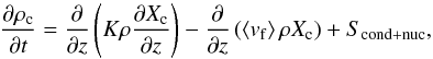 (B.3)where the coagulation/destruction term vanishes because it does not add or remove any mass in the condensed phase of the cloud species. ⟨vf⟩ is the cloud particle mass averaged settling velocity.
For the gas phase of the cloud species, the change in density works out to be  (B.4)where settling of the gas molecule has been neglected; to first order gravity is balanced by the pressure gradient in the atmosphere. To obtain the total density evolution of the cloud species within the atmosphere, we add Eqs. (B.3) and (B.4) to obtain
 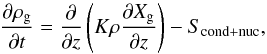 (B.5)For a steady state solution and a net zero mass flux one thus finds that
 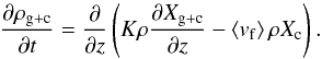 (B.6)which is equal to the equation solved in Ackerman & Marley (2001) except for the fact that they express the settling speed in units of the convective mixing speed.
If one wants to solve for the condensate mass fraction, assuming that the gas mass fraction is known, then one finds from the previous equation that 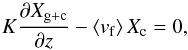 (B.7)In the case of effective heterogeneous nucleation, that is, if the nucleation timescale is shorter than the convective mixing or settling timescale, it can be assumed that Xg is a known quantity:
  (B.8)where Xs is the saturation gas mass fraction and one finds
 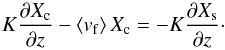 (B.9)In this case Xs can be obtained from an equilibrium chemistry module. For species such as MgSiO3, no gaseous phase exists because the molecule forms through chemical nucleation, therefore ∂Xs/∂z cannot be calculated using equilibrium chemistry. However,
  , that is, the negative gradient of the equilibrium chemistry condensate mass fraction, is a measure for the gas mass gradient between two layers, which arises due to the chemical nucleation of various gaseous species in order to form the condensate (for MgSiO3 it’s Mg(g), SiO(g) and O2(g)). This yields
  (B.10)For species that can exist in the gas phase, and for which the condensation occurs on a small enough spatial range such that the total chemical abundances (gas+solid) are approximately constant, one can assume that
 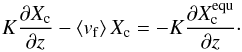 , with
  . This leads to
  , therefore we use Eq. (B.10) in all cases.
A test carried out for a self-luminous planet with Teff = 500 K, set up identically as in Ackerman & Marley (2001), but using our form of the cloud equation as written in Eq. (B.10) yielded very good agreement.
The particle sizes for the clouds are calculated as described in Ackerman & Marley (2001).
All Tables
All Figures
|
Fig. 1 Left panel: our transit candidates in log (g)–Tequ space. See the legend for the meaning of the symbols. Candidates with gray symbols are artificial and have been introduced to fill in the parameter space. “T” and “E” in the legend stand for planets which can be observed in transmission or emission, respectively. The vertical and horizontal lines separate the mostly cloud-free (upper right region) from the potentially cloudy atmospheres (left and bottom regions) as defined in Stevenson (2016). The black, orange, green, and magenta lines show log (g)–Tequ curves of super-Earths and Neptune-like planets (Lopez & Fortney 2014) for the masses and envelope mass fractions as described in the legend. The giant planets which have a gray frame around their name box are not inflated. The upper ends of the vertical orange lines shown for Kepler-13Ab and WASP-18b denote the maximum brightness temperatures observed for these planets. Right panel: planetary mean density as a function of mass. Only the giant planet candidates are plotted here, in the same style as in the left panel. A sample of synthetic, non-inflated planets calculated using the model of Mordasini et al. (2012), Alibert et al. (2013), Jin et al. (2014) is shown as gray crosses. The value of the straight red line shown in the model is a linear function of the planetary mass, as is expected for non-inflated giant planets (see, e.g., Baruteau et al. 2016). |
| In the text | |
|
Fig. 2 Transmission spectra for the warm Saturn HAT-P-12b, along with the observational data taken from Sing et al. (2015a). For clarity, a vertical offset has been applied to the various models. The cloud species considered here are Na2S and KCl only. From top to bottom, the following cases are plotted: a) homogeneous clouds, with a maximum cloud mass fraction of Xmax = 3 × 10⁻⁴·ZPl per species and a single cloud particle size of 0.08 μm. Iron clouds have been neglected; b) like a), but including iron clouds; c) self-consistent clouds using the Ackerman & Marley (2001) model with fsed = 1; d) like c), but using fsed = 0.01; e) clear, fiducial atmospheric model. The colored bars at the bottom of the plot show the spectral range of the various JWST instrument modes. The dotted horizontal lines denote the pressure levels being probed by the transit spectra with the pressure values indicated on the right of the plot. |
| In the text | |
|
Fig. 3 Left panel: the solid lines denote the Na2S cloud-mass fractions as a function of pressure for the fsed = 0.01, 0.3, and 1 models, shown in red, blue, and gray, respectively. The dashed lines denote the mass fractions derived from equilibrium chemistry, that is, in the absence of mixing and settling. For a comparison, the four vertical lines denote the three different Xmax values used in the homogeneous cloud models. Right panel: mean cloud particle radii derived for the fsed = 0.01, 0.3, and 1 cloud models. Again for comparison, the vertical dotted line denotes the particle size a = 0.08μm adopted for the homogeneous cloud models. |
| In the text | |
|
Fig. 4 Synthetic emission spectra of the planets WASP-32b and WASP-10b for the clear fiducial models with solar C/O ratios and for the cases with C/O ratios twice as large as solar. We also plot existing Spitzer photometry for the targets by Garland et al. (2016, WASP-32b) and Kammer et al. (2015, WASP-10b). A dayside-averaged insolation was assumed for both planets. For clarity, both the synthetic spectra and data of WASP-32b have been multiplied by an offset factor of three. |
| In the text | |
|
Fig. 5 Left panel: synthetic transit spectra, observations, and synthetic observations for the planet GJ 1214b. The orange points denote the observational data by Kreidberg et al. (2014), while brown points denote the observational data by Bean et al. (2010), Désert et al. (2011), Bean et al. (2011), Berta et al. (2012), Fraine et al. (2013). Synthetic spectra for the cloudy fsed = 0.3 model (Model 3 in Table 2) are shown as red or purple solid lines for the case including Na2S+KCl clouds or KCl clouds only. The clear model is shown as a teal line. A straight line model is shown as a thick gray solid line. The black dots show the synthetic observations derived for one (top) and ten (bottom) transits, re-binned to a resolution of 50. Vertical offsets have been applied for the sake of clarity. Right panel: p values of the Kolmogorov-Smirnov test for the residuals between the synthetic observation of the Na2S+KCl cloud model and the straight line model fitted to these observations. The p value is shown as a function of Ntransit for the three different instruments of Table 3. For every (instrument, Ntransit) setup, a new straight line model is fitted to the observations. The black dashed line denotes our threshold value of 10-3. |
| In the text | |
|
Fig. 6 Left panel: synthetic transit spectra, observations, and synthetic observations for the planet TrES-4b. Black crosses denote the ground-based observational data by Chan et al. (2011), Sozzetti et al. (2015), Turner et al. (2016). Black squares denote the HST WFC3 data by Ranjan et al. (2014). Synthetic spectra for the homogeneously cloudy models with Xmax = 3 × 10⁻⁴ZPl are shown as teal and red solid lines for the DHS and Mie opacity, respectively. The dashed box at ~10 μm highlights the silicates features due to Mg2SiO4 resonances.The teal and red dots show the corresponding synthetic observations derived for one and ten transits, re-binned to a resolution of 50. Vertical offsets have been applied for the sake of clarity. Right panel: p values of the Kolmogorov-Smirnov test of the residuals between the synthetic observation of the TrES-4b DHS model and the Mie model (solid teal line). The p value is shown as a function of Ntransit for data taken with MIRI LRS considering only the wavelength range of the silicate feature (9–13 μm) and correcting for global model offsets. The dashed teal line shows the p value obtained when analyzing the residuals of the DHS model to its own observation. The black dashed line denotes our threshold value of 10-3. |
| In the text | |
|
Fig. 7 Left panel: synthetic spectra and observational data of the emission spectrum of WASP-18b. A description of the different lines is shown in the legend. The observational data by Nymeyer et al. (2011) are shown as black errorbars. The “emission” lines, which can be made out in the blackbody FPl/F∗ spectrum, are absorption lines of the stellar spectrum. The colored circles show the corresponding Spitzer channels for the synthetic spectra. Right panel: p values of the Kolmogorov-Smirnov test of the residuals between the synthetic observation of the three WASP-18b models and the two respective remaining models. The p value is shown as a function of Ntransit for data taken with the three different instruments listed in Table 3. In order to avoid distinguishing between the models based on offsets, the residual distributions were shifted to have a mean value of 0. The black dashed line denotes our threshold value of 10-3. If an instrument is not shown in one of the three sub-panels then it has a p value lower than 10-12 already after one observation. |
| In the text | |
Current usage metrics show cumulative count of Article Views (full-text article views including HTML views, PDF and ePub downloads, according to the available data) and Abstracts Views on Vision4Press platform.
Data correspond to usage on the plateform after 2015. The current usage metrics is available 48-96 hours after online publication and is updated daily on week days.
Initial download of the metrics may take a while.