| Issue |
A&A
Volume 600, April 2017
|
|
|---|---|---|
| Article Number | A100 | |
| Number of page(s) | 12 | |
| Section | Extragalactic astronomy | |
| DOI | https://doi.org/10.1051/0004-6361/201628400 | |
| Published online | 06 April 2017 | |
Suzaku observations of the merging galaxy cluster Abell 2255: The northeast radio relic
1 SRON Netherlands Institute for Space Research, Sorbonnelaan 2, 3584 CA Utrecht, The Netherlands
e-mail: This email address is being protected from spambots. You need JavaScript enabled to view it.
2 Department of Physics, Nara Women’s University, Kitauoyanishimachi, Nara, 630-8506 Nara, Japan
3 Argelander Institute for Astronomy, Bonn University, Auf dem Hügel 71, 53121 Bonn, Germany
4 Harvard-Smithsonian Center for Astrophysics, 60 Garden Street, Cambridge, MA 02138, USA
5 Department of Earth and Planetary Science, The University of Tokyo, 113-0033 Tokyo, Japan
6 Research Center for the Early Universe, School of Science, The University of Tokyo, 113-0033 Tokyo, Japan
7 Department of Physical Science, Hiroshima University, 1-3-1 Kagamiyama, Higashi-Hiroshima, 739-8526 Hiroshima, Japan
8 Leiden Observatory, Leiden University, PO Box 9513, 2300 RA Leiden, The Netherlands
9 Department of High Energy Astrophysics, Institute of Space and Astronautical Science, 229 Kamagawa, Japan
10 Department of Physics, Graduate School of Science, University of Tokyo, 7-3-1 Hongo, Bunkyo, 113-0033 Tokyo, Japan
11 Department of Physics, Tokyo Metropolitan University, 1-1 Minami-Osawa, Hachioji, 192-0397 Tokyo, Japan
12 Department of Physics, Yamagata University, Kojirakawa-machi 1-4-12, 990-8560 Yamagata, Japan
13 Astronomical Institute Anton Pannekoek, University of Amsterdam, Science Park 904, 1098XH Amsterdam, The Netherlands
14 GRAPPA Institute, University of Amsterdam, 1098 XH Amsterdam, The Netherlands
Received: 28 February 2016
Accepted: 24 November 2016
Abstract
We present the results of deep 140 ks Suzaku X-ray observations of the north-east (NE) radio relic of the merging galaxy cluster Abell 2255. The temperature structure of Abell 2255 is measured out to 0.9 times the virial radius (1.9 Mpc) in the NE direction for the first time. The Suzaku temperature map of the central region suggests a complex temperature distribution, which agrees with previous work. Additionally, on a larger-scale, we confirm that the temperature drops from 6 keV around the cluster center to 3 keV at the outskirts, with two discontinuities at r ~ 5′ (450 kpc) and ~12′ (1100 kpc) from the cluster center. Their locations coincide with surface brightness discontinuities marginally detected in the XMM-Newton image, which indicates the presence of shock structures. From the temperature drop, we estimate the Mach numbers to be ℳinner ~ 1.2 and, ℳouter ~ 1.4. The first structure is most likely related to the large cluster core region (~350–430 kpc), and its Mach number is consistent with the XMM-Newton observation (ℳ ~ 1.24: Sakelliou & Ponman 2006, MNRAS, 367, 1409). Our detection of the second temperature jump, based on the Suzaku key project observation, shows the presence of a shock structure across the NE radio relic. This indicates a connection between the shock structure and the relativistic electrons that generate radio emission. Across the NE radio relic, however, we find a significantly lower temperature ratio (T1/T2 ~ 1.44 ± 0.16 corresponds to ℳX−ray ~ 1.4) than the value expected from radio wavelengths, based on the standard diffusive shock acceleration mechanism (T1/T2> 3.2 or ℳRadio> 2.8). This may suggest that under some conditions, in particular the NE relic of A2255 case, the simple diffusive shock acceleration mechanism is unlikely to be valid, and therefore, more a sophisticated mechanism is required.
Key words: shock waves / galaxies: clusters: intracluster medium / X-rays: galaxies: clusters / galaxies: clusters: individual: Abell 2255 / radio continuum: galaxies
© ESO, 2017
1. Introduction
Abell 2255 (hereafter A2255) is a relatively nearby (z = 0.0806: Struble & Rood 1999) rich merging galaxy cluster. Previous X-ray observations revealed that, the intracluster medium (ICM) has a complex temperature structure, suggesting that A2255 has experienced a recent, violent merger process (David et al. 1993; Davis et al. 2003; Burns et al. 1995; Burns 1998; Feretti et al. 1997; Sakelliou & Ponman 2006). Jones & Forman (1984) found that A2255 has a very large core region (rc ~ 350–430 kpc: see Fig. 4 in their paper), which was confirmed by subsequent observations (Feretti et al. 1997; Sakelliou & Ponman 2006).
The most striking feature of A2255 is the diffuse complex radio emission (Jaffe & Rudnick 1979; Harris et al. 1980; Burns et al. 1995; Feretti et al. 1997; Govoni et al. 2005; Pizzo & de Bruyn 2009). This emission can be roughly classified into two categories: radio halos, and radio relics (see Fig. 5 in Ferrari et al. 2008). Govoni et al. (2005) discovered polarized filamentary radio emission in A2255. Pizzo et al. (2008), Pizzo & de Bruyn (2009) revealed large-scale radio emission at the peripheral regions of the cluster and performed spectral index studies of the radio halo and relic. Information about the spectral index provides important clues concerning the formation process of the radio emission regions. Basic details of the northeast radio relic (hereafter NE relic) are summerized in Table 1. Several mechanisms have been proposed for the origin of the diffuse radio emission, such as turbulence acceleration and hadronic models for radio haloes, and diffusive shock (re-)acceleration (DSA: e.g., Bell 1987, Blandford & Eichler 1987) for radio relics (for details see Brunetti & Jones 2014, and references therein).
Important open questions concerning radio relics include (1) why the Mach numbers of the shock waves inferred from X-ray and radio observation are sometimes inconsistent with each other (e.g., Trasatti et al. 2015; Itahana et al. 2015), and (2) how weak shocks with ℳ < 3 can accelerate particles from thermal pools to relativistic energies via the DSA mechanism (Kang et al. 2012; Pinzke et al. 2013). In some systems, the Mach numbers inferred from X-ray observations clearly violate predictions that are based on a pure DSA theory (Vink & Yamazaki 2014).
Expected shock properties associate with the NE radio relic from radio observation (Pizzo & de Bruyn 2009).
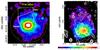 |
Fig. 1 Left: ROSAT image in the 0.1–2.4 keV band of A2255. The white boxes show the FOVs in the Suzaku XIS observations that we discuss in this paper, while the yellow dashed circle shows the virial radius of A2255, r200, corresponding to 23.4′ from the cluster center (see the text for details). Right: background-subtracted Suzaku XIS3 image of A2255 in the 0.5–4.0 keV band smoothed by a two-dimensional Gaussian with σ = 8′′. The image was corrected for exposure time, but not for vignetting. The white contours are 1.0, 2.5, 5.0, 10, 20, 40, 80, and 160 mJy/beam of the WSRT 360 MHz radio intensity (Pizzo & de Bruyn 2009). |
Observation log and exposure time after data screening.
Because X-ray observations enable us to probe ICM properties, a multiwavelength approach is a powerful tool to investigate the origin of the diffuse radio emission. However, because of the off-center location of radio relics in the peripheral regions of the cluster and the corresponding faint ICM emission, it has remained challenging to characterize them at X-ray wavelengths (e.g, Ogrean et al. 2013), except for a few exceptional cases under favorable conditions (e.g., Abell 3667, Abell 115 and El goldo: Finoguenov et al. 2010, Botteon et al. 2016a,b). The Japanese X-ray satellite Suzaku (Mitsuda et al. 2007) improved this situation because of its low and stable background. Suzaku is a suitable observatory to investigate low X-ray surface brightness regions such as cluster peripheries: see Hoshino et al. (2010), Simionescu et al. (2011), Kawaharada et al. (2010), Akamatsu et al. (2011) and Reiprich et al. (2013) for a review. To establish a clear picture of the detailed physical processes associated with radio relics, we conducted deep observations using Suzaku (Suzaku AO9 key project: Akamatsu et al.). In this paper, we report the results of Suzaku X-ray investigations on the NE relic in A2255.
We assume the cosmological parameters H0 = 70 km s-1 Mpc-1, ΩM = 0.27 and ΩΛ = 0.73. With a redshift of z = 0.0806, 1′ corresponds to a diameter of 91.8 kpc. The virial radius, which is represented by r200, is approximately  (1)where E(z) = (ΩM(1 + z)3 + 1−ΩM)1/2 (Henry et al. 2009). For our cosmology and an average temperature of ⟨ kT ⟩ = 6.4 keV (in this work: see Sect. 3.3) r200 = 2.14 Mpc, corresponding to 23.2′. Here, we note that the estimated virial radius is generally consistent with the radius from HIFLUGCS (
 Mpc: Reiprich & Böhringer 2002). For the comparison of the scaled temperature profiles (Sect. 4.1), we adopt the value given by r200 = 2.14 Mpc as the virial radius of A2255. As our fiducial reference for the solar photospheric abundances denoted by Z⊙, we adopt the values reported by Lodders (2003). A Galactic absorption of NH = 2.7 × 1020 cm-2 (Willingale et al. 2013) was included in all fits. Unless otherwise stated, the errors correspond to 68% confidence for each parameter.
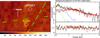 |
Fig. 2 Left: ROSAT R45 (0.47–1.20 keV) band image around A2255 in Galactic coordinates. The two circles (r = 20′) indicate the locations of the A2255 (yellow) and OFFSET (white dashed) observations. Right: NXB-subtracted XIS spectrum of the OFFSET observation. The XIS BI (black) and FI (red) spectra are fitted with the sum of the CXB and the Galactic emission (apec + phabs(apec + powerlaw)). The CXB component is shown as a black curve, and the LHB and MWH emissions are indicated with green and blue curves, respectively. |
2. Observations and data reduction
Suzaku performed two observations: one aimed at the central region and the other at the NE radio relic. Hereafter we refer to these pointings as Center and Relic, respectively (Fig. 1). The X-ray imaging spectrometer (XIS: Koyama et al. 2007) on board Suzaku consists of three front-side illuminated (FI) CCD chips (XIS0, XIS2, and XIS3) and one back-side illuminated (BI) chip (XIS1). After November 9, 2006, XIS2 was no longer operational because of damage from a micrometeoroid strike1. A similar accident occurred on the XIS0 detector2. Because of flooding with a large amount of charges, segment A of XIS1 continuously saturated the analog electronics. For these reasons, we did not use data of XIS0. The segment A of XIS1 was also excluded. All observations were performed with either the normal 5 × 5 or 3 × 3 clocking mode. Data reduction was performed with HEAsoft, version 6.15, XSPEC version 12.8.1, and CALDB version 20140624.
We started with the standard data-screening provided by the Suzaku team and applied event screening with a cosmic-ray cutoff rigidity (COR2) > 6 GV to suppress the detector background. An additional screening for the XIS1 Relic observation data was applied to minimize the detector background. We followed the processes described in the Suzaku XIS official document3.
We used XMM-Newton archival observations (ID:0112260801, 0744410501) for point source identification. We carried out the XMM-Newton EPIC data preparation following Sect. 2.2 in Zhang et al. (2009). The resulting clean exposure times are 9.0 and 25.0 ks, respectively, and are shown in Table 2.
3. Spectral analysis and results
3.1. Spectral analysis approach
For the spectral analysis, we followed our previous approach as described in Akamatsu et al. (2011, 2012a,b). In short, we used the following approach:
-
Estimation of the sky background emission from the cosmicX-ray background (CXB), local hot bubble (LHB) and MilkyWay halo (MWH) using a Suzaku OFFSET observation(Sect. 3.2).
-
Identification of the point sources using XMM-Newton observations and extraction from each Suzaku observation (Sect. 3.2).
-
With this background information, we investigate (i) the global properties of the central region of A2255 (Sect. 3.3) and (ii) the radial temperature profile out to the virial radius (Sect. 3.4).
For the spectrum fitting procedure, we used the XSPEC package version 12.8.1. The spectra of the XIS BI and FI detectors were fitted simultaneously. For the spectral analysis, we generated the redistribution matrix file and ancillary response files assuming a uniform input image (r = 20′) by using xisrmfgen and xisarfgen (Ishisaki et al. 2007) in HEAsoft. The calibration sources were masked using the calmask calibration database file.
Summary of the parameters of the fits for background estimation.
3.2. Background estimation
Radio relics are typically located in cluster peripheries (≥Mpc), where the X-ray emission from the ICM is faint. To investigate the ICM properties of such weak emission, an accurate and proper estimation of the background components is critical. The observed spectrum consists of the emission from the cluster, the celestial emission from non-cluster objects (hereafter sky background) and the detector background (non-X-ray background: NXB).
The sky background mainly comprises three components: LHB (kT ~ 0.1 keV), MWH (kT ~ 0.3 keV) and CXB. To estimate them, we used a nearby Suzaku observation (ID: 800020010, exposure time of ~12 ks after screening), which is located approximately 3° from A2255. Figure 2 (left) shows the ROSAT R45 (0.47–1.20 keV) band image around A2255. Most of the emission in this band is the sky background. Using the HEASARC X-ray Background Tool4, the R45 intensities in the unit of 106 counts/s/arcmin2 are 115.5 ± 2.4 for a r = 30′–60′ ring centered on A2255 and 133.7 ± 5.8 for the offset region (r = 30′ circle), respectively. Thus they agree with each other within about 10%. We extracted spectra from the OFFSET observation and fitted them with a background model:  (2)The redshift and abundance of the two Apec components were fixed at zero and solar, respectively. We used spectra in the range of 0.5–5.0 keV for the BI and FI detectors. The model reproduces the observed spectra well with χ2 = 142.9 with 118 deg of freedom. The resulting best-fit parameters are shown in Table 3, they are in good agreement with the previous study (Takei et al. 2007).
For point-source identification in the Suzaku FOVs, we used XMM-Newton observations. We generated a list of bright point-sources using SAS task edetect_chain applied to five energy bands 0.3–0.5 keV, 0.5–2.0 keV, 2.0–4.5 keV, 4.5–7.5 keV, and 7.5–12 keV using both EPIC pn and MOS data. The point sources are shown as circles with a radius of 25′′ in Fig. 6; this radius was used in the XMM-Newton analysis to estimate the flux of each source.
In the Suzaku analysis, we excluded the point sources with a radius of 1 arcmin to take the point-spread function (PSF) of the Suzaku XRT (Serlemitsos et al. 2007) into account. Additionally, we excluded a bright point-source to the north in the Relic observation with a r = 4′ radius.
In Sect. 3.5, we investigate the impacts of systematic errors associated with the derived background model on the temperature measurement.
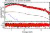 |
Fig. 3 NXB-subtracted spectra of A2255 (r < 5′). The XIS BI (black) and FI (red) spectra are fitted with the ICM model (phabs × Apec), along with the sum of the CXB and Galactic emission. The ICM component is shown with the cyan line. The CXB, LHB and MWH emissions are indicated with black, green, and blue curves, respectively. The sum of all sky background emissions is shown with an orange curve. |
3.3. Global temperature and abundance
First, we investigated the global properties (ICM temperature and abundance) of A2255. We extracted the spectra within r = 5′ of the cluster center ( : Sakelliou & Ponman 2006) and fitted them with an absorbed thin thermal plasma model (phabs × apec) together with the sky background components discussed in the previous section (Sect. 3.2). We kept the temperature and normalization of the ICM component as free parameters and fixed the redshift parameters to 0.0806 (Struble & Rood 1999). The background components were also fixed to their best-fit values obtained in the OFFSET observation. For the fitting, we used the energy range of 0.7–8.0 keV for both detectors. Figure 3 shows the best-fit model. We obtained fairly good fits with χ2 = 1696 with 1657 deg of freedom (red χ2 = 1.03). The best-fit values are listed in Table 4.
Substituting the global temperature of6.37 keV into the σ−T relation (Lubin & Bahcall 1993:σ = 102.52 ± 0.07(kT)0.60 ± 0.11 km s-1), we obtain a velocity dispersion of  , which is consistent with the values estimated by Burns et al. (1995): 1240
 km s-1, Yuan et al. (2003): 1315 ± 86 km s-1 and Zhang et al. (2011): 998 ± 55 km s-1.
To visualize the temperature structure in the central region, we divided the Center observation into 5 × 5 boxes and fitted them in the same manner as described above. Because A2255 is a merging cluster, we do not expect a strong abundance peak in the central region (Matsushita 2011). Therefore, the abundance for the central region was fixed to the global abundance value (0.3 Z⊙) throughout the fitting. The resulting temperature map is shown in Fig. 4. We note that the results are consistent when the abundance is set free. The general observed trend matches previous work (Sakelliou & Ponman 2006): the east region shows somewhat lower temperatures (kT ~ 5 keV) than the west region (kT ~ 7–8 keV).
Best-fit parameters for the central region (r< 5′) of A2255.
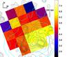 |
Fig. 4 Temperature map of the central region of Abell 2255. The vertical color bar indicates the ICM temperature in units of keV. The lack of data in the four corners is due to the calibration source. The typical error for each box is about ±0.6 keV. The cyan and black contours represent X-ray (XMM-Newton) and radio surface brightness distributions. |
The global temperature (kT = 6.37 ± 0.07 keV) and abundance (Z = 0.28 ± 0.02 Z⊙) agree with most previous studies (EINSTEIN, ASCA, XMM-Newton, and Chandra: David et al. 1993; Ikebe et al. 2002; Sakelliou & Ponman 2006; Cavagnolo et al. 2008). However, ROSAT observations suggest a significantly lower temperature (kT ~ 2–3 keV: Burns et al. 1995; Burns 1998; Feretti et al. 1997) than our results. Sakelliou & Ponman (2006) discussed possible causes for such a disagreement, such as the difference of the source region, energy band, and the possible effect of a multi-temperature plasma. On the other hand, investigations into this disagreement are beyond the scope of this paper.
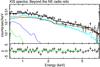 |
Fig. 5 Same as Fig. 3, but beyond the NE radio relic. For clarity, only the BI components are plotted. |
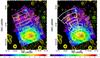 |
Fig. 6 XIS image of A2255. The spectral regions used in the spectral analysis are indicated with the white boxes (2′×10′) (left) and sectors (right). In the left panel, the magenta boxes show the regions used for the pre- and post-shock region. The point sources, identified by XMM-Newton, are highlighted with the green circles (see text for details). |
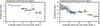 |
Fig. 7 Left: temperature profile of A2255 in the direction from south to NE. Blue and black crosses indicate the best-fit temperature based on the Center and Relic observations, respectively. The dotted gray lines show the profile of the radio emission taken from the WSRT radio data (Pizzo & de Bruyn 2009). The discrepancy between the Center and Relic observations at r = 7′ is due to the lack of the XIS0 data of the Center observation. Right: radial temperature profile of A2255 in the NE radio relic direction. The gray crosses and the dark gray region indicate the radial profiles obtained by XMM-Newton (Sakelliou & Ponman 2006) and Chandra (Cavagnolo et al. 2009), respectively. Green dashed lines show typical systematic changes in the best-fit values that are due to changes in the CXB intensity and NXB level. |
3.4. Radial temperature profile for the NE direction
Flux ratio of the ICM and the sky background components beyond the relic and outermost bins.
To investigate the temperature structure of A2255 toward the NE relic with its radio emission, we extracted 10 boxes (2′ × 10′), as shown in Fig. 6 (left). We followed the same approach as described above, and fixed the abundance to 0.3 Z⊙, which is consistent with the abundance of the central region (previous section) and the measured outskirts of other clusters (Fujita et al. 2008; Werner et al. 2013). We successfully detect the ICM emission beyond the NE radio relic. Table 5 shows the ratio of the ICM and the sky background components at the outer regions. These values are consistent with other clusters (e.g. one could derive the ratio of the ICM and the X-ray background from the right bottom panel of Fig. 2 in Miller et al. 2012). In general, we obtained good fits for all boxes (χ2/ d.o.f.< 1.2). The resulting temperature profile is shown in Fig. 7, where the blue and black crosses indicate the best-fit temperature derived from the Center and Relic observations, respectively. The gray dotted histogram shows the profile of the radio emission taken from the WSRT radio data (Pizzo & de Bruyn 2009). The temperature profile changes from kT ~ 6 keV at the center to ~3 keV beyond the NE radio relic. Furthermore, there are two distinct temperature drops at r = 4′ and 12′, respectively. The latter structure seems to be correlated with the radio relic, which is consistent with other systems (e.g., A3667: Finoguenov et al. 2010, Akamatsu et al. 2012a). In order to estimate the properties of the ICM across the relic, we extracted spectra from the regions indicated by magenta boxes in Fig. 6 (left). We selected the beyond the relic region with 1′ separation to avoid a possible contamination from the bright region. The best-fit values are summarized in Table 7, which are well consistent with the results of box-shaped region. We evaluate the shock properties related to the NE radio relic in the discussion (Sects. 4.1 and 4.2).
To investigate the former structure and radial profile, we extracted spectra by selecting annuli from the center to the periphery as shown in Fig. 6 (right). The radial temperature profile also shows clear discontinuities at r = 5′ and 14′ as shown Fig. 7. In Fig. 7, we compare the Suzaku temperature profile with Chandra (Cavagnolo et al. 2009) and XMM-Newton profiles (Sakelliou & Ponman 2006). Both results covered the central region, where they agree well with the Suzaku result.
3.5. Systematic uncertainty in the temperature measurement
Because the X-ray emission around radio relics is relatively weak, it is important to evaluate the systematic uncertainties in the temperature measurement. First we consider the systematic error of estimating the CXB component in the Relic observation and the detector background. In order to evaluate the uncertainty of the CXB that is due to the statistical fluctuation of the number of point sources, we followed the procedure described in Hoshino et al. (2010). In this paper we refer to the flux limit as 1 × 10-14 erg/s/cm2 determined by XMM-Newton. The resulting CXB fluctuations span 11–27%. We investigate the impact of this systematic effect by changing the intensity by ±11–27% and the normalization of the NXB by ±3% (Tawa et al. 2008).
The resulting best-fit values, after taking into account the systematic errors, are shown with green dashed lines in Fig. 7. The effects of the systematic error that is due to the CXB and NXB are smaller than or compatible to the statistical errors. This result is expected because the regions discussed here are within the virial radius (<0.8r200) and the ICM emission is still comparable to that of the sky background components even around the NE relic (Table 5).
Second, we investigated the effects of flickering pixels. Following the official procedure5, we confirmed that the effect of the flickering pixels was smaller than the statistical error.
Third, because the spatial resolution of the Suzaku telescope is about 2′, the temperature profile is likely to be affected by the choice of region. To study this effect, we shifted the boxes in Fig. 7 (left) by 1.5′ (half of its size) outside and measured the temperature profile again: we found that the temperature ratio across the relic decreased by 20%.
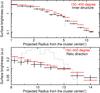 |
Fig. 8 XMM-Newton 0.5–1.4 keV surface brightness profiles (top: inner temperature structure, bottom: across the radio relic). Red and black crosses represent the radial profile of an opening angle with 150°–400° and 80°–130°, respectively. In the top plot, the vertical dashed line indicates the location of the discontinuity. In the bottom plot, the dotted gray lines show WSRT 360 MHz radio emission. |
3.6. Surface brightness structures
In order to investigate whether the observed temperature structures are shocks or cold fronts, we extracted the surface brightness profile from the 0.5–1.4 keV XMM-Newton image in the northeast sector with an opening angle of 80°–130°. The resulting surface brightness profile is shown in the top (the inner structure) and bottom (across the radio relic) panels of Fig. 8. In both panels, black and red crosses represent the radial profiles in the 80°–130° (NE) and 150°–400° sectors, respectively, where we use the latter as the control sector to be compared with the NE sector.
Best-fit parameters for the radial regions.
Best-fit parameters for the pre- and post-shock regions.
In the top panel of Fig. 8, the discontinuity in XMM-Newton surface brightness profile is clearly visible. The location of the discontinuity around r ~ 5.́2, indicated by the dotted gray line, is consistent with that of the inner temperature structure. We found a signature of the surface brightness drop across the relic (r ~ 12.́5). By taking the ratio of the surface brightness across the discontinuity/drop, we estimated the ratio of the electron density C ≡ n2/n1 as CInner = 1.28 ± 0.07 and COuter = 1.32 ± 0.14, respectively. We also found a marginal sign of the inner structure by using the PROFFIT software package (Eckert et al. 2011). We assume that the gas density follows two power-law profiles connecting at a discontinuity with a density jump. In order to derive the best-fit model, the density profile was projected onto the line of sight with the assumption of spherical symmetry. We extracted in the same matter as described above. We obtained the best-fit ratio of the electron density as CInner = 1.33 ± 0.24 with reduced χ2 = 0.53 for 12 d.o.f., which is in good agreement with the above simple estimation. The surface brightness profile and resulting best-fit model are shown in Fig. 9.
Shock properties at the inner and outer structures.
Although the significance is not high enough to claim a firm detection, we consider it is reasonable to think that the inner structure is a shock front (at least not a cold front). For the relic, we were not able to detect a structure across the relic because of poor statistics. Cold fronts at cluster periheries are rare (see Fig. 5 in Walker et al. 2014), and the observed ICM properties across the relic are supportive of the presence of a shock front. Therefore, we conclude that the two temperature structures are shock fronts. We discuss their properties in the following section.
3.7. Constraints on nonthermal emissions
To evaluate the flux of possible nonthermal X-ray emission caused by inverse Compton scattering by the relativistic electrons from the NE relic, we reanalyzed the relic region by adding a power-law component to the ICM model described in the previous subsection. Based on the measured radio spectral index (Pizzo & de Bruyn 2009), we adopted Γrelic = αrelic + 1 = 1.8 (Table 1) as a photon index for the NE relic. As mentioned above, the observed spectra are well modeled with a thermal component. Therefore, we could set an upper limit to the nonthermal emission. The derived one sigma (68%) upper limit of the surface brightness in the 0.3–10 keV is Frelic < 1.8 × 10⁻¹⁴ erg cm-2 s-1 arcmin-2. Assuming the solid angle covered by the NE relic (ΩNE relic = 60 arcmin2, Pizzo & de Bruyn 2009), the upper limit of the flux in the 0.3–10 keV band is <1.0 × 10⁻¹² erg cm-2 s-1. This upper limit is somewhat more stringent than that for the halo (see Fig. 10 in Ota 2012, for a review). The reason for a more stringent upper limit is that for the periphery the lower surface brightness of thermal emission would cause the nonthermal emission to bemore prominent.
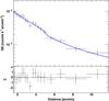 |
Fig. 9 XMM-Newton 2.0–7.0 keV surface brightness profile. The best-fit for the profile is plotted and their residuals are shown in the bottom panel. The inner jump was marginally detected at r = 5.2′ ± 0.6′. |
4. Discussion
The Suzaku observations of the merging galaxy cluster A2255 were conducted out to the virial radius (r200 = 2.14 Mpc or 23.2′). With its deep exposure, it allowed us to investigate the ICM properties beyond the central region. We successfully characterized the ICM temperature profile out to 0.9 times the virial radius. We also confirmed the temperature discontinuities in the NE direction, which indicate shock structures. In the following subsections, we discuss the temperature structure by comparing it to other clusters, evaluate the shock properties, and discuss their implications.
4.1. Shock structures and their properties
Here, we evaluated the Mach number of each shock using the Rankine-Hugoniot jump condition (Landau & Lifshitz 1959) 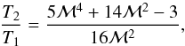 (3)where 1 and 2 denote the pre- and post-shock regions, respectively. We assumed the ratio of specific heats to be γ = 5/3. The estimated Mach numbers are shown in Table 8, with values of ℳinner = 1.27 ± 0.06 and ℳouter = 1.36 ± 0.16. Based on the Mach numbers, we estimated the shock compression parameter to be CInner = 1.40 ± 0.05 and COuter = 1.53 ± 0.23, respectively. These values are consistent with those derived from the surface brightness distributions (Sect. 3.6). Using the measured pre-shock temperature, the sound speeds are cinner ~ 1170 km s-1 and couter ~ 950 km s-1. The shock propagation velocity can be estimated from vshock = cs × ℳ with values of vshock:inner = 1440 ± 50 km s-1 and vshock:outer = 1380 ± 200 km s-1. These shock properties are similar to those observed in other galaxy clusters: Mach number ℳ ~ 1.5–3.0 and shock propagation velocity vshock ~ 1200−3500 km s-1 (Markevitch et al. 2002, 2005; Finoguenov et al. 2010; Macario et al. 2011; Mazzotta et al. 2011; Russell et al. 2012; Dasadia et al. 2016).
4.2. X-ray and radio comparison
Based on the assumption of simple DSA theory, the Mach number can be also estimated from the radio spectral index via  (Drury 1983; Blandford & Eichler 1987). From the observed radio spectral indices (Pizzo & de Bruyn 2009), the expected Mach numbers at the NE relic are ℳ85 cm−2 m> 4.6, ℳ25 cm−85 cm = 2.77 ± 0.35, which are higher than our X-ray result (
 ). Even when the systematic errors estimated in Sect. 3.5 are included, the difference between the Mach numbers inferred from the X-ray and radio observations still holds.
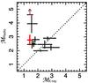 |
Fig. 10 Mach number derived from radio observations (ℳradio) plotted against that from the ICM temperature (ℳX). The results of A2255 are indicated by the red cross (assuming radio spectral index: |


One possible cause of this disagreement is that the Suzaku XRT misses or dilutes the shock-heated region because of its limited spatial resolution (HPD ~ 1.7′: Serlemitsos et al. 2007). This would indicate that the Suzaku XIS spectrum at the post-shock is a multi-temperature plasma consisting of pre- and post-shock media (Sarazin et al. 2014). To confirm this effect, we reanalyzed the post-shock region with a two-temperature (2 kT) model by adding an additional thermal component to the single-temperature model of the post-shock region. However, there is no indication that another thermal component is needed for the post-shock spectrum. The single-temperature model reproduces the measured spectra well (Fig. 5). We note here that it is hard to evaluate the hypothesis of the two-phase plasma with the available X-ray spectra. And as pointed out by Kaastra et al. (2004), the current X-ray spectroscopic capability has its limit on the X-ray diagnostics of the multi-phase plasma. Mazzotta et al. (2004) also demonstrated the difficulties in distinguishing a two-temperature plasma when both temperatures are above 2 keV (see Figs. 1 and 3 in their paper).
Relativistic electrons just behind the shock immediately (within ~ 107 yr) lose their energy via radiative cooling and energy loss via inverse-Compton scattering. Since the cooling timescale of electrons is shorter than the lifetime of the shock, spectral curvature develops, which is called the “aging effect”. As a result, the index of the integrated spectrum decreases at the high-energy end by about 0.5 from αinj for a simple DSA model (αint = αinj−0.5: e.g., Pacholczyk 1970, Miniati 2002). This means that high-quality and spatially resolved low-frequency observations are needed to obtain αinj directly. The number of relics with measured αinj with enough sensitivity and angular resolution is small because of the challenges posed by low-frequency radio observations (e.g., van Weeren et al. 2010, 2012, 2016). For the NE relic in A2255, Pizzo & de Bruyn (2009) confirmed a change in the slope with a different frequency band  and
and  ), indicating the presence of the aging effect. However, their angular resolution is not good enough to resolve the actual spectral index before it affects the aging effect. Therefore, the actual Mach number from the radio observations might be different from what is discussed here.
Although the X-ray photon mixing and radio aging can have some effect, it is still worthwhile to compare the A2255 results with those of other clusters with radio relic. Figure 10 shows a comparison of the Mach number inferred from X-ray and radio observations, which were taken and updated from Akamatsu & Kawahara (2013). The result for the NE relic of A2255 is shown by the red cross together with other objects: CIZA J2242.8+5301 south and north relics (Stroe et al. 2014; Akamatsu et al. 2015), 1RXS J0603.3+4214 (van Weeren et al. 2012; Itahana et al. 2015), A3667 south and north relics (Hindson et al. 2014; Akamatsu et al. 2012a; Akamatsu & Kawahara 2013), A3376 (Kale et al. 2012; Akamatsu et al. 2012b), the Coma relic (Thierbach et al. 2003; Akamatsu et al. 2013) and A2256 (Trasatti et al. 2015). This discrepancy, ℳradio> ℳX, has also been observed for other relics (A2256, Toothbrush, A3667 SE). If this discrepancy is indeed real, it may point to problems in the basic DSA scenario for shocks in clusters. In other words, at least for these objects, the simple DSA assumption does not hold, and therefore, a more complex mechanism might be required. We discuss possible scenarios for this discrepancy in the next subsection.
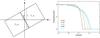 |
Fig. 11 Left: ICM geometry assumed in calculating the projection effect (Sect. 4.4). The ICM temperature Ti, density ni, and line-of-sight path length li are indicated for the pre-shock (i = 1) and post-shock (i = 2) regions. Right: projected temperature profiles against the x-axis for the viewing angles of θ = 15° (black),30° (red),45° (green),60° (blue),and 75° (cyan). |
4.3. Possible scenarios for the discrepancy
Even though Mach numbers from radio and X-ray observations are inconsistent with each other, the expected Mach numbers in clusters are somewhat smaller (ℳ < 5) than those in supernova remnants (ℳ > 1000), which have an efficiency that is high enough to accelerate particles from thermal distributions to the ~TeV regime (e.g., SN1006: Koyama et al. 1995). On the other hand, it is well known that the acceleration efficiency at weak shocks is too low to reproduce the observed radio brightness of radio relics with the DSA mechanism (e.g., Kang et al. 2012; Vink & Yamazaki 2014). To explain these puzzles, several possibilities have been proposed:
-
projection effects that can lead to the underestimation of the Machnumbers from X-ray observations (Skillmanet al. 2013; Honget al. 2015);
-
an underestimation of the post-shock temperature with electrons not reaching thermal equilibrium. Such a phenomenon is observed in SNRs (van Adelsberg et al. 2008; Yamaguchi et al. 2014; Vink et al. 2015);
-
Clumpiness and inhomogeneities in the ICM (Nagai & Lau 2011; Simionescu et al. 2011), which will lead to nonlinearity of the shock-acceleration efficiency (Hoeft & Brüggen 2007);
-
pre-existing low-energy relativistic electrons and/or re-accelerated electrons, resulting in a flat radio spectrum with a rather small temperature jump (Markevitch et al. 2005; Kang et al. 2012; Pinzke et al. 2013; Kang & Ryu 2015; Stroe et al. 2016);
-
a nonuniform Mach number as a results of inhomogeneities in the ICM, which is expected in the periphery of the cluster (Nagai & Lau 2011; Simionescu et al. 2011; Mazzotta et al. 2011);
-
shock-drift accelerations, suggested from particle-in-cell simulations (Guo et al. 2014a,b);
-
other mechanisms, for instance turbulence accelerations (e.g., Fujita et al. 2015, 2016).
Based on our X-ray observational results, we discuss some of the above possibilities.
– Ion-electron non-equilibrium after shock heating:
shocks not only work for particle acceleration, but also for heating. Immediately after shock heating, an electron-ion two-temperature structure has been predicted based on numerical simulations (Takizawa 1999; Akahori & Yoshikawa 2010). This could lead to an underestimation of the post-shock temperature because it is hard to constrain the ion temperature with current X-ray satellites and instruments. Therefore, the main observable is the electron temperature of the ICM, which will reach temperature equilibrium with the ion after the ion-electron relaxation time after shock heating. With assumption of the energy transportation from ions to electrons through Coulomb collisions, the ion-electron relaxation time can be estimated as 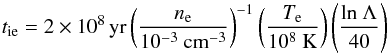 (4)(Takizawa 1999). Here, ln Λ denotes the Coulomb logarithm (Spitzer 1956). From the APEC normalization, we estimated the electron density at the post-shock region as ne ~ 3 × 10⁻⁴ cm-3, assuming a line-of-sight length of 1 Mpc. Using an electron density of ne = 3 × 10⁻⁴ cm-3 and Te = 4.9 keV at the post-shock region, we expect the ion-electron relaxation time to be ti.e. = 0.3 × 10⁹ yr. The speed of the post-shock material relative to the shock is v2 = vs/C ~ 840 km s-1. Thus, the region where the electron temperature is much lower than the ion temperature is about di.e. = ti.e. × v2 = 250 kpc. If there is no projection effect, then the estimated value is consistent with the integrated region that is used in the spectral analysis. This indicates that the ion-electron non-equilibration could be a possible cause of the discrepancy. We note that there are several claims that electrons can be more rapidly energized (so-called instant equilibration) than by Coulomb collisions (Markevitch 2010; Yamaguchi et al. 2014). However, it is difficult to investigate this phenomenon without better spectra than those from the current X-ray spectrometer. The upcoming Athena satellite can shed new light on this problem.
– Projection effects:
since it is difficult to accurately estimate the projection effects on the ℳX measurement, we calculate the temperature profiles to be obtained from X-ray spectroscopy under some simplified conditions. As shown in the left panel of Fig. 11, we consider a pre-shock (T1 = 2 keV) gas and a post-shock (T2 = 6 keV) gas in (5′)3 cubes whose density ratio is n2/n1 = 3 since the radio observation indicates a ℳ ~ 3 shock (Table 1). Assuming that the emission spectrum is given by a superposition of two APEC models and the emission measure of each model is proportional to  , we simulate the total XIS spectrum at a certain x by the XSPEC fakeit command and fit it by a single-component APEC model. The right panel of Fig. 11 shows the resulting temperature profile against the x-axis for the viewing angles of θ = 15°, 30°, 45°, 60°,and 75°. Here the step-size was
  , and 40 regions were simulated to produce the temperature profile for each viewing angle. This result indicates that the temperature of the pre-shock gas is easily overestimated as a consequence of the superposition of the hotter emission while the post-shock gas temperature is less affected. This result is consistent with the predictions by Skillman et al. (2013) and Hong et al. (2015). Thus the observed temperature ratio is likely to be reproduced when θ ≳ 30°.
Next, we estimate the viewing angle based on the line-of-sight galaxy velocity distribution (Yuan et al. 2003) assuming that these galaxies in the infalling subcluster are move together with the shock front. Because the brightest galaxy at the NE relic has a redshift of 0.0845, the peculiar velocity of the subcluster relative to the main cluster (0.0806: Struble & Rood 1999) is roughly estimated as 1180 km s-1, yielding θ = arctan(vpec/vs) = arctan(1180/1380) = 40.5°. This also suggests that the projection effect is not negligible in the present ℳX estimation. Our present simulation is based on the simplified conditions, however and is not accurate enough to reproduce the temperature observed at the outermost region where the projection effects are expected to be small. From the right panel of Fig. 11, in case of the view angle of 40.5°, next to the shock (r = 0.0′–2.0′) is expected to have a temperature higher than the outermost bin. On the other hand, the observed temperature in the outermost region ( keV) is consistent with that derived being located at immediately beyond the relic (
 keV). This indicates that either the viewing angle is overestimated or the simulation is too simple. To address this problem, X-ray observations with better spatial and spectral resolutions are required.
– Clumpiness and inhomogeneities in the ICM:
Nagai & Lau (2011) suggested that the ICM at the cluster peripheral regions is not a single phase, meaning that it cannnot be characterized by a single temperature and gas density, because of a clumpy accretion flow from large-scale structures. The degree of clumpiness of the ICM is charcterized by a clumping factor C ≡ ⟨ ρ2 ⟩ / ⟨ ρ ⟩ 2. Here, C = 1 represents a clump-free ICM. Simionescu et al. (2011) reported the possibility of a high clumpiness factor (10–20) at the virial radius based on Suzaku observations of the Perseus cluster. The inhomogeneities of the ICM generate a non-uniform Mach number, which could lead to the disagreement of shock properties inferred from X-ray and radio observations because the shock acceleration efficiency strongly nonlinearly depends on the Mach number (Hoeft & Brüggen 2007). However, in the A2255, the NE relic is located well inside of the virial radius at ~0.6 r200. The simulations (Nagai & Lau 2011) predict that the clumping factor at r = 0.5r200 is almost unity and gradually increases to the virial radius (C ~ 2). Therefore, clumping is not likely to be the dominant source of the discrepancy.
4.4. Magnetic fields at the NE relic
The diffuse radio emission is expected to be generated by synchrotron radiation of GeV energy electrons with a magnetic field in the ICM. These electrons scatter CMB photons via the inverse-Compton scattering. The nonthermal emission from clusters is a useful tool to investigate the magnetic field in the ICM. Assuming that the same population of relativistic electrons radiates synchrotron emission and scatters off the CMB photons, the magnetic field in the ICM can be estimated by using the following equations for the synchrotron emission at the frequency νSyn and the inverse-Compton emission at νIC (Blumenthal & Gould 1970) 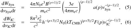 where N0 and p are the normalization and the power-law index of the electron distribution, r0 is the classical electron radius, h is the Planck constant, TCMB is CMB temperature, and TCMB = 2.73(1 + z) K. The magnetic field in the cluster can be estimated by substituting observed flux densities of the synchrotron emission SSyn and the inverse-Compton X-ray emission SIC as well as their frequencies νSyn and νIC by the relation SSyn/SIC = (dWSyn/ dνSyndt)/(dWIC/ dνICdt) (see also Ferrari et al. 2008; Ota et al. 2008, 2014).
Based on the X-ray spectral analysis assuming Γrelic = 1.8 for the nonthermal power-law component (Sect. 3.7), we derive the upper limit on the IC flux density as SIC< 0.067 mJy at 2 keV (νIC = 2.9 × 10¹⁸ Hz). Combining this limit with the radio flux density of the NE relic, SSyn = 117 mJy at νSyn = 328 MHz (Pizzo & de Bruyn 2009), we obtain the lower limit of the magnetic field to be B> 0.0024 μG. Although the value depends on the assumptions, e.g., such as spectral modeling and area of the NE radio relic, the estimated lower limit is still much lower than the equipartition magnetic field (Beq = 0.4 μG) based on radio observations (Pizzo & de Bruyn 2009). A hard X-ray observation with higher sensitivity is needed to improve the accuracy and test the equipartition estimation (e.g., Bartels et al. 2015).
5. Summary
Based on deep Suzaku observations of A2255 (z = 0.0806), we determined the radial distribution of the ICM temperature out to 0.9r200. We found two temperature discontinuities at r = 5′ and 12′, whose locations coincide with the surface brightness drops observed in the XMM-Newton image. Thus these structures can be interpreted as shock fronts. We estimated their Mach numbers, ℳinner ~ 1.2 and ℳouter ~ 1.4 using the Rankine-Hugoniot jump condition. The Mach number of the inner shock is consistent with the previous XMM-Newton result (Sakelliou & Ponman 2006), but for the different azimuthal directions. Thus the western shock structures reported by XMM-Newton and the northern structure detected by Suzaku might originate from the same episode of a subcluster infall. To examine this, we need a detailed investigation of the thermal properties of the ICM in other directions, which is to be presented in our forthcoming paper. The location of the second shock front coincides with that of the NE relic, indicating that the electrons in the NE relic have been accelerated by a merger shock. However, the Mach numbers derived from X-ray and radio observations, assuming basic DSA mechanism, are inconsistent with each other. This indicates that the simple DSA mechanism is not valid under some conditions, and therefore, more sophisticated mechanisms are required.
Acknowledgments
We are grateful to the referee for useful comments that helped to improve this paper. The authors thank the Suzaku team members for their support on the Suzaku project, R. Pizzo for providing the WSRT radio images. H.A and F.Z. acknowledge the support of NWO via a Veni grant. Y.Y.Z. acknowledges support by the German BMWi through the Verbundforschung under grant 50 OR 1506. R.J.W. is supported by a Clay Fellowship awarded by the Harvard-Smithsonian Center for Astrophysics. N.O. and M.T. acknowledge support by a Grant-in-Aid by KAKENHI No.25400231 and 26400218. SRON is supported financially by NWO, the Netherlands Organization for Scientific Research.
References
- Akahori, T., & Yoshikawa, K. 2010, PASJ, 62, 335 [NASA ADS] [Google Scholar]
- Akamatsu, H., & Kawahara, H. 2013, PASJ, 65, 16 [NASA ADS] [CrossRef] [Google Scholar]
- Akamatsu, H., Hoshino, A., Ishisaki, Y., et al. 2011, PASJ, 63, 1019 [NASA ADS] [Google Scholar]
- Akamatsu, H., de Plaa, J., Kaastra, J., et al. 2012a,PASJ, 64, 49 [Google Scholar]
- Akamatsu, H., Takizawa, M., Nakazawa, K., et al. 2012b,PASJ, 64, 67 [Google Scholar]
- Akamatsu, H., Inoue, S., Sato, T., et al. 2013, PASJ, 65, 89 [NASA ADS] [Google Scholar]
- Akamatsu, H., van Weeren, R. J., Ogrean, G. A., et al. 2015, A&A, 582, A87 [Google Scholar]
- Bartels, R., Zandanel, F., & Ando, S. 2015, A&A, 582, A20 [Google Scholar]
- Bell, A. R. 1987, MNRAS, 225, 615 [NASA ADS] [Google Scholar]
- Blandford, R., & Eichler, D. 1987, Phys. Rep., 154, 1 [Google Scholar]
- Botteon, A., Gastaldello, F., Brunetti, G., & Dallacasa, D. 2016a, MNRAS, 460, L84 [NASA ADS] [CrossRef] [Google Scholar]
- Botteon, A., Gastaldello, F., Brunetti, G., & Kale, R. 2016b, MNRAS, 463, 1534 [NASA ADS] [CrossRef] [Google Scholar]
- Brunetti, G., & Jones, T. W. 2014, Int. J. Mod. Phys. D, 23, 30007 [Google Scholar]
- Burns, J. O. 1998, Science, 280, 400 [NASA ADS] [CrossRef] [Google Scholar]
- Burns, J. O., Roettiger, K., Pinkney, J., et al. 1995, ApJ, 446, 583 [NASA ADS] [CrossRef] [Google Scholar]
- Cavagnolo, K. W., Donahue, M., Voit, G. M., & Sun, M. 2008, ApJ, 682, 821 [NASA ADS] [CrossRef] [Google Scholar]
- Cavagnolo, K. W., Donahue, M., Voit, G. M., & Sun, M. 2009, ApJS, 182, 12 [NASA ADS] [CrossRef] [Google Scholar]
- Dasadia, S., Sun, M., Sarazin, C., et al. 2016, ApJ, 820, L20 [Google Scholar]
- David, L. P., Slyz, A., Jones, C., et al. 1993, ApJ, 412, 479 [NASA ADS] [CrossRef] [Google Scholar]
- Davis, D. S., Miller, N. A., & Mushotzky, R. F. 2003, ApJ, 597, 202 [NASA ADS] [CrossRef] [EDP Sciences] [Google Scholar]
- Drury, L. O. 1983, Rep. Progr. Phys., 46, 973 [Google Scholar]
- Eckert, D., Molendi, S., & Paltani, S. 2011, A&A, 526, A79 [NASA ADS] [CrossRef] [EDP Sciences] [Google Scholar]
- Feretti, L., Boehringer, H., Giovannini, G., & Neumann, D. 1997, A&A, 317, 432 [NASA ADS] [Google Scholar]
- Ferrari, C., Govoni, F., Schindler, S., Bykov, A. M., & Rephaeli, Y. 2008, Space Sci. Rev., 134, 93 [NASA ADS] [CrossRef] [Google Scholar]
- Finoguenov, A., Sarazin, C. L., Nakazawa, K., Wik, D. R., & Clarke, T. E. 2010, ApJ, 715, 1143 [NASA ADS] [CrossRef] [Google Scholar]
- Fujita, Y., Tawa, N., Hayashida, K., et al. 2008, PASJ, 60, S343 [NASA ADS] [CrossRef] [Google Scholar]
- Fujita, Y., Takizawa, M., Yamazaki, R., Akamatsu, H., & Ohno, H. 2015, ApJ, 815, 116 [NASA ADS] [CrossRef] [Google Scholar]
- Fujita, Y., Akamatsu, H., & Kimura, S. S. 2016, PASJ, 68, 34 [NASA ADS] [CrossRef] [Google Scholar]
- Govoni, F., Murgia, M., Feretti, L., et al. 2005, A&A, 430, L5 [NASA ADS] [CrossRef] [EDP Sciences] [Google Scholar]
- Guo, X., Sironi, L., & Narayan, R. 2014a, ApJ, 794, 153 [NASA ADS] [CrossRef] [Google Scholar]
- Guo, X., Sironi, L., & Narayan, R. 2014b, ApJ, 797, 47 [NASA ADS] [CrossRef] [Google Scholar]
- Harris, D. E., Kapahi, V. K., & Ekers, R. D. 1980, A&AS, 39, 215 [NASA ADS] [Google Scholar]
- Henry, J. P., Evrard, A. E., Hoekstra, H., Babul, A., & Mahdavi, A. 2009, ApJ, 691, 1307 [NASA ADS] [CrossRef] [Google Scholar]
- Hindson, L., Johnston-Hollitt, M., Hurley-Walker, N., et al. 2014, MNRAS, 445, 330 [NASA ADS] [CrossRef] [Google Scholar]
- Hoeft, M., & Brüggen, M. 2007, MNRAS, 375, 77 [NASA ADS] [CrossRef] [Google Scholar]
- Hong, S. E., Kang, H., & Ryu, D. 2015, ApJ, 812, 49 [NASA ADS] [CrossRef] [Google Scholar]
- Hoshino, A., Henry, J. P., Sato, K., et al. 2010, PASJ, 62, 371 [NASA ADS] [CrossRef] [Google Scholar]
- Ikebe, Y., Reiprich, T. H., Böhringer, H., Tanaka, Y., & Kitayama, T. 2002, A&A, 383, 773 [NASA ADS] [CrossRef] [EDP Sciences] [Google Scholar]
- Ishisaki, Y., Maeda, Y., Fujimoto, R., et al. 2007, PASJ, 59, 113 [NASA ADS] [Google Scholar]
- Itahana, M., Takizawa, M., Akamatsu, H., et al. 2015, PASJ [Google Scholar]
- Jaffe, W. J., & Rudnick, L. 1979, ApJ, 233, 453 [NASA ADS] [CrossRef] [Google Scholar]
- Jones, C., & Forman, W. 1984, ApJ, 276, 38 [NASA ADS] [CrossRef] [Google Scholar]
- Kaastra, J. S., Tamura, T., Peterson, J. R., et al. 2004, A&A, 413, 415 [NASA ADS] [CrossRef] [EDP Sciences] [Google Scholar]
- Kale, R., Dwarakanath, K. S., Bagchi, J., & Paul, S. 2012, MNRAS, 426, 1204 [NASA ADS] [CrossRef] [Google Scholar]
- Kang, H., & Ryu, D. 2015, ApJ, 809, 186 [NASA ADS] [CrossRef] [Google Scholar]
- Kang, H., Ryu, D., & Jones, T. W. 2012, ApJ, 756, 97 [Google Scholar]
- Kawaharada, M., Okabe, N., Umetsu, K., et al. 2010, ApJ, 714, 423 [NASA ADS] [CrossRef] [Google Scholar]
- Koyama, K., Petre, R., Gotthelf, E. V., et al. 1995, Nature, 378, 255 [NASA ADS] [CrossRef] [Google Scholar]
- Koyama, K., Tsunemi, H., Dotani, T., et al. 2007, PASJ, 59, 23 [Google Scholar]
- Kushino, A., Ishisaki, Y., Morita, U., et al. 2002, PASJ, 54, 327 [NASA ADS] [CrossRef] [Google Scholar]
- Landau, L. D., & Lifshitz, E. M. 1959, Fluid mechanics, Course of theoretical physics (Oxford: Pergamon Press) [Google Scholar]
- Lodders, K. 2003, ApJ, 591, 1220 [NASA ADS] [CrossRef] [Google Scholar]
- Lubin, L. M., & Bahcall, N. A. 1993, ApJ, 415, L17 [NASA ADS] [CrossRef] [Google Scholar]
- Macario, G., Markevitch, M., Giacintucci, S., et al. 2011, ApJ, 728, 82 [NASA ADS] [CrossRef] [Google Scholar]
- Markevitch, M. 2010, ArXiv e-prints [arXiv:1010.3660] [Google Scholar]
- Markevitch, M., Gonzalez, A. H., David, L., et al. 2002, ApJ, 567, L27 [NASA ADS] [CrossRef] [Google Scholar]
- Markevitch, M., Govoni, F., Brunetti, G., & Jerius, D. 2005, ApJ, 627, 733 [NASA ADS] [CrossRef] [Google Scholar]
- Matsushita, K. 2011, A&A, 527, A134 [NASA ADS] [CrossRef] [EDP Sciences] [Google Scholar]
- Mazzotta, P., Rasia, E., Moscardini, L., & Tormen, G. 2004, MNRAS, 354, 10 [NASA ADS] [CrossRef] [Google Scholar]
- Mazzotta, P., Bourdin, H., Giacintucci, S., Markevitch, M., & Venturi, T. 2011, Mem. Soc. Astron. It., 82, 495 [NASA ADS] [Google Scholar]
- Miller, E. D., Bautz, M., George, J., et al. 2012, in AIP Conf. Ser. 1427, eds. R. Petre, K. Mitsuda, & L. Angelini, 13 [Google Scholar]
- Miniati, F. 2002, MNRAS, 337, 199 [NASA ADS] [CrossRef] [Google Scholar]
- Mitsuda, K., Bautz, M., Inoue, H., et al. 2007, PASJ, 59, 1 [Google Scholar]
- Nagai, D., & Lau, E. T. 2011, ApJ, 731, L10 [NASA ADS] [CrossRef] [Google Scholar]
- Ogrean, G. A., Brüggen, M., Röttgering, H., et al. 2013, MNRAS, 429, 2617 [NASA ADS] [CrossRef] [Google Scholar]
- Ota, N. 2012, RA&A, 12, 973 [Google Scholar]
- Pacholczyk, A. G. 1970, Radio astrophysics. Nonthermal processes in galactic and extragalactic sources (San Francisco: Freeman) [Google Scholar]
- Pinzke, A., Oh, S. P., & Pfrommer, C. 2013, MNRAS, 435, 1061 [NASA ADS] [CrossRef] [Google Scholar]
- Pizzo, R. F., & de Bruyn, A. G. 2009, A&A, 507, 639 [NASA ADS] [CrossRef] [EDP Sciences] [Google Scholar]
- Pizzo, R. F., de Bruyn, A. G., Feretti, L., & Govoni, F. 2008, A&A, 481, L91 [NASA ADS] [CrossRef] [EDP Sciences] [Google Scholar]
- Reiprich, T. H., & Böhringer, H. 2002, ApJ, 567, 716 [NASA ADS] [CrossRef] [Google Scholar]
- Reiprich, T. H., Basu, K., Ettori, S., et al. 2013, Space Sci. Rev., 177, 195 [NASA ADS] [CrossRef] [EDP Sciences] [Google Scholar]
- Russell, H. R., McNamara, B. R., Sanders, J. S., et al. 2012, MNRAS, 423, 236 [NASA ADS] [CrossRef] [Google Scholar]
- Sakelliou, I., & Ponman, T. J. 2006, MNRAS, 367, 1409 [NASA ADS] [CrossRef] [Google Scholar]
- Sarazin, C., Hogge, T., Chatzikos, M., et al. 2014, in The X-ray Universe 2014, ed. J.-U. Ness, 181 [Google Scholar]
- Serlemitsos, P. J., Soong, Y., Chan, K.-W., et al. 2007, PASJ, 59, 9 [Google Scholar]
- Simionescu, A., Allen, S. W., Mantz, A., et al. 2011, Science, 331, 1576 [NASA ADS] [CrossRef] [Google Scholar]
- Skillman, S. W., Xu, H., Hallman, E. J., et al. 2013, ApJ, 765, 21 [NASA ADS] [CrossRef] [Google Scholar]
- Spitzer, L. 1956, Physics of Fully Ionized Gases (New York: Interscience Publishers) [Google Scholar]
- Stroe, A., Harwood, J. J., Hardcastle, M. J., & Röttgering, H. J. A. 2014, MNRAS, 445, 1213 [NASA ADS] [CrossRef] [Google Scholar]
- Stroe, A., Shimwell, T., Rumsey, C., et al. 2016, MNRAS, 455, 2402 [NASA ADS] [CrossRef] [Google Scholar]
- Struble, M. F., & Rood, H. J. 1999, ApJS, 125, 35 [NASA ADS] [CrossRef] [Google Scholar]
- Takei, Y., Ohashi, T., Henry, J. P., et al. 2007, PASJ, 59, 339 [NASA ADS] [CrossRef] [Google Scholar]
- Takizawa, M. 1999, ApJ, 520, 514 [NASA ADS] [CrossRef] [Google Scholar]
- Tawa, N., Hayashida, K., Nagai, M., et al. 2008, PASJ, 60, 11 [Google Scholar]
- Thierbach, M., Klein, U., & Wielebinski, R. 2003, A&A, 397, 53 [NASA ADS] [CrossRef] [EDP Sciences] [Google Scholar]
- Trasatti, M., Akamatsu, H., Lovisari, L., et al. 2015, A&A, 575, A45 [NASA ADS] [CrossRef] [EDP Sciences] [Google Scholar]
- van Adelsberg, M., Heng, K., McCray, R., & Raymond, J. C. 2008, ApJ, 689, 1089 [CrossRef] [Google Scholar]
- van Weeren, R. J., Röttgering, H. J. A., Brüggen, M., & Hoeft, M. 2010, Science, 330, 347 [NASA ADS] [CrossRef] [PubMed] [Google Scholar]
- van Weeren, R. J., Röttgering, H. J. A., Intema, H. T., et al. 2012, A&A, 546, A124 [NASA ADS] [CrossRef] [EDP Sciences] [Google Scholar]
- van Weeren, R. J., Brunetti, G., Brüggen, M., et al. 2016, ApJ, 818, 204 [NASA ADS] [CrossRef] [Google Scholar]
- Vink, J., & Yamazaki, R. 2014, ApJ, 780, 125 [NASA ADS] [CrossRef] [Google Scholar]
- Vink, J., Broersen, S., Bykov, A., & Gabici, S. 2015, A&A, 579, A13 [NASA ADS] [CrossRef] [EDP Sciences] [Google Scholar]
- Walker, S. A., Fabian, A. C., & Sanders, J. S. 2014, MNRAS, 441, L31 [NASA ADS] [CrossRef] [Google Scholar]
- Werner, N., Urban, O., Simionescu, A., & Allen, S. W. 2013, Nature, 502, 656 [NASA ADS] [CrossRef] [Google Scholar]
- Willingale, R., Starling, R. L. C., Beardmore, A. P., Tanvir, N. R., & O’Brien, P. T. 2013, MNRAS, 431, 394 [NASA ADS] [CrossRef] [Google Scholar]
- Yamaguchi, H., Eriksen, K. A., Badenes, C., et al. 2014, ApJ, 780, 136 [NASA ADS] [CrossRef] [Google Scholar]
- Yuan, Q., Zhou, X., & Jiang, Z. 2003, ApJS, 149, 53 [NASA ADS] [CrossRef] [Google Scholar]
- Zhang, Y.-Y., Reiprich, T. H., Finoguenov, A., Hudson, D. S., & Sarazin, C. L. 2009, ApJ, 699, 1178 [NASA ADS] [CrossRef] [Google Scholar]
- Zhang, Y.-Y., Andernach, H., Caretta, C. A., et al. 2011, A&A, 526, A105 [NASA ADS] [CrossRef] [EDP Sciences] [Google Scholar]
All Tables
Expected shock properties associate with the NE radio relic from radio observation (Pizzo & de Bruyn 2009).
Flux ratio of the ICM and the sky background components beyond the relic and outermost bins.
All Figures
|
Fig. 1 Left: ROSAT image in the 0.1–2.4 keV band of A2255. The white boxes show the FOVs in the Suzaku XIS observations that we discuss in this paper, while the yellow dashed circle shows the virial radius of A2255, r200, corresponding to 23.4′ from the cluster center (see the text for details). Right: background-subtracted Suzaku XIS3 image of A2255 in the 0.5–4.0 keV band smoothed by a two-dimensional Gaussian with σ = 8′′. The image was corrected for exposure time, but not for vignetting. The white contours are 1.0, 2.5, 5.0, 10, 20, 40, 80, and 160 mJy/beam of the WSRT 360 MHz radio intensity (Pizzo & de Bruyn 2009). |
| In the text | |
|
Fig. 2 Left: ROSAT R45 (0.47–1.20 keV) band image around A2255 in Galactic coordinates. The two circles (r = 20′) indicate the locations of the A2255 (yellow) and OFFSET (white dashed) observations. Right: NXB-subtracted XIS spectrum of the OFFSET observation. The XIS BI (black) and FI (red) spectra are fitted with the sum of the CXB and the Galactic emission (apec + phabs(apec + powerlaw)). The CXB component is shown as a black curve, and the LHB and MWH emissions are indicated with green and blue curves, respectively. |
| In the text | |
|
Fig. 3 NXB-subtracted spectra of A2255 (r < 5′). The XIS BI (black) and FI (red) spectra are fitted with the ICM model (phabs × Apec), along with the sum of the CXB and Galactic emission. The ICM component is shown with the cyan line. The CXB, LHB and MWH emissions are indicated with black, green, and blue curves, respectively. The sum of all sky background emissions is shown with an orange curve. |
| In the text | |
|
Fig. 4 Temperature map of the central region of Abell 2255. The vertical color bar indicates the ICM temperature in units of keV. The lack of data in the four corners is due to the calibration source. The typical error for each box is about ±0.6 keV. The cyan and black contours represent X-ray (XMM-Newton) and radio surface brightness distributions. |
| In the text | |
|
Fig. 5 Same as Fig. 3, but beyond the NE radio relic. For clarity, only the BI components are plotted. |
| In the text | |
|
Fig. 6 XIS image of A2255. The spectral regions used in the spectral analysis are indicated with the white boxes (2′×10′) (left) and sectors (right). In the left panel, the magenta boxes show the regions used for the pre- and post-shock region. The point sources, identified by XMM-Newton, are highlighted with the green circles (see text for details). |
| In the text | |
|
Fig. 7 Left: temperature profile of A2255 in the direction from south to NE. Blue and black crosses indicate the best-fit temperature based on the Center and Relic observations, respectively. The dotted gray lines show the profile of the radio emission taken from the WSRT radio data (Pizzo & de Bruyn 2009). The discrepancy between the Center and Relic observations at r = 7′ is due to the lack of the XIS0 data of the Center observation. Right: radial temperature profile of A2255 in the NE radio relic direction. The gray crosses and the dark gray region indicate the radial profiles obtained by XMM-Newton (Sakelliou & Ponman 2006) and Chandra (Cavagnolo et al. 2009), respectively. Green dashed lines show typical systematic changes in the best-fit values that are due to changes in the CXB intensity and NXB level. |
| In the text | |
|
Fig. 8 XMM-Newton 0.5–1.4 keV surface brightness profiles (top: inner temperature structure, bottom: across the radio relic). Red and black crosses represent the radial profile of an opening angle with 150°–400° and 80°–130°, respectively. In the top plot, the vertical dashed line indicates the location of the discontinuity. In the bottom plot, the dotted gray lines show WSRT 360 MHz radio emission. |
| In the text | |
|
Fig. 9 XMM-Newton 2.0–7.0 keV surface brightness profile. The best-fit for the profile is plotted and their residuals are shown in the bottom panel. The inner jump was marginally detected at r = 5.2′ ± 0.6′. |
| In the text | |
|
Fig. 10 Mach number derived from radio observations (ℳradio) plotted against that from the ICM temperature (ℳX). The results of A2255 are indicated by the red cross (assuming radio spectral index: |
| In the text | |
|
Fig. 11 Left: ICM geometry assumed in calculating the projection effect (Sect. 4.4). The ICM temperature Ti, density ni, and line-of-sight path length li are indicated for the pre-shock (i = 1) and post-shock (i = 2) regions. Right: projected temperature profiles against the x-axis for the viewing angles of θ = 15° (black),30° (red),45° (green),60° (blue),and 75° (cyan). |
| In the text | |
Current usage metrics show cumulative count of Article Views (full-text article views including HTML views, PDF and ePub downloads, according to the available data) and Abstracts Views on Vision4Press platform.
Data correspond to usage on the plateform after 2015. The current usage metrics is available 48-96 hours after online publication and is updated daily on week days.
Initial download of the metrics may take a while.