| Issue |
A&A
Volume 598, February 2017
|
|
|---|---|---|
| Article Number | A43 | |
| Number of page(s) | 10 | |
| Section | Interstellar and circumstellar matter | |
| DOI | https://doi.org/10.1051/0004-6361/201629145 | |
| Published online | 27 January 2017 | |
Constraining the mass of the planet(s) sculpting a disk cavity
The intriguing case of 2MASS J16042165-2130284⋆,⋆⋆
1 Departamento de Física Teórica, Universidad Autónoma de Madrid, Cantoblanco, 28049 Madrid, Spain
e-mail: hector.canovas@uam.es
2 Departamento de Física y Astronomía, Universidad de Valparaíso, Valparaíso, Chile
3 Facultad de Ingeniería, Universidad Diego Portales, Av. Ejercito 441, 1058 Santiago, Chile
4 European Southern Observatory, 3107 Alonso de Cordova, Vitacura, 1058 Santiago, Chile
5 Aix Marseille Université, CNRS, LAM (Laboratoire d’Astrophysique de Marseille) UMR 7326, 13388, Marseille, France
6 CNRS, IPAG, 38000 Grenoble, France
7 Univ. Grenoble Alpes, IPAG, 38000 Grenoble, France
8 Departamento de Ciencias Fisicas, Facultad de Ciencias Exactas, Universidad Andres Bello. Av. Fernandez Concha 700, Las Condes, Santiago, Chile
9 Millennium Nucleus “Protoplanetary Disks in ALMA Early Science”, 1058 Santiago, Chile
Received: 18 June 2016
Accepted: 7 October 2016
Context. The large cavities observed in the dust and gas distributions of transition disks may be explained by planet-disk interactions. At ~ 145 pc, 2MASS J16042165-2130284 (J1604) is a 5–12 Myr old transitional disk with different gap sizes in the mm- and μm-sized dust distributions (outer edges at ~ 79 and at ~ 63 au, respectively). Its 12CO emission shows a ~ 30 au cavity. This radial structure suggests that giant planets are sculpting this disk.
Aims. We aim to constrain the masses and locations of plausible giant planets around J1604.
Methods. We observed J1604 with the Spectro-Polarimetric High-contrast Exoplanet REsearch (SPHERE) at the Very Large Telescope (VLT), in IRDIFS_EXT, pupil-stabilized mode, obtaining YJH-band images with the integral field spectrograph (IFS) and K1K2-band images with the Infra-Red Dual-beam Imager and Spectrograph (IRDIS). The dataset was processed exploiting the angular differential imaging (ADI) technique with high-contrast algorithms.
Results. Our observations reach a contrast of ΔK,ΔYH ~ 12 mag from 0".15 to 0".80 (~ 22 to 115 au), but no planet candidate is detected. The disk is directly imaged in scattered light at all bands from Y to K, and it shows a red color. This indicates that the dust particles in the disk surface are mainly ≳0.3 μm-sized grains. We confirm the sharp dip/decrement in scattered light in agreement with polarized light observations. Comparing our images with a radiative transfer model we argue that the southern side of the disk is most likely the nearest.
Conclusions. This work represents the deepest search yet for companions around J1604. We reach a mass sensitivity of ≳2–3 MJup from ~ 22 to ~ 115 au according to a hot start scenario. We propose that a brown dwarf orbiting inside of ~ 15 au and additional Jovian planets at larger radii could account for the observed properties of J1604 while explaining our lack of detection.
Key words: protoplanetary disks / planet-disk interactions / stars: variables: T Tauri, Herbig Ae/Be / techniques: high angular resolution / stars: individual: 2MASS J16042165-2130284
The reduced images (FITS files) are available at the CDS via anonymous ftp to cdsarc.u-strasbg.fr (130.79.128.5) or via http://cdsarc.u-strasbg.fr/viz-bin/qcat?J/A+A/598/A43
© ESO, 2017
1. Introduction
While there is virtually no doubt that giant planets (here we follow the broad definition of planet adopted by the Working Group on Extrasolar Planets of the International Astronomical Union, Boss et al. 2007) form in protoplanetary disks, when, where, and under which conditions this occurs, is still highly uncertain. A greater understanding of this process is needed in order to explain the properties of the formed planets and the diverse architecture of planetary systems including that of our Solar System (e.g., Winn & Fabrycky 2015, and references therein). Early studies of planet disk interactions predict that forming giant planets open gaps and cavities in the surrounding gaseous disks (e.g., Artymowicz & Lubow 1994), while recent detailed models predict a variety of additional effects related to planet-disk interactions such as gas flows/accretion streams through the disk cavity (Lubow et al. 1999), dust filtration (Paardekooper & Mellema 2006; Rice et al. 2006), a decrease in the accretion rate of gas onto the star (Alexander & Armitage 2007), an accumulation of millimeter sized particles in a narrow ring at the outer edge of the cavity (Pinilla et al. 2012), and/or spiral arms detectable in scattered light (Juhász et al. 2015; Dong et al. 2015a). Many of these features have been observed (e.g., Andrews et al. 2011; Canovas et al. 2015, 2016; Casassus et al. 2013; Garufi et al. 2013; Dong et al. 2016; Hughes et al. 2009; van der Marel et al. 2016a; Pinilla et al. 2015), however despite numerous observational efforts, definitive detections of planets at their early formation stage have proven to be extremely hard to achieve. Potential detections based on aperture masking techniques (e.g., Huélamo et al. 2011) may actually be tracing scattered light from the inner disk regions (Cieza et al. 2012; Olofsson et al. 2013). To date only two disks show plausible detections of embedded planet companions: LkCa 15 (Kraus & Ireland 2012; Sallum et al. 2015), and HD 100546 (Quanz et al. 2013a, 2015; Currie et al. 2014, 2015), while the disk HD 169142 shows evidences of an embedded brown dwarf (Biller et al. 2014; Reggiani et al. 2014). Probably the least ambiguous detections of young planets are those located at large separations (>100 au) from their host stars (e.g., Kraus et al. 2014; Caceres et al. 2015). Their formation via core-accretion (Pollack et al. 1996) is unlikely (e.g., Rafikov 2011) but in principle they could form via gravitational instability (Boss 1997). As long as we lack a direct detection of a forming planet inside a disk gap/cavity, observed features such as dust filtering and piling up of large grains in ring-like structures cannot be conclusively attributed to the presence of planets. In order to confront models of planet-disk interactions, either planet detections or deep detection limits on the presence of planets inside the disk cavity must be obtained. One disk which presents an opportunity to conduct such a study is 2MASS J16042165-2130284 (hereafter referred to as J1604).
J1604 (mR,H,K = 11.8,9.1,8.5) is a pre-main sequence star which belongs to the Upper Scorpius subgroup (USco) of the Scorpius-Centaurus OB association at an average distance of 145 ± 2 pc (de Zeeuw et al. 1999). Age estimations for this association range from 5 to 12 Myr (de Geus et al. 1989; Preibisch et al. 2002; Pecaut et al. 2012). Carpenter et al. (2014) describes J1604 as a K2 star with temperature  K, luminosity
  L⊙, and mass
  M⊙. The spectral energy distribution (SED) of J1604 shows a deficit of flux excess at near-infrared (NIR) wavelengths characteristic of transition disks (Strom et al. 1989), followed by a strong rising excess at 16 μm and beyond (Carpenter et al. 2006, 2009; Dahm & Carpenter 2009) indicating emission from an inner wall directly exposed to stellar radiation at large separations (~tens of au) from the star. Its small (yet significant) excess between 3 and 16μm traces optically thick dust at ~ 0.1 au (T ~ 900 K, Mathews et al. 2013; van der Marel et al. 2015). Therefore J1604 is a “pre-transitional disk”, that is, it has optically thick inner and outer disks separated by an optically thin gap (Espaillat et al. 2007). J1604 is surrounded by the most massive disk known in the USco region (~ 0.1 MJup in dust, Mathews et al. 2012a; Carpenter et al. 2014) and this disk has been resolved in scattered polarized light at optical (Pinilla et al. 2015) and NIR wavelengths (Mayama et al. 2012), and in thermal emission at sub-mm wavelengths (Mathews et al. 2012b; Zhang et al. 2014). These observations reveal an almost face-on disk (i ~ 6°, Mathews et al. 2012a) at position angle PA ~77° (east of north, Zhang et al. 2014) with a large gap. Interestingly, the inferred gap outer edge is wavelength-dependent: ~ 79 au at sub-mm wavelengths and ~ 63 au in the NIR, which may be evidence of the dust filtration produced by planets, as predicted by Rice et al. (2006). The polarized images of J1604 also reveal an intriguing, sharp decrement in emission along the bright inner rim (Mayama et al. 2012; Pinilla et al. 2015). ALMA 12CO (2−1) observations reveal a large gaseous disk with a ~ 30 au cavity in radius (Zhang et al. 2014; van der Marel et al. 2015).
As the disk morphology of J1604 shows several structures generally attributed to planet-disk interactions, it has been the subject of many searches for low-mass companions in the past. RX J1604.3-2130B (M2, M⋆ ~ 0.7 M⊙) is the only known companion around J1604, located at a projected separation of 2350 au (Kraus & Hillenbrand 2009). Combining aperture masking interferometry with direct imaging Kraus et al. (2008) reached a ΔK contrast of ~ 3.6 mag at 10–20 mas (1.5–2.9 au), ~ 5.4 mag at 20–40 mas (2.9–5.8 au), and ~ 6.2 mag at 40–160 mas (5.8–23.2 au). Assuming a hot start scenario and using 5 Myr isochrones these values were converted to mass limits of ~ 70 MJup, ~ 21 MJup, and ~ 15 MJup, respectively. In a complementary survey Ireland et al. (2011) reached a ΔK contrast ranging from 3.4 to 5.8 mag at 300–1000 mas (45–150 au), yielding mass sensitivities of 83–19 MJup.
In this paper, we present high-contrast observations at NIR bands from Y to K of the transition disk around J1604 obtained with the Spectro-Polarimetric High-contrast Exoplanet REsearch (SPHERE, Beuzit et al. 2008) instrument at the Very Large Telescope (VLT). The remarkable performance of SPHERE allows us to reach a new contrast domain. No giant planets are detected in our observations, yet we derive strict constraints on the masses of planets that might orbit the star at 20–130 au, reaching a mass sensitivity of ≳2–3MJup according to the BT-Settl models (Allard et al. 2011). The high quality of our images allow us to detect the disk in scattered light at all wavelengths from Y to K-bands. Therefore, we also analyse the radial and azimuthal structure of this interesting disk.
2. Observations
J1604 was observed with SPHERE under ESO programme 095.C-0673 (P.I. A. Hardy) during June 10, 2015, and August 13, 2015. The June observations had better weather conditions and reached deeper contrast than the August observations, therefore we focus on the description and analysis of the first dataset. The instrument was used in the IRDIFS_EXT mode, which allows simultaneous observation with the integral-field spectrometer IFS (Claudi et al. 2008) and with the differential imager and spectrograph IRDIS (Dohlen et al. 2008). In this mode the IFS covers a wavelength range from 0.96 to 1.68 μm (Y–H-bands), having a spectral resolution of R ~ 30 inside a 1.7″ × 1.7″ field of view (FoV). The IRDIS sub-system, on the other hand, was configured in its dual-band imaging mode (DBI, Vigan et al. 2010) to simultaneously observe in K1 and K2 filters (λK1 = 2.110μm, λK2 = 2.251μm, width ~0.1 μm) with a 11.0″ × 11.0″ FoV.
Our main goal was to detect young planets inside the disk cavity. To that end, the observations were carried out in pupil-stabilized mode to perform angular differential imaging (ADI; Marois et al. 2006). We used an apodized pupil Lyot coronagraph (Soummer 2005; Carbillet et al. 2011) in combination with a focal plane mask of diameter  that provides an inner working angle (IWA) of ~
 (i.e., 13 au at 145 pc). The complete observation sequence amounted to 2 h in total (1.6 h on-source) at airmass ranging from 1.001 to 1.071, resulting in 145° of sky rotation. We used detector integration times (DITs) of 32 s for both the IRDIS and IFS instruments. A 2 × 2 dithering pattern was applied to average out flat-field imperfections of the IRDIS detector. The weather conditions were good with median seeing of 1.0″ and coherence time of τ0 = 2.0 ms. The wind speed was mostly constant with a median value of 10.9 m s-1.
A total of 40 unsaturated (0.8 s integration time), off-mask stellar point-spread functions (PSFs) of J1604 were acquired to allow for relative flux calibration. Sky background images were recorded at the beginning and the end of the sequence. Centering frames with four centro-symmetric satellite spots (artificial replicas of the central star at different positions on the detector, used to accurately find the position of the star behind the coronagraph mask) centered on the star were interleaved with the science frames to accurately derive the position of the star in the detector behind the focal plane. Standard calibrations were obtained the following morning as part of the general SPHERE calibration strategy.
3. Data reduction
In this section we briefly describe the steps followed to clean and align the raw data before applying dedicated algorithms to post-process the data. We used the SPHERE data reduction and handling (DRH) pipeline (v. 0.15.0; Pavlov et al. 2008), as well as additional, dedicated tools described in detail by Vigan et al. (2015) and Zurlo et al. (2016). We refer to these studies for a complete description of the data reduction outlined below.
3.1. IFS pre-processing
The DRH was first used to create the basic files of the data reduction process: backgrounds, master flat-field, IFS spectra positions and IFU flat-field following Mesa et al. (2015). Four different lasers illuminate the IFS detector to allow for wavelength calibration (Mesa et al. 2015; Pavlov et al. 2008). The dedicated pipeline presented by Vigan et al. (2015) was then used to process the science frames. In a first stage, this pipeline performs the following steps: (1) determination of the time and parallactic angle of each science frame; (2) background-subtraction; (3) normalization of the data by the value of the DIT; and (4) temporal binning (blocks of two consecutive frames were averaged to reduce the total number of frames). These pre-processed binned frames were then corrected for bad pixels and cross-talk (spurious signal from adjacent lenslets on the IFS that can contaminate the final images), before being fed into the DRH to interpolate the data spectrally and spatially. At this stage, we performed a second round of bad-pixel cleaning, as the IFS detector is strongly affected by bad pixels and the amount of remaining bad pixels at the shorter wavelengths can be significant. Bad pixels were identified with a sigma-clipping routine and then corrected with the IDL procedure maskinterp1 which performs a bicubic pixel interpolation using neighbouring good pixels. These frames are then re-calibrated in wavelength to identify a reference channel for which the absolute wavelength is accurately known and to find the scaling factor between the spectral channels (see Sect. A2 in Vigan et al. 2015). Combining the uncertainties of these two separate steps yields an upper limit of 1.4 nm for the wavelength calibration error.
3.2. IRDIS pre-processing
Pre-processing of IRDIS data is much simpler than IFS data as no wavelength calibration is needed. We used our own IDL tools to pre-process the data. The individual science frames were background subtracted and flat-field corrected. Bad pixels were identified and corrected following the same method as with the IFS data. No temporal binning was applied to this dataset.
3.3. Off-axis PSFs and centering frames
The off-axis PSFs were acquired using the same instrumental setup as in the coronagraphic images. This dataset is calibrated and pre-processed within the same procedure previously described. The centroid of each satellite spot in the centering frames was determined by fitting a 2D Gaussian. The coordinates of the star over the detector were calculated as the center of these four centrosymmetric spots. The accuracy of this procedure is estimated to be within a few tenths of a pixel (Mesa et al. 2015). For the IFS, the star center is independently determined for each wavelength. The center of the PSF was very stable across the whole observation, with a maximum displacement of ~ 0.2 px in the X and Y directions on the detectors, and therefore no re-centering was applied.
3.4. Final image corrections
After pre-processing, the images were corrected for anamorphism (see Maire et al. 2016) using customized IDL routines. We used the True North (TN), plate scales, and relative orientation between IRDIS and IFS derived by Maire et al. (2016): plate scale of 7.46 ± 0.01 mas px-1 for the IFS, and 12.255 ± 0.012 mas px-1 for IRDIS, and a relative orientation between IRDIS and IFS of −100.46° ± 0.13°. Following these steps, the images were ready to be processed with dedicated high-contrast algorithms described in the following section.
The sharp PSF provided by the adaptive optics (AO) system, combined with the effective central starlight suppression provided by the coronagraph, made it possible to directly detect the light scattered by the disk at all wavelengths measured. As no comparison star was observed, and the disk is nearly face-on (i ~ 6°, Mathews et al. 2012a), all the images were derotated to a common north and median combined without applying any PSF-subtraction techniques. Higher signal to noise (S/N) was attained by combining all images in our dataset. The IFS channels were combined to create broadband images at Y, J, and H-bands. Each pixel in the disk image was divided by the peak of the PSF previous exposure time normalization to estimate the star-disk flux ratio.
4. Speckle noise subtraction
Our large dataset is well suited to high-contrast algorithms devoted to detecting faint point sources using ADI (Marois et al. 2006), spectral differential imaging (SDI, Racine et al. 1999) and/or a combination of both. We used principal component analysis (PCA) following the Karhunen–Loève Image Projection (KLIP) method (Soummer et al. 2012; Pueyo et al. 2015), as well as the matched locally optimized combination of images (MLOCI) algorithm (Wahhaj et al. 2015), to take advantage of the large library of PSF images available. The IRDIS and IFS datasets were treated separately as they are naturally different: while the IRDIS data contains narrow, dual-band images, each IFS datacube contains 39 images at different wavelengths. After initial inspection by eye we removed several frames with very poor seeing and/or AO open loops (less than 5% of the whole dataset). In the subsequent analysis (described below), we also explored the effects of applying frame selection by disregarding the frames where the integrated flux inside the AO corrected area remained below 3,5,7 × σ of the median. We find that the highest contrast is reached when using all frames as input (i.e., not applying frame selection).
4.1. Dual-band imaging with IRDIS
We separately analyze the K1 and K2 channels, as well as their difference (DBI). The data was processed with three independent, different pipelines: using the PCA-based pipelines detailed in Zurlo et al. (2014, 2016) and Vigan et al. (2016), and the MLOCI algorithm presented in Wahhaj et al. (2015). In the first approach, for each frame, a PCA library based on all the other frames from the sequence is constructed. This yields 140 PCA modes that are calculated over the whole image from an inner radius of  up to
up to  . Different numbers of modes were subtracted from the images, resulting in residuals quickly converging after using 50 modes. The MLOCI algorithm injects fake companions in different sectors over each frame and then it constructs a reference image that maximizes the S/N of the recovered companions. This reference frame is created combining all the other frames from the sequence with the LOCI algorithm (Lafrenière et al. 2007). The K2 images were affected by strong background emission when compared to the K1 images (as noted by Maire et al. 2016).
4.2. Spectral imaging with IFS
Here we followed the data reduction described by Vigan et al. (2015) where a thorough analysis of different data reduction approaches are used to maximize the contrast in SPHERE/IFS observations. These authors show that maximum contrast is reached when combining SDI together with ADI exploiting the PCA. In this way the information contained in the spectral dimension is used to further reduce the speckle-noise in the images. As with the IRDIS data, PCA is used to construct an optimum PSF from all the frames available for each spectral channel. This process uses the spatial re-scaling to match the speckle pattern at all wavelengths, taking advantage of the relatively large spectral coverage of the IFS. Hence, instrumental speckles can be subtracted resulting in a significant gain in absolute contrast. In the case of this dataset, a total of 70 IFS data cubes were available, resulting in 2730 PCA modes (70 cubes each with 39 wavelengths). For each IFS frame, we subtracted up to 50% of the modes, in steps of five modes. All the data for a given number of subtracted modes were spatially re-scaled back to their original size, de-rotated to a common north, and mean-combined to produce a final broad-band image. As with the IRDIS dataset, the residuals converge after using one third of the PCA modes.
5. Results
5.1. Detection limits and constraints on planetary mass
After careful inspection of the reduced images, no detection of a candidate planet was found in any of our datasets. For illustration we show the PCA reduced image of the IRDIS K1 dataset in Fig. 1. The off-axis images were used to mimic faint companions to derive detection limits from our observations. Twenty simulated planets were injected simultaneously in the pre-processed dataset at different radial separations (starting at and increasing in a  step) with respect to the star, at azimuthal angles spaced by 18°. This procedure was repeated 30 times rotating the position angles in steps of 12° each time to improve the statistical significance of the results. The flux of the planets was scaled for seven different contrast levels ([6,2,1] × 10-4, [4,1] × 10-5, [6,3] × 10-6) with respect to the central star. The contrast was defined as the ratio between the integrated flux of the planet and that of the star. We assume that the companions have the same spectra as J1604. As noted by Vigan et al. (2015), this is not realistic, but has the advantage of providing model-independent contrast limits that can be directly compared with other observations. We then applied the reduction steps described in Sect. 4. A fake planet is considered as detected when its S/N is ≥5. The fluxes of the planets are measured with aperture photometry using an aperture diameter of 0.8λ/D (where D is the telescope diameter). Self-subtraction is estimated by comparing the planet flux before and after data processing. The measured flux is corrected by this effect and by the small sample statistics at small radial separations (r< 3λ/D, Mawet et al. 2014). Detection limits were calculated by measuring the standard deviation of the final images in annuli of 1 λ/D width at increasing angular separation, normalized by the flux of the average off-axis PSF at each band.
 |
Fig. 1 PCA reduced image of the IRDIS K1 filter. The image has a software mask of radii |

In IRDIS, the background emission in the K2 channel limits the detection threshold. By far the highest contrast was obtained when processing the K1 channel alone. The detection limits from the IFS are similar to those from IRDIS in the  range, and they are somewhat lower in the inner regions, down to
  . The detection limits derived for IRDIS and for the IFS data are shown in Fig. 2.
 |
Fig. 2 Azimuthally averaged contrast curves (5σ detection limits) derived using the methods described in Sect. 5.1. The black solid line traces the contrast of the averaged off-axis PSF at K1-band. The vertical dotted line indicates the IWA of our images. The dashed line indicates the detection limits derived by Kraus et al. (2008). |
Converting detection limits into planetary mass limits is not straightforward, as models studying the formation of young giant planets show that the initial conditions of planet formation have a great impact on the planet luminosity (e.g., Spiegel & Burrows 2012). Here we followed the method outlined by Zurlo et al. (2016) and Vigan et al. (2015). We used two different evolutionary models to estimate the flux of a young planet: the “hot start” model (BT-Settl, Allard et al. 2013; Baraffe et al. 2015) and the “warm start” model with initial entropy of 9 kB baryon-1 and a cloudy atmosphere of one solar metallicity (Spiegel & Burrows 2012). A major difference between these two models is the initial entropy of the planet embryo, which leads to different planet fluxes. The models provide us with the absolute magnitude of the planet at the SPHERE bands2, which are then scaled to a distance of 145 pc. Given the uncertainty surrounding the age of J1604, we derived the planet fluxes for a range of plausible ages from 5 to 12 Myr. These values were compared to the J1604 flux at each band to estimate the model predicted contrast. The uncertainties on the distance and the magnitude of the host star are negligible with respect to the other quantities on the calculation. Our mass detection limits were estimated by comparing the predicted contrast with our detection limits. The results are shown in Fig. 3, where the shadowed areas illustrate the spread in mass sensitivity at a given mass for the different ages, where the boundaries are 5 and 12 Myr. For simplicity we only show the age spread for the mass limits derived from the IFS (which are lower than the IRDIS ones) up to  . The IRDIS K1 mass limits are shown in the region not reached by the IFS, from to (115 to 130 au). There are no warm start model fluxes for massive planets (>10MJup).
 |
Fig. 3 Physical limits on planetary mass companions derived as described in Sect. 5.1. The IFS mass limits are slightly better than the IRDIS ones. The shadowed area reflects the large uncertainty on the age of the plausible companions, ranging from 5 to 12 Myr. There are no warm start models for planets with masses above 10 MJup. The “hump” in sensitivity at ~ 60 au is due to disk emission. Mass limits from 115 to 130 au correspond to IRDIS K1-band observations using the same methodology as for the IFS. |
 |
Fig. 4 Scattered light images of the disk (Sect. 3.4) at different bands after applying an unsharp filter as described in Sect. 5.2. A software mask of radius |

5.2. Scattered light images of the disk
The disk images are affected by two major artefacts. First, we find a faint, ring-like halo of remnant speckles. This annular structure increases linearly in radius with wavelengths starting at  at J-band. Second, we also find a large-scale, elliptical artefact with its major axis aligned at roughly 140° east of north and centered behind the coronagraph. This is most likely created by diffraction at the edges of the mask and non-perfect AO correction (probably due to high-altitude winds) during the observations. A similar artefact also appears in the SPHERE dataset presented by Maire et al. (2016; see their Figs. 1 and 2), albeit with much lower amplitude. At shorter wavelengths, this artefact dominates the disk emission, and our best images (higher S/N and less affected by artefacts) correspond to the H and K1 datasets. Applying frame selection does not significantly reduce the contamination. In an attempt to mitigate this effect and highlight morphological structures in the disk we applied an unsharp mask with a kernel of 2 × FWHM at each band to the images. The unsharpened images are shown in Fig. 4. A dip or decrement in scattered light at ~ 20° (east from north) is detected in each band and especially at K1.
We created a toy model of the disk using the radiative transfer code MCFOST (Pinte et al. 2006, 2009) aiming to estimate the effect of the elliptical artefact over the disk signal. The dust population is made by porous grains composed of 80% astronomical silicates (Draine & Lee 1984) and 20% carbonaceous amorphous particles (Draine 2003) following a standard power-law size distribution dn(a) ∝ a-3.5da with grain sizes ranging from amin,max = 0.05 μm to 1 mm. The full scattering matrix of the dust population is computed with Mie theory (Mie 1908) using the distribution of hollow spheres (DHS) formalism outlined by Min et al. (2005), with maximum volume fraction fmax = 0.8. The surface density distribution Σ(r) is described by a standard power-law with a tapered-edge profile ![\begin{equation} \Sigma (r) = \Sigma_{\rm{C}} \, r^{-\gamma} \, \mathrm{exp} \left [- \left (\frac{r}{R_{\rm{C}}} \right) ^{2-\gamma} \right], \label{eq:eq1} \end{equation}](/articles/aa/full_html/2017/02/aa29145-16/aa29145-16-eq106.png) (1)where r is the radial distance from the star, RC is the characteristic radius RC = 100 au, ΣC is the surface density at RC, and γ = 1. We do not consider the innermost (observationally poorly unconstrained) material here. The inner r = 61 au region is totally depleted of dust, and the sharp outer edge of this cavity is smoothed with a Gaussian taper of 2 au FWHM. The vertical structure of the disk is assumed to follow a Gaussian density profile, and the scale height at each radius is then defined as H(r) = H100(r/ 100 au)ψ, where ψ defines the flaring angle of the disk and H100 is the characteristic scale height at 100 au. We use the stellar parameters, distance, disk position angle and inclination given in Sect. 1. Scattered light images of the disk at the bands of our observations are created with a ray tracing algorithm. These images are convolved with the corresponding off-axis real observations. The signal from the disk in these non-coronagraphic PSFs has a contrast of ~ 10-4 with respect to the star peak and therefore its contribution is negligible. Gaussian noise is finally added to these images. The synthetic image at H-band is shown in the left panel of Fig. 5. In our model, the near side corresponds to the south-east side of the disk. The scattered light along the projected major axis is symmetric, whereas along the minor axis the emission is asymmetric with the nearest side ~ 30% brighter than the farther one.
(1)where r is the radial distance from the star, RC is the characteristic radius RC = 100 au, ΣC is the surface density at RC, and γ = 1. We do not consider the innermost (observationally poorly unconstrained) material here. The inner r = 61 au region is totally depleted of dust, and the sharp outer edge of this cavity is smoothed with a Gaussian taper of 2 au FWHM. The vertical structure of the disk is assumed to follow a Gaussian density profile, and the scale height at each radius is then defined as H(r) = H100(r/ 100 au)ψ, where ψ defines the flaring angle of the disk and H100 is the characteristic scale height at 100 au. We use the stellar parameters, distance, disk position angle and inclination given in Sect. 1. Scattered light images of the disk at the bands of our observations are created with a ray tracing algorithm. These images are convolved with the corresponding off-axis real observations. The signal from the disk in these non-coronagraphic PSFs has a contrast of ~ 10-4 with respect to the star peak and therefore its contribution is negligible. Gaussian noise is finally added to these images. The synthetic image at H-band is shown in the left panel of Fig. 5. In our model, the near side corresponds to the south-east side of the disk. The scattered light along the projected major axis is symmetric, whereas along the minor axis the emission is asymmetric with the nearest side ~ 30% brighter than the farther one.
We then assume that the large scale artefact could be described by a broad elliptical Gaussian with its major axis aligned at 140° east of north and a major/minor axis ratio of ~ 1.2. This synthetic artefact is then added to the MCFOST images, and it is arbitrarily scaled until it roughly matches our observations (see Fig. 5). With the exception of the dip located at ~ 20°, the synthetic images reproduce the observed overall azimuthal brightness modulation: a decrement in the [− 20°,60°] and [170°,250°] ranges, and maxima at ~ 130° and ~ 290° (east of north). Therefore we consider it very likely that the azimuthal brightness modulation is a consequence of the large scale artifact, which masks real disk features especially at H-band and shorter wavelengths. We emphasize that the dip is a real astrophysical feature that has been previously reported using different observations (Pinilla et al. 2015). As a separate test, we repeat the previous exercise but with the near side of the disk on the north-west. In this case the final images do not reproduce the overall observed morphology.
5.2.1. Brightness radial profile
Having qualitatively identified the major effects of the artefacts contaminating our images, we proceed to estimate the radial brightness profile of the disk for the H and K1-band images. To that end we computed the median and standard deviation at each position in a 3-pixel width slit along the major and minor axis of the disk. At K1, the disk is detected up to  or ~ 104 au. The results for the major axis are shown in Fig. 6. In both bands the western side is brighter than the eastern one, and this difference is smaller for the K1 images (as it is less contaminated by the artefacts). We consider it most likely that this difference is due to contamination by the elliptical artefact described above, as the brightness profile is expected to be centrosymmetric along the major axis of an inclined disk. In all cases, the profiles peak at
  (~ 63 au), in agreement with previous findings (Mayama et al. 2012; Pinilla et al. 2015).
The radial brightness profile of a protoplanetary disk is expected to decrease with radius following a power law (∝rα, Whitney & Hartmann 1992). We use a Levenberg-Marquardt algorithm giving weights to each point according to their standard deviations to fit power-laws to the measured profiles. This way we find that a better fit (lower reduced χ2) is attained when splitting each fit into two separate regions. We define the radius at which the power-law changes as the “breaking point” (rbp). The different fits for each band are listed in Table 1 and given in the legend of Fig. 6, following the same color code as the plots in the figure. Overall we find that the profiles on the eastern side are slightly more shallow than their counterparts on the western side, albeit this difference being within 2σ. The breaking point rbp remains almost constant for the two bands and the two sides (see Table 1), which suggest that this is a real feature and not a consequence of artefact contamination. Averaging the absolute values of rbp we obtain  (79.75 ± 4.35 au at 145 pc). Interestingly, this value matches the outer edge of the gap of the mm-sized dust distribution derived from ALMA observations (~ 79 au, Zhang et al. 2014).
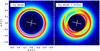 |
Fig. 5 Left: synthetic H-band image of the toy model presented in Sect. 5.2. Right: same model presented in the left panel, but adding an elliptical Gaussian artefact similar to that affecting our observations (see text for details). |
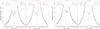 |
Fig. 6 Cuts along the disk major (left panel) and minor (right panel) axis. Each panel shows the cuts at H and K1-bands. Black asterisks and error bars represent the median and standard deviation at each position over a 3-px width slit along the major axis. A broken power-law profile is fitted at each side of the profile. The power-law indices are given in the legends of each panel, with the same color code as the fits plotted as solid curves, and correspond to the values listed in Table 1 (major axis) and Table 2 (minor axis). The vertical dotted line indicates the ~ 79 au cavity in the mm-sized grains (Zhang et al. 2014). The cuts are given in contrast (units of 10-4) with respect to the star at each band. |
As the disk is nearly face-on, we repeated the previous exercise but this time computed the profiles along the minor axis (due to projection effects, the difference between the minor and major axis remains below 0.5%). The southern side is brighter than the northern one (Fig. 6), as expected for an inclined disk with its nearest side on the southern direction (Fig. 5, left panel). This difference is higher (up to ~ 15%) at K1-band. As it happens with the major axis, we find that using a broken power-law produces a much more robust fit. The results from this fit are given in Table 2. We find again that the absolute value of the breaking point remains roughly constant for all the fits, and in excellent agreement with its counterpart along the major axis, with an average value of  (78.3 ± 1.5 au).
5.2.2. Azimuthal brightness profile
The azimuthal brightness profile was computed along the bright rim of the disk at H and K1-bands. The median and standard deviation were computed along the azimuthal direction using a 2-px width wedge with 5° opening angle (Fig. 7). The apparent local maxima around ~ 130° and ~−50° are aligned with the major axis of the elliptical artefact, thus they are probably a consequence of this artefact contamination. Excluding the artefact-dominated emission, the decrement in the dip with respect to the median of the −180°:−100° and 100°:180° regions is δK1 ~ 0.7 and δH ~ 0.6. The region between −60° and 100° (i.e., the northern side) shows lower brightness, as expected for an inclined disk with its nearest side on the south. We performed a non-linear, least squares Gaussian fit to the azimuthal profiles in the −30° to 70° range. The K1 fit produces a reduced Chi-squared of  with the center of the Gaussian located at 18.8° ± 0.7°. The H-band profile fit does not converge, most likely due to its higher contamination by artifacts.
 |
Fig. 7 Azimuthal profile at H and K1-bands, computed in a 2-px-width ring tracing the maximum of the ring at |

6. Discussion
As explained in the introduction, the radial structure of J1604 (both in dust and gas) matches several predictions by models of planet-disc interaction. Additionally, the accretion rate of J1604 is remarkably low (Ṁacc< 10-11M⊙ yr-1; EW (Hα) = 5.3 Å, Mathews et al. 2012a; van der Marel et al. 2016b) compared to the typical values found for most pre-transitional disks (median Ṁacc = 10-8.25M⊙yr-1, Kim et al. 2013). This is surprising considering the substantial amount of gas still present on the outer disk (Mgas = 0.02 M⊙van der Marel et al. 2015) despite the relative old age of the system (5–12 Myr).
The complex radial structure of the disk, and in particular the hot dust inside of the gas cavity, disagrees with photoevaporation or grain growth as potential mechanisms carving the disk (as already noted by Mathews et al. 2012b; Zhang et al. 2014; Pinilla et al. 2015). Dead-zones (poorly ionized disk regions, see e.g., Gammie 1996; Varnière & Tagger 2006; Regály et al. 2012) can create ring-like accumulations of large grains as a consequence of the change in viscosity at the outer edge of the dead-zone. However this mechanism does not create deep cavities in the gaseous distribution, and recent models predict a second ring composed by large grains also in the inner edge of the dead-zone (Ruge et al. 2016). Combining our results with the aperture-masking results by Kraus et al. (2008), stellar-mass companions are ruled out down to 2 au. In the most favorable case of an equal mass companion following an elliptical orbit with semi-major axis of 2 au, tidal truncation could at most open a ~ 5 au (in radius) cavity (Artymowicz & Lubow 1994) in the circumbinary disk. Therefore binarity cannot explain the radial structure of J1604. To summarise, the structure of J1604 most likely reflects interactions between the disk and sub-stellar companion(s).
According to the BT-Settl models (hot start scenario), our observations are sensitive to planets with masses exceeding ≳2.5 MJup across the disk cavity, except in the 14.5–22 au range where the sensitivity drops to ≳9–4 MJup (Fig. 3). The warm start scenario is less stringent, and predicts that planets below ~ 6 MJup will escape detection. Some studies associate the hot- and warm- start scenarios to planet formation via gravitational instability and core accretion, respectively. However, Mordasini (2013) show that care must be taken with this classification as planets formed via core accretion may have similar properties to those formed via a hot start scenario.
6.1. Multiple Jovian planets?
Planets and disk properties can be related by the widths and depths of planetary gaps produced by numerical simulations. The size of the cavity carved by a planet depends on the planet orbit (rp) and the Hill radius rH = rp(q/ 3)1/3, where q is the planet/star mass ratio. de Juan Ovelar et al. (2016) show that large cavities carved by planets in the mm- and μm -sized grain populations most likely indicate a turbulent mixing (directly related to the disk viscosity) of αturb ~ 10-3. In what follows, we adopt this value for comparison with model predictions. Following Pinilla et al. (2012), one massive (≥5 MJup) giant planet will open a gap of ~ 5rH in the gas and ~ 10rH in the dust, that is, the dust cavity can be up to twice the size of the gas cavity. Dong et al. (2015b) analyzes the effect of multiple planets, finding that multiple low-mass planets (e.g., 3 × 0.2 MJup) cannot open a large dust gap/cavity as they will just clear up narrow gaps. Regarding the depth of the cavity, planets reduce the amount of gas inside of the cavities, with more massive planets creating more gas-depleted cavities. For instance, one 9 MJup planet should deplete the gas surface density by a factor ~ 10-3, which is roughly two orders of magnitude higher than what is observed for J1604 (δco ~ 10-5, van der Marel et al. 2015). On the other hand, Duffell & Dong (2015) show that, in general, gas cavities created by multiple planets are shallower (i.e., less gas depleted) than those created by one single planet. Finally, planets can also reduce the accretion rates onto their host star (e.g., Alexander & Armitage 2007), and Zhu et al. (2011) show that for a standard disk accreting at Ṁacc ~ 10-8M⊙ yr-1, multiple planets are needed to reduce the accretion rate below Ṁacc = 10-9M⊙ yr-1 (see also Espaillat et al. 2014).
Combining all the previous predictions, one configuration in agreement with our observations and current theories of planet-disk interaction could be the following: a ~ 15 MJup brown dwarf orbiting at ~ 15 au (or more massive at closer orbits) would remain undetected, while it could account for the ~ 30 au, δco ~ 10-5 gas depleted cavity (Pinilla et al. 2012; Fung et al. 2014). One or more Jovian planets at larger orbits could then explain the very low accretion rate and larger dust cavities, while creating very narrow and shallow gaps in the gas that would remain undetected with the sensitivity and spatial resolution of current ALMA observations. Of course, the scenario we just described is only one possibility. In general, and despite our deep observations, this problem is degenerated, which prevents us from deriving further constraints on the orbits and masses of this hypothetical multi-planetary system.
6.2. Disk surface
The radial brightness profiles along the major and minor axes (Figs. 6 and 7) show that the dust in the disk surface scatters slightly more light towards longer wavelengths. We note that these profiles are given in contrast units for each band, such that the variation of stellar flux with wavelength is automatically considered. Taking into account that the H-band image is more contaminated by the elliptical artefact (i.e., receives more flux from it) than the K1 image, then the brightness profiles indicate that the disk has a red color. Scattering in the Rayleigh regime (2πa<λ) produces very blue colours (as the scattering efficiency in this regime scales with λ-4). Therefore, our images indicate that the population of grains on the disk surface is dominated by grains with an average size ≳0.3 μm (see e.g., Mulders et al. 2013, for a discussion on dust properties derived from scattered light images at NIR). The artefact contamination makes it difficult to obtain a more detailed description of the dust properties. Imaging polarimetry observations of other planet-forming candidate disks also reveal broken-power law brightness profiles (HD 169142, HD 135344B, Quanz et al. 2013b; Garufi et al. 2013) and red disk colours (HD 100546, HD 142527, Mulders et al. 2013; Canovas et al. 2013; Avenhaus et al. 2014).
There are different estimates for the power-law index of the radial profile in the literature, all derived from polarized intensity observations. Pinilla et al. (2015) computes the azimuthally averaged radial profile at R-band, obtaining a power-law index of α = −2.92 ± 0.03. Mayama et al. (2012) follow a different approach and fit a power-law along the major axis using a 30° width slit centered at 80° east of north, obtaining α = −4.7 ± 0.1 and α = −4.0 ± 0.2 for the eastern and western sides, respectively. While these values are different from those presented here, we note that they were computed over a much larger azimuthal range than our values listed in Table 1, which were computed using a narrow 3-px width slit centered on the most recent value derived for the position angle (PA ~ 77°). The brightness profiles of our images become more steep (with power-law index >−3, see Whitney & Hartmann 1992) at ~ 79 au, which coincides with the cavity size for the large grains derived by Zhang et al. (2014). Inwards of that radius, our profiles become more flat (power-law index <−3). This suggests that the surface of the disk, where the small grains are located, is sensitive to the change in the radial distribution of the large grains, which are mostly concentrated around the disk’s cold midplane.
The observations presented by Pinilla et al. (2015) were recorded one night later than the data set we present here. They fit the dip with a Gaussian profile and derive a position angle of 46.2° ± 5.4° east of north, and a depletion factor δdip ~ 0.72. The relatively large difference between their derived position angle and ours (~ 18.8° ± 0.6° at K1) is probably best explained by the much lower S/N of their images. Following Pinilla et al. (2015), assuming that the dip observed by Mayama et al. (2012) is the same feature observed here, then it rotates at ~ 22° yr-1 (e.g., period of ~ 16.4 yr, roughly half the period previously derived). The dip could be a shadow casted by an inner body/dust structure, located at a Keplerian orbit with a ~ 6.3 au radius. We note that a tilted inner disk should produce either two sharp shadows or an azimuthally large, smooth, single shadow (Marino et al. 2015; Stolker et al. 2016). On the other hand, a point source, or a very flat structure, cannot cast a shadow on the disk surface, as this shadow would be cast around the disk midplane only. We hypothesize that a low-mass companion surrounded by a disk orbiting at ~ 6 au, with a disk diameter of ~ 3 au and scale height ~ 0.8 au could cast a shadow over the disk surface. This would create a dip in brightness with similar morphology to what is observed in J1604.
7. Summary
We present deep, high-contrast SPHERE/VLT observations of the pre-transitional disk J1604. This disk shows several features that suggest planet-disk interactions, such as different cavity sizes in its gas and dust distributions. Despite reaching a contrast of ~ Δ12 mag at YJH and K-bands from  , we do not detect any point source. Translating our limits to mass sensitivity, and assuming a distance of 145 pc and an age ranging from 5 to 12 Myr, we are sensitive to planets with masses ≳2.5 MJup if formed via a hot start scenario at 22 to 115 au from the star. Alternatively, we are sensitive to ≳6 MJup in the same distance range if the planets formed via a warm start scenario. Combining our non-detection with the observed cavity sizes and accretion rates of J1604, and comparing these observational constraints with the predictions of models describing planet-disk interactions, we conclude that J1604 is most likely a multi-planetary system.
We find that the decrement in the disk bright inner rim is located at ~ 18.8° at K1-band. This dip could be produced by a large structure in Keplerian motion around the central star. A consistent speculative scenario would thus be a brown dwarf (up to 20 MJup given the detection limits from Kraus et al. 2008) surrounded by an accretion disk at 6 au from the central object. Such a brown dwarf+disk system could have the Keplerian velocity and extension needed to explain the moving shadow and would still escape a detection. Additional Jovian planets at larger radii could account for the observed properties of J1604 while explaining our non-detection. The expected details of our proposed multiple system configuration are yet to be explored by models.
Our observations reveal, for the first time, the disk around J1604 in scattered light at all Y,J,H,K-bands. Despite being affected by artefacts, we show that the disk color is red, which is best explained by dust particles with an average size ≳0.3 μm. We find that the brightness radial profile changes its slope at ~ 79 au, which matches the cavity size radius for the mm-sized particles derived by Zhang et al. (2014). This suggests that there is a relationship between the change in the flaring angle of the disk (traced by the scattered light images sensitive to the small dust grains in the disk surface), and the radial distribution of the large grains in the disk midplane.
Overall, J1604 shows very different properties than the majority of well-known transitional (and pre-transitional) disks. Its extremely low accretion rate (Ṁacc< 10-11M⊙ yr-1, Mathews et al. 2012a) seems to be in contradiction with the large amount of gas mass (Mgas ~ 0.02 M⊙, van der Marel et al. 2015) still present in this 5–12 Myr old disk. The gas cavity is the most gas-depleted cavity in the sample studied by van der Marel et al. (2015) and van der Marel et al. (2016a). Finally we note that, although multiple planets are currently the most realistic explanation, photoevaporation and other mechanisms (e.g., a dead-zone) could also be creating the observed features.
The fluxes from Spiegel & Burrows (2012) were converted to the SPHERE photometric system using the filter transmission curves given in https://www.eso.org/sci/facilities/paranal/instruments/sphere/inst/filters.html
Acknowledgments
We thank the referee for his/her useful comments. H.C., E.V., and G.M. acknowledges support from the Spanish Ministerio de Economía y Competitividad under grant AYA 2014-55840-P. G.M. is funded by the Spanish grant RyC-2011-07920. This research was partially funded by the Millennium Science Initiative, Chilean Ministry of Economy, Nucleus RC130007. C.C. acknowledges support from CONICYT PAI/Concurso nacional de inserción en la academia, convocatoria 2015, Folio 79150049, and CONICYT-FONDECYT grant 3140592. M.R.S. acknowledge support from FONDECYT grant 1141269. L.C. was supported by ALMA-CONICYT and CONICYT-FONDECYT 31120009 and 1140109.
References
- Alexander, R. D., & Armitage, P. J. 2007, MNRAS, 375, 500 [NASA ADS] [CrossRef] [Google Scholar]
- Allard, F., Homeier, D., & Freytag, B. 2011, in 16th Cambridge Workshop on Cool Stars, Stellar Systems, and the Sun, eds. C. Johns-Krull, M. K. Browning, & A. A. West, ASP Conf. Ser., 448, 91 [Google Scholar]
- Allard, F., Homeier, D., Freytag, B., et al. 2013, Mem. Soc. Astron. It. Suppl., 24, 128 [Google Scholar]
- Andrews, S. M., Wilner, D. J., Espaillat, C., et al. 2011, ApJ, 732, 42 [NASA ADS] [CrossRef] [Google Scholar]
- Artymowicz, P., & Lubow, S. H. 1994, ApJ, 421, 651 [NASA ADS] [CrossRef] [Google Scholar]
- Avenhaus, H., Quanz, S. P., Schmid, H. M., et al. 2014, ApJ, 781, 87 [NASA ADS] [CrossRef] [Google Scholar]
- Baraffe, I., Homeier, D., Allard, F., & Chabrier, G. 2015, A&A, 577, A42 [NASA ADS] [CrossRef] [EDP Sciences] [Google Scholar]
- Beuzit, J.-L., Feldt, M., Dohlen, K., et al. 2008, in SPIE Conf. Ser., 7014, 18 [Google Scholar]
- Biller, B. A., Males, J., Rodigas, T., et al. 2014, ApJ, 792, L22 [NASA ADS] [CrossRef] [Google Scholar]
- Boss, A. P. 1997, Science, 276, 1836 [NASA ADS] [CrossRef] [Google Scholar]
- Boss, A. P., Butler, R. P., Hubbard, W. B., et al. 2007, Trans. IAU, Ser. A, 26, 183 [Google Scholar]
- Caceres, C., Hardy, A., Schreiber, M. R., et al. 2015, ApJ, 806, L22 [NASA ADS] [CrossRef] [Google Scholar]
- Canovas, H., Ménard, F., Hales, A., et al. 2013, A&A, 556, A123 [NASA ADS] [CrossRef] [EDP Sciences] [Google Scholar]
- Canovas, H., Schreiber, M. R., Cáceres, C., et al. 2015, ApJ, 805, 21 [NASA ADS] [CrossRef] [Google Scholar]
- Canovas, H., Caceres, C., Schreiber, M. R., et al. 2016, MNRAS, 458, L29 [NASA ADS] [CrossRef] [Google Scholar]
- Carbillet, M., Bendjoya, P., Abe, L., et al. 2011, Exp. Astron., 30, 39 [NASA ADS] [CrossRef] [Google Scholar]
- Carpenter, J. M., Mamajek, E. E., Hillenbrand, L. A., & Meyer, M. R. 2006, ApJ, 651, L49 [NASA ADS] [CrossRef] [Google Scholar]
- Carpenter, J. M., Mamajek, E. E., Hillenbrand, L. A., & Meyer, M. R. 2009, ApJ, 705, 1646 [Google Scholar]
- Carpenter, J. M., Ricci, L., & Isella, A. 2014, ApJ, 787, 42 [NASA ADS] [CrossRef] [Google Scholar]
- Casassus, S., van der Plas, G., Perez, S. M., et al. 2013, Nature, 493, 191 [NASA ADS] [CrossRef] [Google Scholar]
- Cieza, L. A., Mathews, G. S., Williams, J. P., et al. 2012, ApJ, 752, 75 [NASA ADS] [CrossRef] [Google Scholar]
- Claudi, R. U., Turatto, M., Gratton, R. G., et al. 2008, in SPIE Conf. Ser., 7014, 3 [Google Scholar]
- Currie, T., Muto, T., Kudo, T., et al. 2014, ApJ, 796, L30 [NASA ADS] [CrossRef] [Google Scholar]
- Currie, T., Cloutier, R., Brittain, S., et al. 2015, ApJ, 814, L27 [NASA ADS] [CrossRef] [Google Scholar]
- Dahm, S. E., & Carpenter, J. M. 2009, AJ, 137, 4024 [NASA ADS] [CrossRef] [Google Scholar]
- de Geus, E. J., de Zeeuw, P. T., & Lub, J. 1989, A&A, 216, 44 [NASA ADS] [Google Scholar]
- de Juan Ovelar, M., Pinilla, P., Min, M., Dominik, C., & Birnstiel, T. 2016, MNRAS, 459, L85 [NASA ADS] [CrossRef] [Google Scholar]
- de Zeeuw, P. T., Hoogerwerf, R., de Bruijne, J. H. J., Brown, A. G. A., & Blaauw, A. 1999, AJ, 117, 354 [NASA ADS] [CrossRef] [Google Scholar]
- Dohlen, K., Langlois, M., Saisse, M., et al. 2008, in SPIE Conf. Ser., 7014, 3 [Google Scholar]
- Dong, R., Zhu, Z., Rafikov, R. R., & Stone, J. M. 2015a, ApJ, 809, L5 [NASA ADS] [CrossRef] [Google Scholar]
- Dong, R., Zhu, Z., & Whitney, B. 2015b, ApJ, 809, 93 [NASA ADS] [CrossRef] [Google Scholar]
- Dong, R., Zhu, Z., Fung, J., et al. 2016, ApJ, 816, L12 [NASA ADS] [CrossRef] [Google Scholar]
- Draine, B. T. 2003, ARA&A, 41, 241 [NASA ADS] [CrossRef] [Google Scholar]
- Draine, B. T., & Lee, H. M. 1984, ApJ, 285, 89 [Google Scholar]
- Duffell, P. C., & Dong, R. 2015, ApJ, 802, 42 [NASA ADS] [CrossRef] [Google Scholar]
- Espaillat, C., Calvet, N., D’Alessio, P., et al. 2007, ApJ, 670, L135 [NASA ADS] [CrossRef] [Google Scholar]
- Espaillat, C., Muzerolle, J., Najita, J., et al. 2014, Protostars and Planets VI, 497 [Google Scholar]
- Fung, J., Shi, J.-M., & Chiang, E. 2014, ApJ, 782, 88 [NASA ADS] [CrossRef] [Google Scholar]
- Gammie, C. F. 1996, ApJ, 457, 355 [NASA ADS] [CrossRef] [Google Scholar]
- Garufi, A., Quanz, S. P., Avenhaus, H., et al. 2013, A&A, 560, A105 [NASA ADS] [CrossRef] [EDP Sciences] [Google Scholar]
- Huélamo, N., Lacour, S., Tuthill, P., et al. 2011, A&A, 528, L7 [NASA ADS] [CrossRef] [EDP Sciences] [Google Scholar]
- Hughes, A. M., Andrews, S. M., Espaillat, C., et al. 2009, ApJ, 698, 131 [NASA ADS] [CrossRef] [Google Scholar]
- Ireland, M. J., Kraus, A., Martinache, F., Law, N., & Hillenbrand, L. A. 2011, ApJ, 726, 113 [NASA ADS] [CrossRef] [Google Scholar]
- Juhász, A., Benisty, M., Pohl, A., et al. 2015, MNRAS, 451, 1147 [NASA ADS] [CrossRef] [Google Scholar]
- Kim, K. H., Watson, D. M., Manoj, P., et al. 2013, ApJ, 769, 149 [NASA ADS] [CrossRef] [Google Scholar]
- Kraus, A. L., & Hillenbrand, L. A. 2009, ApJ, 703, 1511 [NASA ADS] [CrossRef] [Google Scholar]
- Kraus, A. L., & Ireland, M. J. 2012, ApJ, 745, 5 [NASA ADS] [CrossRef] [Google Scholar]
- Kraus, A. L., Ireland, M. J., Martinache, F., & Lloyd, J. P. 2008, ApJ, 679, 762 [NASA ADS] [CrossRef] [Google Scholar]
- Kraus, A. L., Ireland, M. J., Cieza, L. A., et al. 2014, ApJ, 781, 20 [NASA ADS] [CrossRef] [Google Scholar]
- Lafrenière, D., Marois, C., Doyon, R., Nadeau, D., & Artigau, É. 2007, ApJ, 660, 770 [NASA ADS] [CrossRef] [Google Scholar]
- Lubow, S. H., Seibert, M., & Artymowicz, P. 1999, ApJ, 526, 1001 [NASA ADS] [CrossRef] [Google Scholar]
- Maire, A.-L., Bonnefoy, M., Ginski, C., et al. 2016, A&A, 587, A56 [NASA ADS] [CrossRef] [EDP Sciences] [Google Scholar]
- Marino, S., Perez, S., & Casassus, S. 2015, ApJ, 798, L44 [NASA ADS] [CrossRef] [Google Scholar]
- Marois, C., Lafrenière, D., Doyon, R., Macintosh, B., & Nadeau, D. 2006, ApJ, 641, 556 [Google Scholar]
- Mathews, G. S., Williams, J. P., & Ménard, F. 2012a, ApJ, 753, 59 [NASA ADS] [CrossRef] [Google Scholar]
- Mathews, G. S., Williams, J. P., Ménard, F., et al. 2012b, ApJ, 745, 23 [NASA ADS] [CrossRef] [Google Scholar]
- Mathews, G. S., Pinte, C., Duchêne, G., Williams, J. P., & Ménard, F. 2013, A&A, 558, A66 [NASA ADS] [CrossRef] [EDP Sciences] [Google Scholar]
- Mawet, D., Milli, J., Wahhaj, Z., et al. 2014, ApJ, 792, 97 [NASA ADS] [CrossRef] [Google Scholar]
- Mayama, S., Hashimoto, J., Muto, T., et al. 2012, ApJ, 760, L26 [NASA ADS] [CrossRef] [Google Scholar]
- Mesa, D., Gratton, R., Zurlo, A., et al. 2015, A&A, 576, A121 [NASA ADS] [CrossRef] [EDP Sciences] [Google Scholar]
- Mie, G. 1908, Ann. Phys. Leipzig, 330, 377 [NASA ADS] [CrossRef] [Google Scholar]
- Min, M., Hovenier, J. W., & de Koter, A. 2005, A&A, 432, 909 [NASA ADS] [CrossRef] [EDP Sciences] [Google Scholar]
- Mordasini, C. 2013, A&A, 558, A113 [NASA ADS] [CrossRef] [EDP Sciences] [Google Scholar]
- Mulders, G. D., Min, M., Dominik, C., Debes, J. H., & Schneider, G. 2013, A&A, 549, A112 [NASA ADS] [CrossRef] [EDP Sciences] [Google Scholar]
- Olofsson, J., Benisty, M., Le Bouquin, J.-B., et al. 2013, A&A, 552, A4 [NASA ADS] [CrossRef] [EDP Sciences] [Google Scholar]
- Paardekooper, S.-J., & Mellema, G. 2006, A&A, 453, 1129 [NASA ADS] [CrossRef] [EDP Sciences] [Google Scholar]
- Pavlov, A., Möller-Nilsson, O., Feldt, M., et al. 2008, in SPIE Conf. Ser., 7019, 701939 [Google Scholar]
- Pecaut, M. J., Mamajek, E. E., & Bubar, E. J. 2012, ApJ, 746, 154 [NASA ADS] [CrossRef] [Google Scholar]
- Pinilla, P., Benisty, M., & Birnstiel, T. 2012, A&A, 545, A81 [NASA ADS] [CrossRef] [EDP Sciences] [Google Scholar]
- Pinilla, P., de Boer, J., Benisty, M., et al. 2015, A&A, 584, L4 [NASA ADS] [CrossRef] [EDP Sciences] [Google Scholar]
- Pinte, C., Ménard, F., Duchêne, G., & Bastien, P. 2006, A&A, 459, 797 [NASA ADS] [CrossRef] [EDP Sciences] [Google Scholar]
- Pinte, C., Harries, T. J., Min, M., et al. 2009, A&A, 498, 967 [NASA ADS] [CrossRef] [EDP Sciences] [Google Scholar]
- Pollack, J. B., Hubickyj, O., Bodenheimer, P., et al. 1996, Icarus, 124, 62 [NASA ADS] [CrossRef] [Google Scholar]
- Preibisch, T., Brown, A. G. A., Bridges, T., Guenther, E., & Zinnecker, H. 2002, AJ, 124, 404 [NASA ADS] [CrossRef] [Google Scholar]
- Pueyo, L., Soummer, R., Hoffmann, J., et al. 2015, ApJ, 803, 31 [NASA ADS] [CrossRef] [Google Scholar]
- Quanz, S. P., Amara, A., Meyer, M. R., et al. 2013a, ApJ, 766, L1 [NASA ADS] [CrossRef] [Google Scholar]
- Quanz, S. P., Avenhaus, H., Buenzli, E., et al. 2013b, ApJ, 766, L2 [NASA ADS] [CrossRef] [Google Scholar]
- Quanz, S. P., Amara, A., Meyer, M. R., et al. 2015, ApJ, 807, 64 [NASA ADS] [CrossRef] [Google Scholar]
- Racine, R., Walker, G. A. H., Nadeau, D., Doyon, R., & Marois, C. 1999, PASP, 111, 587 [NASA ADS] [CrossRef] [Google Scholar]
- Rafikov, R. R. 2011, ApJ, 727, 86 [NASA ADS] [CrossRef] [Google Scholar]
- Regály, Z., Juhász, A., Sándor, Z., & Dullemond, C. P. 2012, MNRAS, 419, 1701 [NASA ADS] [CrossRef] [Google Scholar]
- Reggiani, M., Quanz, S. P., Meyer, M. R., et al. 2014, ApJ, 792, L23 [NASA ADS] [CrossRef] [Google Scholar]
- Rice, W. K. M., Armitage, P. J., Wood, K., & Lodato, G. 2006, MNRAS, 373, 1619 [NASA ADS] [CrossRef] [Google Scholar]
- Ruge, J. P., Flock, M., Wolf, S., et al. 2016, A&A, 590, A17 [NASA ADS] [CrossRef] [EDP Sciences] [Google Scholar]
- Sallum, S., Follette, K. B., Eisner, J. A., et al. 2015, Nature, 527, 342 [NASA ADS] [CrossRef] [Google Scholar]
- Soummer, R. 2005, ApJ, 618, L161 [NASA ADS] [CrossRef] [Google Scholar]
- Soummer, R., Pueyo, L., & Larkin, J. 2012, ApJ, 755, L28 [NASA ADS] [CrossRef] [Google Scholar]
- Spiegel, D. S., & Burrows, A. 2012, ApJ, 745, 174 [NASA ADS] [CrossRef] [Google Scholar]
- Stolker, T., Dominik, C., Avenhaus, H., et al. 2016, A&A, 595, A113 [NASA ADS] [CrossRef] [EDP Sciences] [Google Scholar]
- Strom, K. M., Strom, S. E., Edwards, S., Cabrit, S., & Skrutskie, M. F. 1989, AJ, 97, 1451 [NASA ADS] [CrossRef] [Google Scholar]
- van der Marel, N., van Dishoeck, E. F., Bruderer, S., Pérez, L., & Isella, A. 2015, A&A, 579, A106 [NASA ADS] [CrossRef] [EDP Sciences] [Google Scholar]
- van der Marel, N., van Dishoeck, E. F., Bruderer, S., et al. 2016a, A&A, 585, A58 [NASA ADS] [CrossRef] [EDP Sciences] [Google Scholar]
- van der Marel, N., Verhaar, B. W., van Terwisga, S., et al. 2016b, A&A, 592, A126 [NASA ADS] [CrossRef] [EDP Sciences] [Google Scholar]
- Varnière, P., & Tagger, M. 2006, A&A, 446, L13 [NASA ADS] [CrossRef] [EDP Sciences] [Google Scholar]
- Vigan, A., Moutou, C., Langlois, M., et al. 2010, MNRAS, 407, 71 [NASA ADS] [CrossRef] [Google Scholar]
- Vigan, A., Gry, C., Salter, G., et al. 2015, MNRAS, 454, 129 [NASA ADS] [CrossRef] [Google Scholar]
- Vigan, A., Bonnefoy, M., Ginski, C., et al. 2016, A&A, 587, A55 [NASA ADS] [CrossRef] [EDP Sciences] [Google Scholar]
- Wahhaj, Z., Cieza, L. A., Mawet, D., et al. 2015, A&A, 581, A24 [NASA ADS] [CrossRef] [EDP Sciences] [Google Scholar]
- Whitney, B. A., & Hartmann, L. 1992, ApJ, 395, 529 [NASA ADS] [CrossRef] [Google Scholar]
- Winn, J. N., & Fabrycky, D. C. 2015, ARA&A, 53, 409 [NASA ADS] [CrossRef] [Google Scholar]
- Zhang, K., Isella, A., Carpenter, J. M., & Blake, G. A. 2014, ApJ, 791, 42 [NASA ADS] [CrossRef] [Google Scholar]
- Zhu, Z., Nelson, R. P., Hartmann, L., Espaillat, C., & Calvet, N. 2011, ApJ, 729, 47 [NASA ADS] [CrossRef] [Google Scholar]
- Zurlo, A., Vigan, A., Mesa, D., et al. 2014, A&A, 572, A85 [NASA ADS] [CrossRef] [EDP Sciences] [Google Scholar]
- Zurlo, A., Vigan, A., Galicher, R., et al. 2016, A&A, 587, A57 [NASA ADS] [CrossRef] [EDP Sciences] [Google Scholar]
All Tables
All Figures
|
Fig. 1 PCA reduced image of the IRDIS K1 filter. The image has a software mask of radii |
| In the text | |
|
Fig. 2 Azimuthally averaged contrast curves (5σ detection limits) derived using the methods described in Sect. 5.1. The black solid line traces the contrast of the averaged off-axis PSF at K1-band. The vertical dotted line indicates the IWA of our images. The dashed line indicates the detection limits derived by Kraus et al. (2008). |
| In the text | |
|
Fig. 3 Physical limits on planetary mass companions derived as described in Sect. 5.1. The IFS mass limits are slightly better than the IRDIS ones. The shadowed area reflects the large uncertainty on the age of the plausible companions, ranging from 5 to 12 Myr. There are no warm start models for planets with masses above 10 MJup. The “hump” in sensitivity at ~ 60 au is due to disk emission. Mass limits from 115 to 130 au correspond to IRDIS K1-band observations using the same methodology as for the IFS. |
| In the text | |
|
Fig. 4 Scattered light images of the disk (Sect. 3.4) at different bands after applying an unsharp filter as described in Sect. 5.2. A software mask of radius |
| In the text | |
|
Fig. 5 Left: synthetic H-band image of the toy model presented in Sect. 5.2. Right: same model presented in the left panel, but adding an elliptical Gaussian artefact similar to that affecting our observations (see text for details). |
| In the text | |
|
Fig. 6 Cuts along the disk major (left panel) and minor (right panel) axis. Each panel shows the cuts at H and K1-bands. Black asterisks and error bars represent the median and standard deviation at each position over a 3-px width slit along the major axis. A broken power-law profile is fitted at each side of the profile. The power-law indices are given in the legends of each panel, with the same color code as the fits plotted as solid curves, and correspond to the values listed in Table 1 (major axis) and Table 2 (minor axis). The vertical dotted line indicates the ~ 79 au cavity in the mm-sized grains (Zhang et al. 2014). The cuts are given in contrast (units of 10-4) with respect to the star at each band. |
| In the text | |
|
Fig. 7 Azimuthal profile at H and K1-bands, computed in a 2-px-width ring tracing the maximum of the ring at |
| In the text | |
Current usage metrics show cumulative count of Article Views (full-text article views including HTML views, PDF and ePub downloads, according to the available data) and Abstracts Views on Vision4Press platform.
Data correspond to usage on the plateform after 2015. The current usage metrics is available 48-96 hours after online publication and is updated daily on week days.
Initial download of the metrics may take a while.