| Issue |
A&A
Volume 598, February 2017
|
|
|---|---|---|
| Article Number | A1 | |
| Number of page(s) | 23 | |
| Section | Extragalactic astronomy | |
| DOI | https://doi.org/10.1051/0004-6361/201527969 | |
| Published online | 24 January 2017 | |
[Ultra] luminous infrared galaxies selected at 90 μm in the AKARI deep field: a study of AGN types contributing to their infrared emission⋆
1 National Centre for Nuclear Research, ul. Hoża 69, 00-681 Warszawa, Poland
e-mail: This email address is being protected from spambots. You need JavaScript enabled to view it.
2 The Astronomical Observatory of the Jagiellonian University, ul. Orla 171, 30-244 Kraków, Poland
3 Laboratoire d’Astrophysique de Marseille, OAMP, Université Aix-Marseille, CNRS, 38 rue Frédéric Joliot-Curie, 13388 Marseille Cedex 13, France
4 Department of Particle and Astrophysical Science, Nagoya University, Furo-cho, Chikusa-ku, 464-8602 Nagoya, Japan
5 Dark Cosmology Centre, Niels Bohr Institute, University of Copenhagen, Juliane Maries Vej 30, 2100 Copenhagen, Denmark
6 Department of Physics and Astronomy, University of California, Los Angeles, CA 90024, USA
7 Institute of Space and Astronautical Science, Japan Aerospace Exploration Agency, Sagamihara, 229-8510 Kanagawa, Japan
Received: 15 December 2015
Accepted: 16 November 2016
Abstract
Aims. The aim of this work is to characterize physical properties of ultra luminous infrared galaxies (ULIRGs) and luminous infrared galaxies (LIRGs) detected in the far-infrared (FIR) 90 μm band in the AKARI Deep Field-South (ADF-S) survey. In particular, we want to estimate the active galactic nucleus (AGN) contribution to the LIRGs and ULIRGs’ infrared emission and which types of AGNs are related to their activity.
Methods. We examined 69 galaxies at redshift ≥0.05 detected at 90 μm by the AKARI satellite in the ADF-S, with optical counterparts and spectral coverage from the ultraviolet to the FIR. We used two independent spectral energy distribution fitting codes: one fitting the SED from FIR to FUV (CIGALE) (we use the results from CIGALE as a reference) and gray-body + power spectrum fit for the infrared part of the spectra (CMCIRSED) in order to identify a subsample of ULIRGs and LIRGs, and to estimate their properties.
Results. Based on the CIGALE SED fitting, we have found that LIRGs and ULIRGs selected at the 90 μm AKARI band compose ~56% of our sample (we found 17 ULIRGs and 22 LIRGs, spanning over the redshift range 0.06 <z< 1.23). Their physical parameters, such as stellar mass, star formation rate (SFR), and specific SFR are consistent with the ones found for other samples selected at infrared wavelengths. We have detected a significant AGN contribution to the mid-infrared luminosity for 63% of LIRGs and ULIRGs. Our LIRGs contain Type 1, Type 2, and intermediate types of AGN, whereas for ULIRGs, a majority (more than 50%) of AGN emission originates from Type 2 AGNs. The temperature-luminosity and temperature-mass relations for the dust component of ADF–S LIRGs and ULIRGs indicate that these relations are shaped by the dust mass and not by the increased dust heating.
Conclusions. We conclude that LIRGs contain Type 1, Type 2, and intermediate types of AGNs, with an AGN contribution to the mid infrared emission at the median level of 13 ± 3%, whereas the majority of ULIRGs contain Type 2 AGNs, with a median AGN fraction equal to 19 ± 8%.
Key words: galaxies: active / infrared: galaxies / galaxies: statistics / galaxies: Seyfert
Full Table A.1 is only available at the CDS via anonymous ftp to cdsarc.u-strasbg.fr (130.79.128.5) or via http://cdsarc.u-strasbg.fr/viz-bin/qcat?J/A+A/598/A1
© ESO, 2017
1. Introduction
The first infrared all-sky survey performed by the satellite The Infra-Red Astronomical Satellite (IRAS, Soifer et al. 1987; Neugebauer et al. 1984) in the early 1980s established the existence of galaxies emitting very brightly in infrared (IR) wavelengths with total IR luminosities greater than 1012 [L⊙]. These were thus named ultra luminous infrared galaxies (ULIRGs; e.g., Houck et al. 1985; Soifer et al. 1986). Sanders et al. (1988) reported a discovery of ten infrared objects with luminosities ![Mathematical equation: \hbox{$L_{(8-1000~\mu {\rm m})} \geqslant 10^{12}~[L_{\odot}]$}](/articles/aa/full_html/2017/02/aa27969-15/aa27969-15-eq9.png) in the IRAS Bright Galaxy Sample. Analysis of this first sample of ULIRGs has shown that these sources are often interacting galaxies, and in the near-infrared colors they appear to be a mixture of starburst and active galactic nuclei (AGN).
in the IRAS Bright Galaxy Sample. Analysis of this first sample of ULIRGs has shown that these sources are often interacting galaxies, and in the near-infrared colors they appear to be a mixture of starburst and active galactic nuclei (AGN).
The properties of this sample of galaxies have been the subject of numerous analyses. Many physical properties, such as the dust temperature, the star formation rate (SFR), and the mass-luminosity relationship were derived based on the local examples of ULIRG samples, but their global evolution remains unclear (Lonsdale et al. 2006). Previous studies indicate that in the local Universe ULIRGs are rather rare objects (Kim & Sanders 1998), but at higher redshift they become more common (Takeuchi et al. 2005; Symeonidis et al. 2011, 2013). A group of sources, ten times fainter in the IR, known as luminous infrared galaxies (LIRGs) and characterized by a total IR luminosity between 1011 and 1012 [L⊙], Soifer et al. 1986), is very often analyzed together with ULIRGs.
There is no straightforward explanation of the nature of LIRGs and ULIRGs. It appears that the majority of local ULIRGs are merger systems of gas-reach disk galaxies (Murphy et al. 1996; Clements et al. 1996; Veilleux et al. 2002; Lonsdale et al. 2006), whereas local LIRGs have more varied morphologies (Hung et al. 2014); they emit most of their energy (over 90%) in the IR, which implies that they are heavily obscured by dust (Sanders & Mirabel 1996). Despite a very luminous dust component, LIRGs and ULIRGs have moderate luminosities in optical bands. For this reason, to explain their very high IR luminosities, these objects must have ongoing, extreme star-formation processes, forming new stars at rates of an order of 100 M⊙ yr-1 (based on the Kennicutt 1998 equation; and results published by e.g., Noeske et al. 2007; da Cunha et al. 2010, 2015; Howell et al. 2010; Podigachoski et al. 2015). This very violent star formation is almost undetectable at wavelengths different from IR.
As demonstrated by previous studies, on average, more than 25% (Veilleux et al. 1997), 30% (Clements et al. 1996; U et al. 2012), 40% (Farrah et al. 2007), 50% (Alonso-Herrero et al. 2012; Carpineti et al. 2015), and 70% (Nardini et al. 2010) of local LIRGs and ULIRGs host an AGN. Veilleux et al. (2009) found that all local ULIRGs have some AGN contribution to the bolometric luminosity. Based on the results presented above it is possible to conclude that the percentage of LIRGs and ULIRGs hosting an AGN depends on the sample selection and the diagnostic method used to identify the AGN. Previous studies have also shown that the relative contribution of AGNs to the bolometric luminosities is only a few percent (from 7 to 10%) of the total luminosity of local LIRGs (Pereira-Santaella et al. 2011; Petric et al. 2011), and ~20% of local ULIRGs (Farrah et al. 2007; Nardini et al. 2009). Consequently, the most likely dominant contributor to the total IR emission in most ULIRGs is star formation. Veilleux et al. (2009), based on the IRAS 1 Jy sample, found that the AGN contribution to local ULIRGs may range from 7% to even 95% with an average contribution of 35−40%, and that this value strongly depends on the dust luminosity. Lee et al. (2011) show that ULIRGs more often host Type 2 AGNs than Type 1 (hereafter: Type 2 ULIRGs, and Type 1 ULIRGs), and the percentage of Type 2 ULIRGs increases with infrared luminosity. Their sample of 115 ULIRGs includes only eight broad-line AGNs, and 49 narrow-line AGNs (activity of 58 was found to be non-AGN–related). Kim (1995) came to a similar conclusion. Analogous results were presented by Veilleux et al. (2009) (12 Type 2 ULIRGs and 9 Type 1 ULIRGs), but in this case the difference is insignificant. The fact that these findings were based on almost the same selection of objects (IRAS 1 Jy and Spitzer 1 Jy surveys) poses the question as to whether or not ULIRGs selected in a different way have similar properties.
Previous studies (Chary & Elbaz 2001; Le Floc’h et al. 2005; Pérez-González et al. 2005; Magnelli et al. 2009; Goto et al. 2010) show that galaxies with total IR luminosity > 1011 [L⊙] are the major contributors to the star-formation density at redshifts of ~1−2. The co-moving number density of LIRGs from the Magnelli et al. (2009) sample has increased by a factor of approximately 100 between z ~ 0 and z ~ 1. A similar result was presented by Goto et al. (2010) based on the AKARI NEP-deep data. Their advantage over previous works was a continuous filter coverage in the mid-IR (MIR) wavelengths (2.4, 3.2, 4.1, 7, 9, 11, 15, 18, and 24 μm). They found that the ULIRGs contribution increases by a factor of 10 from z = 0.35 to z = 1.4, suggesting that IR-bright galaxies are more dominant sources of total infrared density at higher redshift.
A very important role of LIRGs and ULIRGs in galaxy evolution was also shown by Caputi et al. (2007), for example. Based on the Spitzer GOODS data, they analyzed the evolution of the co-moving bolometric IR luminosity density with redshift for the LIRG and ULIRG populations. They found that the relative contributions of LIRGs and ULIRGs to the total IR luminosity density increase from ~ 28% for zero redshift to almost 80% for a redshift of one. A very similar result, based on the Spitzer MIPS data, was shown by Le Floc’h et al. (2005), who found that the IR luminosity density of LIRG and ULIRG populations for a redshift of one is equal to 75%. This implies that LIRGs and ULIRGs play a significant role in galaxy evolution, and that the detailed studies of LIRGs and ULIRGs’ physical properties are crucial to trace back the evolution of massive galaxies.
Symeonidis et al. (2011), based on the data collected by the submm and IR surveys, showed that different selection processes can result in a significantly different final sample of LIRGs and ULIRGs. The long-wavelength surveys are more sensitive to cold objects, while the selection in the shorter wavelengths is more complete with respect to all types of LIRGs and ULIRGs in a large temperature interval. Cold LIRGs have the IR peak placed at wavelengths longer than 90 μm, while the warm LIRGs and ULIRGs have the IR peak located at wavelengths shorter than this threshold. This conclusion illustrates how complicated the global analysis of LIRGs and ULIRGs is, and how many different parameters need to be taken into account to draw final conclusions.
The infrared properties of LIRGs and ULIRGs, as well as those of AGNs themselves, can smooth the path for the understanding of the star-formation history (SFH) in the Universe, by combining information about the galaxy formation and evolution with information about the central black hole masses (Schweitzer et al. 2006). Unfortunately, the lack of photometric data impedes statistical studies of LIRGs and ULIRGs (see, e.g., U et al. 2012). For this reason, all new analyses, even partial, based on the newest infrared data are very important to broaden our knowledge about most actively star-forming galaxies in the Universe.
In this paper we present a sample of 39 LIRGs and ULIRGs selected from one of the deep surveys created by the infrared Japanese satellite named AKARI (Murakami et al. 2007). We have used the far-infrared (FIR) survey centered on the south ecliptic pole, AKARI Deep Field South (ADF–S). All sources used for the presented analysis have optical and near infrared counterparts, and based on the multi-wavelength information across ultraviolet–to–FIR spectra, we are able to constrain the fraction of AGNs which contributes to their infrared luminosity. We have also drawn the luminosity-temperature relationship based on the double-checked selection of ADF–S LIRGs and ULIRGs, that is, objects selected as LIRGs and ULIRGs using two different spectral energy distribution (SED) fitting methods: one based on the SED fitted from far-ultraviolet (FUV) to FIR by CIGALE code (Noll et al. 2009), and gray body + power law fitting of the infrared part of the spectrum only, based on the method presented by Casey (2012).
The aim of our work is to estimate the fraction of AGNs in LIRGs’ and ULIRGs’ MIR light, and to determine which types of AGNs contribute to their MIR emission. At the same time, ADF-S allows us to analyze global physical properties of LIRGs and ULIRGs, such as, SFR, stellar mass and dust luminosity, and also permits comparison of our results with those already presented in the literature for differently selected sources. For example, dust temperature and dust luminosity obtained from the Casey (2012) model can be easily compared to the Symeonidis et al. (2013) relation for LIRGs and ULIRGs, where the authors have shown that the dust temperature increases with the dust luminosity but that the relation is not very steep. Symeonidis et al. (2013) claim that the increase in dust temperature is related to the dust mass, and the Ldust−Tdust relation is close to the limiting scenarios of the Stefan-Boltzman law, where L ∝ Mdust with Tdust being a constant value (we refer the reader to Symeonidis et al. 2013 for more details). We verify whether or not the Symeonidis et al. (2013) relation is fulfilled for the 90 μm selected sample.
The paper is laid out as follows: the description of the data can be found in Sect. 2; in Sect. 3 we present the sample selection. Section 4 presents the spectral energy distributions (SED) fitting method implemented in the CIGALE, and CMCIRSED codes and applied models. Section 5 contains the discussion of the main physical properties of the ADF–S LIRGs and ULIRGs, including dust temperature; dust mass/luminosity relation. In Sect. 6 we present the results concerning fractional AGN contribution to the LIRGs’ and ULIRGs’ infrared emission and the types of AGNs related to LIRGs’ and ULIRGs’ activity. A summary of results obtained from our analysis is presented in Sect. 7.
2. Data
We used the ADF-S for our analysis. ADF–S was covered by four FIR AKARI bands, centered at 65, 90, 140, and 160 μm, with a continuous filter coverage, which allows for very precise estimation of the dust luminosity and temperature, eliminating uncertainties caused by gaps in the filter coverage. Observations were made by the Far-Infrared Surveyor (FIS: Kawada et al. 2007), and the field was centered at RA = 4h44m00s,  J2000 (Shirahata et al. 2009b). More than 2000 sources were detected in the area of ~12.3 deg2. Based on a sample of sources detected at 90 μm WIDE-S band and brighter than 0.0301 Jy (which corresponds to ~10σ detection level), we created a multi-wavelength catalog (Małek et al. 2010), which contains 545 sources with optical counterparts found in public databases (NED, SIMBAD, IRSA).
Originally, for the identifications of ADF-S sources, the search for counterparts was performed within a radius of 40′′ around each WIDE-S source. The estimated accuracy of the position in the slow-scanned images for the Short Wavelength AKARI Detector (SW, bands N60 and WIDE-S) is equal to ~7′′, and for Long Wavelength AKARI Detector (LW, bands WIDE-L and N160) equals ~10′′ (I. Yamamura, priv. comm.). Nevertheless, the point spread functions of the slow-scanned images at each AKARI band are well represented by a double-Gaussian profile, which includes ~80% of the flux power (Shirahata et al. 2009a). The standard deviation of the narrower component of the 90 μm WIDE-S band is equal to 30′′ ± 1′′. However, most of the identified ADF–S sources have counterparts closer than 20′′ and the search angle has been reduced to this value, as the identifications at angular distances >20′′ are relatively chance coincidences. The median value of angular distance of the source from a counterpart is 9.7 arcsec.
This sample was previously used for a more general analysis of properties of active, star forming FIR sources (Małek et al. 2010, 2013, 2014). In the present paper, new measurements, mainly from GALEX, Spitzer/MIPS sample (Rieke et al. 2004, taken from public database and for a part of ADF–S sources, measured directly from images by ourselves), WISE (Wright et al. 2010), and ATCA-ADFS survey (White et al. 2012), as well as new spectroscopic data not included in our previous studies (Sedgwick et al. 2011; Jones et al. 2009), were added to create the extended version of our multi-wavelength catalog.
We used 545 galaxies in total. In our sample, 98 galaxies have measurements in UV (GALEX), 100 sources have 15, 24 and/or 70 μm Spitzer measurements, and 280 sources have WISE data (W1, W2, and/or W3; we did not use W4 data as the errors of the photometric measurements were too great to make them usable for the SED fitting). Detailed information with the name of the survey, the band name, and effective wavelength, as well as number of sources correlated with the ADF-S database, can be found in Małek et al. (2014, Table 1).
To improve our analysis, we have also used Herschel/SPIRE photometric measurements (Griffin et al. 2010) taken from the HerMES survey (Oliver et al. 2012) second data release located in the HeDaM Herschel Database in Marseille1. The search for Herschel/SPIRE counterparts was performed within a radius of 10′′, but most of the identified sources have counterparts closer than 5′′ (mean angular distance equal to 2.48 ± 1.91′′; our result is in agreement with the typical astrometric accuracy of SPIRE maps as given by Swinyard 2010; and Bendo 2013, for example). Herschel/SPIRE measurements allow us to compute dust temperature and dust luminosity for our sample of galaxies with a very good precision. Thanks to the FIR data we are able to model the infrared part of the LIRG and ULIRG spectra including the influence of the warm dust located in the galaxy.
The spectroscopic redshift information is available for 183 from 545 galaxies from the sample. As the redshift is an essential parameter to compute the SED, we have also used an additional 106 of the 113 photometric redshifts estimated with the aid of the CIGALE code (Noll et al. 2009), and published by Małek et al. (2014). Nine estimated photometric redshifts from this sample were replaced by spectroscopic redshifts from the 6dF Galaxy Survey (Jones et al. 2004). For nine objects from the 6dF Galaxy Survey we found that the redshift accuracy calculated between spectroscopic redshifts and redshifts estimated by Małek et al. (2014) equal to 0.074, with no catastrophic errors.
Photometric redshifts were estimated for galaxies with at least six photometric measurements in the whole spectral range. In Małek et al. (2014) we performed a series of tests of the accuracy of the photometric redshift estimated by CIGALE. As representative parameters describing the accuracy of our method, we use:
-
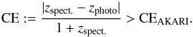
the percentage of catastrophic er-rors (CE), which meets the condition:
 (1)
(1) -
the estimated redshift accuracy, calculated as: | zspect−zphoto | /(1 + zspect.).
CE was defined by Ilbert et al. (2006) as the difference between photometric and spectroscopic redshifts largely greater than the expected uncertainty for the sample. The limiting redshift accuracy (CE = 0.15) was calculated by Ilbert et al. (2006) for the statistically significant sample of 3241 VVDS galaxies and based on the scatter between spectroscopic and photometric redshifts. For this sample the number of catastrophic errors increases with decreasing magnitude (in the case of the VVDS the redshift accuracy decreases by a factor of two between observed magnitude ranges 17.5 <i′< 21.5 and 23.5 <i′< 24). Regarding the ADF–S survey, as the number of spectroscopic measurements is very low, we are not able to calculate any statistically significant specific threshold for our sample. We decided to adapt an equation given by Rafelski et al. (2015), where the limiting value for the CE is calculated as:  (2)where
 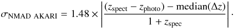 (3)CEAKARI calculated from Eqs. (2) and (3) is equal to 0.222, and: (1) is much bigger than the CE estimated by Ilbert et al. (2006) for the VVDS data, widely used in literature for different surveys (i.e., Speagle et al. 2016, Moutard et al. 2016, Castellano et al. 2016, Simm et al. 2015, Dahlen et al. 2013); and (2) we have only two galaxies with redshift accuracy >0.222 (which means almost no CEs in our sample). As our sample is not numerous, and the statistical significance of the obtained CEAKARI might be weak, we decided to use the threshold given by Ilbert et al. (2006) equal to 0.15 instead of the calculated value of 0.222, even though it is more conservative than ours. The number of CEs calculated with CEAKARI = 0.15 increases to eight (10%) in total.
Our mean redshift accuracy is equal to 0.056 (calculated as the normalized median absolute deviation2 =0.048), much lower than the one obtained by Ilbert et al. (2006) with Photometric Analysis for Redshift Estimate (Le PHARE, Arnouts et al. 1999; Ilbert et al. 2006), but this might be attributed to the much poorer statistics of our sample (95 galaxies) when compared to Ilbert et al. (2006, 2013) (3241 and 9389 galaxies, respectively). For a more detailed description of the ADF–S photometric redshift estimation process, we refer the reader to Małek et al. (2014).
Figure 1 shows the comparison of the full ADF–S spectroscopic sample (with nine additional sources not presented in Małek et al. 2014) with their photometric estimation. This figure presents a large group of galaxies with spectroscopic redshift and a failed estimation of the photometric value at z ~ 0.04. These galaxies are members of a nearby cluster, Abell S0463, one of several parts of the ADF–S field extensively observed in the past (Dressler 1980a,b; Abell et al. 1989). Incidentally, it is a redshift where almost all the existing tools for estimation of photometric redshifts experience a serious degeneracy (i.e., Fig. 10 of Bolzonella et al. 2000 for Hyperz tool; Fig. 3 of Ilbert et al. 2006; Fig. 1 of Ilbert et al. 2013 and Fig. 1 of Heinis et al. 2016 for lePhare tool). One of the reasons for the high fraction of CEs for galaxies at low redshifts could be the mismatch between the Balmer break and the intergalactic Lyman-alpha forest depression (for a more detailed discussion we refer the reader to Ilbert et al. 2006).
The scatter for a low zspec sample, visible in Fig. 1, can induce a large error in the luminosity distance (DL), and finally, cause possible inaccuracy of our analysis. To avoid this problem, we rejected all objects with spectroscopic or photometric redshift <0.05. With such a cut, the median difference between the luminosity distance, calculated for the spectroscopic and photometric redshifts for the presented sample as DL(zspec) /DL(zphot), is as low as 1.33 [Mpc] (the median absolute deviation =0.78). The redshift accuracy for the sample of galaxies with zspec ≥ 0.05 calculated as an arithmetic (as the distribution of the redshift accuracy is not Gaussian, and the number of objects is not high, we cannot calculate the mean and σ values) mean of | zspecti−zphotoi | /(1 + zspecti) (where i stands for each galaxy) equals 0.054 ± 0.024, and 78% of the sources have a redshift accuracy below this value (the redshift accuracy calculated as the normalized median absolute deviation is equal to 0.060), and in this case the number of CEs dropped down to two. We stress that, for the final sample, we used the same threshold both for spectroscopic and estimated photometric redshifts, and the obtained results are even better (redshift accuracy is equal to 0.050 with only one catastrophic error). To check how the redshift accuracy influences our final results, we ran the same analysis for all galaxies changing the value of the redshift ±0.05 (meaning that we do not show the worst effects of photometric redshift errors, but the mean influence of the uncertainty of the estimated zphot). This test is presented in Appendix A.
3. Sample selection and the properties of the final catalog
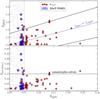 |
Fig. 1 Photometric versus spectroscopic redshifts and redshift accuracy versus spectroscopic redshift for a sample of 84 galaxies (red stars) for which the photometric redshift was calculated by Małek et al. (2014) using the CIGALE tool. Blue squares correspond to the Abell S0463 cluster. The region of CEs, defined as | zspec−zphoto | /(1 + zspec) > 0.15 (Ilbert et al. 2006), is marked by a solid black line. The navy dashed-dotted line corresponds to the zphot = zspec. Shadowed areas represent the redshift range rejected from our analysis. |
To construct the final ADF–S sample we restrict our analysis to sources with the best quality photometry available to fit SED models with the highest confidence. The main criterion was availability of redshift information (spectroscopic or photometric) in addition to at least six photometric measurements spanning the whole spectra. Additionally, we cut all objects with z< 0.05. In total, we selected 78 FIR-bright galaxies (22 galaxies with known spectroscopic redshift and 56 galaxies with redshifts estimated by CIGALE), with an average number of photometric measurements equal to 11.
Our sample is based on 90 μm detection and, therefore, each galaxy has at least one measurement in the FIR. What is very important for our method is that, in total, 27 ADF–S sources from the final sample have Herschel/SPIRE counterparts, allowing us to obtain very precise models of the FIR spectra, and to measure the real total dust temperature. All galaxies have measurements from WISE. 45 sources have Spitzer data (24 and 70 μm), and 56 have counterparts in the 2MASS catalog (Skrutskie et al. 2006). Unlike Małek et al. (2010), we did not use the IRAS data, as the uncertainties are too great and do not improve the SED fitting. We have also used the third release of the DENIS data (Paturel et al. 2003), and have found 55 counterparts for our selected sources. Almost 20% of our sample was detected in the UV GALEX bands. Thus, we are able to perform a multi-wavelength analysis of the ADF–S sources in order to build detailed SEDs from FUV to FIR, to get a range of physical properties of our sample.
Eight of our sources have 20 cm counterparts from the ACTA–AKARI survey. Unfortunately, two of them are unresolved (according to White et al. 2012, the ratio of the integrated flux density and peak flux density for unresolved sources is lower than 1.3). As for our SED fitting method, every additional model requires additional parameters. We decided to reject radio data from our analysis, since only six sources (3% of our sample) have reliable measurements in the 20 cm band.
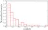 |
Fig. 2 Redshift distribution of the final sample of 78 ADF–S galaxies used for our analysis. |
The redshift distribution of our sample is shown in Fig. 2. From previous studies (Małek et al. 2010, 2014) we know that the ADF-S sample contains mostly nearby galaxies, whose properties are similar to the properties of the local population of optically bright, star-forming galaxies, except for having an unusually high ratio of peculiar (~10%) or interacting objects (Małek et al. 2010).
4. Methodology
Our main aim is to select and study LIRGs and ULIRGs to determine the main characteristics of their physical properties, and to use normal galaxies; the remaining sources from our catalog of 78 galaxies, not classified as LIRGs or ULIRGs, were used as a control sample. To achieve this goal it was very important to take into account the properties of the ADF–S galaxies along the whole wavelength range. We determined the main physical properties of FIR-bright galaxies form the AKARI survey by fitting their spectral energy distributions (SEDs), taking into account photometric information from UV to far infrared. We also decided to use additional, much simpler modeling based on the IR data only as a double check for ADF–S LIRGs and ULIRGs, and to derive the dust mass and dust temperature (not given from the Dale et al. 2014 model, used for the UV-FIR SED fitting). Also, we used CIGALE results as a reference.
4.1. UV to FIR SED-fitting
The SED fitting was performed using version v0.5 of the Code Investigating GALaxy Emission (CIGALE)3 developed with PYTHON, which provides physical information about galaxies by fitting SEDs that combine UV-optical stellar SED with a dust component emitting in the IR. CIGALE conserves the energy balance between the dust-absorbed stellar emission and its re-emission in the IR. The list of input parameters of CIGALE is shown in Table 1. We refer the reader to the CIGALE web page for a detailed description of the code.
4.1.1. Models
Star formation history
The SFHs used (optionally) by CIGALE are: (1) the double decreasing exponential star-formation history module (sfh2exp), which implements a SFH composed of two decreasing exponentials; (2) the delayed tau model, which implements a SFH described as a delayed rise of the SFR up to a maximum, followed by an exponential decrease; and the (3) custom module, which can be read from the file.
Input parameters of the code CIGALE.
Recently, Buat et al. (2014) published a comparison between SED fits obtained with two stellar populations. The comparison includes an exponentially decreasing/increasing SFR and a more complex SFR with two components: (1) the decreasing SFR for an old stellar population with and without a fixed value for the age of the oldest population; and (2) the younger burst of constant star formation. The conclusion was that when two stellar populations are introduced, fixing or not fixing the age of the oldest population, has only a modest impact, and two populations still give the best fit to the data.
Thus, we assume a similar SFH to Buat et al. (2014). In our analysis we adopted an exponentially decreasing SFR for the old and young stellar populations. A similar approach was used by Erb et al. (2006), Lee et al. (2009), Buat et al. (2011), Giovannoli et al. (2011), and Ciesla et al. (2015).
Single stellar population
CIGALE uses the stellar population synthesis models either by Maraston (2005) or Bruzual & Charlot (2003). For this work we adopted the stellar population synthesis models of Maraston (2005), as they consider the thermally pulsating asymptotic giant branch (TP-AGB) stars. This model includes young stellar population tracks from the Geneva database, and the Frascati database for older populations (for a more detailed discussion we refer the reader to Maraston 2005; and Maraston et al. 2009). In general, Maraston (2005) models provide reliable information on the NIR-bright stellar population of galaxies, which is very important for our analysis, since our sources have been detected in the NIR bands. To calculate the initial mass function (IMFs), CIGALE has two built-in algorithms based on Salpeter (1955) and Kroupa (2001) models.
Attenuation curve
The galaxy attenuation curve adopted by CIGALE is based on the Calzetti law (Calzetti et al. 2000) with some modifications (for a more detailed discussion we refer the reader to Noll et al. 2009). CIGALE allows the user to alter the steepness of the attenuation curve and/or to add a UV bump centered at 2175 Å (Noll et al. 2009). We did not modify the Calzetti law, but we use three different values for E(B−V), which represent the attenuation of the youngest population, and the reduction factors are applied to the color excess of stellar populations older than 107 yr.
Dust emission
The new version of CIGALE includes four different models to calculate dust properties: Casey (2012), Dale et al. (2007, 2014), and an updated Draine & Li (2007) model. Since we decided to use the Casey (2012) model for a double-check of CIGALE, the main dust analysis was based on the Dale et al. (2014) model, which is the most suitable for very luminous infrared sources. The results given by Dale et al. (2014) are
-
the fraction/contribution of an AGN to the mid infrared spectrum,
-
the slope of the infrared part of the spectrum – parameter α – empirically determined by Dale & Helou (2002) based on the ratio of IRAS fluxes detected at 60 and 100 μm (the model was improved by Dale et al. 2014). It describes the progression of the FIR peak toward shorter wavelengths for increasing global heating intensities. Parameter α ranges from 0.0625 to 4, as the dust heating changes from strong to quiescent (Dale et al. 2005). The lower the value of α, the more actively star forming a galaxy is. Normal galaxies display 1 <α< 2.6, while α~ 2.5 characterizes an already quiescent galaxy (Dale et al. 2001; Dale & Helou 2002). Values of α~ 4 are typically fitted for galaxies where the FIR emission peak appears at even longer wavelengths than for the most quiescent, well studied, galaxies and corresponds to the coolest and most quiescent galaxies,
-
the total IR luminosity between 8 and 1000 microns (Ldust), defined as the sum of stellar and AGN luminosities re-processed by dust.
Dale et al. (2014) presented an updated version of the model originally proposed by Dale & Helou (2002). This model describes the progression of the FIR peak toward shorter wavelengths for increasing global heating intensities (Dale et al. 2001). CIGALE adopts 64 templates of Dale et al. (2014) models. All models are parametrized by the α parameter.
The main improvements between versions presented by Dale & Helou (2002) and Dale et al. (2014) are: (1) the MIR parts of the models, originally based on the ISOPHOT data from the Infrared Space Observatory were rebuilt using the data from the Spitzer Space Telescope; and (2) the AGN component has been included to compose the total infrared luminosity. For the updated MIR spectrum the 5−34 μm “pure” star-forming curve from Spoon et al. (2007) was adopted; it makes use of the Spitzer data to model a sequence of MIR spectral shapes for AGNs, LIRGs and ULIRGs, and star-forming galaxies.
The Dale et al. (2014) model can also derive a fraction of AGN that contributes to the galaxy dust luminosity in MIR. Unfortunately, this model is more suitable for broad-line AGNs, and additionally, does not include any absorption features (e.g., 9.7 μm, characteristic for ULIRGs), and thus, the AGN components estimated by this model can be misleading. A lack of the 9.7 μm absorption line does not affect an α parameter as the AKARI ADF–S sample has very good coverage between MIR and FIR wavelengths, sufficient to calculate a proper slope. Since our aim is to look for the presence of both Type 1, Type 2, and intermediate types of AGNs in our sources, we decided to use Dale et al. (2014) templates to estimate global heating intensities and dust luminosity values only. We have adopted the Fritz et al. (2006) model to check the fractional contribution of AGNs to the MIR emission.
AGN emission
The latest release of CIGALE includes Fritz et al. (2006) models of AGN emission. Fritz et al. (2006) created an improved model for the emission from dusty torus heated by a central AGN. In this model a flared torus is defined by its inner and outer radii and the total opening angle (θ). The adopted density of dust grain distribution depends on the torus radial coordinate and polar angle, and the optical depth is computed taking into account the different sublimation temperatures for silicate and graphite grains. The templates are computed at different lines of sight with respect to the torus equatorial plane (ψ) in order to account for both Type 1 and Type 2 emission, from 0° to 90°, respectively, in steps of 10°. Very important for our analysis is that Fritz et al. (2006) models preserve the energy balance which perfectly matches the method used by CIGALE.
This model gives a good estimation for Type 1 and Type 2, as well as for the intermediate types of MIR SED of AGNs, even for non-numerous photometric data (Feltre et al. 2012, and references therein). According to the convention used by Fritz et al. (2006), the angle ψ between the AGN and the line of sight for the extreme cases of Type 1 and Type 2 AGNs is equal to 90° and 0°, respectively. For a detailed description of the Fritz et al. (2006) model we refer the reader to the original paper.
The first usage of Fritz et al. (2006) templates in CIGALE was reported by Buat et al. (2015), and Ciesla et al. (2015). Buat et al. (2015) used Fritz et al. (2006) templates as an additional model to built SEDs of real galaxies from the AKARI North Ecliptic Pole Deep Field, while Ciesla et al. (2015) analyzed simulated realistic SEDs of Type 1, Type 2, and intermediate types of AGNs to estimate the ability of CIGALE to retrieve the physical properties of the galaxy, and to calculate possible under- and over-estimations of AGN fraction, stellar masses, and star formation parameters obtained from the SED fitting.
Ciesla et al. (2015) showed the difference between flux density ratio of SEDs with and without AGN emission for Type 1, Type 2 and intermediate types of AGNs (Ciesla et al. 2015, Fig. 4), which can be reckoned as the main description of different types of AGN influence on the full spectra fitting. As it was shown by Ciesla et al. (2015), based on the model introduced by Fritz et al. (2006) for the UV-FIR SED fitting method, Type 1 AGNs are chosen based on the higher emission in the UV and MIR rest-frame spectra, compared to the same SED without the AGN component. The main characteristic assumption for selection of Type 2 AGNs is the amplified MIR and FIR emission. The ADF-S sample was selected based on the FIR bands, and all galaxies used for the analysis have measurements spanning the whole spectral range. As a result, parts of the spectrum needed for AGN identification are sufficiently well covered, thus, Type 1, Type 2, and intermediate types of AGNs can be easily recognized based on the SED fitting.
For our analysis, we have used four Fritz et al. (2006) templates built based on average parameters from previous studies of the model (i.e., Hatziminaoglou et al. 2008, 2009, Buat et al. 2015, Ciesla et al. 2015). These parameters are: (1) the ratio of the outer to inner radius of the torus fixed to 60.0; (2) the radial and angular dust distribution in the torus equal to −0.5, and 0.0, respectively; and (3) the angular opening angle of the torus fixed to 100 [deg]. To follow the low and the high optical depth at 9.7 μm, two values of (τ9.7) were chosen: 1.0 and 6.0. These values of τ9.7 are consistent with results presented by Ciesla et al. (2015) and Buat et al. (2015), as well as our internal tests. To consider the most extreme cases of AGNs (Type 1 and Type 2) we used the values of an angle between equatorial axis and the line of sight equal to 0.001 and 89.990 degrees. Four selected templates used in the further analysis are plotted in Fig. 3.
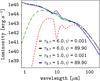 |
Fig. 3 Fritz et al. (2006) AGNs’ SEDs used in our analysis. These templates are built based on two optical depth τ9.7 values (1.0 and 6.0), and the extreme values of the angle between the equatorial axis and the line of sight (ψ). The red dotted line represents τ9.7 = 1.0, and ψ = 89.900 [deg]; the green dashed line corresponds to the τ9.7 = 1.0, and ψ = 0.001 [deg]; the black dashed-dotted line to τ9.7 = 6.0, and ψ = 89.900 [deg]; and the blue solid line to τ9.7 = 6.0, and ψ = 0.001 [deg]. |
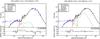 |
Fig. 4 Examples of the best fit models (CIGALE SED fitting code). The left-hand side spectrum is a star-forming galaxy, while the spectrum shown on the right-hand side is ULIRG. Observed fluxes are plotted with open blue squares. Filled red circles correspond to the model fluxes. The final model is plotted as a solid black line. The remaining three lines correspond to the stellar, dust, and AGN components. The relative residual fluxes are plotted at the bottom panel of each spectrum. |
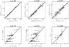 |
Fig. 5 Pearson product-moment correlation coefficient (r) calculated between ADF–S galaxies and the corresponding mock catalog (created from the input values) for dust luminosity, SFR, stellar mass, dust attenuation in V and FUV bands, and α parameter of the model of Dale et al. (2014). The calculated values of r are written above each plot. |
4.1.2. Modeled SEDs
The quality of the fitted SEDs is calculated making use of the χ2 value of the best model, marginalized over all parameters except the one assigned for the further physical analysis. In the next step, the values of the probability distribution function (PDF) of the derived parameters of interest (in the case of this paper: Mstar, Ldust, AGN fraction, the AGN torus angle with respect to the line of sight, α slope of the model Dale et al. (2014), and SFR are calculated. The final output values of analyzed parameters are calculated as the mean and standard deviation determined from the PDFs (Ciesla et al. 2015; Buat et al. 2014; Burgarella et al., in prep.; Boquien et al., in prep.; see also Walcher et al. 2008, for more detailed explanation of the χ2 – PDF method).
Based on the distribution of χ2 values for the ADF–S sample we decided to restrict our analysis to the modeled SEDs with the reduced χ2 value lower than five. The threshold value was chosen as a mean χ2 + 3σ. We found 71 galaxies that fulfill this condition for the χ2.
After visual verification of all single fits, we decided to remove two objects with a satisfying χ2 from the further analysis because of a poor photometric coverage of the spectra. Namely, (1) object IDADFS = 148 has the minimal number of photometric measurements required for the analysis (six) but only one located in the infrared part of the spectrum (from the 90 μm AKARI band). This object has no Herschel counterpart and only one photometric point from the WISE; (2) object IDADFS = 281 has a similar distribution of photometric data but with a total number of nine measurements. In both cases, the stellar part is very well fitted, but the infrared part is rather an estimate of the real shape of the spectrum.
Finally, we restricted the final sample to 69 galaxies (among them, 20 objects with known spectroscopic redshift and 49 galaxies with photometric redshift) that fulfill the χ2 and visual inspection conditions.
Examples of the best fit models for the ADF–S galaxy sample are shown in Fig. 4.
4.1.3. Reliability check
The mock catalog was generated to check the reliability of the computed parameters. To perform this test we used an option included in CIGALE, which allows for creation of mock objects for each galaxy. The final step of verification of estimated parameters is to run CIGALE on the mock sample using the same set of input parameters as for the real catalog, and to compare the output physical parameters of the artificial catalog with the real ones. A similar reliability check was performed for example by Giovannoli et al. (2011), Yuan et al. (2011), Boquien et al. (2012), Małek et al. (2014), and Ciesla et al. (2015).
Figure 5 presents the comparison of the output parameters of the mock catalog created from the input parameters versus values estimated by the code for our real galaxy sample. The determinant value, which can characterize the reliability of the obtained values, is the Pearson product-moment correlation coefficient (r). The comparison between the results from the mock and real catalogs shows that CIGALE gives a very good estimation of main physical parameters which we use for the final analysis (Ldust, SFR, Mstar, fraction of AGN, and α parameter from the Dale et al. 2014 model). For dust attenuation in V and FUV bands, the correlation is not obvious. Consequently, we only used the results to present a general trend of how the dust component affects the stellar part of the spectra.
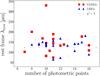 |
Fig. 6 Number of photometric points used for CIGALE fitting vs. the peak of the dust part of the spectra (λmax for 156 ADF–S objects fitted with χ2< 10). Filled red squares represent ULIRGs, filled blue traingles represent LIRGs, and the gray “x”-s correspond to normal star-forming galaxies. As the λmax corresponds to the dust temperature, we conclude that we do not find any degeneracy with respect to the number of photometric points in the estimation of the peak of the dust part of the spectrum. |
We have also examined how the peak of the dust part of the spectra (λmax, related to the dust temperature) depends on the number of photometric points used for the SED fitting. Figure 6 shows the relation between the number of photometric measurements and λmax relation for our sample of 69 galaxies with a marked dependence on the total dust luminosity. We did not find any degeneracy in this relation. Based on this figure we conclude that the significant percentage of LIRGs and ULIRGs selected based on the 90 μm AKARI band compose cold sources, as only five of them (~12%) have λmax<90 μm. Our results are in agreement with Symeonidis et al. (2011).
We have also examined how the number of photometric points affects other physical properties estimated by CIGALE, and we did not find any significant correlation. We performed a similar test to examine whether or not the photometric redshifts estimated by Małek et al. (2014) depend on the number of photometric measurements, but we found (similarly to the λmax parameter) a flat relation without any significant dependence on the number of photometric points that fulfill our initial conditions. We conclude that our final selection (galaxies with photometric points covering the whole spectrum from FUV to FIR, with more than two measurements between 8 and 1000 μm, and at least three measurements in the UV-to-optical part of the spectrum for the final sample of 69 ADF–S objects) gives us very good coverage of the spectral energy distribution, sufficient for a reliable fit.
In the ADF–S sample, we found 17 galaxies (24% of the sample) that can be classified as ULIRGs. They are mostly galaxies with photometric redshifts; only one galaxy (HE 0435-5304) has a known spectroscopic redshift; it is the most distant galaxy from our sample, detected at z = 1.23 (Wisotzki et al. 2000) and classified as quasar by Véron-Cetty & Véron (2006). The interesting point about HE 0435-5304 is that Keeney et al. (2013) found a different spectroscopic redshift using the data from the Cosmic Origins Spectrograph installed aboard the Hubble Space Telescope (HST); based on the Lyα and NV emission lines, the spectroscopic redshift for HE 0435-5304 was found to be equal to 0.425. Now, with additional data we were able to estimate zphot, and we obtain zphot = 0.30, and the redshift accuracy calculated for HE 0435-5304 between Keeney et al. (2013) and our photometric value equals 0.125. For zspec = 1.23 we obtain an extremely bright ULIRG (or the lower limit HLIRG, taking into account the uncertainties, with log (Ldust) = 13.12 ± 0.29 [L⊙]). The physical properties of this object, based on the “official” high redshift, always make it an outlier with respect to the whole ULIRG sample as seen from Figs. 11, 15, and 21, for example. Properties of the same object, calculated with a new redshift z = 0.43, give us a typical LIRG (log (Ldust) = 11.12 ± 0.09 [L⊙]) with physical parameters characteristic for the LIRG sample. As the previous redshift (1.23) is given by the NED and other public databases, we decided to present the results based on the reference, but we point out that the results obtained with the lower redshift by Keeney et al. (2013) appear much more reasonable.
In the sample, 22 galaxies (32%) were classified as LIRGs (including five galaxies with known spectroscopic redshift). This means that LIRGs and ULIRGs in total compose 56% of the bright ADF–S sample at redshift >0.05.
The control sample contains 30 normal galaxies (12 of them have spectroscopic redshift).
We note that in our sample of LIRGs and ULIRGs, only one LIRG (IDADFS = 46) and one ULIRG (IDADFS = 212) have only eight photometric measurements. The average number of photometric points for the final sample of 39 objects is equal to 12. It means that the spectra are well defined by the measurements, and the models are well fitted.
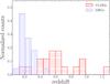 |
Fig. 7 Normalized redshift distribution of 22 ADF–S LIRGs (vertical striped blue histogram) and 17 ULIRGs (horizontal striped red histogram). |
Redshift distribution of ADF–S galaxies with Ldust> 1011 [L⊙] is shown in Fig. 7. The mean values of redshift for ADF–S LIRGs and ULIRGs are equal to 0.23 ± 0.08 and 0.61 ± 0.26, respectively. This implies that ADF–S LIRGs are mainly objects from the local Universe, while ULIRGs are more commonly found at higher redshift. A similar distribution of LIRGs and ULIRGs was found by Lin et al. (2016) for galaxies selected at 70 μm Spitzer MIPS band: the majority of ULIRGs were found on a higher redshift than LIRGs and star-forming galaxies.
Main physical parameters for ULIRGs, LIRGs, and galaxies with total infrared luminosity LTIR< 1011L⊙ from the ADF–S sample derived by CIGALE and CMCIRSED.
We have also checked the angular deviation between the found LIRGs and ULIRGs and their optical counterparts. Three LIRGs have angular distances between optical counterparts and AKARI measurements at 90 μm larger than 20′′: 20.36′′, 24.36′′, and 30.06′′ for IDADF−−S equal to 6, 93, and 203, respectively. One ULIRG (IDADF−−S = 59) has an angular distance equal to 21.24′′. However, the mean angular distance for both LIRGs and ULIRGs is equal to 8.94′′ with a standard deviation of 6.20 arcsec (median value 8.20′′). We claim that only one source, a LIRG with IDADF−−S = 203, might be unreliable, but its SED is, overall, well fitted, and the obtained physical parameters are reasonable (see Table A.2).
The final catalog of 39 LIRGs and ULIRGs used for our analysis is given in Table A.1 available at the CDS. The catalog contains the following information: Col. 1 lists the ADF–S name of the source, Cols. 2 and 3 give the coordinates, Col. 4 provides the redshift, Col. 5 lists the redshift references, Col. 6 gives 46 photometric flux densities and uncertainties for 20 bands spanning spectra from FUV (GALEX) to FIR (Herschel/SPIRE), and Col. 47 gives the name of the nearest optical counterpart. An example of two rows from the final catalog are shown in Table A.1, at the end of this paper.
This significant percentage of galaxies, with  in the ADF–S sample, can be related to the fact that most of our galaxies (more than 55%) were also detected at 24 μm, and the 24 μm band is a well-known tracer of active, star-forming galaxies (e.g., Calzetti et al. 2007).
Table 2 shows the mean values of physical parameters calculated for LIRGs and ULIRGs obtained from the UV to FIR SED fitting, while Fig. 10 shows their distributions. The discussion, and comparison of the parameters listed in Tables 2 and A.2 are presented in the following subsections with corresponding citations.
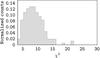 |
Fig. 8 χ2 distribution for the ADF-S sample obtained from CMCIRSED code. One galaxy with χ2> 70 is not shown on this histogram. |
4.2. CMCIRSED: NIR to FIR SED-fitting
The Caitlin M. Casey Infra Red Spectral Energy Distribution model (CMCIRSED4) published by Casey (2012), uses the single temperature gray-body + MIR power law, which was demonstrated to work very well for the FIR galaxy spectrum (for the wavelength range 8 μm <λ< 1000 μm). We perform the SED fitting with the CMCIRSED model as a double-check for ADF–S LIRGs and ULIRGs, as well as to compute the dust mass and dust temperature for our sample, which is not given by the CIGALE models we used for our analysis.
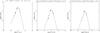 |
Fig. 9 Three examples of the best-fit models by CMCIRSED shown from left to right: ULIRG, LIRG, and a normal galaxy. |
The SED-fitting procedure of the CMCIRSED model requires two free parameters: the slope coefficient (α), and emissivity (β). We performed many tests for α and β to obtain the optimal SEDs for the ADF–S sample. For α (a power law slope coefficient) we adopted a range from 1.5 to 2.5, and for the spectral emissivity index (β) we used values from 1.2 to 1.8. For a more detailed description of these parameters we refer the reader to Casey (2012).
CMCIRSED gives the residuals of the fits as the difference in the flux density at the rest-frame frequency between the data points and the best-fitting SED at 12, 25, 60, 100, and 850 μm wavelengths (Casey 2012). To make both parts of the analysis (CIGALE and CMCIRSED SED fitting) homogeneous, we added an additional procedure to the cmcirsed.pro code that computes the reduced χ2 value for the best-fit FIR spectrum. Figure 8 shows the distribution of the reduced χ2 values for the ADF–S sample.
Based on the presented histogram (Fig. 8) and the visual inspection of the obtained infrared SEDs, we decided to restrict our analysis to the galaxies for which the reduced χ2 value was lower than 13.1 (according to the distribution, χ2 equal to 13 should be a threshold for this code, but the visual inspection of each individual SED increased the number of selected sources by one; an additional LIRG with a marginal value of χ2 = 13.08. We used 124 galaxies as the final sample for the subsequent analysis which fulfilled this condition. Three examples of SED fits for the ADF–S galaxies are shown in Fig. 9.
Based on the CMCIRSED model and an additional threshold for the reduced χ2 value, we found 12 ULIRGs and 13 LIRGs (25 galaxies in total, which corresponds to 22% of the ADF–S galaxies with reliable CMCIRSED SED fits). For nine LIRGs and five ULIRGs found by CIGALE (14 objects in total) it was not possible to perform a satisfactory fitting using a CMCIRSED code. For four of them, the number of IR measurements was simply too low to perform a reliable fit (three to four photometric points). For three galaxies, the reduced χ2 was too high to use them for the further analysis, and for the remaining objects, the fitted dust temperature was either lower than 10 K (and at the same time, the uncertainties were equal to 0) or the estimated errors were much higher than 50% of the dust temperature value. We excluded them from the final analysis. We stress that none of the LIRGs and ULIRGs identified by CIGALE were identified as normal galaxies by CMCIRSED, but rather CMCIRSED was unable to perform a reliable fit to their SEDs. This discrepancy between the results given by both codes is well explained as the lack of Herschel/SPIRE data for some galaxies, since FIR data are crucial for a code based on the FIR data only. CIGALE has the advantage over CMCIRSED in the cases where the IR measurements between 8 and 1000 μm are scarce. In such cases CIGALE can estimate properties of galaxies based on the composed models from the stellar and NIR–MIR part of the spectrum, while the fitter, based on the IR data, has only limited capabilities to deduce a real character of the analyzed object.
Infrared luminosity, dust temperature, and dust mass of galaxies, along with α and β parameters, were derived from the CMCIRSED model. The reliable LIRGs and ULIRGs, identified by this code, together with their physical parameters, are listed in Table A.2. Mean values for ULIRGs, LIRGs, and normal galaxies derived from the Casey (2012) model are presented in Table 2.
5. LIRGs and ULIRGs main physical properties obtained from the SED fitting processes
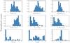 |
Fig. 10 Distribution of physical properties obtained by CIGALE for the ADF–S galaxies: dust luminosity (Ldust), star formation rate (SFR), specific SFR, stellar mass (Mstar), dust attenuation in V and FUV bands, fractional contribution of AGN to the MIR emission (AGNfract), AGN’s torus angle with respect to the line of sight (ψ), IR spectral power-law slope α. |
5.1. Dust luminosity
As mentioned above, the dust luminosity of the ADF–S galaxies was calculated based on the Dale et al. (2014) model. The median dust luminosity is equal to 1010.30 ± 101.07 [L⊙]. From the Ldust distribution (Fig. 10 top left panel) one can clearly recognize three peaks: (1) a very broad sample of normal star-forming galaxies, with a maximum located at approximately 1010 [L⊙]; (2) a much narrower distribution of galaxies with log (Ldust)~ 11.3 L⊙; and (3) a group of ultra bright galaxies, with the peak of log (Ldust) distribution near 12.40 [L⊙], and the tail shifted towards very bright sources (HLIRGs: hyper LIRGs).
To examine how the extremely dusty component affects the stellar part of the spectra we have calculated their dust attenuation. With CIGALE we are able to calculate the amount of obscuration of stellar luminosity for the old stellar population using V and FUV filter measurements. As the correlation between ADF–S results and the mock catalog has a large scatter, we decided to check only the general trend for this relation. We have found that the dust attenuation for the old stellar population is not strong and has a similar value for normal galaxies, LIRGs, and ULIRGs, that is, ~0.7 [mag]. The same conclusion might be drawn from exemplary SEDs shown in Fig. 4, where it is difficult to distinguish between unattenuated and attenuated stellar components for the old stellar population.
Our results show that the shape of the spectrum from the old stellar population almost remains the same, and only in the ultraviolet wavelengths, related to the emission from young stars, stellar spectra are obscured on the average level of 3 mag (Fig. 13, and Fig. 4 – example SEDs). Our findings are inconsistent with da Cunha et al. (2010) for 16 ULIRGs preselected from the IRAS 1 Jy survey, observed in the 5–38 μm range by Spitzer/IRS. To estimate the dust attenuation da Cunha et al. (2010) used the strength of the 9.7 μm silicate feature from the Spitzer/IRS MIR spectra, and converted them to the V-band optical depth by assuming dust optical properties and geometry. da Cunha et al. (2010) found that, for ULIRGs, the V-band optical depth is very large (mean  = 33.49 ± 7.14), and the shape of the stellar spectrum is distorted by dust attenuation (da Cunha et al. 2010,Fig. 3).
This alternative impact on the shape of the old stellar populations is due to the difference in the attenuation curve adopted in the MAGPHYS code used by da Cunha et al. (2010) and in the version of CIGALE used here. The MAGPHYS method leads to a flatter attenuation curve than the Calzetti law adopted here (Chevallard et al. 2013) and implies a higher mean attenuation, which also affects the NIR spectrum and the contribution of the old stellar population (Lo Faro et al., in prep.).
5.2. Stellar mass
ADF–S galaxies are relatively massive with the median value of Mstar equal to 109.38 ± 100.38 [M⊙]. The mean Mstar computed for ULIRGs, LIRGs, and galaxies with log (Ldust) < 11 [L⊙] is equal to 11.51 ± 0.37, 10.35 ± 0.31, and 10.03 ± 0.50 [M⊙], respectively. Stellar masses computed by CIGALE for the ADF–S sample are consistent with stellar masses calculated for LIRGs and ULIRGs located at similar redshifts, selected from infrared surveys and published by:
-
U et al. (2012); found 53 LIRGs and11 ULIRGs from the Great Observatories All-sky LIRG Survey(GOALS, Armuset al. 2009) at redshift0.012 <z< 0.083. They found mean stellar mass for LIRGs equal to log (MLIRGsstar) = 10.75 ± 0.39 [M⊙], and for the ULIRGs: log (MULIRGsstar) = 11.00 ± 0.40 [M⊙].
-
Pereira-Santaella et al. (2015); described 29 local systems and individual galaxies with infrared luminosities between 1011 and 1011.8[L⊙], selected from IRAS Revised Bright Galaxy sample (Sanders et al. 2003). Among the UV to FIR SED fitting results presented by Sanders et al. (2003) (Table 7), we found 19 LIRGs with a mean stellar mass equal to 10.82 ± 0.32 [M⊙], and median value =10.88 [M⊙].
-
Stellar masses estimated for ULIRGs are also consistent with Rothberg et al. (2013) dynamical masses calculated for eight local (z< 0.15) ULIRGs, randomly selected from a sample of 40 objects taken from IRAS 1 Jy Survey. The mean dynamical mass at I-band for ULIRGs obtained by Rothberg et al. (2013) is equal to 11.64 ± 0.32.
We have also compared our results with more distant galaxies, reported by:
-
Giovannoli et al. (2011); 62 LIRGsfrom the Extended Chandra Deep Field South, selected at24 μm, on redshift ~0.7 with the log (Mstar) between 10 and 12 [M⊙], and with a peak at 10.8 [M⊙].
-
Melbourne et al. (2008); who calculated the stellar masses for 15 LIRGs from the GOODS-S HST treasury field; For this sample of LIRGs, with redshift ~0.8, the mean stellar mass equals log(Mstar)~ 10.51 [M⊙].
-
Santos et al. (2015); for 12 XDCP J0044.0-2033 cluster members at redshift 1.58 observed by Herschel. For the sample of 12 ULIRGs, we have found the mean log (Mstar) = 11.06±0.32 [M⊙].
-
We also compared our results with the stellar masses for 122 sub-millimeter galaxies (SMGs), with median photometric redshift equal to 2.83 reported by da Cunha et al. (2015). We selected ULIRGs and LIRGs from the SMG sample, and found their mean log(Mstar) for 88 ULIRGs equal to 10.88 ± 0.51 [M⊙], while for 8 LIRGs: mean log(Mstar) was equal to 9.77 ± 0.52 [M⊙].
In both cases (local, and more distant Universe), the stellar masses for the LIRGs and ULIRGs we found in the ADF–S data are consistent with the literature. Both our results and results reported in the literature suggest that LIRGs and ULIRGs are more massive than normal galaxies, and that their stellar masses increase with infrared luminosity.
5.3. IR power-law slope
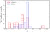 |
Fig. 11 Histogram of the α parameter from Dale et al. (2014) model. The horizontal striped red histogram represents ULIRGs while the vertical striped blue histogram corresponds to LIRGs. |
Figure 11 shows the distribution of α parameter (Dale & Helou 2002) for the ADF–S LIRGs and ULIRGs. It demonstrates that our sample consists mostly of galaxies active in star formation. Only five ULIRGs have α> 2. One of them is the most distant galaxy from our sample, a quasar, with known spectroscopic z = 1.23, with α = 3.15 ± 0.47. Unfortunately, for this galaxy we have no Herschel/SPIRE data which implies that the temperature of dust may be not well evaluated.
Nevertheless, more than 80% of ULIRGs, and 95% of LIRGs are characterized by a low value of α. Taking into account a high reliability of the α parameter (the Pearson product-moment correlation coefficient with mock catalog is equal to 0.95, Fig. 5), it is possible to draw the conclusion that LIRGs and ULIRGs are very active in star formation. Furthermore, based on the distribution of α parameter between different groups of sources, we can conclude that LIRGs and ULIRGs are characterized by a stronger starburst activity than normal galaxies.
The mean value of α is lower for ULIRGs than for LIRGs, but taking into account the uncertainties we cannot distinguish both groups based on this parameter. Values of α computed for ULIRGs, LIRGs and normal galaxies are listed in Table 2.
5.4. Star-formation rate
We checked the distribution and the median values of the SFR for our sample. Values of SFR for ADF–S LIRGs and ULIRGs vary from 13.45 to almost 2900 [M⊙ yr-1] (the latest for the extreme case of a quasar at zspec = 1.23), with the median value equal to 65.58 [M⊙ yr-1].
For ULIRGs, LIRGs, and the rest of the galaxies from our sample, the mean log (SFR)ULIRG, log (SFR)LIRG, and log (SFR)normal are equal to 2.53 ± 0.39, 1.47 ± 0.20, and 0.47 ± 0.21 [M⊙ yr-1], respectively (Table 2). Our results are consistent with the Kennicutt (1998) relation between SFR and dust luminosity: ![Mathematical equation: \begin{equation} {\it SFR}~[M_{{\odot}~{\rm yr}^{-1}}]=4.5\times10^{-44} \times L_{\rm dust} [{\rm erg~s^{-1}]}, \label{eq:Kennicutt98} \end{equation}](/articles/aa/full_html/2017/02/aa27969-15/aa27969-15-eq133.png) (4)where Ldust refers to the infrared luminosity integrated over the full MIR and fIR spectrum (8–1000 μm). Figure 12 shows the SFR−Ldust distribution of ADF–S galaxies with an additional black line which represents Eq. (4). We conclude that our results are in very good agreement with the Kennicutt (1998) relation, and the SFR increases with dust luminosity in the same way for normal galaxies, LIRGs, and ULIRGs.
(4)where Ldust refers to the infrared luminosity integrated over the full MIR and fIR spectrum (8–1000 μm). Figure 12 shows the SFR−Ldust distribution of ADF–S galaxies with an additional black line which represents Eq. (4). We conclude that our results are in very good agreement with the Kennicutt (1998) relation, and the SFR increases with dust luminosity in the same way for normal galaxies, LIRGs, and ULIRGs.
Our results for the LIRGs and ULIRGs are consistent with those presented in the literature, that is;
-
Santos et al. (2015):⟨ log (SFR)ULIRGs ⟩ = 2.51 ± 0.22 [M⊙ yr-1];
-
Podigachoski et al. (2015): ⟨ log (SFR)ULIRGs ⟩ = 2.55 ± 0.26 [M⊙ yr-1];
-
da Cunha et al. (2015): ⟨ log (SFR)ULIRGs ⟩ = 2.55 ± 0.32, and ⟨ log (SFR)LIRGs ⟩ = 1.69 ± 0.20 [M⊙ yr-1]; and
-
Howell et al. (2010) (181 LIRGs and 21 ULIRGs on the median redshift 0.008 and a maximum redshift equal to 0.088): ⟨ log (SFR)ULIRGs ⟩ = 2.45 ± 0.14 [M⊙ yr-1], and ⟨ log (SFR)LIRGs ⟩ = 1.72 ± 0.69 [M⊙ yr-1].
Figure 13 shows the correlation between SFR and stellar mass for the ADF–S sample. We have over-plotted the SFR–Mstar relation found by Noeske et al. (2007) for All-Wavelength Extended Groth Strip International Survey galaxies (AEGIS) at redshift range from 0.2 to 0.7, and Elbaz et al. (2007) for Great Observatories Origins Deep Survey (GOODS), at z ~ 1. We can compare these results to ours since both the sample selection and redshift range (0.2−0.7) are similar. We found that the majority of ADF–S ULIRGs are located above the observed linear correlation from Noeske et al. (2007) and Elbaz et al. (2007). LIRGs are also shifted towards higher SFR, and the trend is consistent with Noeske et al. (2007). The minimal value of log(SFR) for our LIRGs is equal to 1.0 ± 0.2 [M⊙ yr-1], and is consistent with their LIRG SFR limit obtained by Noeske et al. (2007).
5.5. Specific star-formation rate
We also calculated specific star-formation rate (SSFR), which is defined as the ratio between SFR and the total stellar mass of a galaxy:![Mathematical equation: \begin{equation} {\it SSFR} = {\it SFR}/M_{\rm star}~[{\rm yr}^{-1}]. \end{equation}](/articles/aa/full_html/2017/02/aa27969-15/aa27969-15-eq138.png) (5)The median values of SSFR for ADF–S ULIRGs, LIRGs, and normal galaxies are equal to −8.98 ± 0.47, −9.48 ± 0.45, and −9.56 ± 0.38 [yr-1], respectively (Table 2). These values indicate that the SSFR increases with dust luminosity.
(5)The median values of SSFR for ADF–S ULIRGs, LIRGs, and normal galaxies are equal to −8.98 ± 0.47, −9.48 ± 0.45, and −9.56 ± 0.38 [yr-1], respectively (Table 2). These values indicate that the SSFR increases with dust luminosity.
We compared our results to the ones presented in the literature for LIRGs and ULIRGs selected in the infrared. The median value of SSFR for ULIRGs in the GOALS field (Howell et al. 2010) is equal to −9.41 [yr-1], while U et al. (2012) obtained a value of −9.17 [yr-1]. Our results are consistent with both of them.
On the other hand, da Cunha et al. (2015) found SSFRULIRGs=−8.32±0.49[yr-1] which is also consistent with ours, but their SSFR for LIRGs is higher than the one obtained for the ADF–S (SSFRLIRGs = −8.08±0.38[yr-1]). This discrepancy might be caused by a small number of objects (da Cunha et al. 2015 sample consists of only eight LIRGs) and their much-higher redshift (mean photometric redshift equal to 1.90). Another possibility is the use of a flatter attenuation curve than the Calzetti law (last paragraph of Sect. 5.1, and Lo Faro et al., in prep.).
The mean SSFR calculated for 19 local LIRGs presented by Pereira-Santaella et al. (2015) is equal to −10.60 ± 0.45 [yr-1], and this value is lower than the other values from the literature. It might be caused by the different sample selection or statistical differences between samples. The results obtained for the ADF–S sample are statistically consistent with the results from Howell et al. (2010), U et al. (2012), and Pereira-Santaella et al. (2011).
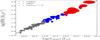 |
Fig. 12 Dust luminosity versus SFR for ADF–S sample. Filled red squares represent ULIRGs, filled blue triangles correspond to LIRGs, and the filled gray circles represent normal galaxies with log (Ldust) < 11 [L⊙]. The radius of an ellipse represents error bars for dust luminosity, and SFR, respectively. The black line corresponds to the Kennicutt (1998) SFR, i.e., the dust luminosity relation. |
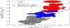 |
Fig. 13 Stellar mass versus SFR for ULIRGs (filled red ellipses), for LIRGs (filled blue ellipses), and for normal galaxies (filled gray ellipses). The black solid line represents log (Mstar): log (SFR) relation given by Noeske et al. (2007) for galaxies at redshift ≃ 0.6, when dashed line corresponds to Elbaz et al. (2007) relation for galaxies at z ≃ 1. |
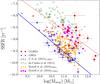 |
Fig. 14 Relationship between SSFR and stellar mass for ULIRGs and LIRGs derived from this work. Lines represent the linear fit for ULIRGs (red dotted line) and LIRGs (blue solid line) from the ADF–S sample. Filled red squares and filled blue triangles correspond to the ULIRGs and LIRGs from the ADF–S sample, respectively. Filled blue circles represent the U et al. (2012) LIRG sample, open inverted triangles represent the Howell et al. (2010) LIRG sample, and open black squares represent the Howell et al. (2010) ULIRG sample; open magenta diamonds correspond to the da Cunha et al. (2015) sample of ULIRGs. |
Figure 14 shows the relationship between stellar mass and SSFR for ULIRGs and LIRGs. This figure presents ADF–S results in comparison with IR-selected samples found in the literature. We found that the SSFR/Mstar relationship is similar for different samples (Howell et al. 2010; da Cunha et al. 2015; U et al. 2012), with a slope equal to −0.72 and −0.92, for ULIRGs, and LIRGs, respectively. We have also isolated an additional control sample of normal galaxies (with 10 < log (Ldust) <11 [L⊙], 25 objects in total), and for them the calculated slope between stellar mass and SSFR is equal to −0.75. We find that SSFR decreases with increasing stellar mass, in agreement with what was found by Cowie et al. (1996), Brinchmann et al. (2004), Buat et al. (2007), Iglesias-Páramo et al. (2007), and Małek et al. (2014), and that the slope of this relationship is similar for normal galaxies, LIRGs, and ULIRGs.
5.6. Equivalent width of the dust part of the spectra vs. physical properties of LIRGs and ULIRGs
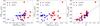 |
Fig. 15 Relationship between dust spectra peak equivalent width and stellar mass (left panel), dust luminosity (central panel), and Dale et al. (2014)α parameter (right panel). Filled red squares represent ULIRGs, and filled blue triangles correspond to LIRGs. The most extreme value of EWdust was found for the most distant object in the ADF–S sample (z = 1.23): a quasar HE 0435-5304. The dashed line represents the linear fit to the data. In the α–EWdust relation (right panel) 2σ uncertainties for the fitted line (Eq. (7)) were added (solid gray lines). |
Based on the best fitted model found by CIGALE, we calculated artificial half equivalent widths of the dust peaks of the spectra (EWdust). We defined this value as the difference between the wavelength for the maximal value of the dust peak (λmax) and the 24 μm (λ24 μm) for the rest-frame spectra multiplied by two: 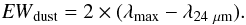 (6)We checked how the physical properties of LIRGs and ULIRGs are related to the width of the dust emission peak. Our results show that stellar mass and dust luminosity increase with the increasing EWdust (Fig. 15), but the scatter is too large to propose any strict relations. The same plot includes the α parameter from Dale et al. (2014) as a function of EWdust. EWdust correlates very well with Dale et al. (2014)α parameter. Thus, the α–EWdust relation can be written as:
  (7)where 0.3 uncertainty corresponds to the 2σ level (more than 95% of LIRGs and ULIRGs are within that distance from the line determined by the Eq. (7)). This implies that the wider the dust emission peak of the spectrum, the more quiescent a galaxy is. The notable exception is, again, the most distant galaxy in the sample (quasar HE 0435-5304), as the SFR for this object is equal to 2834.36 ± 978.20 [M⊙ yr-1], and α = 2.83 ± 0.59.
We also measured the distribution of the λmax parameter itself (Fig. 6). We found that the majority of LIRGs and ULIRGs are cold (i.e., characterized by the IR peak at wavelengths longer than 90 μm). This finding is in agreement with Symeonidis et al. (2011).
5.7. Dust temperatures and dust mass for ADF–S LIRGs and ULIRGs
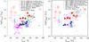 |
Fig. 16 Relation of dust temperature versus dust luminosity for local (left panel), and higher redshift LIRGs and ULIRGs (right panel). Red squares represent ULIRGs, and blue triangles – LIRGs from the ADF–S sample (empty symbols represent object without Herschel data). Left panel: open magenta circles denote Pereira-Santaella et al. (2015) sample of LIRGs, open green triangles stand for Symeonidis et al. (2013), black “x-s” – U et al. (2012) sample of LIRGs and ULIRGs, and open cyan squares – Clements et al. (2010) sample of ULIRGs at redshift range z < 1. Right panel: open magenta traingles represent Santos et al. (2015) sample of LIRGs and ULIRGs, black “x-s” – LIRGs and ULIRGs from da Cunha et al. (2015), and green open circles represent Yan et al. (2014) ULIRGs sample. The errorbars of da Cunha et al. (2015) data were not shown since they are very large and make the plot unreadable. |
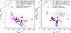 |
Fig. 17 Dust luminosity versus dust mass for local (left panel) and hight redshift LIRGs and ULIRGs (right panel). Red squares represent LIRGs, while blue triangles – ULIRGs from the ADF–S sample (empty symbols present object without Herschel data). Left panel: black crosses represent LIRGs and ULIRGs from U et al. (2012), and open pink circles correspond to the Pereira-Santaella et al. (2015) sample of LIRGs. Right panel: open green circles represent Yan et al. (2014) ULIRGs, black “x-s” – LIRGs and ULIRGs from da Cunha et al. (2015), open pink triangles represent Podigachoski et al. (2015) sample of LIRGs and ULIRGs, and open cyan squares – Clements et al. (2010) sample of ULIRGs. The errorbars of da Cunha et al. (2015) data were not shown since they are very large and make the plot unreadable. |
We used the Casey (2012) model, and the CMCIRSED pipeline, in order to obtain the independent identification of LIRGs and ULIRGs from the ADF–S sample, and, for objects characterized by log (Ldust) > = 11 [L⊙] by both methods, to calculate Tdust and Mdust. Figures 16, and 17 show the dust luminosity/dust temperature, and the dust temperature/dust mass relationships for 25 objects identified as LIRGs and ULIRGs both by CIGALE, and CMCIRSED, and the corresponding measurements from the literature. All ADF–S LIRGs and ULIRGs are marked by red squares (ULIRGs) and blue traingles (LIRGs); empty symbols represent objects without Herschel counterparts.
Our first conclusion is that the power-law + graybody fitting for objects without measurements at wavelengths longer than 160 μm (without Herschel/SPIRE data) results in suspiciously low temperature values (lower than 20 K), and thus should be treated as unreliable. The lack of long-wavelength data forbids a proper estimation of the dust peak in the spectrum (e.g., U et al. 2012). This might be caused by the fact that the SED-fitting in such a case is performed only for radiation emitted by the large dust grains (Li 2005), and not all the dust located in a galaxy. As the CMCIRSED can be applied to the infrared data only, we decided to focus on the LIRGs and ULIRGs with both AKARI and Herschel/SPIRE measurements (filled markers), to avoid possible underestimations of the dust temperature. Unfortunately, only five ULIRGs and seven LIRGs fulfill this condition, and thus our sample is reduced by ~60%. Nevertheless to estimate the Tdust−Ldust relation we prefer to use the best quality data (which are not affected by possible bias caused by the incomplete SED).
We compared our results with the known samples of objects located in the similar redshift range (z< 1):
-
U et al. (2012), who used theCMCIRSED model to calculate Tdust, and Mdust values.
-
Symeonidis et al. (2011, 2013) who presented the Herschel sample with Tdust estimated from the graybody emission. The sample consists of 1159 sources: LIRGs and ULIRGs along with normal galaxies, at redshift range 0.1 <z< 2.0.
-
Pereira-Santaella et al. (2015): here Tdust was calculated by fitting the graybody emission, and Mdust was estimated using a power-law function.
-
Clements et al. (2010) sample of local ULIRGs, detected at 850 μ. The temperature used for our comparison was calculated based on the standard modified blackbody fit to SCUBA 850 μm fluxes, and IRAS 60, 100 μm and 450 μm (SCUBA) fluxes where available.
To compare our galaxies with more distant onces, we have also used samples presented by:
-
Podigachoski et al. (2015), whopresented a sample of high-redshift (z> 1) radio-loud AGNs from theRevised Third Cambridge Catalogue of radio sources; the valuesof Tdust were estimated based on the gray-body emission, and Mdust wascalculated in the same way as in theCMCIRSED model.
-
Yan et al. (2014); (redshifts between one and two) Tdust was based on the Siebenmorgen & Krügel (2007) templates, and the stellar mass was computed in the same way as the CMCIRSED model.
-
Santos et al. (2015); z ~ 1.58, Tdust was calculated by the graybody emission function fitting.
-
da Cunha et al. (2015); zmedian = 2.83, Tdust and Mdust were calculated by MAGPHYS model (da Cunha et al. 2010, 2015).
Both local and high redshift samples used for comparison were selected so that they were based on a similar sample selection (IR bands) and an analogous method of estimation of the dust mass and temperature as for the ADF–S data.
5.7.1. Luminosity/temperature relation
We find that the dust temperature increases with the total infrared luminosity, and the relation is similar for ULIRGs and LIRGs (Fig. 16). For the local Universe we compared our results with samples presented by U et al. (2012), Symeonidis et al. (2013), Pereira-Santaella et al. (2011), and Clements et al. (2010) (Fig. 16, left panel). According to Symeonidis et al. (2013), the dust temperature of ULIRGs and LIRGs increases with dust luminosity. The relation found by Symeonidis et al. (2013) is steeper than the Tdust versus Ldust relation for ADF–S, U et al. (2012), and Clements et al. (2010) samples, however in all cases the increase of dust temperature with dust mass is very weak or even insignificant. As Symeonidis et al. (2013) suggested, the temperature-mass relation is shaped by the dust mass, and not the increase in the dust heating. This theory can be supported by the distribution of an α parameter (Fig. 11) for the Dale et al. (2014) templates for LIRG and ULIRG samples. The distribution of the increasing global heating index α is very similar, and the difference between mean values of α between LIRGs and ULIRGs (Table 2) is not significant. At the same time, the α distribution for normal galaxies is significantly different.
The dust luminosity/dust temperature relation for higher z is shown in the right panel of Fig. 16. Here we present a comparison of ADF–S Tdust versus Ldust relation with LIRGs and ULIRGs from Yan et al. (2014), Santos et al. (2015), and da Cunha et al. (2015). It is clearly visible that the shape of the relation is preserved for higher redshifts. We conclude that LIRGs and ULIRGs in the local Universe are usually colder than similar objects at higher redshift. Our conclusion is in agreement with findings presented by Symeonidis et al. (2013), who claims that, in general, the temperature of LIRGs and ULIRGs is approximately constant, and the dust temperature is related to the dust mass. This finding that LIRGs and ULIRGs with low dust mass are found only in the local Universe might be a selection effect.
5.7.2. Dust mass/temperature relation
We tested whether or not our conclusions presented above are confirmed by the Tdust versus Mdust relation (Fig. 17), and show this relation for the ADF–S sample in comparison with other local samples of LIRGs and ULIRGs (U et al. 2012; Pereira-Santaella et al. 2015; Clements et al. 2010, as for these samples, the dust mass and the dust temperature are available). We found that more dusty galaxies have lower dust temperature. In other words, the dust temperature increases with decreasing dust mass. This relation holds most significantly for LIRGs. For ULIRGs the Tdust versus Mdust relation is not that obvious, and both ADF–S and Clements et al. (2010) samples show no dependence on the dust mass. Comparing our data to Yan et al. (2014), Podigachoski et al. (2015), and da Cunha et al. (2015) samples at redshift >1, we find that this behavior is preserved for higher redshift. However, the Tdust versus Mdust relation for both local and z> 1 samples shows a more general relation: dust mass and dust temperature increasing with redshift, but we claim that this relation might be caused by a selection effect where for higher redshifts we can detect only IR bright galaxies.
6. Fractional contribution of AGN MIR emission and types of AGNs
As the role of AGNs in LIRGs and ULIRGs is still not entirely clear, one of the main aims of our analysis was to estimate the AGN contribution to the LIRGs’ and ULIRGs’ infrared emission and which types of AGNs are related to LIRGs’ and ULIRGs’ activity. As we have shown, the ADF–S LIRGs and ULIRGs are comparable to LIRGs and ULIRGs selected by other authors in IR wavelengths, and our sample can be representative for the whole population.
We have derived the fractional contribution of the AGN MIR emission for Fritz et al. (2006) templates, which are built on two components: (1) point-like isotropic emission of the central source; and (2) radiation from dust with a toroidal geometry in the vicinity of the central engine. The AGN emission is absorbed by the toroidal obscurer and re-emitted at 1–1000 μm wavelengths or scattered by the same obscurer. The Fritz et al. (2006) model describes different types of AGNs: Type 1, Type 2, and intermediate states. We perform SED fitting with a set of parameters of Fritz et al. (2006) models as described by Ciesla et al. (2015). We decided to use the same input list as Ciesla et al. (2015), checking all possible biases, and the influence of input parameters on the final physical properties using the mock catalog.
Figure 18 presents a fractional contribution of AGNs to LIRGs and ULIRGs. We find that for 25 LIRGs and ULIRGs (more than 64% of the sample) the AGN contribution is higher than 10%. In general, ULIRGs are characterized by a higher fraction of AGNs than are LIRGs. Moreover, the AGNfrac. parameter increases with dust luminosity. Our findings are consistent with results presented by Lin et al. (2016) for LIRGs and ULIRGs selected at 70 μm. The majority of ADF–S ULIRGs show an AGN contribution to the MIR luminosity higher than 20%. Based on Ciesla et al. (2015), the fractional contribution of AGN emission to the Ldust constrained by CIGALE is almost always overestimated for a low fraction of Type 1 AGNs (<10%), and underestimated for AGNfrac.> 20% for Type 1 and intermediate types of AGNs. As most LIRGs and ULIRGs are characterized by AGNfrac.> 10% we conclude that the real contribution might be underestimated, and thus the values we have obtained may be treated as lower limits.
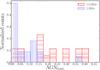 |
Fig. 18 Fractional contribution of AGN to the MIR emission of LIRGs and ULIRGs. The horizontal striped red histogram represents ULIRGs while the vertical striped blue histogram corresponds to LIRGs. |
Mean, median, and maximal values of the AGN-fraction for the ADF–S LIRGs and ULIRGs.
Previous studies of local LIRGs and ULIRGs also found a similar contribution of AGNs to ULIRGs (~20%; Giovannoli et al. 2011; Fiorenza et al. 2014; Pereira-Santaella et al. 2011, Petric et al. 2011; Farrah et al. 2007). The mean and median values of the AGN fraction for LIRGs and ULIRGs in our sample are presented in Table 3. The median fraction of AGNs in ULIRGs is 19% in accordance with previous studies. The AGN contribution to dust luminosity for LIRGs is slightly lower (~13%). The mean and median values of AGNfrac. for LIRGs and ULIRGs are very similar, and their uncertainties are not high.
The maximum value of an AGN fraction among ULIRGs (41%) was obtained for galaxy APMUKS(BJ) B043219.97-543942.2 (IDADFS = 59), with photometric redshift equal to 0.50. Among the LIRGs, we found a maximal AGN contribution (35 ± 4%) for the Syfert galaxy RBS 0567 (IDADFS = 610) with a known spectroscopic redshift equal to 0.24.
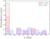 |
Fig. 19 Angle with respect to the line of sight (ψ) for the ADF–S LIRGs and ULIRGs sample. The striped red histogram represents ULIRGs while the vertical striped blue histogram represents LIRGs. |
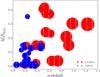 |
Fig. 20 Relationship between redshift and fractional contribution of AGN MIR emission for ULIRGs and LIRGs from the ADF–S sample. Filled red squares represent ULIRGs, while filled blue triangles represent LIRGs. The radii of circles correspond to the log(SFR) values for each galaxy (we used this as a scaling factor), that is, the larger the circle, the higher the measured SFR of the galaxy. |
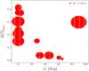 |
Fig. 21 Relationship between the torus angle with respect to the line of sight (ψ) and the fractional contribution of AGN MIR emission for ULIRGs from the ADF–S sample. Radii of circles correspond to the redshift for each galaxy (used as a scaling factor; larger circles correspond to higher redshifts). One outlier, the galaxy with torus angle equal to 89°, is the most distant galaxy in our sample with zspec = 1.23 (a detailed discussion of this specific quasar can be found in Sect. 4.1.3). |
Based on results obtained from the AGN component, we conclude that we can distinguish different types of AGN components for LIRGs and ULIRGs. Figure 19 presents the distribution of ψ for ADF–S LIRGs and ULIRGs. It shows that LIRGs consist of both Type 1 and Type 2 AGNs, as well as intermediate types, whereas for ULIRGs, a majority of fractional contribution of AGN emission originates from Type 2 AGNs. Veilleux et al. (1995) and Kim et al. (1998) showed that the percentage of Type 1 AGNs increases with increasing infrared luminosity, and they found no contribution to the MIR luminosity from the Type 1 AGNs up to log (Ldust/L⊙) < 12.3. Their results are not in contradiction with our findings: Type 1 AGNs have, in general, a small influence on the MIR luminosity for the ADF-S LIRG sample (mean fractional contribution of Type 1 AGN MIR emission for ADF–S LIRG sample is equal to 9 ± 3%).
Our result shows that 70% of ADF–S ULIRGs contain Type 2 AGNs, and for them, the mean fractional contribution of AGN to the MIR emission is equal to 26 ± 5% and the obtained value is only slightly lower than the AGN contribution for ~z< 0.3 ULIRGs observed by Spitzer Infrared Spectrograph, and analyzed by Veilleux et al. (2009) for which the total AGN contribution equals 35–40%. This suggests that Type 1 AGNs make only a small contribution to the MIR emission for galaxies with Ldust> 1012 [L⊙], and the high luminosity of the dust part of the spectra is related to their star-forming activity. Figure 21 shows the relationship between the torus angle with respect to the line of sight and the fractional contribution of AGNs to the MIR emission of ULIRGs. The general trend suggests that ULIRGs containing Type 2 AGNs are characterized by a higher AGN contribution. The one outstanding object with high AGNfrac and ψ ~ 90 is the HLIRG and a known quasar with log (Ldust) = 13.12 ± 0.29 [L⊙].
Our measurements indicate that Type 2 and intermediate types of AGNs occur more often in the ADF–S ULIRGs than Type 1 AGNs. It has already been shown by other authors (e.g., Lonsdale et al. 2006) that warm ULIRGs tend to have optical spectral features indicating the presence of Type 1 AGNs while cool ULIRGs have characteristics of starburst or Type 2 AGNs. Cool MIR colors (the galaxy displaying cool MIR color has a ratio between fluxes measured at 25 and 60 μm lower than 0.2; as we did not use IRAS bands for our analysis, we have measured the ratio between the modeled fluxes) and positions of dust peaks of the spectra located at wavelengths longer than 90 μm (Fig. 6) indicate that almost all the ADF-S ULIRGs are cool, and associating them with Type 2 AGNs is indeed consistent with previous observations.
The question emerges as to why it might be that cool ULIRGs have a higher chance of containing an edge–on AGN than a face–on type AGN. If we make an assumption that ULIRGs’ IR emission is isotropic; such a finding could undermine the unification theory of AGNs according to which Seyfert 1 and 2 galaxies are the same kind of objects, surrounded by an optically thick dust torus but viewed from different angles (Antonucci 1993). Indeed, such an explanation of the observed preference of different kinds of ULIRGs to host different types of AGNs was suggested by Veilleux et al. (1997) and Lee et al. (2011), for example.
A much more likely explanation may be the geometrical contribution from the host galaxy, as the host galaxy orientation may add some bias. In particular, a non-isotropic dust distribution resulting in the (cold) dust column density along the line of sight being higher in the case of the egde–on objects might increase their infrared luminosity resulting in the detection of an object as an ULIRG. From a broader perspective, it might lead to a unification scenario for LIRGs and ULIRGs, in which seeing a galaxy as a cold/warm ULIRG or LIRG could be related to the geometry of the object rather than, or together with, its physical properties. However, confirming or rejecting such a hypothesis requires further observations of both ULIRGs’ host galaxies and their central AGNs.
7. Conclusions
We analyzed the physical properties of a sample of 178 infrared-selected galaxies detected at 90 μm. For our analysis we used one of the deep AKARI surveys, ADF–S, and the catalogs published by Małek et al. (2010) and Małek et al. (2013), completed by spectroscopic redshifts and Herschel/SPIRE data.
The CIGALE v.0.5 (Noll et al. 2009; Burgarella et al., in prep.) program for fitting spectral energy distribution was used to estimate basic physical properties of the ADF-S sources: stellar mass, dust luminosity, SFR, dust heating intensity, AGN fraction of MIR emission, and the AGN’s viewing angle with respect to the line of sight. SEDs were fitted for all 78 galaxies, and for 69 sources (20 with spectroscopic and 49 with photometric redshifts) the quality of the fits was satisfactory and the obtained physical parameters were deemed reliable.
Additionally, we used a graybody + power law CMCIRSED SED modeling code for the final sample of 69 ADF–S galaxies, to obtain independent measurements of dust luminosity, and to calculate dust mass and dust temperature for LIRGs and ULIRGs. With the use of CMCIRSED, we find 13 LIRGs and 12 ULIRGs (this discrepancy between the results given by both codes might be expounded as the lack of Herschel/SPIRE data for some galaxies, while very far infrared data are crucial for a code based on the FIR data only). Thus, galaxies with log (Ldust) ≥ 11 [L⊙] compose 25% of our sample.
Based on the UV-FIR and FIR only SED fitting, we find that:
-
1.
The ADF–S sample mainly consists of galaxies active in star formation.
-
2.
Using CIGALE, among 69 ADF–S galaxies, we find 17 ULIRGs and 22 LIRGs, spanning over the redshift range 0.06 <z< 1.2. The majority of them have the IR peak placed at wavelengths longer than 90 μm (so called cold LIRGs and ULIRGs, Symeonidis et al. 2011),
-
3.
Galaxies bright in the FIR are relatively massive (mean log (Mstars) computed for ULIRGs and LIRGs, and galaxies with log (Ldust) < 11 [L⊙] is equal to 11.51 ± 0.37, 10.90 ± 0.56, and 10.03 ± 0.50 [M⊙], respectively). Our results are consistent with stellar masses calculated for LIRGs and ULIRGs located at similar redshifts, selected from IR surveys (U et al. 2012; Pereira-Santaella et al. 2011; Giovannoli et al. 2011; Melbourne et al. 2008; Santos et al. 2015; da Cunha et al. 2015; Rothberg et al. 2013).
-
4.
The mean log(SFR) for ULIRGs, LIRGs, and the rest of ADF–S galaxies is equal to 2.53 ± 0.39, 1.48 ± 0.24, and 0.47 ± 0.21 [M⊙ yr-1], respectively, and these results are consistent with the Kennicutt (1998) relation. Our results are consistent with those presented in the literature, that is, Santos et al. (2015), Podigachoski et al. (2015), da Cunha et al. (2015), and Howell et al. (2010). The SFR increases with Ldust in the same way as normal galaxies, LIRGs, and ULIRGs.
-
5.
ADF–S “normal” star-forming galaxies follow the general SFR–Mstar correlation as defined by Noeske et al. (2007). However, the majority of ADF–S LIRGs and ULIRGs are located above the correlation line and they are shifted toward higher SFR.
-
6.
We calculated the specific SFR and found that SSFR decreases with increasing stellar mass, with a similar slope as the SSFR−Mstar relation for the whole ADF–S sample (−0.72, −0.92, and −0.75, for ULIRGs, LIRGs, and normal galaxies, respectively).
-
7.
We calculated the artificial equivalent width of the dust component, defined as EWdust = 2 × (λmax−λ24μ m). We find that the stellar mass, the dust luminosity, and the α parameter from Dale et al. (2014) for LIRGs and ULIRGs increase with increasing width of dust component, and find a steep correlation between α and EWdust with a slope equal to 0.6 ± 0.3 + (0.0042 ×EWdust).
A dust temperature/mass analysis was performed for LIRGs and ULIRGs selected by both fitting methods (CIGALE and CMCIRSED). As the visual inspection of CMCIRSED SEDs shows a difference in quality of the fitted spectra between galaxies with and without Herschel/SPIRE data (lack of measurements after the peak of the dust emission), we based this part of the analysis on the 12 LIRGs and ULIRGs with AKARI–Herschel data and found that the Tdust/Ldust relationship for ADF–S LIRGs and ULIRGs agrees with the literature. The relation is rather flat, and flatter than the same relation estimated by Symeonidis et al. (2013). As was suggested by Symeonidis et al. (2013), this relation is shaped by the dust mass, and not the increase in dust heating.
Based on the UV–FIR SED fitting method, we conclude that the median fractional contribution of AGN MIR emission for ADF–S ULIRGs is 19%. The AGN contribution in the dust luminosity of LIRGs is slightly lower, and equal to 13%. We find that the ADF–S LIRG sample consists both of Type 1, and Type 2 AGNs, as well as intermediate types. At the same time, for ULIRGs selected at 90 μm AKARI band, the majority of fractional contribution of AGN emission originates from Type 2 AGNs.
σMED = 1.48 × | Δz/ (1 + zspectr) |.
Model available on-line at http://herschel.uci.edu/cmcasey/sedfitting.html
Acknowledgments
We thank the anonymous referee for useful comments and suggestions. This work is based on observations with AKARI, a JAXA project with the participation of ESA. Research was conducted in the scope of the HECOLS International Associated Laboratory. This research has made use of the SIMBAD database, operated at CDS, Strasbourg, France, the NASA/IPAC Extragalactic Database (NED), which is operated by the Jet Propulsion Laboratory, and the California Institute of Technology, under contract with the National Aeronautics and Space Administration. This research has made use of the NASA/IPAC Infrared Science Archive, which is operated by the Jet Propulsion Laboratory, California Institute of Technology, under contract with the National Aeronautics and Space Administration. This research has made use of data from HerMES project (http://hermes.sussex.ac.uk/). HerMES is a Herschel Key Programme utilising Guaranteed Time from the SPIRE instrument team, ESAC scientists and a mission scientist. The HerMES data was accessed through the Herschel Database in Marseille (HeDaM – http://hedam.lam.fr) operated by CeSAM and hosted by the Laboratoire d’Astrophysique de Marseille. This work have been supported by the Polish National Science Centre (grants UMO-2012/07/B/ST9/04425 and UMO-2013/09/D/ST9/04030), and the European Associated Laboratory Astrophysics Poland-France HECOLS. M.M. acknowledges support from NASA grants NNX08AU59G and NNX09AM45G for analysis of GALEX data in the AKARI Deep Fields. T.T.T. has been supported by the Grant-in- Aid for the Scientific Research Fund (24111707), and by the Strategic Young Researches Overseas Visits Program for Accelerating Brain Circulation commissioned by the Ministry of Education, Culture, Sports, Science and Technology (MEXT) of Japan.
References
- Abell, G. O., Corwin, H. G. J., & Olowin, R. P. 1989, ApJS, 70, 1 [NASA ADS] [CrossRef] [EDP Sciences] [Google Scholar]
- Alonso-Herrero, A., Pereira-Santaella, M., Rieke, G. H., & Rigopoulou, D. 2012, ApJ, 744, 2 [NASA ADS] [CrossRef] [Google Scholar]
- Antonucci, R. 1993, ARA&A, 31, 473 [Google Scholar]
- Armus, L., Mazzarella, J. M., Evans, A. S., et al. 2009, PASP, 121, 559 [NASA ADS] [CrossRef] [Google Scholar]
- Arnouts, S., Cristiani, S., Moscardini, L., et al. 1999, MNRAS, 310, 540 [NASA ADS] [CrossRef] [Google Scholar]
- Bolzonella, M., Miralles, J.-M., & Pelló, R. 2000, A&A, 363, 476 [NASA ADS] [Google Scholar]
- Boquien, M., Buat, V., Boselli, A., et al. 2012, A&A, 539, A145 [NASA ADS] [CrossRef] [EDP Sciences] [Google Scholar]
- Brinchmann, J., Charlot, S., White, S. D. M., et al. 2004, MNRAS, 351, 1151 [NASA ADS] [CrossRef] [Google Scholar]
- Bruzual, G., & Charlot, S. 2003, MNRAS, 344, 1000 [NASA ADS] [CrossRef] [Google Scholar]
- Buat, V., Takeuchi, T. T., Iglesias-Páramo, J., et al. 2007, ApJS, 173, 404 [NASA ADS] [CrossRef] [Google Scholar]
- Buat, V., Giovannoli, E., Takeuchi, T. T., et al. 2011, A&A, 529, A22 [NASA ADS] [CrossRef] [EDP Sciences] [Google Scholar]
- Buat, V., Heinis, S., Boquien, M., et al. 2014, A&A, 561, A39 [NASA ADS] [CrossRef] [EDP Sciences] [Google Scholar]
- Buat, V., Oi, N., Heinis, S., et al. 2015, A&A, 577, A141 [NASA ADS] [CrossRef] [EDP Sciences] [Google Scholar]
- Calzetti, D., Armus, L., Bohlin, R. C., et al. 2000, ApJ, 533, 682 [NASA ADS] [CrossRef] [Google Scholar]
- Calzetti, D., Kennicutt, R. C., Engelbracht, C. W., et al. 2007, ApJ, 666, 870 [NASA ADS] [CrossRef] [Google Scholar]
- Caputi, K. I., Lagache, G., Yan, L., et al. 2007, ApJ, 660, 97 [NASA ADS] [CrossRef] [Google Scholar]
- Carpineti, A., Kaviraj, S., Hyde, A. K., et al. 2015, A&A, 577, A119 [NASA ADS] [CrossRef] [EDP Sciences] [Google Scholar]
- Casey, C. M. 2012, MNRAS, 425, 3094 [Google Scholar]
- Castellano, M., Amorín, R., Merlin, E., et al. 2016, A&A, 590, A31 [NASA ADS] [CrossRef] [EDP Sciences] [Google Scholar]
- Chary, R., & Elbaz, D. 2001, ApJ, 556, 562 [NASA ADS] [CrossRef] [Google Scholar]
- Chevallard, J., Charlot, S., Wandelt, B., & Wild, V. 2013, MNRAS, 432, 2061 [NASA ADS] [CrossRef] [Google Scholar]
- Ciesla, L., Charmandaris, V., Georgakakis, A., et al. 2015, A&A, 576, A10 [NASA ADS] [CrossRef] [EDP Sciences] [Google Scholar]
- Clements, D. L., Sutherland, W. J., Saunders, W., et al. 1996, MNRAS, 279, 459 [NASA ADS] [CrossRef] [Google Scholar]
- Clements, D. L., Dunne, L., & Eales, S. 2010, MNRAS, 403, 274 [NASA ADS] [CrossRef] [Google Scholar]
- Cowie, L. L., Songaila, A., Hu, E. M., & Cohen, J. G. 1996, AJ, 112, 839 [Google Scholar]
- da Cunha, E., Charmandaris, V., Díaz-Santos, T., et al. 2010, A&A, 523, A78 [NASA ADS] [CrossRef] [EDP Sciences] [Google Scholar]
- da Cunha, E., Walter, F., Smail, I. R., et al. 2015, ApJ, 806, 110 [NASA ADS] [CrossRef] [Google Scholar]
- Dahlen, T., Mobasher, B., Faber, S. M., et al. 2013, ApJ, 775, 93 [Google Scholar]
- Dale, D. A., & Helou, G. 2002, ApJ, 576, 159 [NASA ADS] [CrossRef] [Google Scholar]
- Dale, D. A., Helou, G., Contursi, A., Silbermann, N. A., & Kolhatkar, S. 2001, ApJ, 549, 215 [NASA ADS] [CrossRef] [Google Scholar]
- Dale, D. A., Bendo, G. J., Engelbracht, C. W., et al. 2005, ApJ, 633, 857 [NASA ADS] [CrossRef] [Google Scholar]
- Dale, D. A., Gil de Paz, A., Gordon, K. D., et al. 2007, ApJ, 655, 863 [NASA ADS] [CrossRef] [Google Scholar]
- Dale, D. A., Helou, G., Magdis, G. E., et al. 2014, ApJ, 784, 83 [NASA ADS] [CrossRef] [Google Scholar]
- Draine, B. T., & Li, A. 2007, ApJ, 657, 810 [NASA ADS] [CrossRef] [Google Scholar]
- Dressler, A. 1980a, ApJS, 42, 565 [NASA ADS] [CrossRef] [Google Scholar]
- Dressler, A. 1980b, ApJ, 236, 351 [NASA ADS] [CrossRef] [Google Scholar]
- Elbaz, D., Daddi, E., Le Borgne, D., et al. 2007, A&A, 468, 33 [NASA ADS] [CrossRef] [EDP Sciences] [Google Scholar]
- Erb, D. K., Steidel, C. C., Shapley, A. E., et al. 2006, ApJ, 646, 107 [NASA ADS] [CrossRef] [Google Scholar]
- Farrah, D., Bernard-Salas, J., Spoon, H. W. W., et al. 2007, ApJ, 667, 149 [NASA ADS] [CrossRef] [Google Scholar]
- Feltre, A., Hatziminaoglou, E., Fritz, J., & Franceschini, A. 2012, MNRAS, 426, 120 [NASA ADS] [CrossRef] [Google Scholar]
- Fiorenza, S. L., Takeuchi, T. T., Małek, K. E., & Liu, C. T. 2014, ApJ, 784, 140 [NASA ADS] [CrossRef] [Google Scholar]
- Fisher, K. B., Huchra, J. P., Strauss, M. A., et al. 1995, ApJS, 100, 69 [NASA ADS] [CrossRef] [Google Scholar]
- Fritz, J., Franceschini, A., & Hatziminaoglou, E. 2006, MNRAS, 366, 767 [Google Scholar]
- Giovannoli, E., Buat, V., Noll, S., Burgarella, D., & Magnelli, B. 2011, A&A, 525, A150 [NASA ADS] [CrossRef] [EDP Sciences] [Google Scholar]
- Goto, T., Takagi, T., Matsuhara, H., et al. 2010, A&A, 514, A6 [NASA ADS] [CrossRef] [EDP Sciences] [Google Scholar]
- Griffin, M. J., Abergel, A., Abreu, A., et al. 2010, A&A, 518, L3 [Google Scholar]
- Hatziminaoglou, E., Fritz, J., Franceschini, A., et al. 2008, MNRAS, 386, 1252 [NASA ADS] [CrossRef] [Google Scholar]
- Hatziminaoglou, E., Fritz, J., & Jarrett, T. H. 2009, MNRAS, 399, 1206 [NASA ADS] [CrossRef] [Google Scholar]
- Heinis, S., Gezari, S., Kumar, S., et al. 2016, ApJ, 826, 62 [NASA ADS] [CrossRef] [Google Scholar]
- Houck, J. R., Schneider, D. P., Danielson, G. E., et al. 1985, ApJ, 290, L5 [NASA ADS] [CrossRef] [Google Scholar]
- Howell, J. H., Armus, L., Mazzarella, J. M., et al. 2010, ApJ, 715, 572 [NASA ADS] [CrossRef] [Google Scholar]
- Hung, C.-L., Sanders, D. B., Casey, C. M., et al. 2014, ApJ, 791, 63 [Google Scholar]
- Iglesias-Páramo, J., Buat, V., Hernández-Fernández, J., et al. 2007, ApJ, 670, 279 [NASA ADS] [CrossRef] [Google Scholar]
- Ilbert, O., Arnouts, S., McCracken, H. J., et al. 2006, A&A, 457, 841 [NASA ADS] [CrossRef] [EDP Sciences] [Google Scholar]
- Ilbert, O., McCracken, H. J., Le Fèvre, O., et al. 2013, A&A, 556, A55 [NASA ADS] [CrossRef] [EDP Sciences] [Google Scholar]
- Jones, D. H., Saunders, W., Colles, M., et al. 2004, MNRAS, 355, 747 [NASA ADS] [CrossRef] [Google Scholar]
- Jones, D. H., Read, M. A., Saunders, W., et al. 2009, MNRAS, 399, 683 [NASA ADS] [CrossRef] [Google Scholar]
- Kawada, M., Baba, H., Barthel, P. D., et al. 2007, PASJ, 59, 389 [Google Scholar]
- Keeney, B. A., Stocke, J. T., Rosenberg, J. L., et al. 2013, ApJ, 765, 27 [NASA ADS] [CrossRef] [Google Scholar]
- Kennicutt, Jr., R. C. 1998, ARA&A, 36, 189 [Google Scholar]
- Kim, D.-C. 1995, Ph.D. Thesis, University of Hawaii [Google Scholar]
- Kim, D.-C., & Sanders, D. B. 1998, ApJS, 119, 41 [NASA ADS] [CrossRef] [Google Scholar]
- Kim, D.-C., Veilleux, S., & Sanders, D. B. 1998, ApJ, 508, 627 [NASA ADS] [CrossRef] [Google Scholar]
- Kroupa, P. 2001, MNRAS, 322, 231 [NASA ADS] [CrossRef] [Google Scholar]
- Le Floc’h, E., Papovich, C., Dole, H., et al. 2005, ApJ, 632, 169 [NASA ADS] [CrossRef] [Google Scholar]
- Lee, J. C., Hwang, H. S., Lee, M. G., Kim, M., & Kim, S. C. 2011, MNRAS, 414, 702 [NASA ADS] [CrossRef] [Google Scholar]
- Lee, S.-K., Idzi, R., Ferguson, H. C., et al. 2009, ApJS, 184, 100 [NASA ADS] [CrossRef] [Google Scholar]
- Li, A. 2005, ArXiv e-prints [arXiv:astro-ph/0503571] [Google Scholar]
- Lin, M.-Y., Hashimoto, Y., & Foucaud, S. 2016, MNRAS, 456, 2735 [NASA ADS] [CrossRef] [Google Scholar]
- Lonsdale, C. J., Farrah, D., & Smith, H. E. 2006, Ultraluminous Infrared Galaxies, ed. J. W. Mason (UK: Springer Praxis Book), 285 [Google Scholar]
- Magnelli, B., Elbaz, D., Chary, R. R., et al. 2009, A&A, 496, 57 [NASA ADS] [CrossRef] [EDP Sciences] [Google Scholar]
- Małek, K., Pollo, A., Takeuchi, T. T., et al. 2010, A&A, 514, A11 [NASA ADS] [CrossRef] [EDP Sciences] [Google Scholar]
- Małek, K., Pollo, A., Takeuchi, T. T., et al. 2013, Earth, Planets, and Space, 65, 1101 [Google Scholar]
- Małek, K., Pollo, A., Takeuchi, T. T., et al. 2014, A&A, 562, A15 [NASA ADS] [CrossRef] [EDP Sciences] [Google Scholar]
- Maraston, C. 2005, MNRAS, 362, 799 [NASA ADS] [CrossRef] [Google Scholar]
- Maraston, C., Nieves Colmenárez, L., Bender, R., & Thomas, D. 2009, A&A, 493, 425 [NASA ADS] [CrossRef] [EDP Sciences] [Google Scholar]
- Melbourne, J., Ammons, M., Wright, S. A., et al. 2008, AJ, 135, 1207 [NASA ADS] [CrossRef] [Google Scholar]
- Moutard, T., Arnouts, S., Ilbert, O., et al. 2016, A&A, 590, A102 [NASA ADS] [CrossRef] [EDP Sciences] [Google Scholar]
- Murakami, H., Baba, H., Barthel, P., et al. 2007, PASJ, 59, 369 [Google Scholar]
- Murphy, Jr., T. W., Armus, L., Matthews, K., et al. 1996, AJ, 111, 1025 [NASA ADS] [CrossRef] [Google Scholar]
- Nardini, E., Risaliti, G., Salvati, M., et al. 2009, MNRAS, 399, 1373 [NASA ADS] [CrossRef] [Google Scholar]
- Nardini, E., Risaliti, G., Watabe, Y., Salvati, M., & Sani, E. 2010, MNRAS, 405, 2505 [NASA ADS] [Google Scholar]
- Neugebauer, G., Habing, H. J., van Duinen, R., et al. 1984, ApJ, 278, 1 [NASA ADS] [CrossRef] [Google Scholar]
- Noeske, K. G., Weiner, B. J., Faber, S. M., et al. 2007, ApJ, 660, L43 [Google Scholar]
- Noll, S., Burgarella, D., Giovannoli, E., et al. 2009, A&A, 507, 1793 [NASA ADS] [CrossRef] [EDP Sciences] [Google Scholar]
- Oliver, S. J., Bock, J., Altieri, B., et al. 2012, MNRAS, 424, 1614 [NASA ADS] [CrossRef] [EDP Sciences] [Google Scholar]
- Paturel, G., Petit, C., Rousseau, J., & Vauglin, I. 2003, A&A, 405, 1 [NASA ADS] [CrossRef] [EDP Sciences] [Google Scholar]
- Pereira-Santaella, M., Alonso-Herrero, A., Santos-Lleo, M., et al. 2011, A&A, 535, A93 [NASA ADS] [CrossRef] [EDP Sciences] [Google Scholar]
- Pereira-Santaella, M., Alonso-Herrero, A., Colina, L., et al. 2015, A&A, 577, A78 [NASA ADS] [CrossRef] [EDP Sciences] [Google Scholar]
- Pérez-González, P. G., Rieke, G. H., Egami, E., et al. 2005, ApJ, 630, 82 [NASA ADS] [CrossRef] [Google Scholar]
- Petric, A. O., Armus, L., Howell, J., et al. 2011, ApJ, 730, 28 [NASA ADS] [CrossRef] [Google Scholar]
- Podigachoski, P., Barthel, P. D., Haas, M., et al. 2015, A&A, 575, A80 [NASA ADS] [CrossRef] [EDP Sciences] [Google Scholar]
- Rafelski, M., Teplitz, H. I., Gardner, J. P., et al. 2015, AJ, 150, 31 [NASA ADS] [CrossRef] [Google Scholar]
- Rieke, G. H., Young, E. T., Engelbracht, C. W., et al. 2004, ApJS, 154, 25 [NASA ADS] [CrossRef] [Google Scholar]
- Rothberg, B., Fischer, J., Rodrigues, M., & Sanders, D. B. 2013, ApJ, 767, 72 [NASA ADS] [CrossRef] [Google Scholar]
- Salpeter, E. E. 1955, ApJ, 121, 161 [Google Scholar]
- Sanders, D. B., & Mirabel, I. F. 1996, ARA&A, 34, 749 [NASA ADS] [CrossRef] [Google Scholar]
- Sanders, D. B., Soifer, B. T., Elias, J. H., et al. 1988, ApJ, 325, 74 [NASA ADS] [CrossRef] [Google Scholar]
- Sanders, D. B., Mazzarella, J. M., Kim, D.-C., Surace, J. A., & Soifer, B. T. 2003, AJ, 126, 1607 [Google Scholar]
- Santos, J. S., Altieri, B., Valtchanov, I., et al. 2015, MNRAS, 447, L65 [NASA ADS] [CrossRef] [Google Scholar]
- Schweitzer, M., Lutz, D., Sturm, E., et al. 2006, ApJ, 649, 79 [NASA ADS] [CrossRef] [Google Scholar]
- Sedgwick, C., Serjeant, S., Pearson, C., et al. 2011, MNRAS, 416, 1862 [NASA ADS] [CrossRef] [Google Scholar]
- Shirahata, M., Matsuura, S., Hasegawa, S., et al. 2009a, PASJ, 61, 737 [NASA ADS] [CrossRef] [Google Scholar]
- Shirahata, M., Matsuura, S., Kawada, M., et al. 2009b, in AKARI, a light to illuminate the misty Universe, eds. T. Onaka, G. J. White, T. Nakagawa, & I. Yamamura, ASP Conf. Ser., 418, 301 [Google Scholar]
- Siebenmorgen, R., & Krügel, E. 2007, A&A, 461, 445 [NASA ADS] [CrossRef] [EDP Sciences] [Google Scholar]
- Simm, T., Saglia, R., Salvato, M., et al. 2015, A&A, 584, A106 [NASA ADS] [CrossRef] [EDP Sciences] [Google Scholar]
- Skrutskie, M. F., Cutri, R. M., Stiening, R., et al. 2006, AJ, 131, 1163 [NASA ADS] [CrossRef] [Google Scholar]
- Soifer, B. T., Sanders, D. B., Neugebauer, G., et al. 1986, ApJ, 303, L41 [NASA ADS] [CrossRef] [Google Scholar]
- Soifer, B. T., Neugebauer, G., & Houck, J. R. 1987, ARA&A, 25, 187 [NASA ADS] [CrossRef] [Google Scholar]
- Speagle, J. S., Capak, P. L., Eisenstein, D. J., Masters, D. C., & Steinhardt, C. L. 2016, MNRAS, 461, 3432 [NASA ADS] [CrossRef] [Google Scholar]
- Spoon, H. W. W., Marshall, J. A., Houck, J. R., et al. 2007, ApJ, 654, L49 [NASA ADS] [CrossRef] [Google Scholar]
- Symeonidis, M., Page, M. J., & Seymour, N. 2011, MNRAS, 411, 983 [NASA ADS] [CrossRef] [Google Scholar]
- Symeonidis, M., Vaccari, M., Berta, S., et al. 2013, MNRAS, 431, 2317 [NASA ADS] [CrossRef] [Google Scholar]
- Takeuchi, T. T., Buat, V., & Burgarella, D. 2005, A&A, 440, L17 [NASA ADS] [CrossRef] [EDP Sciences] [Google Scholar]
- Thomas, H.-C., Beuermann, K., Reinsch, K., et al. 1998, A&A, 335, 467 [NASA ADS] [Google Scholar]
- U, V., Sanders, D. B., Mazzarella, J. M., et al. 2012, ApJS, 203, 9 [NASA ADS] [CrossRef] [Google Scholar]
- Veilleux, S., Kim, D.-C., Sanders, D. B., Mazzarella, J. M., & Soifer, B. T. 1995, ApJS, 98, 171 [NASA ADS] [CrossRef] [Google Scholar]
- Veilleux, S., Sanders, D. B., & Kim, D.-C. 1997, ApJ, 484, 92 [NASA ADS] [CrossRef] [Google Scholar]
- Veilleux, S., Kim, D.-C., & Sanders, D. B. 2002, ApJS, 143, 315 [NASA ADS] [CrossRef] [Google Scholar]
- Veilleux, S., Rupke, D. S. N., Kim, D.-C., et al. 2009, ApJS, 182, 628 [NASA ADS] [CrossRef] [Google Scholar]
- Véron-Cetty, M.-P., & Véron, P. 2006, A&A, 455, 773 [NASA ADS] [CrossRef] [EDP Sciences] [Google Scholar]
- Walcher, C. J., Lamareille, F., Vergani, D., et al. 2008, A&A, 491, 713 [NASA ADS] [CrossRef] [EDP Sciences] [Google Scholar]
- White, G. J., Hatsukade, B., Pearson, C., et al. 2012, MNRAS, 427, 1830 [NASA ADS] [CrossRef] [Google Scholar]
- Wisotzki, L., Christlieb, N., Bade, N., et al. 2000, A&A, 358, 77 [NASA ADS] [Google Scholar]
- Wright, E. L., Eisenhardt, P. R. M., Mainzer, A. K., et al. 2010, AJ, 140, 1868 [NASA ADS] [CrossRef] [Google Scholar]
- Yan, H., Stefanon, M., Ma, Z., et al. 2014, ApJS, 213, 2 [NASA ADS] [CrossRef] [Google Scholar]
- Yuan, F., Takeuchi, T. T., Buat, V., et al. 2011, PASJ, 63, 1207 [NASA ADS] [Google Scholar]
Appendix A: The influence of the use of photometric redshifts on the final results
To investigate how the photometric redshift uncertainty can affect our results, we performed an additional test: for the final sample of our galaxies we ran the same analysis using redshift values as a redshift ± redshift accuracy, which equals 0.05 (hereafter samplez−0.05 and samplez + 0.05). We calculated the values of dust luminosities, star-formation rates, stellar masses, specific star-formation rates, AGN fractions, torus angles with respect to the lines of sight (ψ), and the slopes of the infrared parts of the spectra (α).
From these two new samples we obtained the same number of HLIRGs (one from samplez−0.05 and samplez + 0.05) as for the original ADF-S sample. Samplez−0.05 gives us 12 ULIRGs, 15 LIRGs, and 38 normal galaxies, while samplez−0.05 gives 18 ULIRGs, 29 LIRGs, and 18 normal galaxies. It is not surprising that with lower redshifts the CIGALE fitter found less ULIRGs and LIRGs, while for higher redshifts we obtained one more ULIRG and seven LIRGs. In general, we observe the trend that bright infrared galaxies at higher redshifts are more often LIRGs than for the lower redshifts, but most of them (~70%) remain in the same luminosity range as that of the original sample. The average physical properties obtained from samplez−0.05 and samplez + 0.05 are consistent with those obtained from the original ADF–S sample and all trends we found remain unchanged. Figure A.1 shows the distribution of physical properties obtained by CIGALE for the ADF–S original sample as well as for samplez−0.05 and samplez + 0.05. For galaxies with redshifts calculated as ADF–S redshifts minus redshift accuracy, the general tendency to lower stellar masses and fainter dust luminosity is visible. All galaxies with log (Ldust) < 9.5 [L⊙], log (Mstar) < 8.8 [M⊙], and log (SFR) < −0.1 have new redshiftsz−0.05~ 0.
The physical properties obtained for both samples are consistent with those presented in the paper (except for galaxies with new redshifts at approximately 0). Most importantly, a general trend between the fractional contribution of AGN MIR emission and the types of AGNs, which was found for ULIRGs and LIRGs from the original ADF-S sample, is preserved, which is shown in Fig. A.2. We conclude that the photometric redshift inaccuracy has a marginal influence on the general trends found in our analysis.
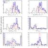 |
Fig. A.1 Distribution of dust luminosity, star-formation rate, stellar mass, fractional contribution of AGN to the MIR emission, AGN’s torus angle with respect to the line of sight (ψ), and IR spectral power-law slope α for an original ADF–S sample (sloping red histogram), and samplez + 0.05 and samplez−0.05 samples (open blue histogram, and dashed black histogram, respectively). |
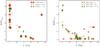 |
Fig. A.2 Relationship between the torus angle with respect to the line of sight (ψ) and the fractional contribution of AGN MIR emission for ULIRGs (left panel) and LIRGs (right panel) for the sample of original ADF-S galaxies (red circles), the ADF-S sample with redshift increased by 0.05 (orange stars) and the ADF-S sample with redshift reduced by value 0.05. |
An example of two rows from the final catalog of 39 LIRGs and ULIRGs selected from the ADF–S sample.
Main physical parameters of the LIRG and ULIRG sample derived based on the CIGALE SED-fitting code (Cols. 3–8) and CMCIRSED code (Cols. 9–12).
All Tables
Main physical parameters for ULIRGs, LIRGs, and galaxies with total infrared luminosity LTIR< 1011L⊙ from the ADF–S sample derived by CIGALE and CMCIRSED.
Mean, median, and maximal values of the AGN-fraction for the ADF–S LIRGs and ULIRGs.
An example of two rows from the final catalog of 39 LIRGs and ULIRGs selected from the ADF–S sample.
Main physical parameters of the LIRG and ULIRG sample derived based on the CIGALE SED-fitting code (Cols. 3–8) and CMCIRSED code (Cols. 9–12).
All Figures
|
Fig. 1 Photometric versus spectroscopic redshifts and redshift accuracy versus spectroscopic redshift for a sample of 84 galaxies (red stars) for which the photometric redshift was calculated by Małek et al. (2014) using the CIGALE tool. Blue squares correspond to the Abell S0463 cluster. The region of CEs, defined as | zspec−zphoto | /(1 + zspec) > 0.15 (Ilbert et al. 2006), is marked by a solid black line. The navy dashed-dotted line corresponds to the zphot = zspec. Shadowed areas represent the redshift range rejected from our analysis. |
| In the text | |
|
Fig. 2 Redshift distribution of the final sample of 78 ADF–S galaxies used for our analysis. |
| In the text | |
|
Fig. 3 Fritz et al. (2006) AGNs’ SEDs used in our analysis. These templates are built based on two optical depth τ9.7 values (1.0 and 6.0), and the extreme values of the angle between the equatorial axis and the line of sight (ψ). The red dotted line represents τ9.7 = 1.0, and ψ = 89.900 [deg]; the green dashed line corresponds to the τ9.7 = 1.0, and ψ = 0.001 [deg]; the black dashed-dotted line to τ9.7 = 6.0, and ψ = 89.900 [deg]; and the blue solid line to τ9.7 = 6.0, and ψ = 0.001 [deg]. |
| In the text | |
|
Fig. 4 Examples of the best fit models (CIGALE SED fitting code). The left-hand side spectrum is a star-forming galaxy, while the spectrum shown on the right-hand side is ULIRG. Observed fluxes are plotted with open blue squares. Filled red circles correspond to the model fluxes. The final model is plotted as a solid black line. The remaining three lines correspond to the stellar, dust, and AGN components. The relative residual fluxes are plotted at the bottom panel of each spectrum. |
| In the text | |
|
Fig. 5 Pearson product-moment correlation coefficient (r) calculated between ADF–S galaxies and the corresponding mock catalog (created from the input values) for dust luminosity, SFR, stellar mass, dust attenuation in V and FUV bands, and α parameter of the model of Dale et al. (2014). The calculated values of r are written above each plot. |
| In the text | |
|
Fig. 6 Number of photometric points used for CIGALE fitting vs. the peak of the dust part of the spectra (λmax for 156 ADF–S objects fitted with χ2< 10). Filled red squares represent ULIRGs, filled blue traingles represent LIRGs, and the gray “x”-s correspond to normal star-forming galaxies. As the λmax corresponds to the dust temperature, we conclude that we do not find any degeneracy with respect to the number of photometric points in the estimation of the peak of the dust part of the spectrum. |
| In the text | |
|
Fig. 7 Normalized redshift distribution of 22 ADF–S LIRGs (vertical striped blue histogram) and 17 ULIRGs (horizontal striped red histogram). |
| In the text | |
|
Fig. 8 χ2 distribution for the ADF-S sample obtained from CMCIRSED code. One galaxy with χ2> 70 is not shown on this histogram. |
| In the text | |
|
Fig. 9 Three examples of the best-fit models by CMCIRSED shown from left to right: ULIRG, LIRG, and a normal galaxy. |
| In the text | |
|
Fig. 10 Distribution of physical properties obtained by CIGALE for the ADF–S galaxies: dust luminosity (Ldust), star formation rate (SFR), specific SFR, stellar mass (Mstar), dust attenuation in V and FUV bands, fractional contribution of AGN to the MIR emission (AGNfract), AGN’s torus angle with respect to the line of sight (ψ), IR spectral power-law slope α. |
| In the text | |
|
Fig. 11 Histogram of the α parameter from Dale et al. (2014) model. The horizontal striped red histogram represents ULIRGs while the vertical striped blue histogram corresponds to LIRGs. |
| In the text | |
|
Fig. 12 Dust luminosity versus SFR for ADF–S sample. Filled red squares represent ULIRGs, filled blue triangles correspond to LIRGs, and the filled gray circles represent normal galaxies with log (Ldust) < 11 [L⊙]. The radius of an ellipse represents error bars for dust luminosity, and SFR, respectively. The black line corresponds to the Kennicutt (1998) SFR, i.e., the dust luminosity relation. |
| In the text | |
|
Fig. 13 Stellar mass versus SFR for ULIRGs (filled red ellipses), for LIRGs (filled blue ellipses), and for normal galaxies (filled gray ellipses). The black solid line represents log (Mstar): log (SFR) relation given by Noeske et al. (2007) for galaxies at redshift ≃ 0.6, when dashed line corresponds to Elbaz et al. (2007) relation for galaxies at z ≃ 1. |
| In the text | |
|
Fig. 14 Relationship between SSFR and stellar mass for ULIRGs and LIRGs derived from this work. Lines represent the linear fit for ULIRGs (red dotted line) and LIRGs (blue solid line) from the ADF–S sample. Filled red squares and filled blue triangles correspond to the ULIRGs and LIRGs from the ADF–S sample, respectively. Filled blue circles represent the U et al. (2012) LIRG sample, open inverted triangles represent the Howell et al. (2010) LIRG sample, and open black squares represent the Howell et al. (2010) ULIRG sample; open magenta diamonds correspond to the da Cunha et al. (2015) sample of ULIRGs. |
| In the text | |
|
Fig. 15 Relationship between dust spectra peak equivalent width and stellar mass (left panel), dust luminosity (central panel), and Dale et al. (2014)α parameter (right panel). Filled red squares represent ULIRGs, and filled blue triangles correspond to LIRGs. The most extreme value of EWdust was found for the most distant object in the ADF–S sample (z = 1.23): a quasar HE 0435-5304. The dashed line represents the linear fit to the data. In the α–EWdust relation (right panel) 2σ uncertainties for the fitted line (Eq. (7)) were added (solid gray lines). |
| In the text | |
|
Fig. 16 Relation of dust temperature versus dust luminosity for local (left panel), and higher redshift LIRGs and ULIRGs (right panel). Red squares represent ULIRGs, and blue triangles – LIRGs from the ADF–S sample (empty symbols represent object without Herschel data). Left panel: open magenta circles denote Pereira-Santaella et al. (2015) sample of LIRGs, open green triangles stand for Symeonidis et al. (2013), black “x-s” – U et al. (2012) sample of LIRGs and ULIRGs, and open cyan squares – Clements et al. (2010) sample of ULIRGs at redshift range z < 1. Right panel: open magenta traingles represent Santos et al. (2015) sample of LIRGs and ULIRGs, black “x-s” – LIRGs and ULIRGs from da Cunha et al. (2015), and green open circles represent Yan et al. (2014) ULIRGs sample. The errorbars of da Cunha et al. (2015) data were not shown since they are very large and make the plot unreadable. |
| In the text | |
|
Fig. 17 Dust luminosity versus dust mass for local (left panel) and hight redshift LIRGs and ULIRGs (right panel). Red squares represent LIRGs, while blue triangles – ULIRGs from the ADF–S sample (empty symbols present object without Herschel data). Left panel: black crosses represent LIRGs and ULIRGs from U et al. (2012), and open pink circles correspond to the Pereira-Santaella et al. (2015) sample of LIRGs. Right panel: open green circles represent Yan et al. (2014) ULIRGs, black “x-s” – LIRGs and ULIRGs from da Cunha et al. (2015), open pink triangles represent Podigachoski et al. (2015) sample of LIRGs and ULIRGs, and open cyan squares – Clements et al. (2010) sample of ULIRGs. The errorbars of da Cunha et al. (2015) data were not shown since they are very large and make the plot unreadable. |
| In the text | |
|
Fig. 18 Fractional contribution of AGN to the MIR emission of LIRGs and ULIRGs. The horizontal striped red histogram represents ULIRGs while the vertical striped blue histogram corresponds to LIRGs. |
| In the text | |
|
Fig. 19 Angle with respect to the line of sight (ψ) for the ADF–S LIRGs and ULIRGs sample. The striped red histogram represents ULIRGs while the vertical striped blue histogram represents LIRGs. |
| In the text | |
|
Fig. 20 Relationship between redshift and fractional contribution of AGN MIR emission for ULIRGs and LIRGs from the ADF–S sample. Filled red squares represent ULIRGs, while filled blue triangles represent LIRGs. The radii of circles correspond to the log(SFR) values for each galaxy (we used this as a scaling factor), that is, the larger the circle, the higher the measured SFR of the galaxy. |
| In the text | |
|
Fig. 21 Relationship between the torus angle with respect to the line of sight (ψ) and the fractional contribution of AGN MIR emission for ULIRGs from the ADF–S sample. Radii of circles correspond to the redshift for each galaxy (used as a scaling factor; larger circles correspond to higher redshifts). One outlier, the galaxy with torus angle equal to 89°, is the most distant galaxy in our sample with zspec = 1.23 (a detailed discussion of this specific quasar can be found in Sect. 4.1.3). |
| In the text | |
|
Fig. A.1 Distribution of dust luminosity, star-formation rate, stellar mass, fractional contribution of AGN to the MIR emission, AGN’s torus angle with respect to the line of sight (ψ), and IR spectral power-law slope α for an original ADF–S sample (sloping red histogram), and samplez + 0.05 and samplez−0.05 samples (open blue histogram, and dashed black histogram, respectively). |
| In the text | |
|
Fig. A.2 Relationship between the torus angle with respect to the line of sight (ψ) and the fractional contribution of AGN MIR emission for ULIRGs (left panel) and LIRGs (right panel) for the sample of original ADF-S galaxies (red circles), the ADF-S sample with redshift increased by 0.05 (orange stars) and the ADF-S sample with redshift reduced by value 0.05. |
| In the text | |
Current usage metrics show cumulative count of Article Views (full-text article views including HTML views, PDF and ePub downloads, according to the available data) and Abstracts Views on Vision4Press platform.
Data correspond to usage on the plateform after 2015. The current usage metrics is available 48-96 hours after online publication and is updated daily on week days.
Initial download of the metrics may take a while.