| Issue |
A&A
Volume 597, January 2017
|
|
|---|---|---|
| Article Number | A96 | |
| Number of page(s) | 19 | |
| Section | Cosmology (including clusters of galaxies) | |
| DOI | https://doi.org/10.1051/0004-6361/201629530 | |
| Published online | 11 January 2017 | |
Diffuse radio emission in MACS J0025.4–1222: the effect of a major merger on bulk separation of ICM components
1 Jodrell Bank Centre for Astrophysics, Alan Turing Building, School of Physics and Astronomy, The University of Manchester, Oxford Road, Manchester, M13 9PL, UK
2 CSIRO Astronomy & Space Science, 26 Dick Perry Avenue, Kensington, WA 6151, Australia
e-mail: This email address is being protected from spambots. You need JavaScript enabled to view it.
3 School of Physics & Astronomy, University of Southampton, Highfield, Southampton, SO17 1BJ, UK
4 Netherlands Institute for Radio Astronomy (ASTRON), Postbus 2, 7990 AA Dwingeloo, The Netherlands
5 Astronomical Institute Anton Pannekoek, University of Amsterdam, Postbus 94249, 1090 GE Amsterdam, The Netherlands
Received: 15 August 2016
Accepted: 2 November 2016
Abstract
Context. Mergers of galaxy clusters are among the most energetic events in the Universe. These events have significant impact on the intra-cluster medium, depositing vast amounts of energy, often in the form of shocks, as well as heavily influencing the properties of the constituent galaxy population. Many clusters have been shown to host large-scale diffuse radio emission, known variously as radio haloes and relics. These sources arise as a result of electron (re-)acceleration in cluster-scale magnetic fields, although the processes by which this occurs are still poorly understood.
Aims. We present new, deep radio observations of the high-redshift galaxy cluster MACS J0025.4−1222, taken with the Giant Metrewave Radio Telescope (GMRT) at 325 MHz, as well as a new analysis of all archival Chandra X-ray observations. We aim to investigate the potential of diffuse radio emission and categorise the radio population of this cluster, which has only been covered previously by shallow radio surveys.
Methods. We produced low-resolution maps of MACS J0025.4−1222 through a combination of uv-tapering and subtracting the compact source population. Radial surface brightness and mass profiles were derived from the Chandra data. We also derived a 2D map of the intracluster medium temperature.
Results. For the first time, two sources of diffuse radio emission are detected in MACS J0025.4−1222, on linear scales of several hundred kpc. Given the redshift of the cluster and the assumed cosmology, these sources appear to be consistent with established trends in power scaling relations for radio relics. The X-ray temperature map presents evidence of an asymmetric temperature profile and tentative identification of a temperature jump associated with one relic.
Conclusions. We classify the pair of diffuse radio sources in this cluster as a pair of radio relics, given their consistency with scaling relations, location toward the cluster outskirts, and the available X-ray data.
Key words: radio continuum: general / galaxies: clusters: individual: MACS J0025.4-1222 / X-rays: galaxies: clusters
© ESO, 2017
1. Introduction
Clusters and super-clusters of galaxies comprise the largest gravitationally-bound structures in the Universe, following the profile of dark matter distribution left over from high redshift. In the hierarchical model of structure formation, these objects grow through a number of processes, from constant accretion of matter from the local environment, to periodic consumption of small groups of galaxies and violent merger events involving collisions with other galaxy clusters. During merger events, vast amounts of gravitational energy (~ 1064 erg; e.g. Ferrari et al. 2008) are deposited into the intracluster medium (ICM) during the timescale necessary for clusters to cross (~ 1 Gyr; Brunetti & Jones 2014).
The most massive clusters of galaxies have masses of the order of 1015M⊙, of which typically ~ 70−80% is dark matter, and the remaining baryonic matter is split between the hot ICM gas (~ 15−20%) and galaxies (a few %). The ICM gas is hot (T ~ 108 K) and sparse (ngas ~ 10-3 cm-3) and known to be permeated by a large-scale magnetic field. Major merger events strongly disrupt the structure and properties of galaxy clusters. They are believed to both trigger and quench periods of star formation in cluster member galaxies (e.g. Ma et al. 2010) as well as causing both large-scale disruption and heating of the ICM.
In a small number of galaxy clusters, merger events have been shown to cause physical separation in the components of the ICM. In the Bullet Cluster (1E 0657−56) for example there is clear separation between the peaks of the dark matter and baryonic matter distribution (e.g. Clowe et al. 2006; Bradač et al. 2006). In terms of observational indicators, lensing effects strongly trace the total mass distribution (which is dominated by dark matter), X-ray emission from galaxy clusters traces the thermal gas component and radio emission traces the non-thermal components (magnetic fields and the cosmic ray population).
Energy is primarily dissipated into the ICM in the form of shocks, as well as bulk motion of the ICM (e.g. Brunetti & Jones 2014). Historically, shocks have mainly been detected in galaxy clusters through observations at X-ray wavelengths, typically presenting as sharp jumps in the surface brightness, temperature and density of the ICM (see Brunetti & Jones 2014, for a recent review). However, toward the cluster outskirts, where stronger shocks are expected, the X-ray flux density is significantly lower than in the cluster centre, and shocks are far more difficult to detect.
Radio relics are a class of large-scale diffuse radio source associated with merging clusters. Observational data is broadly consistent with an interpretation of the diffusive shock acceleration (DSA; e.g. Feretti et al. 2012; Brunetti & Jones 2014) mechanism: radio relics are usually aligned perpendicular to the merger axis, toward the outskirts of the cluster, and they generally exhibit a high polarisation fraction (indicative of highly-ordered magnetic fields) with suggestions that the magnetic field is aligned with the outward-propagating shock front.
The association between relics and shocks has been confirmed in a growing number of clusters, including the Bullet Cluster (Shimwell et al. 2015), “El Gordo” (Botteon et al. 2016b), Abell 115 (Botteon et al. 2016a), Abell 754 (Macario et al. 2011), Abell 3376 (Akamatsu et al. 2012b), and Abell 3667 (e.g. Finoguenov et al. 2010; Akamatsu et al. 2012a). Questions are emerging, however, regarding the nature of the connection between shocks and radio relics as some observations have shown that radio relics are not always co-located with X-ray shocks (e.g. Ogrean et al. 2013). As such, clarifying the picture of the relationship between X-ray and radio properties of galaxy clusters is crucial to better understanding the processes by which these Mpc-scale sources of diffuse synchrotron emission come into being.
Many merging clusters have also been shown to radio haloes; amorphous, large-scale (~Mpc size) radio sources associated with the ICM. Like relics, haloes are very diffuse (typically ~ 0.1−1 μJy arcsec-2 at 1.4 GHz). Unlike relics, however, these objects generally exhibit polarisation of less than a few per cent. Two exceptions to this are Abell 2255 (e.g. Pizzo et al. 2011) and MACS J0717.5+3745 (e.g. Bonafede et al. 2009) which both host haloes that exhibit a high degree of polarisation. However, this may be due to relics viewed in projection (in the case of MACS J0717.5+3745; see van Weeren et al. 2009) or highly-polarised filamentary structures within the halo (in the case of Abell 2255; see Govoni et al. 2005).
Two principal models of halo generation exist: turbulent acceleration models and secondary (or hadronic) models. Within the turbulent acceleration framework (e.g. Brunetti et al. 2001; Petrosian 2001), low-energy (~1−10 GeV) electrons from the ICM are accelerated up to the radio emitting regime (≳ 10 GeV) by merger turbulence. Conversely, hadronic models (e.g. Dennison 1980; Blasi & Colafrancesco 1999) suggest the electrons responsible for the observed synchrotron emission are injected into the ICM following inelastic collisions between relativistic protons and thermal ions.
The amorphous nature and low polarisation fraction of haloes are naturally explained within the context of the turbulent acceleration models, as the electrons responsible for the emission are located throughout the cluster ICM (explaining the typical similarity in extent between halo size and the X-ray emission) and the turbulence disrupts any large-scale ordering of magnetic fields (required for a high polarisation fraction). The large size of both relics and haloes requires efficient in-situ acceleration, as the lifetime of synchrotron-emitting electrons is significantly less than the typical timescale required for electrons to diffuse over the linear size of these objects (Jaffe 1977).
MACS J0025.4−1222 is a reasonably familiar massive cluster at high redshift. It is perhaps most well-known for being the second cluster where significant offset was found between the peaks in the dark matter and baryonic matter distributions (Bradač et al. 2008). This offset is interpreted as strong evidence for the low interaction cross-section of dark matter, as in the case of the Bullet cluster (e.g. Clowe et al. 2006; Bradač et al. 2006).
1.1. MACS J0025.4–1222
MACS J0025.4−1222 (hereafter MACS0025; J2000 right ascension and declination 00h25m29.38s-12°22′37.0′′) was identified in the Massive Cluster Survey (MACS; Ebeling et al. 2001) sample of high-luminosity, high-redshift clusters (Ebeling et al. 2007). MACS0025 is a double-cluster system believed to have undergone a recent major merger event. Based on a sample of 108 galaxies within 1.5 Mpc of the cluster centre, Bradač et al. (2008) find the galaxy redshift distribution is consistent with a single Gaussian centred at a redshift of z = 0.5857; the velocity dispersion is  km s-1. The redshift difference between the two sub-clusters is Δz = 0.0005 ± 0.0004; this indicates that the merger event is occurring close to the plane of the sky – within 5° (Bradač et al. 2008).
The sub-clusters of MACS0025 have very similar total masses: for the north-west sub-cluster, the total mass is  ×1014M⊙; for the south-east sub-cluster the total mass is
  ×1014M⊙, measured within 300 kpc of the brightest cluster galaxy (BCG) of each sub-cluster (Bradač et al. 2008). With such similar masses, theory suggests that a major merger should generate a pair of similar shocks propagating out from the cluster centre.
However, X-ray observations to-date have been unable to detect any significant shocks – Bradač et al. (2008) present 1-dimensional radial temperature measurements only. Additionally, MACS0025 is relatively unexplored at radio wavelengths: Paul et al. (2014) report the only published radio observations to-date. Their observations were conducted with the Giant Metrewave Radio Telescope (GMRT) at 610 and 235 MHz; no diffuse emission was detected, however the integration time of 5 h will have been a limiting factor when observing this high-redshift cluster.
Ma et al. (2010) perform a deep study of the morphological, spectroscopic and photometric properties of galaxies within the MACS0025 region using the Hubble Space Telescope (HST) and Keck. Based on 436 galaxy spectra, they identify 212 cluster members within 4 Mpc of the cluster centre. They find the global fraction of spiral and lenticular galaxies to be among the highest observed in high-redshift clusters. Additionally, they find six of the 212 cluster members to be post-starburst galaxies, all concentrated in the cluster centre, between the dark matter peaks. They propose that the starburst phase of these galaxies was both triggered and extinguished by the cluster merger, and that first core passage occurred 0.5–1 Gyr ago.
In this work we present a multi-wavelength study of MACS0025, based on new, deep radio observations with the GMRT and re-processed archival Chandra data. Throughout this work, we assume a concordance cosmology of H0 = 73 km s-1 Mpc-1, Ωm = 0.27, Ωvac = 0.73. All errors are quoted to 1σ. We adopt the spectral index convention that S ∝ να and we take the redshift of MACS0025 to be 0.5857 (Bradač et al. 2008). At this redshift, an angular distance of 1′′ corresponds to 6.416 kpc (Wright 2006).
Summary of the GMRT observations of MACS0025.
2. Observations and data reduction
2.1. GMRT data
2.1.1. Observations
MACS0025 was observed with the GMRT for a total of three nights during January and February 2014, for a total of approximately 15 h. Data were taken with the GMRT Software Backend (GSB; Roy et al. 2010) in 325 MHz mode, with the default settings. Data were recorded every 8.05 s, with an acquisition bandwidth of 33 MHz and 256 channels. Two polarisation products were collected.
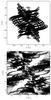 |
Fig. 1 uv-coverage of GMRT observations of MACS0025. Top: full uv-range. Bottom: zoom on the central portion of the uv-plane, illustrating the coverage on short baselines. Only one out of every ten data points are plotted. |
Throughout all observations, a minimum of 28 antennas were functional; any missing antennas were taken for painting or down due to problems with the hardware. Two major failures occurred during the observing runs; antenna fringe failures on 12th January resulted in a system reset and significant power issues occurred during the first hour of observing on 1st February. Compromised data were discarded for a total integration time on target of approximately 12 h. A summary of each night’s observations, including integration time, number of working antennas and any general comments are listed in Table 1.
On each night, the observations of the interleaved phase calibrator (0018-127; selected from the VLA calibrator manual1) and target (MACS0025) were bracketed at the beginning and end of the run by a 15-min scan on a primary calibrator source: either 3C 147, 3C 48 or 3C 468.1, depending on availability. The final uv-coverage of the GMRT observations of MACS0025 is shown in Fig. 1, where both the full uv-plane and a zoom on the short (<5kλ) baselines is presented.
2.1.2. Data reduction
The data were reduced using the Source Peeling and Atmospheric Modelling (SPAM) software (Intema et al. 2009) which employs NRAO Astronomical Image Processing Software (AIPS) tasks through the ParselTongue interface (Kettenis et al. 2006). SPAM employs the Scaife & Heald (2012; hereafter SH12) flux density scale, which provides models for a set of six calibrator sources designed to be used at low frequencies (particularly with LOFAR; van Haarlem et al. 2013). These sources all have flux densities that are stable over long periods, with well-understood spectral energy distributions (SED) and are compact compared to the resolution of LOFAR, to enable use of simple calibration models. In SH12, calibrators are selected from the 3C (Edge et al. 1959) and revised 3C (3CR; Bennett 1962) catalogues based on three criteria. Firstly, they must be at declination north of δ =20°. Secondly, they must have an integrated flux density greater than 20 Jy at 178 MHz and thirdly, they must have an angular diameter less than 20 arcsec.
The radio source 3C 468.1 is available as a bandpass calibrator for the GMRT, although it is less well documented than 3C 48, 3C 147 and 3C 286. 3C 468.1 is also not on the SH12 flux scale. However, flux density measurements between 38 MHz and 10.7 GHz are available from the literature, and in this work we use the measurements to extend the SH12 to include 3C 468.1 (see Appendix A).
Intema et al. (2009) describes data reduction with SPAM in detail; however here we will summarise the process. Following removal of edge channels, the data were averaged by a factor 4 in frequency (yielding 64 channels of width 502.8 kHz) and 2 in time, as a compromise between improving data processing speed and mitigating bandwidth-/time-smearing effects. Prior to calibration, the data were visually inspected for strong RFI and bad antennas/baselines. Calibration solutions were derived for the primary calibrators 3C 147, 3C 48 and 3C 468.1 and applied to the field, following standard techniques in SPAM. Properties of these calibrator sources are presented in Table 2.
The interleaved calibrator was not used during the reduction process – rather it was used to track data quality variation and atmospheric effects during the observing run itself. Instead, SPAM performs an initial phase calibration (and astrometry correction) using a sky model derived from the NRAO VLA Sky Survey (NVSS; Condon et al. 1998) before proceeding with three rounds of direction-independent phase-only self-calibration and imaging.
Properties of calibrator sources used in this work, with flux density measurements and spectral index values on the Scaife & Heald (2012) flux density scale.
Following the self-calibration, SPAM identifies strong sources within the primary beam FWHM that are suitable for direction-dependent calibration and ionospheric correction. Only sources with well-defined astrometry are selected, in this case yielding a catalogue of approximately 20 sources. Subsequently, SPAM performs direction-dependent calibration on a per-facet basis, using the solutions to fit a global ionospheric model, as described by Intema et al. (2009). Throughout the reduction process, multiple automated flagging routines are used between cycles of imaging and self-calibration in order to reduce residual RFI and clip outliers. Overall, 55 per cent of the data were flagged; whilst this is high, this level of flagging is not uncommon for GMRT data at this frequency.
2.1.3. Imaging
During the self-calibration and imaging cycles, images were made using an AIPS ROBUST of −1.0 as a trade-off between sensitivity and resolution. Note that an AIPS ROBUST = −5.0 indicates pure uniform weighting, for maximum resolution; ROBUST = + 5.0 indicates pure natural weighting, for maximum sensitivity. All imaging was performed with facet-based wide-field imaging as implemented in SPAM. Three different images were produced following calibration: a full-resolution image including the full uv-range, with an AIPS ROBUST−1.0; a high-resolution image made using baselines longer than 2kλ, made to filter out emission on ~Mpc scales; and a low-resolution image made after subtracting the clean-component model of the high-resolution image, with a uv-taper of 5kλ to improve sensitivity to diffuse emission.
In Fig. 2, we present the entire field-of-view of the GMRT observations of MACS0025, imaged with an AIPS ROBUST of −1.0. The MACS0025 field is rich, with many complex radio sources, including a number of radio galaxies (RG) hosting emission on a wide variety of scales. A number of these are highlighted in Fig. 2, and we discuss these sources further in Appendix B, where we present postage stamps of these sources (Fig. B.1) and mark any potential hosts identified in the literature. Given the locations of these sources and the redshifts of identified hosts, none of these are associated with MACS0025.
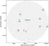 |
Fig. 2 Full field of view of the GMRT at 325 MHz and at a resolution of 10.1 × 8.3 arcsec. Image noise toward the field centre is 81 μJy beam-1. Colour scale saturates at 10 mJy beam-1 in order to emphasise emission from radio galaxies in the field. A number of the more extended radio galaxies are identified: these are further discussed in Appendix B. MACS0025 is also identified, as are the two brightest compact sources in the field, S1 and S2, which have integrated flux densities of 2.70 ± 0.27 and 0.94 ± 0.09 Jy, respectively, at 325 MHz. |
Additionally, there are two bright radio sources located reasonably far to the south of the field centre. These are identified as S1 and S2 in Fig. 2; in the literature they are known respectively as PKS 0023−13 and MRC 0023−12B. With integrated flux densities of 2.70 ± 0.27 and 0.94 ± 0.09 Jy for S1 and S2 respectively (measured using imfit in CASA 4.1), these sources caused severe artefacts in the field. While calibration with SPAM has significantly reduced these artefacts, our dynamic range is still limited. We measure an image noise of 81 μJy beam-1 toward the field centre, whereas the predicted thermal noise for this observation is approximately 20 μJy beam-1.
2.2. Chandra data
2.2.1. Observations
MACS0025 has been observed a total of five times by Chandra with the Advanced CCD Imaging Spectrometer (ACIS; Garmire et al. 2003). All exposures were taken with the ACIS-I imaging configuration and therefore have uniform spectral properties. We have extracted and reprocessed all of this existing data for the subsequent analysis. Table 3 lists the relevant characteristics of the individual exposures.
Observation log of Chandra data for MACS0025.
2.2.2. Data reduction
The individual datasets were reprocessed using CIAO 4.6 and CALDB 4.6.1.1 to apply the latest gain and calibration corrections. Standard filtering was applied to the event files to remove bad grades and pixels. Each of the individual ObsIDs were also examined for the presence of strong background flares. None of the exposures showed evidence for appreciable flare events, however, so no additional filtering was required. These reprocessed event files were used in all subsequent imaging and spectral analyses. The final, combined exposure time after all filtering was 156.6 ks.
2.2.3. Imaging
A surface brightness mosaic of the field around MACS0025 was constructed by re-projecting the individual event files to a common tangent point on the sky and then combining them. To correct for sensitivity variations across the field, instrument and exposure maps were made for each ObsID individually and combined after re-projection to flat-field the resulting mosaic.
For the instrument maps, the spectral weighting was determined by fitting a single temperature, MEKAL thermal model (Mewe et al. 1985; Liedahl et al. 1995) plus foreground Galactic absorption to the total integrated spectrum from the central 90 arcsec region around MACS0025. The Galactic absorption was modelled as neutral gas with solar abundances and a column density fixed at NH = 2.38×1020 cm-2 as determined by the LAB Survey of Galactic H I (Kalberla et al. 2005). This model gives a reasonable fit to the data with a reduced χ2 = 1.04 and best-fit temperature and metallicity of kT = 8.5 keV and Z = 0.23, respectively.
Individual background event files were created for each dataset from the standard ACIS blank-sky event files following the procedure described in Vikhlinin et al. (2005) and combined after re-projection to form a background mosaic. The resulting background-subtracted, exposure-corrected mosaic for the energy range 0.5−7.0 keV is shown in Fig. 3.
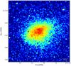 |
Fig. 3 Exposure-corrected, background-subtracted 0.5−7.0 keV surface brightness mosaic for the central region around MACS0025 based on 156 ks of existing Chandra archival data. The field measures 5 × 5 arcmin2 and has been smoothed with a σ ~ 3″ Gaussian. |
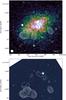 |
Fig. 4 Composite images of MACS0025. Top panel: colour image is X-ray surface brightness as per Fig. 3. Bottom panel: colour image is HST image of the cluster centre (proposal 10703, P.I. H. Ebeling). Cyan boxes identify optical hosts for the compact radio sources. In both panels, contours are 325 MHz GMRT data, imaged with an AIPS ROBUST −1.0, at levels [1, 2, 4, 8, 16, 32, 64] ×5σFR where σFR = 81 μJy beam-1. The −5σ contour is presented in gray. The synthesised beam is 10.1 × 8.3 arcsec at PA 51.1°, indicated by the unfilled ellipse in the lower-left corner. |
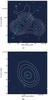 |
Fig. 5 Postage stamps of radio/optical associations for compact radio sources in MACS0025. Panel a) presents the triplet of compact radio sources in the SE sub-cluster of MACS0025, panel b) presents the single compact radio source in the NW sub-cluster. Contours are full-resolution GMRT data as per Fig. 4. The colour-scale is HST data as per Fig. 4. All selected optical hosts (cyan boxes) are cluster member galaxies, identified as absorption-line ellipticals by Ma et al. (2010). |
2.2.4. Spectral analysis
We have performed spatially-resolved spectral analyses of the X-ray emission in MACS0025 considering both 1D and 2D adaptive binning. For the 2D analysis, the contour binning algorithm of Sanders (2006) was used, while for the 1D analysis a series of radially symmetric annuli were defined, centred on the peak of the X-ray flux density (00h25m29.380s-12°22′37.06′′). We note that due to the combination of the adaptive binning process and the signal-to-noise requirement on the extracted spectra, the definition of the resulting extraction regions are relatively insensitive to the exact choice of X-ray centroid. In both cases, all spectral extraction regions were defined adaptively so as to contain a specified signal-to-noise ratio after background subtraction. Within each region, source and background spectra, effective area, and response matrix files were created for each OBSID individually and then combined into a single, summed set of files for analysis using the CIAO tool combine_spectra. All subsequent spectral analysis was done using the Sherpa (Freeman et al. 2001) fitting package in CIAO.
3. Results
We present multi-wavelength images of MACS0025 in Fig. 4. Contours correspond to the full-resolution (AIPS ROBUST −1.0) radio data at 325 MHz from the GMRT. In the top panel, the colour image is the X-ray surface brightness from archival Chandra data as per Fig. 3 (details of which are shown in Table 3) displayed using the “cubehelix” colour scheme (Green 2011). The bottom panel presents the optical image of MACS0025 from HST data (proposal 10703, P.I. H. Ebeling) reduced using the default HST pipeline. The synthesised beam of the full-resolution GMRT image is 10.1 × 8.3 arcsec; the measured off-source noise is 81 μJy beam-1.
3.1. Radio-optical cross identification
From Fig. 4, it can be seen that we recover emission from multiple compact sources in the region of MACS0025, and that there is little indication of any diffuse emission at this resolution. The triplet of compact radio sources south-east of the cluster centre all appear to be associated with cluster-member galaxies, as identified by Bradač et al. (2008) and Ma et al. (2010). Figure 5 presents postage stamp images of the compact radio sources in MACS0025.
The host galaxies of two of the compact radio sources to the SE of MACS0025 are the two BCGs in this sub-cluster (as identified by Bradač et al. 2008). These BCGs are identified in Fig. 5a. Additionally, from Fig. 4 the central radio source of the triplet appears to be associated with a faint X-ray point source, which may suggest a powerful AGN. Their optical spectra indicate that the hosts of these compact radio sources are all absorption-line elliptical galaxies (Ma et al. 2010).
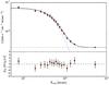 |
Fig. 6 Extracted surface brightness profile for MACS0025. In the upper panel, the solid line shows the best-fit model to the overall surface brightness. The background level is denoted by the horizontal, dashed line while the dotted curve indicates the underlying, background-subtracted model. The lower panel indicates the difference between data and model relative to the error at each radius. For both panels, the radius, Rmaj, corresponds to the radial distance along the semi-major axis of the assumed elliptical distribution. The model is discussed in the text. |
3.2. X-ray surface brightness profile
The X-ray surface brightness distribution in MACS0025 shows a clear elliptical structure with the major axis of the ellipse oriented along what is presumed to be the merger axis in the system (see Fig. 3). A radial surface brightness profile was computed by defining a set of elliptical annuli centered on the peak of the X-ray emission. As discussed above, these annuli have been defined adaptively to include a minimum number of counts after background subtraction, thereby assuring a uniform signal-to-noise ratio (SNR) in each bin. A fixed axial ratio of b/a = 2 was assumed, where b and a are taken to be the major and minor axes of the elliptical distribution, respectively. The position angle (PA) of the X-ray emission was taken to be 120° as measured counter-clockwise from north.
The resulting elliptical surface brightness profile is shown in Fig. 6. An isothermal β profile (Cavaliere & Fusco-Femiano 1976; Sarazin & Bahcall 1977) of the form: 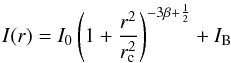 (1)provides a reasonable representation of the azimuthally averaged surface brightness profile where I0, rc and β are the peak central surface brightness, core radius and exponential fall-off at large radii, respectively. IB is a constant representing the contribution of the background. Given this model, we find best-fit values of I0 = 6.42 ± 0.14×10⁻⁸ cnts s-1 cm-2, rc = 72″ ± 3″ and β = 0.94 ± 0.04 for these parameters. The corresponding best-fit value for the background surface brightness is IB = 2.85 ± 0.01×10⁻⁹ cnts s-1 cm-2.
3.3. Mass profiles
As we discuss in Sect. 4.1.2, de Gasperin et al. (2014) find evidence for a correlation between the observed 1.4 GHz radio power for large-scale radio relics observed in clusters and the mass of the host cluster as inferred from SZ measurements with Planck (Planck Collaboration XXIX 2014). For an assumed spectral index, we can, in principle, use the GMRT observations presented here to assess whether the observed power of the radio relics in the MACS0025 cluster is consistent with this correlation. Unlike the sample presented in de Gasperin et al. (2014), however, the MACS0025 cluster was not detected by Planck, so no SZ-derived mass estimates are available. Here, we have instead utilized the observed X-ray properties to derive a mass for the cluster, under the assumption of hydrostatic equilibrium.
 |
Fig. 7 Integrated mass profiles, M( <r), for MACS J0025.4−1222 assuming hydrostatic equilibrium and a prolate, ellipsoidal geometry. The upper curve represents the total gravitating mass within radius, r, and the lower curve gives the total gas mass. The vertical dotted line indicates the R500 radius as discussed in the text. |
Given radial profiles for the gas properties in MACS0025, we can derive both the gas mass and total gravitating mass in the MACS0025 system. Assuming hydrostatic equilibrium and spherical symmetry, the total cluster mass, M, contained with a radius r is given by  (2)where T(r) and ne(r) are the gas temperature and electron number density at radius r, respectively (Fabricant et al. 1980). Similarly, the gas mass can be calculated directly using
  (3)where dV is the volume of the shell containing gas at density ne(r), and μmp is the mean mass per particle 1.0 × 10⁻²⁴ g.
In order to determine kT and ne as a function of position in the cluster, we have extracted spectra for a series of elliptical annuli centered on the peak of the X-ray emission for the ellipsoidal geometry described in Sect. 3.2. We have used a SNR criteria of 40 which results in ~1600 net counts per bin after background subtraction in each region. Within each extraction region, a single temperature, MEKAL thermal model (Mewe et al. 1985; Liedahl et al. 1995) was fitted to the combined spectrum from that region. The absorption was set to the nominal Galactic value of NH = 2.38×1020 cm-2 and the abundance was fixed to a value of Z = 0.23 based on the fit to the mean spectrum as discussed in Sect. 2.2.3.
The gas temperature kT at each radius is determined from the spectral fit directly. The electron density, ne, can be calculated directly from the normalisation of the fitted MEKAL model using  (4)where DA is the angular diameter distance at the cluster redshift z. For the assumed ellipsoidal geometry, the projected volume associated with each annulus can be estimated as (2/3) SL where S is the area of a given elliptical annulus with inner and outer semi-major axes of r1 and r2, respectively. The longest line-of-sight distance through the volume is denoted by L and, assuming a prolate ellipsoidal geometry with major to minor axis ratio of 2, can be expressed as
  (Henry et al. 2004; Mahdavi et al. 2005). This approximate method of deprojection assumes that the emission along the line-of-sight is dominated by material in the volume and that the contribution from material in front and behind the volume is negligible.
With these assumptions, the resulting total gas and gravitating mass as a function of radius along the cluster semi-major is shown in Fig. 7. Based on these profiles, we estimate a total gravitating mass M500 = 8.44 ± 3.16×10¹⁴M⊙, where R500 = 1.15 Mpc. This value agrees with the total mass estimate (lensing mass plus gas mass) Mtot = 5.65 ± 2.2×10¹⁴M⊙ from Bradač et al. (2008). We note that Bradač et al. (2008) measure the lensing masses within radii of 300 kpc of the sub-cluster BCGs, while the gas mass was measured within 500 kpc of the ICM X-ray peak.
3.4. Low-resolution radio imaging
To emphasise any diffuse emission associated with the cluster merger in MACS0025, we have subtracted the clean-component model of the compact radio sources associated with the cluster, made using the high-resolution image (not presented in this paper). Subsequently, the data were re-imaged, applying a uv-taper of 5 kλ to improve our sensitivity to large-scale radio emission. The cluster-member radio galaxies remain unresolved in both the full- and high-resolution images; consequently, flux density measurements are consistent between the full- and high-resolution images. As such, we are confident that any remaining flux density associated with these cluster member RG should be negligible.
The low-resolution, source-subtracted image is presented in Fig. 8, where the synthesised beam size is 28.2 × 23.7 arcsec and the image rms is 270 μJy beam-1. As can be seen in Fig. 8, we recover significant radio emission associated with the ICM on large angular scales. This represents the first detection of significant diffuse radio emission from this cluster.
Two sources of diffuse emission are present in Fig. 8, to the north-west (NW) and south-east (SE) of the cluster centre. The NW (SE) source has largest angular size of approximately 100 (90) arcsec; at the redshift of MACS0025, this corresponds to a largest linear size (LLS) of 640 (577) kpc. This is consistent with the typical size of many radio relics (e.g. Bonafede et al. 2012; de Gasperin et al. 2014) and haloes (e.g. Venturi et al. 2007, 2008; Kale et al. 2013, 2015).
These sources both exhibit an approximately arc-like morphology, are located toward the cluster periphery, and appear perpendicular to the proposed merger axis. As such, we identify this as a candidate double-relic system, and refer henceforth to these sources as the NW and SE relic. We use the fitting routine fitflux (Green 2007) to measure the flux density of the diffuse radio sources in Fig. 8. We recover an integrated flux density of 6.54 ± 0.72(8.88 ± 1.01) mJy for the NW (SE) relic. The uncertainty here comes from the sum of five per cent of the integrated flux density plus the standard deviation of seven fits, plus the off-source image noise, added in quadrature.
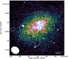 |
Fig. 8 Composite image of MACS0025. Colour plot is X-ray surface brightness as per Fig. 3. Contours are source-subtracted low-resolution GMRT data at 325 MHz, at levels [5, 7, 9, 11] ×σLR, where σLR = 270 μJy beam-1. The synthesised beam in the low-resolution image is 28.2 × 23.7 arcsec at PA 61.2°, indicated by the unfilled ellipse in the lower-left corner. |
4. Analysis
Given that this is the first detection of large-scale, diffuse radio emission from MACS0025, we cannot compare directly with previous work. As of January 2016, approximately 47 clusters are known to host radio relics, of which approximately 16 are known to host a pair of radio relics. In this section, we will examine how this new candidate double-relic system fits in with the known population. We include relics from both larger samples and surveys (e.g. Feretti et al. 2012; de Gasperin et al. 2014; Kale et al. 2015) as well as individual cluster studies (e.g. van Weeren et al. 2012; de Gasperin et al. 2015; Shimwell et al. 2015; Cantwell et al. 2016).
4.1. Proposed scenario: two radio relics
From both observations of clusters, as well as simulations, it is well established that major merger events with an approximately even mass ratio should generate pairs of outward-propagating shocks, which should consequently generate a pair of radio relics (e.g. van Weeren et al. 2011, although the merger they consider has a mass ratio of approximately 2:1). Previous observations of MACS0025 have suggested that the masses of the merging clusters are approximately equal: M ≃ 2.5×10¹⁴M⊙ (Bradač et al. 2008).
The morphology of the radio emission in Fig. 8 appears to be consistent with this interpretation, with both diffuse sources exhibiting approximately arc-like morphology. Additionally, both relics are detected at the periphery of the X-ray emission from the ICM, also consistent with both previous detections of relics and the suggestion that the merger event is occurring close to the plane of the sky (Bradač et al. 2008; Ma et al. 2010).
These relics have not been detected at other frequencies, so we cannot directly measure a spectral index. In the NVSS, emission is detected associated with the triplet of compact radio sources, but no emission is recovered at the 3σ level from the location of the NW relic. Likewise, we found no positive flux below the 3σ level in the NVSS image using fitflux; however, we can derive an upper limit from the surface brightness.
At 325 MHz, the emission from the NW relic peaks at 2.98 mJy beam-1, which corresponds to a surface brightness of approximately 15.7 μJy arcsec-2 given the beam size. Taking the 3σ limit from the NVSS (1.35 mJy beam-1, or ~ 2.4 μJy arcsec-2) implies an upper limit of α< −1.3 for the spectral index of the NW relic. This is consistent with the known population; for example, the “September 2011 relic collection” of Feretti et al. (2012) has a mean spectral index ⟨ α ⟩ = −1.3.
We use this spectral index to scale the flux density of our relics to 1.4 GHz and derive the radio power. Given the redshift of MACS0025 (z = 0.5857; Bradač et al. 2008) we find P1.4 GHz = 1.29 ± 0.14×1024 W Hz-1 for the NW relic and P1.4 GHz = 1.76 ± 0.20×1024 W Hz-1 for the SE relic, with our cosmology.
4.1.1. Power scaling: radio power vs. X-ray luminosity
In their review, Feretti et al. (2012) categorise cluster radio relics as “elongated” and “roundish”, with the former bearing the morphological hallmarks typical of the well-known giant radio relics, and the latter exhibiting a more rounded, regular morphology. Like elongated relics, roundish relics also exhibit steep spectra, an apparent lack of an optical counterpart, as well as a high polarisation fraction. Feretti et al. (2012) include radio phoenixes under the umbrella of roundish relics. Some examples of roundish relics are those in A584b (Feretti et al. 2006), AS753 (Subrahmanyan et al. 2003) and A1664 (Govoni et al. 2001). It is worth noting that no roundish relics have been detected beyond z ≃ 0.2, whereas MACS0025 is at redshift z = 0.5857 (Bradač et al. 2008). We do not include roundish relics in our analysis, as they may include a variety of different classes of source.
The X-ray luminosity of MACS0025 is Lx = 8.8 ± 0.2×1044 erg s-1 (Ebeling et al. 2007). In Fig. 9 we present the Lx/P1.4 GHz plane for galaxy clusters hosting radio relics in the literature. Clusters hosting single radio relics are marked in blue while those hosting a pair are marked in black. From Fig. 9, the relics hosted by MACS0025 are consistent with the known population.
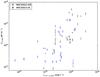 |
Fig. 9 Power scaling relation in the Lx/P1.4 GHz plane for galaxy cluster radio relics. Open circles indicate clusters hosting a pair of radio relics from the literature. Blue squares denote clusters hosting a single radio relic. Filled black (red) circles indicate the radio power and X-ray luminosity for the SE (NW) diffuse radio sources hosted by MACS0025. |
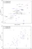 |
Fig. 10 Dependence of cluster relic radio power on a) cluster mass and b) redshift. Open circles indicate clusters hosting a pair of radio relics from the literature. Blue squares denote clusters hosting a single radio relic. Filled black (red) circles indicate the position of the SE (NW) diffuse radio sources hosted by MACS0025. The dashed red line in panel a) denotes the M500/P1.4 GHz relation from de Gasperin et al. (2014). Mass estimates are via the SZ-effect from the Planck cluster catalogue (Planck Collaboration XXIX 2014), or via a scaling relation based on the X-ray luminosity (Lx [0.1−2.4 keV]; de Gasperin et al. 2014) for all clusters except MACS0025, where the mass is derived in Sect. 3.3. |
4.1.2. Power scaling: radio power vs. cluster mass
de Gasperin et al. (2014) investigate the possibility of a relation between cluster mass (M500) derived via the Sunyaev-Zel’dovich effect from the Planck cluster catalogue (Planck Collaboration XXIX 2014) and radio power at 1.4 GHz, finding find a strong correlation. This relationship takes the form  for clusters hosting double-relics, and still holds (albeit with greater scatter) when clusters hosting a single relic are included.
In Fig. 10a we reproduce the data from de Gasperin et al. (2014) with the addition of a MACS0025 as well as some other clusters hosting relics that have been detected following de Gasperin et al. (2014). MACS0025 was not detected by Planck; instead we use the total gravitating mass derived from the X-ray data, M500 = 8.44 ± 3.16×10¹⁴M⊙.
We note that Czakon et al. (2015) find a mass estimate  ×1014M⊙ for MACS0025 from the Bolocam X-ray SZ (BOXSZ; Sayers et al. 2013) sample. However, this is measured over a smaller aperture than the mass measurements used by de Gasperin et al. (2014). From Fig. 10, the relics hosted by MACS0025 are consistent with the scatter in the M500/P1.4 GHz plane for known relics, although they lie far from the relation derived by de Gasperin et al. (2014).
4.1.3. Power scaling: radio power vs. redshift
In Fig. 10b we present the radio power at 1.4 GHz as a function of redshift for the known population of radio relics. The relics in MACS0025 appear to be consistent with the general trend between radio power and redshift. To date, only two other clusters beyond redshift z = 0.5 are known to host radio relics: MACS J1149.5+2223 at z = 0.544 (Bonafede et al. 2012) and ACT-CLJ0102−4915 at z = 0.855 (“El Gordo”; Lindner et al. 2014). For high-redshift clusters, MACS0025 appears to be slightly low in the P1.4 GHz/z plane, although this is likely due to selection effects and/or small number statistics.
In general, the apparent trend exhibited in the P1.4 GHz/z plane is severely impacted by selection effects – the surface brightness sensitivity of historic cluster studies has not been sufficient to detect faint relics at high redshift. The fact that the relics in MACS0025 lie slightly below the apparent correlation may suggest we are probing deeper than the majority of previous high-redshift cluster studies.
Overall, from Figs. 9 and 10 it is appears that the relics hosted by MACS0025 are consistent with established trends in power-scaling relations for the known population of relics. Note that the relic in MACS J2243.3−0935 (Cantwell et al. 2016) appears slightly low in all power-scaling planes; this may be due to the suggested nature as an infall relic rather than a relic generated by a merger shock, or a result of improved data reduction techniques.
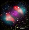 |
Fig. 11 False-colour image of MACS0025. Background image is a RGB optical image from HST. Cyan denotes the total mass distribution traced by lensing (dominated by the dark matter). Purple denotes the baryonic mass distribution (dominated by the ICM plasma). Red denotes the diffuse radio emission at 325 MHz. This image is in the J2000 coordinate system, north is up and east is to the left. X-ray and radio data are from this work whereas optical and lensing data are from Bradač et al. (2008). The scale bar denotes the angular extent corresponding to a physical distance of 0.5 Mpc at the redshift of MACS0025. |
5. Discussion
5.1. Bulk components of the ICM
In Fig. 11, we present a RGB optical image of MACS0025 taken with HST (from Bradač et al. 2008) overlain with false-colour multi-wavelength data. Figure 11 shows the relative distributions of the total mass (as traced by gravitational lensing, which is dominated by dark matter, from Bradač et al. 2008) and the baryonic mass (as traced by the X-ray surface brightness, based on the new analysis presented in this work). The lensing mass is shown in cyan and the baryonic mass in purple. Also overlain in red is the radio emission recovered by the GMRT at 325 MHz.
MACS0025 was the second galaxy cluster where significant separation was detected between the total mass and baryonic mass distributions. MACS0025 joins the Bullet cluster as part of a growing population of clusters that both host diffuse radio emission and exhibit clear separation between baryonic matter and dark matter components. Shan et al. (2010) derive the offset between the lensing and X-ray centroids for a sample of 38 galaxy clusters; in their sample are a small number of other galaxy clusters with significant offset (≳ 150 kpc) that are also known to host both a radio relic and halo: A2163 (Feretti et al. 2001) and A2744 (Govoni et al. 2001; Orrù et al. 2007).
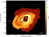 |
Fig. 12 X-ray temperature map of MACS0025, with low-resolution radio contours from the GMRT, as per Fig. 8. |
From Bradač et al. (2008) the offsets between the lensing peaks and the baryonic matter peak (defined as the X-ray centroid) are 0.5 and 0.82 arcmin; at the redshift of MACS0025, these correspond to a physical distance of 192 and 316 kpc, respectively, for the NW (SE) sub-cluster. These offsets are comparable to the offsets for the Bullet cluster (201 kpc), A2163 (141 kpc) and A2744 (238 kpc) from Shan et al. (2010). Note that this physical size is derived using our cosmology and the measured angular offsets from Shan et al. (2010).
5.2. Large-scale temperature structure
In order to search for signatures of the merger in the underlying temperature structure in MACS0025, we have performed a 2D spectral analysis. As mentioned previously, the spectral extraction regions were defined using the contour binning algorithm of Sanders (2006) based on the X-ray surface brightness image and such that each region had a fixed SNR. This technique trades off spectral accuracy against extraction region size and by extension the ability to resolve smaller-scale temperature structures. We have used a criteria of SNR~ 30 which results in approximately 900 net counts per bin after background subtraction in each region. This choice represents a compromise between obtaining reasonable accuracy in the fitted temperature values while simultaneously preserving modest angular resolution.
In each of the resulting extraction regions, the standard set of source spectrum, background spectrum, effective area and response matrix files were created for each OBSID contributing to that region. These individual files were then combined into a single set of summed files for each region with the CIAO tool combine_spectra and used for all subsequent fitting. At each point in the resulting map, we have fitted a single temperature, a MEKAL thermal model (Mewe et al. 1985; Liedahl et al. 1995) and foreground Galactic absorption to the combined spectrum from that region. The Galactic absorption was fixed to a value of NH = 2.38×1020 cm-2 as discussed previously in Sect. 2.2.3.
For the elemental abundance, we have derived temperature maps where the abundance was both fixed and allowed to vary spatially. The maps are qualitatively similar in both cases; however, the fitted abundances are not well-constrained in the spatially varying case and the errors on the derived temperature values are also higher. Given the higher temperature range (~6−10 keV) observed in MACS0025, the fits are relatively insensitive to the abundance. Consequently, to determine the best constraints on the temperature values, we have fixed the abundance to a value of Z = 0.23 based on the fit to the mean spectrum discussed above in Sect. 2.2.3. The final temperature map for MACS0025 is shown in Fig. 12.
The overall temperature structure shown in Fig. 12 appears, in general, consistent with the presence of a strong merger in MACS0025. We find regions of higher temperature approximately aligned with the merger axis. We have been cautious in interpreting the maps as the contour binning algorithm combined with the lower signal-to-noise of the data can tend to enhance apparent “shell-like” substructures in the temperature. With this caveat in mind, we note that the map shown in Fig. 12 does seem to exhibit preferentially hotter gas along the merger axis presumably due to shock heating associated with the merger. However, given the limitations of the data, and the fact that the typical error in Fig. 12 is of the order of 30 to 50 per cent, this correspondence must be seen as more suggestive than definitive.
5.3. Shocks in the ICM?
As can be seen in Fig. 12, we have a tentative detection of regions of enhanced temperature in the ICM of MACS0025. However, as discussed, the errors are sufficiently large that Mach number constraints from the X-ray data will not provide tight constraints on the viability of this being a merger shock.
Additionally, the temperature structure exhibited in Fig. 12 is reminiscent of a cold front, with the cooler (unshocked) region of gas downstream of the hotter (shocked) region. However, from earlier, there is no evidence of surface brightness discontinuity that is typically associated with cold fronts (see Markevitch & Vikhlinin 2007 for a thorough review of cold fronts in galaxy clusters).
We can estimate the Mach number based on the radio spectral index, following the formalism of Blandford & Eichler (1987). For simple shocks,  (5)where αinj is the power-law spectral index of cosmic ray electrons (CRe) at the shock front. Earlier, we estimated the upper limit spectral index to be α< −1.3; hence, Eq. (5) suggests a Mach number ℳ < 1.87. This is typical of the Mach numbers both predicted from simulations of cluster merger shocks and from observations at radio wavelengths, which suggest Mach numbers 1 ≤ ℳ ≤ 3 (e.g. Feretti et al. 2012; Brunetti & Jones 2014).
5.4. Should MACS0025 host a radio halo?
Whilst radio haloes and relics are strongly associated with merging clusters, the exact conditions necessary to generate these objects are far from clear. Cluster mergers deposit vast quantities of energy into the ICM and cause significant turbulence, yet not all merging clusters host a RH. Likewise, the link between merger shocks and relics is generally supported by observational evidence, but many merging clusters with prominent ICM shocks do not host relics.
Brunetti & Jones (2014) estimate the timescale required to generate a RH following the turbulent acceleration framework, deriving τacc ~ 100 Myr. Likewise, Brunetti & Jones (2014) estimate the lifetime of radio-emitting electrons for the Coma cluster using viable magnetic field estimates, deriving τCRe ~ few×100 Myr. For comparison, Brunetti et al. (2009) estimate the lifetime of RH based on a statistical sample of approximately 19 galaxy clusters, deriving τRH ~ 1.3 Gyr. Based on the optical properties of the cluster, Ma et al. (2010) conclude that core passage in MACS0025 occurred between 0.5 and 1 Gyr ago, suggesting that sufficient time should have elapsed to generate a RH.
From examination of double-relic systems in the literature, it appears that time since core passage (τCP) and mass ratio cannot be used alone to suggest whether or not a cluster should host a RH. For example, the system CIZA J2242.8+5301 (hereafter CIZAJ2242) hosts a pair of relics but no RH (e.g. van Weeren et al. 2010). Simulations suggest that this system involves a pair of merging clusters with a mass ratio approximately 2:1, with core passage occurring around 1 Gyr ago (van Weeren et al. 2011).
In contrast, El Gordo hosts a pair of relics and a halo (Lindner et al. 2014; Botteon et al. 2016b). Weak lensing observations of El Gordo suggest that the sub-clusters also have a mass ratio of approximately 2:1 (Jee et al. 2014). A dynamical analysis of what is known about El Gordo is presented by Ng et al. (2015), who indicate two potential scenarios for the merger in El Gordo: either the system is observed shortly after first core passage (τCP ~ 0.46 Gyr) or the clusters are again on approach, having turned around (τCP ~ 0.91 Gyr). Ng et al. (2015) suggest that the latter scenario is favoured if the time-averaged sub-cluster velocities exceed the shock velocity of the corresponding relic.
Both clusters also appear to have similar total masses: de Gasperin et al. (2014) find total masses Mtot = 7.97 ± 0.35×10¹⁴ (8.80 ± 0.66 × 10¹⁴) M⊙ for CIZAJ2242 (El Gordo). It should be noted that these mass measurements were derived through different means; via the SZ effect for El Gordo (Planck Collaboration XXIX 2014) and via the scaling relation between X-ray luminosity and total mass (Pratt et al. 2009) for CIZAJ2242. The velocity dispersions of the sub-clusters involved in the merger events also appear to be consistent: from Jee et al. (2014) the spectroscopically-measured velocity dispersions of the NW (SE) sub-cluster is σv = 1290 ± 134 (1089 ± 200) km s-1 for El Gordo, compared to  km s-1 (Dawson et al. 2015).
There is no evidence of a RH in MACS0025 at the 2σ level or higher, although an upper limit to the radio power can be derived. The sensitivity of the GMRT image at 325 MHz (Fig. 8) is 270 μJy beam-1. Given the restoring beam FWHM θ = 28.2×23.7 arcsec, the corresponding 2σ surface brightness limit SBlim = 1.03 μJy arcsec-2. Assuming a spherical geometry, a 1 Mpc RH would appear to be approximately 155 arcsec in diameter at the redshift of MACS0025, given the adopted cosmology. With a typical RH spectral index α = −1.3, this suggests a limiting radio power P1.4 GHz, lim ≃ 4×1024 W Hz-1. This does not place a tight constraint on the power of any potential RH in MACS0025.
The apparent lack of a RH in MACS0025 is not unexpected. For example, the statistical study of RH occurrence rates in clusters performed by Cuciti et al. (2015) suggests that only approximately 20 to 30 per cent of clusters with similar mass to MACS0025 host RH. Furthermore, previous surveys (e.g. Kale et al. 2015) indicate that there are many clusters in the luminosity range of MACS0025 which do not host a radio halo.
6. Conclusions
In this paper, we have presented the first deep radio observations of the high-redshift merging cluster MACS J0025.4−1222, performed using the GMRT at 325 MHz. The large FOV allows us to detect a population of radio galaxies that exhibit a wide range of morphologies. We also present a new analysis of all available Chandra X-ray data on this cluster.
Following subtraction of the compact radio source population, we recover two sources of diffuse emission on scales of several hundred kpc. Based on their location toward the cluster outskirts and their approximately arc-like morphology, we believe that this constitutes a new double-relic system, discovered for the first time in this cluster. We have shown that these relics are consistent with established power-scaling trends for the known relic population.
We derive an upper-limit spectral index α< −1.3 for the NW relic; this is consistent with the spectral index of known relics. This implies a Mach number that is also consistent with what is expected from weak shocks. The X-ray data exhibit an asymmetric surface brightness profile, extended along the merger axis; we also derive a 2D temperature map of MACS J0025.4−1222, which suggests the presence of regions of enhanced temperature along the merger axis.
We tentatively identify a region co-located with the NW relic that appears to exhibit a sharp temperature discontinuity. However, its structure is perhaps more reminiscent of a cold front than a merger shock, as the cooler region of gas lies downstream of the hotter region. The uncertainties on the X-ray temperature are too significant to provide tight constraints on the Mach number.
Available at http://aquarius.elte.hu/glade/
Acknowledgments
We thank our anonymous referee for their careful review, which has improved the quality of our manuscript. We also thank the operators and engineers of the GMRT who made these observations possible. The GMRT is operated by the National Centre for Radio Astrophysics (NCRA) of the Tata Institute of Fundamental Research (TIFR), India. CJR wishes to thank H. Intema for many helpful conversations during the data reduction process. C.J.R. gratefully acknowledges funding support from the United Kingdom Science and Technology Facilities Council (STFC). A.M.S. gratefully acknowledges support from the European Research Council under grant ERC-2012-StG-307215 LODESTONE. This work has made use of the NASA/IPAC Extragalactic Database (NED) and the NASA Astrophysics Data System (ADS). Many figures in this work have employed the “cubehelix” colour scheme (Green 2011).
References
- Akamatsu, H., de Plaa, J., Kaastra, J., et al. 2012a, PASJ, 64, 49 [NASA ADS] [Google Scholar]
- Akamatsu, H., Takizawa, M., Nakazawa, K., et al. 2012b, PASJ, 64, 67 [NASA ADS] [Google Scholar]
- Alam, S., Albareti, F. D., Allen de Prieto, C., et al. 2015, ApJS, 219, 12 [NASA ADS] [CrossRef] [Google Scholar]
- Baars, J. W. M., Genzel, R., Pauliny-Toth, I. I. K., & Witzel, A. 1977, A&A, 61, 99 [NASA ADS] [Google Scholar]
- Bennett, A. S. 1962, MmRAS, 68, 163 [Google Scholar]
- Blandford, R., & Eichler, D. 1987, Phys. Rep., 154, 1 [Google Scholar]
- Blasi, P., & Colafrancesco, S. 1999, Astropart. Phys., 12, 169 [NASA ADS] [CrossRef] [Google Scholar]
- Bonafede, A., Feretti, L., Giovannini, G., et al. 2009, A&A, 503, 707 [NASA ADS] [CrossRef] [EDP Sciences] [Google Scholar]
- Bonafede, A., Brüggen, M., van Weeren, R., et al. 2012, MNRAS, 426, 40 [NASA ADS] [CrossRef] [Google Scholar]
- Botteon, A., Gastaldello, F., Brunetti, G., & Dallacasa, D. 2016a, MNRAS, 460, L84 [NASA ADS] [CrossRef] [Google Scholar]
- Botteon, A., Gastaldello, F., Brunetti, G., & Kale, R. 2016b, MNRAS, 463, 1534 [NASA ADS] [CrossRef] [Google Scholar]
- Bradač, M., Clowe, D., Gonzalez, A. H., et al. 2006, ApJ, 652, 937 [NASA ADS] [CrossRef] [Google Scholar]
- Bradač, M., Allen, S. W., Treu, T., et al. 2008, ApJ, 687, 959 [NASA ADS] [CrossRef] [Google Scholar]
- Brunetti, G., & Jones, T. W. 2014, Int. J. Mod. Phys. D, 23, 30007 [Google Scholar]
- Brunetti, G., Setti, G., Feretti, L., & Giovannini, G. 2001, MNRAS, 320, 365 [NASA ADS] [CrossRef] [Google Scholar]
- Brunetti, G., Cassano, R., Dolag, K., & Setti, G. 2009, A&A, 507, 661 [NASA ADS] [CrossRef] [EDP Sciences] [Google Scholar]
- Cantwell, T. M., Scaife, A. M. M., Oozeer, N., Wen, Z. L., & Han, J. L. 2016, MNRAS, 458, 1803 [NASA ADS] [CrossRef] [Google Scholar]
- Cavaliere, A., & Fusco-Femiano, R. 1976, A&A, 49, 137 [NASA ADS] [Google Scholar]
- Clowe, D., Bradač, M., Gonzalez, A. H., et al. 2006, ApJ, 648, L109 [NASA ADS] [CrossRef] [Google Scholar]
- Cohen, A. S., Lane, W. M., Cotton, W. D., et al. 2007, AJ, 134, 1245 [NASA ADS] [CrossRef] [Google Scholar]
- Condon, J. J., Cotton, W. D., Greisen, E. W., et al. 1998, AJ, 115, 1693 [NASA ADS] [CrossRef] [Google Scholar]
- Conway, R. G., Kellermann, K. I., & Long, R. J. 1963, MNRAS, 125, 261 [NASA ADS] [CrossRef] [Google Scholar]
- Cuciti, V., Cassano, R., Brunetti, G., et al. 2015, A&A, 580, A97 [NASA ADS] [CrossRef] [EDP Sciences] [Google Scholar]
- Cutri, R. M., Wright, E. L., Conrow, T., et al. 2014, VizieR Online Data Catalog: II/328 [Google Scholar]
- Czakon, N. G., Sayers, J., Mantz, A., et al. 2015, ApJ, 806, 18 [NASA ADS] [CrossRef] [Google Scholar]
- Dalya, G., Frei, Z., Galgoczi, G., Raffai, P., & de Souza, R. S. 2016, VizieR Online Data Catalog: VII/275 [Google Scholar]
- Dawson, W. A., Jee, M. J., Stroe, A., et al. 2015, ApJ, 805, 143 [NASA ADS] [CrossRef] [Google Scholar]
- De Breuck, C., Tang, Y., de Bruyn, A. G., Röttgering, H., & van Breugel, W. 2002, A&A, 394, 59 [NASA ADS] [CrossRef] [EDP Sciences] [Google Scholar]
- de Gasperin, F., van Weeren, R. J., Brüggen, M., et al. 2014, MNRAS, 444, 3130 [NASA ADS] [CrossRef] [Google Scholar]
- de Gasperin, F., Intema, H. T., van Weeren, R. J., et al. 2015, MNRAS, 453, 3483 [NASA ADS] [CrossRef] [Google Scholar]
- Dennison, B. 1980, ApJ, 239, L93 [NASA ADS] [CrossRef] [Google Scholar]
- Douglas, J. N., Bash, F. N., Bozyan, F. A., Torrence, G. W., & Wolfe, C. 1996, AJ, 111, 1945 [NASA ADS] [CrossRef] [Google Scholar]
- Ebeling, H., Edge, A. C., & Henry, J. P. 2001, ApJ, 553, 668 [Google Scholar]
- Ebeling, H., Barrett, E., Donovan, D., et al. 2007, ApJ, 661, L33 [NASA ADS] [CrossRef] [Google Scholar]
- Edge, D. O., Shakeshaft, J. R., McAdam, W. B., Baldwin, J. E., & Archer, S. 1959, MmRAS, 68, 37 [Google Scholar]
- Fabricant, D., Lecar, M., & Gorenstein, P. 1980, ApJ, 241, 552 [NASA ADS] [CrossRef] [Google Scholar]
- Fanaroff, B. L., & Riley, J. M. 1974, MNRAS, 167, 31 [NASA ADS] [CrossRef] [Google Scholar]
- Feretti, L., Fusco-Femiano, R., Giovannini, G., & Govoni, F. 2001, A&A, 373, 106 [NASA ADS] [CrossRef] [EDP Sciences] [Google Scholar]
- Feretti, L., Bacchi, M., Slee, O. B., et al. 2006, MNRAS, 368, 544 [NASA ADS] [CrossRef] [Google Scholar]
- Feretti, L., Giovannini, G., Govoni, F., & Murgia, M. 2012, A&ARv, 20, 54 [Google Scholar]
- Ferrari, C., Govoni, F., Schindler, S., Bykov, A. M., & Rephaeli, Y. 2008, Space Sci. Rev., 134, 93 [NASA ADS] [CrossRef] [Google Scholar]
- Finoguenov, A., Sarazin, C. L., Nakazawa, K., Wik, D. R., & Clarke, T. E. 2010, ApJ, 715, 1143 [NASA ADS] [CrossRef] [Google Scholar]
- Freeman, P., Doe, S., & Siemiginowska, A. 2001, in Astronomical Data Analysis, eds. J.-L. Starck, & F. D. Murtagh, Proc. SPIE, 4477, 76 [Google Scholar]
- Garmire, G. P., Bautz, M. W., Ford, P. G., Nousek, J. A., & Ricker, Jr., G. R. 2003, in X-Ray and Gamma-Ray Telescopes and Instruments for Astronomy, eds. J. E. Truemper, & H. D. Tananbaum, SPIE Conf. Ser., 4851, 28 [Google Scholar]
- Gopal-Krishna, & Wiita, P. J. 2000, A&A, 363, 507 [NASA ADS] [Google Scholar]
- Govoni, F., Feretti, L., Giovannini, G., et al. 2001, A&A, 376, 803 [NASA ADS] [CrossRef] [EDP Sciences] [Google Scholar]
- Govoni, F., Murgia, M., Feretti, L., et al. 2005, A&A, 430, L5 [NASA ADS] [CrossRef] [EDP Sciences] [Google Scholar]
- Gower, J. F. R., Scott, P. F., & Wills, D. 1967, MmRAS, 71, 49 [NASA ADS] [Google Scholar]
- Green, D. A. 2007, Bull. Astron. Soc. India, 35, 77 [Google Scholar]
- Green, D. A. 2011, Bull. Astron. Soc. India, 39, 289 [Google Scholar]
- Gregory, P. C., & Condon, J. J. 1991, ApJS, 75, 1011 [NASA ADS] [CrossRef] [Google Scholar]
- Hales, S. E. G., Waldram, E. M., Rees, N., & Warner, P. J. 1995, MNRAS, 274, 447 [NASA ADS] [CrossRef] [Google Scholar]
- Henry, J. P., Finoguenov, A., & Briel, U. G. 2004, ApJ, 615, 181 [NASA ADS] [CrossRef] [Google Scholar]
- Intema, H. T., van der Tol, S., Cotton, W. D., et al. 2009, A&A, 501, 1185 [NASA ADS] [CrossRef] [EDP Sciences] [Google Scholar]
- Jaffe, W. J. 1977, ApJ, 212, 1 [NASA ADS] [CrossRef] [Google Scholar]
- Jee, M. J., Hughes, J. P., Menanteau, F., et al. 2014, ApJ, 785, 20 [NASA ADS] [CrossRef] [Google Scholar]
- Kalberla, P. M. W., Burton, W. B., Hartmann, D., et al. 2005, A&A, 440, 775 [NASA ADS] [CrossRef] [EDP Sciences] [Google Scholar]
- Kale, R., Venturi, T., Giacintucci, S., et al. 2013, A&A, 557, A99 [NASA ADS] [CrossRef] [EDP Sciences] [Google Scholar]
- Kale, R., Venturi, T., Giacintucci, S., et al. 2015, A&A, 579, A92 [NASA ADS] [CrossRef] [EDP Sciences] [Google Scholar]
- Kassim, N. E., Lazio, T. J. W., Erickson, W. C., et al. 2007, ApJS, 172, 686 [NASA ADS] [CrossRef] [Google Scholar]
- Kellermann, K. I. 1964, ApJ, 140, 969 [NASA ADS] [CrossRef] [Google Scholar]
- Kellermann, K. I., & Pauliny-Toth, I. I. K. 1973, AJ, 78, 828 [NASA ADS] [CrossRef] [Google Scholar]
- Kellermann, K. I., Pauliny-Toth, I. I. K., & Williams, P. J. S. 1969, ApJ, 157, 1 [NASA ADS] [CrossRef] [Google Scholar]
- Kerton, C. R. 2006, MNRAS, 373, 1203 [NASA ADS] [CrossRef] [Google Scholar]
- Kettenis, M., van Langevelde, H. J., Reynolds, C., & Cotton, B. 2006, in Astronomical Data Analysis Software and Systems XV, eds. C. Gabriel, C. Arviset, D. Ponz, & S. Enrique, ASP Conf. Ser., 351, 497 [Google Scholar]
- Konar, C., Hardcastle, M. J., Jamrozy, M., Croston, J. H., & Nandi, S. 2012, MNRAS, 424, 1061 [NASA ADS] [CrossRef] [Google Scholar]
- Lane, W. M., Cotton, W. D., van Velzen, S., et al. 2014, MNRAS, 440, 327 [NASA ADS] [CrossRef] [Google Scholar]
- Leahy, J. P., Black, A. R. S., Dennett-Thorpe, J., et al. 1997, MNRAS, 291, 20 [NASA ADS] [Google Scholar]
- Liedahl, D. A., Osterheld, A. L., & Goldstein, W. H. 1995, ApJ, 438, L115 [NASA ADS] [CrossRef] [Google Scholar]
- Lindner, R. R., Baker, A. J., Hughes, J. P., et al. 2014, ApJ, 786, 49 [NASA ADS] [CrossRef] [Google Scholar]
- Ma, C.-J., Ebeling, H., Marshall, P., & Schrabback, T. 2010, MNRAS, 406, 121 [NASA ADS] [CrossRef] [Google Scholar]
- Macario, G., Markevitch, M., Giacintucci, S., et al. 2011, ApJ, 728, 82 [NASA ADS] [CrossRef] [Google Scholar]
- Mahdavi, A., Finoguenov, A., Böhringer, H., Geller, M. J., & Henry, J. P. 2005, ApJ, 622, 187 [Google Scholar]
- Markevitch, M., & Vikhlinin, A. 2007, Phys. Rep., 443, 1 [NASA ADS] [CrossRef] [EDP Sciences] [Google Scholar]
- Mewe, R., Gronenschild, E. H. B. M., & van den Oord, G. H. J. 1985, A&AS, 62, 197 [NASA ADS] [Google Scholar]
- Ng, K. Y., Dawson, W. A., Wittman, D., et al. 2015, MNRAS, 453, 1531 [NASA ADS] [CrossRef] [Google Scholar]
- Ogrean, G. A., Brüggen, M., van Weeren, R. J., et al. 2013, MNRAS, 433, 812 [NASA ADS] [CrossRef] [Google Scholar]
- Orrù, E., Murgia, M., Feretti, L., et al. 2007, A&A, 467, 943 [NASA ADS] [CrossRef] [EDP Sciences] [Google Scholar]
- Orrù, E., van Velzen, S., Pizzo, R. F., et al. 2015, A&A, 584, A112 [NASA ADS] [CrossRef] [EDP Sciences] [Google Scholar]
- Paul, S., Datta, A., & Intema, H. T. 2014, ArXiv e-prints [arXiv:1412.0285] [Google Scholar]
- Pauliny-Toth, I. I. K., Wade, C. M., & Heeschen, D. S. 1966, ApJS, 13, 65 [NASA ADS] [CrossRef] [Google Scholar]
- Petrosian, V. 2001, ApJ, 557, 560 [NASA ADS] [CrossRef] [Google Scholar]
- Pizzo, R. F., de Bruyn, A. G., Bernardi, G., & Brentjens, M. A. 2011, A&A, 525, A104 [NASA ADS] [CrossRef] [EDP Sciences] [Google Scholar]
- Planck Collaboration XXIX. 2014, A&A, 571, A29 [NASA ADS] [CrossRef] [EDP Sciences] [Google Scholar]
- Pratt, G. W., Croston, J. H., Arnaud, M., & Böhringer, H. 2009, A&A, 498, 361 [NASA ADS] [CrossRef] [EDP Sciences] [Google Scholar]
- Rengelink, R. B., Tang, Y., de Bruyn, A. G., et al. 1997, A&AS, 124, 259 [NASA ADS] [CrossRef] [EDP Sciences] [Google Scholar]
- Roger, R. S., Costain, C. H., & Bridle, A. H. 1973, AJ, 78, 1030 [NASA ADS] [CrossRef] [Google Scholar]
- Roy, J., Gupta, Y., Pen, U.-L., et al. 2010, Exp. Astron., 28, 25 [NASA ADS] [CrossRef] [Google Scholar]
- Saikia, D. J., & Jamrozy, M. 2009, Bull. Astron. Soc. India, 37, 63 [NASA ADS] [Google Scholar]
- Sanders, J. S. 2006, MNRAS, 371, 829 [NASA ADS] [CrossRef] [Google Scholar]
- Sarazin, C. L., & Bahcall, J. N. 1977, ApJS, 34, 451 [NASA ADS] [CrossRef] [Google Scholar]
- Sayers, J., Czakon, N. G., Mantz, A., et al. 2013, ApJ, 768, 177 [NASA ADS] [CrossRef] [Google Scholar]
- Scaife, A. M. M., & Heald, G. H. 2012, MNRAS, 423, L30 [NASA ADS] [CrossRef] [Google Scholar]
- Schilizzi, R. T., Tian, W. W., Conway, J. E., et al. 2001, A&A, 368, 398 [NASA ADS] [CrossRef] [EDP Sciences] [Google Scholar]
- Schoenmakers, A. P., de Bruyn, A. G., Röttgering, H. J. A., van der Laan, H., & Kaiser, C. R. 2000, MNRAS, 315, 371 [NASA ADS] [CrossRef] [Google Scholar]
- Shan, H., Qin, B., Fort, B., et al. 2010, MNRAS, 406, 1134 [NASA ADS] [Google Scholar]
- Shimwell, T. W., Markevitch, M., Brown, S., et al. 2015, MNRAS, 449, 1486 [NASA ADS] [CrossRef] [Google Scholar]
- Subrahmanyan, R., Beasley, A. J., Goss, W. M., Golap, K., & Hunstead, R. W. 2003, AJ, 125, 1095 [NASA ADS] [CrossRef] [Google Scholar]
- van Haarlem, M. P., Wise, M. W., Gunst, A. W., et al. 2013, A&A, 556, A2 [NASA ADS] [CrossRef] [EDP Sciences] [Google Scholar]
- van Weeren, R. J., Röttgering, H. J. A., Brüggen, M., & Cohen, A. 2009, A&A, 505, 991 [NASA ADS] [CrossRef] [EDP Sciences] [Google Scholar]
- van Weeren, R. J., Röttgering, H. J. A., Brüggen, M., & Hoeft, M. 2010, Science, 330, 347 [NASA ADS] [CrossRef] [PubMed] [Google Scholar]
- van Weeren, R. J., Brüggen, M., Röttgering, H. J. A., & Hoeft, M. 2011, MNRAS, 418, 230 [Google Scholar]
- van Weeren, R. J., Röttgering, H. J. A., Intema, H. T., et al. 2012, A&A, 546, A124 [NASA ADS] [CrossRef] [EDP Sciences] [Google Scholar]
- Venturi, T., Giacintucci, S., Brunetti, G., et al. 2007, A&A, 463, 937 [NASA ADS] [CrossRef] [EDP Sciences] [Google Scholar]
- Venturi, T., Giacintucci, S., Dallacasa, D., et al. 2008, A&A, 484, 327 [NASA ADS] [CrossRef] [EDP Sciences] [Google Scholar]
- Vikhlinin, A., Markevitch, M., Murray, S. S., et al. 2005, ApJ, 628, 655 [NASA ADS] [CrossRef] [Google Scholar]
- White, R. L., & Becker, R. H. 1992, ApJS, 79, 331 [NASA ADS] [CrossRef] [Google Scholar]
- Wright, E. L. 2006, PASP, 118, 1711 [NASA ADS] [CrossRef] [Google Scholar]
- Wright, A. E., Griffith, M. R., Burke, B. F., & Ekers, R. D. 1994, ApJS, 91, 111 [NASA ADS] [CrossRef] [Google Scholar]
- Zhang, X., Zheng, Y., Chen, H., et al. 1997, A&AS, 121, 59 [NASA ADS] [CrossRef] [EDP Sciences] [Google Scholar]
Appendix A: An extension to the Scaife and Heald flux scale: 3C 468.1
The radio source 3C 468.1 is available as a primary calibrator for GMRT observations, although it is perhaps the least preferred primary calibrator. No other calibrator source was available for the initial flux calibrator scan for our observations, however. The SPAM calibration routine makes use of the SH12 flux density scale, which does not include 3C 468.1. To avoid potential issues associated with using different flux density scales, therefore, we follow the method adopted by SH12 to fit the available flux density measurements for 3C 468.1 and add it to the SH12 flux density scale.
Flux density measurements exist between 38 MHz and 10 GHz for 3C 468.1, with observations using a range of different flux density scales. Following SH12 we bring these measurements onto the flux scale of Roger et al. (1973; hereafter RCB). We present these measurements, along with the correction factor required to bring them onto the RCB scale, in Table A.1. All flux density measurements on the Baars scale were adjusted by interpolation of the values listed in Table 7 of Baars et al. (1977; hereafter B77).
For the Texas radio survey at 365 MHz, Douglas et al. (1996) find their flux density measurements to be consistent with a factor of 96 per cent of the B77 flux scale. Below 325 MHz, the conversion process is a little more complex. For measurements on the Kellermann et al. (1969; hereafter KPW) scale at 178 MHz, RCB give a conversion factor of 1.09. For the measurement from Gower et al. (1967) on the CKL scale (Conway et al. 1963) Table 7 of B77 was used to convert to the RCB scale and then onto the SH12 scale. For the measurements at 74 MHz using the VLA (Cohen et al. 2007 and Kassim et al. 2007) the B77 scale was used. Lane et al. (2014) find that a mean conversion factor of 1.1 is required to bring flux density measurements into line with the SH12 flux scale.
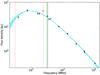 |
Fig. A.1 Integrated flux density of 3C 468.1 as a function of frequency. Dot-dashed line marks fourth-order polynomial fit to the data. Empty circle indicates measurement from the Miyun survey at 232 MHz which has been excluded from the fit. Shaded green region marks the frequency range covered by the GMRT observations in this work; shaded blue region marks 1σ uncertainty region on the model. Vertical dashed lines mark the frequency bounds of LOFAR. |
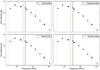 |
Fig. A.2 Polynomial spectral index models fitted to 3C 468.1, showing linear, second-, third- and fourth-order polynomial models from left to right. Empty circle indicates measurement from the Miyun survey at 232 MHz which has been excluded from the fit. Shaded green region marks the frequency range covered by the GMRT observations in this work; vertical dashed lines mark the frequency bounds of LOFAR. |
Polynomial spectral index model parameters for 3C 468.1.
We present the flux density measurements as a function of frequency in Fig. A.1. We exclude the 232 MHz flux density from the Miyun survey from the fitting partly due to a large discrepancy between the integrated flux density (43.98 Jy) and the peak flux density (38.77 Jy) and partly due to the large offset with respect to the other flux densities from the literature (see Fig. A.1). Following SH12, we attempt to fit a polynomial model in linear frequency space in order to retain Gaussian noise characteristics. As such, the functional form we attempt to fit is as follows: ![Mathematical equation: \appendix \setcounter{section}{1} \begin{equation} S \, [\rm{mJy}] = A_0 \prod_{i = 1}^{N} 10^{ A_i \, \log^i [\nu/150 \, \rm{MHz}]}. \end{equation}](/articles/aa/full_html/2017/01/aa29530-16/aa29530-16-eq210.png) (A.1)The best-fit parameters for linear, second-, third- and fourth-order polynomial functions are listed in Table A.2 (and presented in Fig. A.2) along with the associated uncertainties and the reduced chi-squared (
(A.1)The best-fit parameters for linear, second-, third- and fourth-order polynomial functions are listed in Table A.2 (and presented in Fig. A.2) along with the associated uncertainties and the reduced chi-squared ( ) which is used to evaluate the goodness of fit. From visual inspection it is clear that the linear and second-order models are a poor fit to the data; it also appears that a fourth-order polynomial describes the data marginally better at the low end of the frequency range.
In the case of 3C 468.1, selection of the best-fit model is heavily influenced by the confidence in the single data point at 38 MHz; this flux density measurement is from the revised 3C catalogue (3CR; Hales et al. 1995). Based on this, and the values, we select a fourth-order polynomial as the “best-fit” model for the spectral index behaviour of 3C 468.1. In Fig. A.1 we present the fourth-order fit to the data shown in Table A.1. The uncertainty in the model was derived using a Monte-Carlo simulation of the parameter space over 1000 iterations; in Fig. A.1 the 1σ uncertainty is indicated by the shaded cyan region.
Appendix B: Radio environment of MACS0025
In this Appendix we present postage stamp images of the extended radio sources identified in Fig. 2. For each RG, we again measured the flux density recovered by the GMRT using fitflux (Green 2007). These measurements are presented in Table B.1.
Measured parameters for extended radio sources in the MACS0025 field, as seen by the GMRT at 325 MHz.
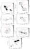 |
Fig. B.1 Postage stamp images of resolved sources in the GMRT field of view at 325 MHz. Contours start at 5σ and scale by a factor of two, where σ = 697/102/89/94/93/175/875 μJy beam-1 from top-left. Resolution is 10.1×8.3 arcsec, indicated by the hatched ellipse in the lower-left corner. Colour scales saturate at 100 mJy beam-1. Filled circles indicate the position of candidate host sources, where available. The scale bar denotes 200 kpc at the redshift of sources whose proposed hosts have measured z. |
Postage stamp images of these RG are presented in Fig. B.1, where contours start at 5σ and scale by a factor of two. The local noise for each postage stamp is noted in the caption of Fig. B.1. We have cross-referenced these sources with the literature to identify potential optical host galaxies and we will discuss them in this Appendix.
Approximately half of this field is covered by the 12th Data Release from the Sloan Digital Sky Survey (SDSS DR12; Alam et al. 2015) from which we identify optical host galaxies with photometric redshifts for four RG. None of these objects have spectroscopic redshifts. In Fig. B.1 filled circles indicate the location of any potential hosts.
Appendix B.1: RG1
This source appears to be a double-lobed radio source, with an approximate angular extent of 83 arcsec. We do not identify any candidate host galaxy for this radio source from the literature. The nearest source catalogued is AllWISE J002711.53−124819.1 (Cutri et al. 2014) although this appears to be co-located with the northern radio lobe, and is perhaps unlikely to host the observed radio emission.
Appendix B.2: RG2: a large-angular-size radio galaxy
The potential host for this source is identified as 2MASX J00265983−1218378 (RA 00h26m59.8s, Dec -12°18′38′′) at a redshift z = 0.153. From Fig. B.1, this host appears to be in a suitable position to host the radio emission. The angular distance between the hotspots of the radio lobes is of the order of 4.6 arcmin; with the cosmology we adopt in this work, this suggests a physical extent of the order of 705 kpc; slightly smaller than giant radio galaxies.
This source is well-resolved, with a marked difference in morphology between the northern and southern radio lobes. The northern lobe appears reasonably symmetric, whereas the southern lobe exhibits a highly asymmetric radio surface brightness. On the one hand, the asymmetry may indicate differences in the density of the local environment, which restricts the expansion of part of the southern lobe. On the other hand, this fainter region may be the remains of a radio lobe emitted during historic AGN activity, whereas the brighter region may be fresher plasma from a more recent phase of activity. The northern jet also exhibits a curious “kink”, which may be distorted due to the density profile of the local environment, or variation in the magnetic field orientation along the jet.
Appendix B.3: RG3: a hybrid-morphology radio source
RG3 is a complex case, exhibiting characteristics of both Fanaroff-Riley Class I (FR-I) and Class II (FR-II) radio galaxies (Fanaroff & Riley 1974). The eastern lobe appears relatively bright and amorphous, with no strong evidence of a jet (FR-II). In contrast, the radio emission to the west of the core appears to be more confined for a greater distance out from the central engine. Additionally, the radio emission appears to be connected to a bright central core by a jet. Finally, further to the west there is patchy emission that, if associated with this source, might suggest bending of the jet.
Sources with such mixed morphology are known as hybrid-morphology radio sources (HYMORS; Gopal-Krishna & Wiita 2000). A potential optical host is identified from the GLADE catalogue2 (Dalya et al. 2016). This source has a redshift z = 0.1617; at this redshift, the angular extent of this source (130 arcsec) corresponds to a physical extent of 347 kpc.
Appendix B.4: RG4
This source exhibits a curious morphology, reminiscent of the radio lobes of wide-angle-tail (WAT) RG seen in many galaxy clusters. However, no host is identified at a location consistent with this interpretation. Instead, we find a galaxy coincident with one of the “hotspots” in the NE region; SDSS J002315.60−123750.2 (z = 0.129), and no obvious host for the SW emission.
A number of other galaxies are identified by the SDSS in this region, although they are distributed across a broad enough redshift range (z = 0.108−0.414) that we cannot suggest that they form a group. If the radio emission is associated with SDSS J002315.60−123750.2, its angular extent (130 arcsec) corresponds to a physical distance of 287 kpc. The location of the host would then suggest that we are viewing this object in projection.
Appendix B.5: RG5
We identify a host galaxy for this object, SDSS J002314.06−121245.7 (z = 0.219). The angular extent of this source (78 arcsec) therefore corresponds to a physical extent of 266 kpc given our cosmology. At radio wavelengths, this source is also listed in the NVSS catalogue and 352 MHz WISH catalogue (De Breuck et al. 2002) under the identifiers NVSS 002313–121246 and WNB 0020.6–1229, respectively.
Appendix B.6: RG6: a candidate double-double radio galaxy
From the SDSS, we identify the host galaxy as SDSS J002239.44−114912.0 (z = 0.210). At this redshift, the angular extent of this source (170 arcsec) corresponds to a physical extent of 561 kpc.
When viewed in concert with the host location, the source morphology suggests that RG6 may be a double-double radio galaxy (DDRG). These sources exhibit themselves as pairs of double-lobed radio sources, where the lobes are aligned along the same axis and possess a common radio core (Schoenmakers et al. 2000). A number of other examples of DDRG exist in the literature (see for example Leahy et al. 1997; Schoenmakers et al. 2000; Schilizzi et al. 2001; Saikia & Jamrozy 2009; Konar et al. 2012; Orrù et al. 2015). DDRG are believed to arise as a result of recurrent AGN activity.
This source has also been identified in a number of radio surveys, including the 4.85 GHz Parkes-MIT-NRAO survey (PMN; Wright et al. 1994) under the identifier PMN J0022−1148, as well as the VLSS, WISH, and NVSS.
Appendix B.7: RG7
The morphology of this source is reminiscent of a classic double-lobed RG, with a pair of bright diametrically-opposed hotspots, and extended emission trails back toward the location of a central engine. This source has been catalogued by previous surveys between 74 MHz (VLSS) and 4.85 GHz (PMN). We identify a potential host galaxy for this source – SDSS J002150.58−123349.0. This source has a photometric redshift z = 0.382; at this redshift, the angular size of this source (83 arcsec) corresponds to a physical extent of 419 kpc.
All Tables
Properties of calibrator sources used in this work, with flux density measurements and spectral index values on the Scaife & Heald (2012) flux density scale.
Measured parameters for extended radio sources in the MACS0025 field, as seen by the GMRT at 325 MHz.
All Figures
|
Fig. 1 uv-coverage of GMRT observations of MACS0025. Top: full uv-range. Bottom: zoom on the central portion of the uv-plane, illustrating the coverage on short baselines. Only one out of every ten data points are plotted. |
| In the text | |
|
Fig. 2 Full field of view of the GMRT at 325 MHz and at a resolution of 10.1 × 8.3 arcsec. Image noise toward the field centre is 81 μJy beam-1. Colour scale saturates at 10 mJy beam-1 in order to emphasise emission from radio galaxies in the field. A number of the more extended radio galaxies are identified: these are further discussed in Appendix B. MACS0025 is also identified, as are the two brightest compact sources in the field, S1 and S2, which have integrated flux densities of 2.70 ± 0.27 and 0.94 ± 0.09 Jy, respectively, at 325 MHz. |
| In the text | |
|
Fig. 3 Exposure-corrected, background-subtracted 0.5−7.0 keV surface brightness mosaic for the central region around MACS0025 based on 156 ks of existing Chandra archival data. The field measures 5 × 5 arcmin2 and has been smoothed with a σ ~ 3″ Gaussian. |
| In the text | |
|
Fig. 4 Composite images of MACS0025. Top panel: colour image is X-ray surface brightness as per Fig. 3. Bottom panel: colour image is HST image of the cluster centre (proposal 10703, P.I. H. Ebeling). Cyan boxes identify optical hosts for the compact radio sources. In both panels, contours are 325 MHz GMRT data, imaged with an AIPS ROBUST −1.0, at levels [1, 2, 4, 8, 16, 32, 64] ×5σFR where σFR = 81 μJy beam-1. The −5σ contour is presented in gray. The synthesised beam is 10.1 × 8.3 arcsec at PA 51.1°, indicated by the unfilled ellipse in the lower-left corner. |
| In the text | |
|
Fig. 5 Postage stamps of radio/optical associations for compact radio sources in MACS0025. Panel a) presents the triplet of compact radio sources in the SE sub-cluster of MACS0025, panel b) presents the single compact radio source in the NW sub-cluster. Contours are full-resolution GMRT data as per Fig. 4. The colour-scale is HST data as per Fig. 4. All selected optical hosts (cyan boxes) are cluster member galaxies, identified as absorption-line ellipticals by Ma et al. (2010). |
| In the text | |
|
Fig. 6 Extracted surface brightness profile for MACS0025. In the upper panel, the solid line shows the best-fit model to the overall surface brightness. The background level is denoted by the horizontal, dashed line while the dotted curve indicates the underlying, background-subtracted model. The lower panel indicates the difference between data and model relative to the error at each radius. For both panels, the radius, Rmaj, corresponds to the radial distance along the semi-major axis of the assumed elliptical distribution. The model is discussed in the text. |
| In the text | |
|
Fig. 7 Integrated mass profiles, M( <r), for MACS J0025.4−1222 assuming hydrostatic equilibrium and a prolate, ellipsoidal geometry. The upper curve represents the total gravitating mass within radius, r, and the lower curve gives the total gas mass. The vertical dotted line indicates the R500 radius as discussed in the text. |
| In the text | |
|
Fig. 8 Composite image of MACS0025. Colour plot is X-ray surface brightness as per Fig. 3. Contours are source-subtracted low-resolution GMRT data at 325 MHz, at levels [5, 7, 9, 11] ×σLR, where σLR = 270 μJy beam-1. The synthesised beam in the low-resolution image is 28.2 × 23.7 arcsec at PA 61.2°, indicated by the unfilled ellipse in the lower-left corner. |
| In the text | |
|
Fig. 9 Power scaling relation in the Lx/P1.4 GHz plane for galaxy cluster radio relics. Open circles indicate clusters hosting a pair of radio relics from the literature. Blue squares denote clusters hosting a single radio relic. Filled black (red) circles indicate the radio power and X-ray luminosity for the SE (NW) diffuse radio sources hosted by MACS0025. |
| In the text | |
|
Fig. 10 Dependence of cluster relic radio power on a) cluster mass and b) redshift. Open circles indicate clusters hosting a pair of radio relics from the literature. Blue squares denote clusters hosting a single radio relic. Filled black (red) circles indicate the position of the SE (NW) diffuse radio sources hosted by MACS0025. The dashed red line in panel a) denotes the M500/P1.4 GHz relation from de Gasperin et al. (2014). Mass estimates are via the SZ-effect from the Planck cluster catalogue (Planck Collaboration XXIX 2014), or via a scaling relation based on the X-ray luminosity (Lx [0.1−2.4 keV]; de Gasperin et al. 2014) for all clusters except MACS0025, where the mass is derived in Sect. 3.3. |
| In the text | |
|
Fig. 11 False-colour image of MACS0025. Background image is a RGB optical image from HST. Cyan denotes the total mass distribution traced by lensing (dominated by the dark matter). Purple denotes the baryonic mass distribution (dominated by the ICM plasma). Red denotes the diffuse radio emission at 325 MHz. This image is in the J2000 coordinate system, north is up and east is to the left. X-ray and radio data are from this work whereas optical and lensing data are from Bradač et al. (2008). The scale bar denotes the angular extent corresponding to a physical distance of 0.5 Mpc at the redshift of MACS0025. |
| In the text | |
|
Fig. 12 X-ray temperature map of MACS0025, with low-resolution radio contours from the GMRT, as per Fig. 8. |
| In the text | |
|
Fig. A.1 Integrated flux density of 3C 468.1 as a function of frequency. Dot-dashed line marks fourth-order polynomial fit to the data. Empty circle indicates measurement from the Miyun survey at 232 MHz which has been excluded from the fit. Shaded green region marks the frequency range covered by the GMRT observations in this work; shaded blue region marks 1σ uncertainty region on the model. Vertical dashed lines mark the frequency bounds of LOFAR. |
| In the text | |
|
Fig. A.2 Polynomial spectral index models fitted to 3C 468.1, showing linear, second-, third- and fourth-order polynomial models from left to right. Empty circle indicates measurement from the Miyun survey at 232 MHz which has been excluded from the fit. Shaded green region marks the frequency range covered by the GMRT observations in this work; vertical dashed lines mark the frequency bounds of LOFAR. |
| In the text | |
|
Fig. B.1 Postage stamp images of resolved sources in the GMRT field of view at 325 MHz. Contours start at 5σ and scale by a factor of two, where σ = 697/102/89/94/93/175/875 μJy beam-1 from top-left. Resolution is 10.1×8.3 arcsec, indicated by the hatched ellipse in the lower-left corner. Colour scales saturate at 100 mJy beam-1. Filled circles indicate the position of candidate host sources, where available. The scale bar denotes 200 kpc at the redshift of sources whose proposed hosts have measured z. |
| In the text | |
Current usage metrics show cumulative count of Article Views (full-text article views including HTML views, PDF and ePub downloads, according to the available data) and Abstracts Views on Vision4Press platform.
Data correspond to usage on the plateform after 2015. The current usage metrics is available 48-96 hours after online publication and is updated daily on week days.
Initial download of the metrics may take a while.