| Issue |
A&A
Volume 596, December 2016
|
|
|---|---|---|
| Article Number | A43 | |
| Number of page(s) | 10 | |
| Section | The Sun | |
| DOI | https://doi.org/10.1051/0004-6361/201628649 | |
| Published online | 28 November 2016 | |
Non-magnetic photospheric bright points in 3D simulations of the solar atmosphere⋆
1 Istituto Ricerche Solari Locarno (IRSOL), via Patocchi 57 – Prato Pernice, 6605 Locarno-Monti, Switzerland
2 Geneva Observatory, University of Geneva, Ch. des Maillettes 51, 1290 Sauverny, Switzerland
e-mail: This email address is being protected from spambots. You need JavaScript enabled to view it.
3 Kiepenheuer-Institut für Sonnenphysik, Schöneckstrasse 6, 79104 Freiburg, Germany
4 Division of Astronomy and Space Physics, Department of Physics and Astronomy, Uppsala University, Box 516, 751 20 Uppsala, Sweden
Received: 6 April 2016
Accepted: 30 August 2016
Abstract
Context. Small-scale bright features in the photosphere of the Sun, such as faculae or G-band bright points, appear in connection with small-scale magnetic flux concentrations.
Aims. Here we report on a new class of photospheric bright points that are free of magnetic fields. So far, these are visible in numerical simulations only. We explore conditions required for their observational detection.
Methods. Numerical radiation (magneto-)hydrodynamic simulations of the near-surface layers of the Sun were carried out. The magnetic field-free simulations show tiny bright points, reminiscent of magnetic bright points, only smaller. A simple toy model for these non-magnetic bright points (nMBPs) was established that serves as a base for the development of an algorithm for their automatic detection. Basic physical properties of 357 detected nMBPs were extracted and statistically evaluated. We produced synthetic intensity maps that mimic observations with various solar telescopes to obtain hints on their detectability.
Results. The nMBPs of the simulations show a mean bolometric intensity contrast with respect to their intergranular surroundings of approximately 20%, a size of 60–80 km, and the isosurface of optical depth unity is at their location depressed by 80–100 km. They are caused by swirling downdrafts that provide, by means of the centripetal force, the necessary pressure gradient for the formation of a funnel of reduced mass density that reaches from the subsurface layers into the photosphere. Similar, frequently occurring funnels that do not reach into the photosphere, do not produce bright points.
Conclusions. Non-magnetic bright points are the observable manifestation of vertically extending vortices (vortex tubes) in the photosphere. The resolving power of 4-m-class telescopes, such as the DKIST, is needed for an unambiguous detection of them.
Key words: Sun: photosphere / Sun: granulation / hydrodynamics / turbulence
The movie associated to Fig. 1 is available at http://www.aanda.org
© ESO, 2016
1. Introduction
Brilliant minuscule features, visible in white light on the solar disk, have attracted the attention of observers from the beginning of solar physics. In the early days of solar observation, it was the faculae that were of interest, but with the advent of high resolution observation, the “solar filigree” (Dunn & Zirker 1973) or “facular points” (Mehltretter 1974) have caught the attention of observers. Later, these objects became well-known as the “G-band bright points” (Muller & Roudier 1984), which were investigated in great detail with the Swedish Solar Telescope (SST), for example by Berger & Title (1996, 2001) and Berger et al. (2004). Both faculae and G-band bright points host concentrations of magnetic fields with a strength of approximately 1000 Gauss, which are indeed at the origin of the brightenings. Utz et al. (2014) give properties of individual- and the statistics of an ensemble of 200 magnetic bright points, observed with the 1 m balloon-borne solar telescope Sunrise.
Magnetohydrodynamic simulations have been carried out to explain the brilliance, shape, and physics of faculae (e.g. Carlsson et al. 2004; Keller et al. 2004; Steiner 2005; Beeck et al. 2013, 2015), the origin of G-band bright points and their congruency with magnetic flux concentrations (e.g. Shelyag et al. 2004; Nordlund et al. 2009) or properties of the solar filigree (e.g. Vögler et al. 2005; Stein 2012; Moll et al. 2012). Various explanations on the extra contrast of G-band bright points were provided by Steiner et al. (2001), Sánchez Almeida et al. (2001), or Schüssler et al. (2003).
Non-magnetic photospheric bright points have also been reported to exist (Berger & Title 2001; Langhans et al. 2002). These features are likely parts of regular granules, or the late stage of collapsing granules, or tiny granules. Turning to numerical simulations, Moll et al. (2011) find in their simulations the formation of strong, vertically oriented vortices and they discuss a single event that gives rise to a depression in the optical depth surface τ = 1 and a locally increased radiative bolometric intensity of up to 24%, confined to within an area of less than 100 km in diameter. Since this event occurs in a simulation that contains only a weak magnetic field, their bright point is essentially non-magnetic in nature. Freytag (2013, Fig. 6) shows a bolometric intensity map of the hydrodynamic (non-magnetic) high-resolution COBOLD run d3t57g44b0, which shows a number of brilliant tiny dots. This run contributes part of the data that is analyzed herein. The present paper focuses on the derivation of statistical properties of this type of bright point rather than on single events or their mechanism.
In this paper, we report on two magnetic field-free radiation-hydrodynamics simulations, which show tiny bright features of about 50–100 km in size, located in the intergranular space, well separated from granules, yet non-magnetic by construction. They obviously represent another class of photospheric bright feature, which we henceforth refer to as non-magnetic bright points (nMBPs).
From these simulation data, we extract a total of 357 nMBPs from which we derive statistical propertiesand we investigate conditions for the observational detection of them. In Sect. 2, a representative nMBP is displayed and we propose a theoretical toy model for it that provides us the basis for a recognition algorithm that is given in Sect. 3. The basic physical properties and statistics of the nMBPs are presented in Sect. 4. In Sect. 5 we look at synthetic intensity maps and discuss conditions for the observation of nMBPs. Conclusions are given in Sect. 6.
2. nMBPs from the simulations
The magnetic field-free, three-dimensional simulations that we have carried out cover a horizontal section (field-of-view) of 9600 × 9600 km2 of the solar atmosphere, extending from the top of the convection zone beyond the top of the photosphere over a height range of 2800 km. The optical depth surface τ500nm = 1 is located approximately in the middle of this height range. The spatial resolution of the computational grid is 10 × 10 × 10 km3 (size of a computational cell), identical in all directions. A full data cube of the simulation (full box) is stored every 4 min, whereas a two-dimensional map of the vertically directed, bolometric radiative intensity at the top boundary is produced every 10 s.
The simulations were carried out with the COBOLD code, a radiative magneto-hydrodynamics code described in Freytag et al. (2012). For our present study of nMBPs, we use the run carried out with the hydrodynamic Roe module, which implements an approximate Riemann solver of Roe type (Roe 1986) and a radiative transfer module based on long characteristics and the Feautrier scheme. Multi-group opacities with five opacity bands were used. The simulation started from a former relaxed simulation of lower spatial resolution, which was interpolated to the present higher resolution and relaxed for another 30 min physical time. Computations were carried out on two different machines at the Swiss National Supercomputing Center (CSCS) in Lugano and on a machine at the Geneva Observatory. The simulation was evolved for 1.5 h physical time after the relaxation phase and reproduces, with excellent fidelity, the well known granular pattern of the solar surface and magnetic bright points in the intergranular space if magnetic fields are added. We call this simulation run Roe10.
Box and cell sizes, number of opacity bands, nopbds, and run duration, trun, for the two simulation runs Roe10 (d3t57g45b0roefc) and Roe7 (d3t57g44b0).
For the statistical analysis in Sect. 4, we also used the simulation run described in Freytag (2013), referred to as d3t57g44b0n025. It is computed with the same hydrodynamic solver as Roe10 but has an even finer spatial resolution with 7 km cell-size in all directions; we therefore call it Roe7 for short. This simulation covers a field-of-view of 5600 × 5600 km2, and was computed with one single opacity band (grey opacity) and full boxes were stored every 10 min for a time span of 3 h. The two runs are summarized in Table 1.
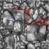 |
Fig. 1 Bolometric intensity map of the non-magnetic simulation of a field of view of 9.6 × 9.6 Mm2. The nMBP in the close-up on the left has a diameter of 80 km (resolved by approximately 8 × 8 computational cells). It has an intensity contrast of 35% with respect to the immediate neighbourhood but only 5% with respect to the global average intensity. A second nMBP is visible in the close-up on the lower right. Vertical sections along the blue lines in the close-up on the left are shown in Fig. 2. This figure is accompanied by a movie. |
Figure 1 shows two nMBPs in one of the intensity maps taken at t = 240 s after the relaxation phase of run Roe10. Like magnetic bright points, they are located in the intergranular space but are smaller in size. From the accompanying movie one can see that nMBPs appear in the intergranular space, often at vertices of intergranular lanes and they move with them or along intergranular lanes in a similar fashion to magnetic bright points. They often show a rotative proper motion.
Vertical sections of the density in planes along the lines of the blue cross indicated in Fig. 1 are shown in Fig. 2. In this figure, the blue curve indicates the optical depth unity for vertical lines of sight, which separates the convection zone from the photosphere. One notices that in the location of the nMBP, there is a funnel of reduced density (colour scale) that extends from the photosphere into the convection zone. The red curve indicates the local minimum of the density in horizontal planes. Similar funnels of low density are also found in connection with magnetic bright points. However, in the context of small-scale magnetic flux-tube models (see, e.g. Spruit 1976; Zwaan 1978; Steiner et al. 1986; Fisher et al. 2000; Steiner 2007) the pressure gradient caused by this low density region is balanced by the magnetic pressure of the magnetic field concentration.
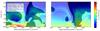 |
Fig. 2 Vertical sections through the nMBP shown in Fig. 1. The background colour shows mass density, where the brightness encodes the sign of the velocity perpendicular to the plane of projection: bright is plasma flowing out of the plane and dark is plasma flowing into it. The red curve indicates the spine of the nMBP, a “valley” in density, found as a sequence of local density minima in horizontal planes. The blue curve indicates the Rosseland optical depth unity. The legend gives intensity, density, and gas pressure contrast, firstly with respect to the neighbourhood and secondly with respect to the global average (at τ = 1 for the density and the pressure). |
The underlying mechanism causing nMBPs is necessarily different because no magnetic pressure is available. We can get information about this mechanism by looking at the Eulerian momentum equation 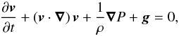 (1)where v is the velocity field, t the time, ρ the mass density, P the gas pressure, and g the gravitational acceleration at the solar surface. Assuming a stationary field we can neglect the first term. In a horizontal plane, gravity does not play any role, and therefore the pressure gradient can only be balanced by a particular shape of the velocity field, which appears in the advection term. In Fig. 2 the sign of the velocity field is encoded by means of brighter colours (velocity is going out of the plane of projection) and darker colours (velocity is going into it). Combining the information provided by the two planes, we conclude that plasma is swirling around the funnel of low density, the minimum of which is marked by the red curve.
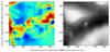 |
Fig. 3 Left: low-density regions in a sub-surface layer 200 km below ⟨τ⟩ = 1 sustaining swirls. The colour map extends from blue, indicating low density, to red, indicating high density, and the arrows represent the plasma velocity projected into the horizontal plane. Longest arrows correspond to a velocity of 9.5 km s-1. Such swirling low density regions are much more abundant than nMBPs but most of them do not extend into the photosphere and therefore do not produce nMBPs. Right: corresponding bolometric intensity map. Of the several low density swirling regions in the left panel only the one at (x,y) = (0,0) produces a nMBP. |
This swirling explains the stability of nMBPs only qualitatively, but it also provides insight into their formation. The plasma that rises to the photosphere by convection cools off, becomes denser, and subsequently sinks back into the convection zone in the intergranular lanes, which are smaller than the granules. Any small initial angular momentum in the plasma will lead, when downflows contract, to the generation of swirls. This effect has already been described by Nordlund (1985) in a slightly different context. There, it was referred as the “bath-tub” effect and appeared in the sub-surface layers at locations of downdrafting plumes. In our simulations we also find many locations with low densities in the sub-surface layers and corresponding swirls (see Fig. 3), but in general those swirls do not lead to bright points. In fact, bright points only appear if the low density funnel extends spatially from the convection zone to a significant height into the photosphere. Such an extended region of low density leads automatically to a depression of the unit optical depth isosurface (blue contour in Fig. 2), for which we will borrow the term “Wilson depression” in analogy to the observed depression in sunspots.
3. From a nMBP toy-model to a recognition algorithm
We now come back to the Eulerian momentum equation, Eq. (1). For establishing a toy model, we impose the following conditions, which derive from the properties of typical nMBPs, as the one shown in Figs. 1–3:
-
1.
nMBPs are long-lived and stable so that the velocity field can beconsidered stationary;
-
2.
they have cylindrical symmetry;
-
3.
their velocity field has a non-vanishing azimuthal component;
-
4.
they extend in the vertical direction and their shape does not depend on depth.
Because of the second assumption, the Euler momentum equation should be rewritten in cylindrical coordinates. The advection term is then given by ![Mathematical equation: \begin{eqnarray*} (\vect{v}\cdot\vect{\nabla})\vect{v}= \left[(\vect{v}\cdot\vect{\nabla})v_{r}- \frac{v_{\theta}^{2}}{r}\right]\vect{\hat{r}}+ \left[(\vect{v}\cdot\vect{\nabla})v_{\theta}+ \frac{v_{\theta}v_{r}\vphantom{v_{\theta}^{2}}}{r}\right] \vect{\hat{\theta}}+(\vect{v}\cdot\vect{\nabla})v_{z}\vect{\hat{z}}, \end{eqnarray*}](/articles/aa/full_html/2016/12/aa28649-16/aa28649-16-eq43.png) where the directional derivative is
where the directional derivative is  The simplest field satisfying the conditions 1–4 is
  Because of cylindrical symmetry, the pressure gradient is provided by
  . Inserting the velocity field into the Euler momentum equation and projecting it into the horizontal plane leads to the trivial statement that the pressure gradient is in fact provided by the centripetal force
  (2)When comparing the typical nMBPs of Figs. 1 and 2 to this model, it immediately turns out that assumptions 2 and 4 are only qualitatively fulfilled. The first assumption is less straight-forward; on the one hand, the dynamical timescale for nMBPs is
  and this timescale is in the order of seconds (6 ± 2 s in a 1000 × 1000 km2 neighbourhood around the nMBP of Fig. 1, on the τ = 1 isosurface). On the other hand, the simulations show nMBPs to have a typical lifespan in the order of the granulation timescale. The difference between the two timescales can in fact be expected when inspecting the simulations, because even though nMBPs exist for up to five minutes, they are moving, often even rotating, and their shape is continuously changing. The model could be refined by rewriting the velocity field as
  , where v0 is the bulk velocity of the nMBP and v′ is the stationary field that we have considered until now. We then get the new Euler momentum equation
  where, in general, v0 should also be a non-constant coordinate-dependent field. These considerations lead to the conclusion that no simple model can fully reproduce nMBPs’ behaviour. Nevertheless, the present toy model gives important insight into nMBPs and provides three correlated characteristics of them: (i) the presence of a pressure gradient, leading to a funnel of reduced density by virtue of the equation of state and therefore to a depression of the τ = 1 isosurface; (ii) the presence of swirling motion and with it vorticity in the velocity field; (iii) a local intensity contrast due to a temperature contrast at the location of the depressed τ = 1 isosurface. Based on this information, we have developed an algorithm by constructing an indicator (a growing function of pressure gradient, vorticity, and intensity contrast), and subsequent search of maxima of this indicator. More precisely, the steps are:
-
1.
Compute the indicator at τ = 1. We define hτ = 1 as the depth at which τ = 1, and ωv,z ≡ (∇ × v)z,τ = 1 the vertical component of the vorticity, and Tτ = 1 the temperature, all evaluated over the entire surface of τ = 1. Then, we define
 as a normalization operator applied to the array of values of each physical quantity, which linearly maps each value to a new value in the [0,1] interval. More precisely, given an array Aij,
  and the indicator function is then constructed empirically as
-
2.
Find the location of maxima of the indicator using a maximum filter (with sliding window of size 3 × 3).
-
3.
For each local maximum of the indicator, search in the intensity map for the closest intensity maximum. This defines the location of a candidate nMBP.
-
4.
Select granules (which we define as regions where the vertical velocity is positive at τ = 1) and intergranular lanes (complementary region).
-
5.
Select the intergranular, local neighbourhood in the intensity map for every candidate nMBP within an area of 100 × 100 computational cells centred on the nMBP. The boundary between the nMBP and the local neighbourhood is consistently defined to separate the region of intensity
 , the nMBP, from the region of intensity
  , the neighbourhood. Icentre is the maximal intensity in the nMBP region and Iout is the average intensity in the neighbourhood.
 -
6.
Select the spine of the nMBP in three-dimensional space. To keep the computational demand low, we first extract from the full computational domain a smaller box of 100 × 100 × 100 computational cells around its centre and the ⟨τ⟩ = 1 surface. Starting at the depth of τ = 1 in the centre of the nMBP and from there, layer by layer upwards and downwards, we look for local minima in the density. Exactly at τ = 1 we select the local density minimum closest to the approximate location of the nMBP as determined in step 3. For the adjacent layers, the selected local minimum is the one that is closest to that of the previous layer.
-
7.
Apply step 5 to scalar physical quantities other than the bolometric intensity, on either the z = 0 plane or the τ = 1 isosurface. Evaluate the local and global contrast of the corresponding scalar quantity (density, gas pressure, and temperature).
This algorithm managed very well to recognize all the nMBPs that we had previously selected by eye in an arbitrary snapshot. We then applied this algorithm to the entire time sequence of the simulation, producing similar plots as shown in Figs. 2 and 3. We have examined all the selected nMBPs visually and discarded those that were not properly selected (i.e. “twin” nMBPs that were very close to each other).
4. Physical properties of nMBPs
We investigate the following physical properties of nMBPs:
-
Equivalent
diameter
D
:
computed from the area A of a nMBP as determined in step 5 of the algorithm given in the previous section. Thus,
 .
. -
Wilson-depression
W
d
:
difference in height between the deepest point on the τ = 1 isosurface of a nMBP and the average height of this surface in the neighbourhood of the nMBP as determined in step 5 of the algorithm.
-
Intensity
contrast
C
I
:
computed locally and globally from CI ≡ (Ip−⟨I⟩)/⟨I⟩, where Ip is the average bolometric intensity of the nMBP and ⟨I⟩ is either the bolometric intensity averaged over the entire intensity map (global) or in the neighbourhood (local) of the nMBP as determined in step 5 of the algorithm.
-
Mass-density
contrast
C
ρ
:
computed locally and globally on the horizontal plane corresponding to ⟨τ⟩ = 1 (i.e., z = 0) and on the τ = 1 isosurface, respectively. As determined in step 7 of the algorithm, Cρ ≡ (ρ0−⟨ρ⟩)/⟨ρ⟩, where ρ0 is the minimal mass density inside the nMBP at the given surface and ⟨ρ⟩ is either the density averaged over the entire plane or in the neighbourhood at the given surface.
-
Pressure contrast
C
P
:
defined in the same way as the mass density contrast, with p0 taken at the same location as ρ0.
-
Temperature contrast
C
T
:
defined in the same way as the mass density and the pressure contrast, with T0 taken at the same location as ρ0.
-
Maximum
vertical velocity
 :
:
defined in the horizontal plane z = 0 (corresponding to ⟨τ⟩ = 1), inside the nMBP.
-
Maximum
horizontal velocity
 :
:
also defined in the horizontal plane z = 0 (corresponding to ⟨τ⟩ = 1), inside the nMBP.
-
Vorticity
ω
v,z
:
vertical component of the vorticity, defined in the horizontal plane z = 0 at the same location as ρ0.
-
Lifetime:
derived from a few nMBPs visually tracked on bolometric intensity maps of Roe10.
The nMBPs that enter the following statistics have been extracted from the two distinctly different magnetic field-free simulation runs Roe10 and Roe7 (see Table 1). The mean values and corresponding standard deviations of the physical quantities listed above (with the exception of the lifetime) are given in Table 2 for both simulation runs and (depending on the quantity) with respect to the plane at z = 0 and/or the τ = 1 surface and with respect to the local and global neighbourhood. For the lifetime, no automatic tracking of nMBPs was done because the cadence of 240 s of the full box data is not high enough. On the other hand, bolometric intensity maps are available at a high cadence of 10 s, but the tracking of nMBPs from the intensity maps alone would require involved pattern recognition techniques and criterions for the appearance and disappearance of nMBPs. Therefore we relied on a derivation from visually tracked nMBPs on the bolometric intensity maps. Qualitatively, we found bright points existing for a duration of 30 s up to the granular time-scale of a few min.
Physical quantities of nMBPs of two different simulations, Roe10 with a grid size of 10 km in every spatial direction and Roe7 with a grid size of 7 km in every direction.
For the first two entries in Table 2, the equivalent diameter D and the Wilson depression Wd, the corresponding histograms are given in Figs. 4 and 5, respectively. From Fig. 4 one readily sees that the diameters of nMBPs are distinctly smaller than those of magnetic bright points, which range from 100 km to 300 km according to Wiehr et al. (2004). The median value for the diameter is 78 km and 63 km for Roe10 and Roe7, respectively, while Wiehr et al. (2004) obtain 160 km for the most frequent diameter of magnetic bright points. In Fig. 4, one also observes that the distribution of diameters of Roe7 is rather sharply limited at 30 km and 95 km, which could suggest that nMBPs are about to be resolved in this simulation. Lowering the resolution can be expected to spread this distribution, which would then explain the apparition of wings in the size distribution of Roe10. But more likely, the low end of the distribution is given by the limited spatial resolution of the simulations. On the other hand, we cannot offer a plausible explanation for the extended wide wing to larger diameters in the histogram of Roe10.
Besides the physical quantities that appear on Table 2, another interesting quantity is the number of nMBPs per unit area, n10 and n7. We find n10 = 0.0712 Mm-2 and n7 = 0.189 Mm-2, which indicates that at higher spatial resolution, we observe more than twice as many bright points than at lower resolution. The histograms of Figs. 4 and 5 are normalized to these respective number densities. The histogram of the equivalent diameter shown in Fig. 4 suggests that this surplus is due to a larger number of small bright points detected at higher spatial resolution. However, there still remains a difference of a factor of two between number densities in the two simulations when restricting statistical analyses to nMBPs larger than 60 km in diameter; a value that is significantly greater than the spatial resolution of both simulations. This suggests that the high resolution simulation not only harbours more small and tiny nMBPs but also greatly favours the formation of large nMBPs.
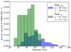 |
Fig. 4 Size distribution of nMBPs, normalized to the average number density in the corresponding simulation. |
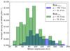 |
Fig. 5 Distribution of the Wilson-depression of nMBPs, normalized to the average number density in the corresponding simulation. |
The distribution of the Wilson depression, given in Fig. 5, also shows an interesting trend: in the higher resolution model Roe7, it is globally shifted towards smaller depths compared to the distribution from Roe10. An intuitive explanation for this fact would be a correlation between size and Wilson depression, which, however, does not exist. There are a number of numerical parameters that differ between simulations Roe10 and Roe7 but numerous test runs confirmed that none of these seem to substantially influence the Wilson depression. We therefore found no convincing explanation why simulation Roe7 shows nMBPs to have a mean Wilson depression which is approximately 20 km less than that of simulation Roe10. In any case, the Wilson depression of nMBPs of respectively 103 km and 83 km for Roe10 and Roe7 is again clearly smaller than corresponding values for magnetic bright points of, typically, 150 km (Salhab et al., in prep.).
In Table 2, one can see that the average values of contrasts of intensity, mass density, pressure, and temperature do not differ substantially between the two simulations. At first, this seems to be at odds with the fact that the Wilson depression is larger in Roe10 compared to Roe7. Thinking of a plane-parallel, exponentially-stratified, hydrostatic atmosphere one would expect the density contrast at τ = 1 to also be larger in Roe10 compared to Roe7. However, this is only partially the case. The reason is that close to τ = 1, the density runs rather constant with height due to the onset of radiative loss and a corresponding sharp drop in temperature (this is the quasi density reversal that causes the Rayleigh-Taylor instability that drives the convection). Furthermore, the funnel-shaped structure of the nMBPs accentuates this behavior; smaller radii in deeper layers go together with faster swirling motion that can sustain larger gradients in mass density and pressure, which counteracts stratification of the atmosphere inside the nMBP. The absence of exponential stratification then keeps the density contrast insensitive to the Wilson depression.
 |
Fig. 6 Vertical section through a typical nMBP showing isotherms (labeled coloured curves) and the mass density plotted in the background (light is low density and dark blue is high density). The τ = 1 isosurface is the dashed red curve. This surface intersects the isotherms, reaching to high temperatures where it dips deep down at the location of the nMBP at x ≈ 8100 km. |
The intensity contrast (third entry in Table 2) is a quantity that can be directly observed. As is the case for the contrast of temperature at the τ = 1 isosurface, its value drastically depends on whether it is evaluated locally (with respect to the local neighbourhood) or globally (with respect to the mean intensity/temperature). This is due to the fact that nMBPs are formed within the dark intergranular space and are, compared to granules, not so bright. Some of the nMBPs are even darker than the average intensity over the whole bolometric map, but they are still conspicuous objects within the dark intergranular lanes (see also Title & Berger 1996, for the same effect in the context of magnetic bright points). The contrast of the bolometric intensity of nMBPs in the order of 20% (local) and 0% (global) is again distinctively smaller than the measured global continuum contrast of magnetic bright points at 588 nm of 10% to 15% by Wiehr et al. (2004) and at 525 nm of 37% (local) and 11% (global) by Riethmüller et al. (2010). We ascribe this difference to the difference in the formation of magnetic bright points and nMBPs. Magnetic flux tubes are prone to the convective collapse instability (Spruit 1979), which leads to a high degree of evacuation and with it to a large Wilson depression and intensity contrast. No such instability and evacuation takes place in the case of nMBPs. Like Wiehr et al. (2004) for magnetic bright points, we do not find a correlation between local intensity contrast and effective diameter of nMBPs.
The temperature contrast on the isosurface of unit optical depth is positive as can be seen from Table 2. This can be seen in Fig. 6, which shows that isotherms intersect the τ = 1 isosurface, similarly to magnetic bright points (see, e.g. Fig. 2 of Steiner 2007). It is interesting to note that isotherms generally also have a depression at the location of the nMBP funnel, although smaller than the depression of optical depth unity. This can be expected because of the swirling downdraft of cool photospheric material at locations of nMBPs. The temperature contrast on a horizontal plane of constant geometrical depth can therefore be negative, although it is always positive on the τ = 1 isosurface, which is also the reason for the brightness of nMBPs. Pressure and density contrasts have very similar values, which is expected because both quantities are related by the equation of state, while the temperature contrast is relatively low. The nMBPs form in swirling downdrafts in the intergranular space. The maximal vertical velocity ranging from 5.5 to 7 km s-1 approaches sonic speed.
The vertical vortex event described by Moll et al. (2011) has a diameter of 80 km, a Wilson depression of 110 km, an intensity contrast of 0.24, and global density and pressure contrasts at z = 0 of − 0.64. This is one example observed in a simulation with a grid size of 4 × 4 × 4 km3 as obtained with the MURaM code (Vögler et al. 2005). These values are in closeagreement with the values and standard deviations given in Table 2 suggesting that this vortex event is of the same class of objects described herein. Correspondingly, we can consider nMBPs to be manifestations of vertically extending vortex tubes, which themselves are the manifestation of the turbulent nature of the near surface convection.
Regarding the horizontal, azimuthal velocities in nMBPs, the toy model in Sect. 3 provides an order of magnitude estimate. For this, we consider the relations  where P, ρ, Cρ, T, CT, Teff and vθ stand for gas pressure, mass density, density contrast, temperature, temperature contrast, effective temperature, and tangential velocity respectively, and Rs is the specific gas constant for which we choose the mean molecular weight μ = 1.224. The indices “int” and “ext” refer to the centre of the nMBP funnel and to its close surrounding, respectively, always in the horizontal plane of ⟨τ⟩ = 1. The first equation is derived from Eq. (2). One can then express the tangential velocity as a function of density contrast, temperature contrast, and effective temperature as
 ![Mathematical equation: \begin{eqnarray*} v_{\theta}=\sqrt{R_{\mathrm{s}}\,T_{\mathrm{eff}} \left[1-(1+C_{\rho})(1+C_{T})\right]} \approx\sqrt{\frac{R_{\mathrm{s}}\,T_{\mathrm{eff}}}{2}}=4.4\, \mbox{km}\,\mbox{s}^{-1}\,. \end{eqnarray*}](/articles/aa/full_html/2016/12/aa28649-16/aa28649-16-eq124.png) Here, we used Cρ ≈ −0.5 and CT ≈ 0 from Table 2, referring to the horizontal plane ⟨τ⟩ = 1. This value is approximately half the actual maximal horizontal velocity of nMBPs in the simulations, which is, close to nMBP centres, around 9–9.5 km s-1 according to Table 2.
Here, we used Cρ ≈ −0.5 and CT ≈ 0 from Table 2, referring to the horizontal plane ⟨τ⟩ = 1. This value is approximately half the actual maximal horizontal velocity of nMBPs in the simulations, which is, close to nMBP centres, around 9–9.5 km s-1 according to Table 2.
As expected, there are as many bright points rotating clockwise as there are rotating anti-clockwise. We verified that the average value of the vertical component of the vorticity ⟨ωv,z⟩ is indeed close to zero.
Using both the Eddington-Barbier relation and the Stefan-Boltzmann law, the temperature contrast at τ = 1 and the intensity contrast are related as  It is verified in the simulations that
  and the Pearson cross-correlation coefficient for these two contrasts is given by ρ = 0.49 (Roe10 simulation) and ρ = 0.35 (Roe7 simulation).
5. nMBPs in intensity maps of virtual observations
The kind of nMBPs described here have not been observed with currently operating solar telescopes, presumably because of their small size and relatively low intensity contrast. Non-magnetic photospheric bright points have been reported to exist by Berger & Title (2001) and by Langhans et al. (2002). However, those bright points exist on the edges of certain bright, rapidly expanding granules while nMBPs are located within intergranular lanes. The objects reported by Berger & Title (2001) and by Langhans et al. (2002) are probably identical with the bright grains that often appear with the development of granular lanes (Yurchyshyn et al. 2011).
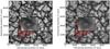 |
Fig. 7 Single snapshot of the Roe10 simulation showing the intensity in the continuum at 5000 Å (left) and the corresponding degraded image with a GREGOR-like point-spread function (right). A typical nMBP of 80 km diameter is magnified. |
The present bright points are non-magnetic by construction, and it is therefore unclear to what extent such bright points really exist in the solar photosphere that is virtually ubiquitously occupied by magnetic fields (Lites et al. 2008). In reality, the pressure gradient that is at the origin of nMBPs is probably always provided by a combination of the centripetal force and the magnetic pressure gradient, however, in regions of low magnetic flux, it may happen that the pressure gradient results mainly from the swirling motion.
In order to gain insight into the requirements for the observational detection of nMBPs, we have degraded our synthetic intensity maps to simulate observations with existing solar telescopes, such as the 50 cm Solar Optical Telescope (SOT) aboard the Hinode space observatory (Tsuneta et al. 2008), the 1 m telescope aboard the Sunrise balloon-borne solar observatory (Barthol et al. 2011), and the 1.5 m ground-based GREGOR solar telescope (Schmidt et al. 2012), as well as with future solar telescopes currently under construction, such as the 4 m Daniel K. Inouye Solar Telescope (DKIST; Keil et al. 2010), or planned solar telescopes such as the space-borne 1.5 m Solar UV-Visible-IR Telescope (SUVIT; Suematsu et al. 2014), the 2 m Indian National Large Solar Telescope (NLST; Hasan et al. 2010), and the 4 m European Solar Telescope (EST; Collados et al. 2010). The point spread functions (PSFs) that we have constructed are convolutions of the diffraction-limited PSFs, taking the entrance pupil (including secondary mirror and spider) of the various instruments into account, with Lorentz functions. The Lorentz functions are intended to account for non-ideal contributions due to stray-light inside the instrument. Their γ parameter has been chosen to inversely scale with the telescope aperture, with the reference value for the 50 cm SOT aperture given by the greatest value deduced by Wedemeyer-Böhm (2008) from observations of the Mercury transit from 2006 and the solar eclipse from 2007. Wedemeyer-Böhm (2008) has carried out convolutions with both Voigt and Lorentz functions in different observational situations. Unfortunately, the optimal parameters are quite sensitive to observational scenarios. We have thus decided to retain as few parameters as possible (choosing the Lorentz function over the Voigt function) and we also chose γ = 9, when different situations suggest a range of values from 7 ± 1 up to 9 ± 1. Our PSFs are therefore more realistic than simple diffraction-limited PSFs but are nonetheless not fully accurate.
According to Fig. 7, nMBPs could be seen using the GREGOR solar telescope. However, the spatial resolution capability of GREGOR of  at 500 nm corresponds to ≈60 km on the Sun, so that an 80 km nMBP would appear as a brightness enhancement in one single resolution element only. Furthermore, to be sure that the nMBP harbours no strong magnetic field, a simultaneous polarimetric measurement needs to be carried out, for which the resolution is a mere
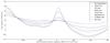 |
Fig. 8 Intensity contrast in the continuum at 5000 Å across the nMBP of Fig. 7 (section along y-axis), using degraded images obtained with a variety of PSFs that correspond to the solar telescopes listed in the text. The legend orders the telescopes according to the simulated peak contrast, from highest to lowest. The curves with degradations corresponding to DKIST and EST are close to congruent. The coordinate x = 0 corresponds to the centre of the nMBP, which is taken to be the point of lowest density in the τ = 1 isosurface. Note that the peak intensity is displaced with respect to this nMBP centre because the nMBP funnel is inclined with respect to the vertical direction, as is often the case, such as that visible in the right-hand panel of Fig. 2. |
From Fig. 8 one can see that the peak intensity observed in telescopes with apertures up to 2 m is barely higher than the intensity in the immediate vicinity, and the nMBP appears larger than in the raw simulations, making it very difficult to distinguish it from other bright structures.
From this, we conclude that telescopes with large apertures, such as DKIST or EST, are needed to approach the contrast of nMBPs found in the simulations and in order to achieve sufficiently high spatial resolution in polarimetry for an unambiguous detection of nMBPs.
6. Conclusion
This paper investigates bright points that appear within intergranular lanes of high-resolution, magnetic field-free, numerical simulations of the solar photosphere. The most striking properties of these features are that on the τ = 1 isosurface, their temperature is, on average, 5% higher than the mean temperature (which makes them appear bright), their mass density is lower in a funnel extending from the upper convection zone to the lower photosphere, and they comprise transonic swirling motions. At the location of the bright point, the τ = 1 isosurface lies, on average, 80−100 km deeper than the horizontal plane z = 0 (corresponding to the mean optical depth ⟨τ⟩ = 1). At this level (z = 0), their density and pressure are reduced by approximately 60% of the corresponding global average values at the same level. On average, their size (equivalent diameter) is approximately 60−80 km, corresponding to 0.̋08−0.̋11, and their bolometric intensity contrast is approximately 20% with respect to their immediate intergranular surroundings. The number of nMBPs per unit area is 0.07–0.19 Mm-2 and their lifespan ranges from approximately 30 s up to the granular lifetime of several minutes.
Based on some of these properties an algorithm for the automatic detection of nMBPs has been developed that enables us to derive statistics of their physical properties. Comparing the statistics of two simulations with differing spatial resolutions of 10 km and 7 km, we find nMBP equivalent diameters down to the resolution limit of the simulations. At the upper end of the size distribution, we find twice as many bright points with the higher spatial resolution as we do with the lower spatial resolution. Also, we find that in subsurface layers, swirling low density funnels are much more abundant than nMBPs. These low density funnels appear only as bright points under the condition that they extend into the photosphere. The characteristics of the nMBPs found here are in close agreement with corresponding properties of vertical vortices found by Moll et al. (2011). Thus, nMBPs are an observable manifestation of vertically directed vortex tubes, similar to bright granular lanes, which are a manifestation of horizontally directed vortex tubes (Steiner et al. 2010).
Both nMBPs and granular lanes together offer a glimpse of the elements of turbulence at work in a stratified medium, which is of basic physical interest. The nMBPs are so minuscule that they seem not to have any impact on the overall appearance of granules and the near surface convection. However, as soon as magnetic flux concentrations are attracted by and caught into the swirling down draft of a nMBP, we expect them to have a major impact on the tenuous atmosphere higher up through magnetic coupling (Shelyag et al. 2011; Steiner & Rezaei 2012). Chromospheric swirls (Wedemeyer-Böhm & Rouppe van der Voort 2009) and magnetic tornadoes (Wedemeyer-Böhm et al. 2012; Wedemeyer & Steiner 2014) would be the consequences.
Such nMBPs are barely detectable using currently operating solar telescopes because of their small size and relatively low contrast, and due to the limited spatial resolution of the magnetograms achievable with these telescopes (currently ≈ . High-resolution magnetograms are needed to prove the absence of strong magnetic fields in nMBPs. If nMBPs exist, they should be observable with the new generation of 4-m-class telescopes in regions of very weak magnetic fields. The Visible Tunable Filter (VTF; Schmidt et al. 2014) of DKIST is designed to produce diffraction-limited magnetograms, which should therefore be adequate for the unambiguous detection of nMBPs.
Online material
Movie of Fig. 1 Access Supplementary Material
Acknowledgments
This work was supported by the Swiss National Science Foundation under grant ID 200020_157103/1 and by a grant from the Swiss National Supercomputing Centre (CSCS) in Lugano under project ID s560. The numerical simulations were carried out at CSCS on the machines named Rothorn and Piz Dora. Model d3t57g44b0 was computed at the Pôle Scientifique de Modélisation Numérique (PSMN) at the École Normale Supérieure (ENS) in Lyon. Special thanks are extended to S. Wedemeyer for help with the PSF and to the anonymous referee for very helpful comments.
References
- Barthol, P., Gandorfer, A., Solanki, S. K., et al. 2011, Sol. Phys., 268, 1 [NASA ADS] [CrossRef] [Google Scholar]
- Beeck, B., Cameron, R. H., Reiners, A., & Schüssler, M. 2013, A&A, 558, A49 [NASA ADS] [CrossRef] [EDP Sciences] [Google Scholar]
- Beeck, B., Schüssler, M., Cameron, R. H., & Reiners, A. 2015,A&A, 581, A43 [Google Scholar]
- Berger, T. E., & Title, A. M. 1996, ApJ, 463, 365 [NASA ADS] [CrossRef] [Google Scholar]
- Berger, T. E., & Title, A. M. 2001, ApJ, 553, 449 [NASA ADS] [CrossRef] [Google Scholar]
- Berger, T. E., Rouppe van der Voort, L. H. M., Löfdahl, M. G., et al. 2004, A&A, 428, 613 [NASA ADS] [CrossRef] [EDP Sciences] [Google Scholar]
- Carlsson, M., Stein, R. F., Nordlund, Å., & Scharmer, G. B. 2004, ApJ, 610, L137 [NASA ADS] [CrossRef] [Google Scholar]
- Collados, M., Bettonvil, F., Cavaller, L., et al. 2010, Astron. Nachr., 331, 615 [NASA ADS] [CrossRef] [Google Scholar]
- Dunn, R. B., & Zirker, J. B. 1973, Sol. Phys., 33, 281 [NASA ADS] [Google Scholar]
- Fisher, G. H., Fan, Y., Longcope, D. W., Linton, M. G., & Pevtsov, A. A. 2000, Sol. Phys., 192, 119 [NASA ADS] [CrossRef] [Google Scholar]
- Freytag, B. 2013, Mem. Soc. Astron. It. Suppl., 24, 26 [Google Scholar]
- Freytag, B., Steffen, M., Ludwig, H.-G., et al. 2012, J. Comput. Phys., 231, 919 [Google Scholar]
- Hasan, S. S., Soltau, D., Kärcher, H., Süss, M., & Berkefeld, T. 2010, in Ground-based and Airborne Telescopes III, Proc. SPIE, 7733, 77330I [CrossRef] [Google Scholar]
- Keil, S. L., Rimmele, T. R., Wagner, J., & ATST Team 2010, Astron. Nachr., 331, 609 [NASA ADS] [CrossRef] [Google Scholar]
- Keller, C. U., Schüssler, M., Vögler, A., & Zakharov, V. 2004, ApJ, 607, L59 [NASA ADS] [CrossRef] [Google Scholar]
- Langhans, K., Schmidt, W., & Tritschler, A. 2002, A&A, 394, 1069 [NASA ADS] [CrossRef] [EDP Sciences] [Google Scholar]
- Lites, B. W., Kubo, M., Socas-Navarro, H., et al. 2008, ApJ, 672, 1237 [NASA ADS] [CrossRef] [Google Scholar]
- Mehltretter, J. P. 1974, Sol. Phys., 38, 43 [NASA ADS] [CrossRef] [Google Scholar]
- Moll, R., Cameron, R. H., & Schüssler, M. 2011, A&A, 533, A126 [NASA ADS] [CrossRef] [EDP Sciences] [Google Scholar]
- Moll, R., Cameron, R. H., & Schüssler, M. 2012, A&A, 541, A68 [NASA ADS] [CrossRef] [EDP Sciences] [Google Scholar]
- Muller, R., & Roudier, T. 1984, Sol. Phys., 94, 33 [NASA ADS] [CrossRef] [Google Scholar]
- Nordlund, A. 1985, Sol. Phys., 100, 209 [NASA ADS] [CrossRef] [Google Scholar]
- Nordlund, Å., Stein, R. F., & Asplund, M. 2009, Liv. Rev. Sol. Phys., 6 [Google Scholar]
- Riethmüller, T. L., Solanki, S. K., Martínez Pillet, V., et al. 2010, ApJ, 723, L169 [NASA ADS] [CrossRef] [Google Scholar]
- Roe, P. L. 1986, Ann. Rev. Fluid Mech., 18, 337 [NASA ADS] [CrossRef] [Google Scholar]
- Sánchez Almeida, J., Asensio Ramos, A., Trujillo Bueno, J., & Cernicharo, J. 2001, ApJ, 555, 978 [NASA ADS] [CrossRef] [Google Scholar]
- Schmidt, W., von der Lühe, O., Volkmer, R., et al. 2012, Astron. Nachr., 333, 796 [NASA ADS] [CrossRef] [Google Scholar]
- Schmidt, W., Bell, A., Halbgewachs, C., et al. 2014, in Ground-based and Airborne Instrumentation for Astronomy V, Proc. SPIE, 9147, 91470E [CrossRef] [Google Scholar]
- Schüssler, M., Shelyag, S., Berdyugina, S., Vögler, A., & Solanki, S. K. 2003, ApJ, 597, L173 [NASA ADS] [CrossRef] [Google Scholar]
- Shelyag, S., Schüssler, M., Solanki, S. K., Berdyugina, S. V., & Vögler, A. 2004, A&A, 427, 335 [NASA ADS] [CrossRef] [EDP Sciences] [Google Scholar]
- Shelyag, S., Keys, P., Mathioudakis, M., & Keenan, F. P. 2011, A&A, 526, A5 [NASA ADS] [CrossRef] [EDP Sciences] [Google Scholar]
- Spruit, H. C. 1976, Sol. Phys., 50, 269 [NASA ADS] [CrossRef] [Google Scholar]
- Spruit, H. C. 1979, Sol. Phys., 61, 363 [NASA ADS] [CrossRef] [Google Scholar]
- Stein, R. F. 2012, Philos. Trans. Roy. Soc. London Ser., A, 370, 3070 [Google Scholar]
- Steiner, O. 2005, A&A, 430, 691 [NASA ADS] [CrossRef] [EDP Sciences] [Google Scholar]
- Steiner, O. 2007, in Kodai School on Solar Physics, eds. S. S. Hasan, & D. Banerjee, AIP Conf. Ser., 919, 74 [Google Scholar]
- Steiner, O., & Rezaei, R. 2012, in Fifth Hinode Science Meeting, eds. L. Golub, I. De Moortel, & T. Shimizu, ASP Conf. Ser., 456, 3 [Google Scholar]
- Steiner, O., Pneuman, G. W., & Stenflo, J. O. 1986, A&A, 170, 126 [NASA ADS] [Google Scholar]
- Steiner, O., Hauschildt, P. H., & Bruls, J. 2001, A&A, 372, L13 [NASA ADS] [CrossRef] [EDP Sciences] [Google Scholar]
- Steiner, O., Franz, M., Bello González, N., et al. 2010, ApJ, 723, L180 [NASA ADS] [CrossRef] [Google Scholar]
- Suematsu, Y., Katsukawa, Y., Hara, H., et al. 2014, in Space Telescopes and Instrumentation 2014: Optical, Infrared, and Millimeter Wave,Proc. SPIE, 9143, 91431 [Google Scholar]
- Title, A. M., & Berger, T. E. 1996, ApJ, 463, 797 [NASA ADS] [CrossRef] [Google Scholar]
- Tsuneta, S., Ichimoto, K., Katsukawa, Y., et al. 2008, Sol. Phys., 249, 167 [NASA ADS] [CrossRef] [Google Scholar]
- Utz, D., del Toro Iniesta, J. C., Bellot Rubio, L. R., et al. 2014, ApJ, 796, 79 [NASA ADS] [CrossRef] [Google Scholar]
- Vögler, A., Shelyag, S., Schüssler, M., et al. 2005, A&A, 429, 335 [NASA ADS] [CrossRef] [EDP Sciences] [Google Scholar]
- Wedemeyer, S., & Steiner, O. 2014, PASJ, 66, S10 [NASA ADS] [CrossRef] [Google Scholar]
- Wedemeyer-Böhm, S. 2008, A&A, 487, 399 [NASA ADS] [CrossRef] [EDP Sciences] [Google Scholar]
- Wedemeyer-Böhm, S., & Rouppe van der Voort, L. 2009, A&A, 507, L9 [NASA ADS] [CrossRef] [EDP Sciences] [Google Scholar]
- Wedemeyer-Böhm, S., Scullion, E., Steiner, O., et al. 2012, Nature, 486, 505 [NASA ADS] [CrossRef] [PubMed] [Google Scholar]
- Wiehr, E., Bovelet, B., & Hirzberger, J. 2004, A&A, 422, L63 [NASA ADS] [CrossRef] [EDP Sciences] [Google Scholar]
- Yurchyshyn, V. B., Goode, P. R., Abramenko, V. I., & Steiner, O. 2011, ApJ, 736, L35 [NASA ADS] [CrossRef] [Google Scholar]
- Zwaan, C. 1978, Sol. Phys., 60, 213 [Google Scholar]
All Tables
Box and cell sizes, number of opacity bands, nopbds, and run duration, trun, for the two simulation runs Roe10 (d3t57g45b0roefc) and Roe7 (d3t57g44b0).
Physical quantities of nMBPs of two different simulations, Roe10 with a grid size of 10 km in every spatial direction and Roe7 with a grid size of 7 km in every direction.
All Figures
|
Fig. 1 Bolometric intensity map of the non-magnetic simulation of a field of view of 9.6 × 9.6 Mm2. The nMBP in the close-up on the left has a diameter of 80 km (resolved by approximately 8 × 8 computational cells). It has an intensity contrast of 35% with respect to the immediate neighbourhood but only 5% with respect to the global average intensity. A second nMBP is visible in the close-up on the lower right. Vertical sections along the blue lines in the close-up on the left are shown in Fig. 2. This figure is accompanied by a movie. |
| In the text | |
|
Fig. 2 Vertical sections through the nMBP shown in Fig. 1. The background colour shows mass density, where the brightness encodes the sign of the velocity perpendicular to the plane of projection: bright is plasma flowing out of the plane and dark is plasma flowing into it. The red curve indicates the spine of the nMBP, a “valley” in density, found as a sequence of local density minima in horizontal planes. The blue curve indicates the Rosseland optical depth unity. The legend gives intensity, density, and gas pressure contrast, firstly with respect to the neighbourhood and secondly with respect to the global average (at τ = 1 for the density and the pressure). |
| In the text | |
|
Fig. 3 Left: low-density regions in a sub-surface layer 200 km below ⟨τ⟩ = 1 sustaining swirls. The colour map extends from blue, indicating low density, to red, indicating high density, and the arrows represent the plasma velocity projected into the horizontal plane. Longest arrows correspond to a velocity of 9.5 km s-1. Such swirling low density regions are much more abundant than nMBPs but most of them do not extend into the photosphere and therefore do not produce nMBPs. Right: corresponding bolometric intensity map. Of the several low density swirling regions in the left panel only the one at (x,y) = (0,0) produces a nMBP. |
| In the text | |
|
Fig. 4 Size distribution of nMBPs, normalized to the average number density in the corresponding simulation. |
| In the text | |
|
Fig. 5 Distribution of the Wilson-depression of nMBPs, normalized to the average number density in the corresponding simulation. |
| In the text | |
|
Fig. 6 Vertical section through a typical nMBP showing isotherms (labeled coloured curves) and the mass density plotted in the background (light is low density and dark blue is high density). The τ = 1 isosurface is the dashed red curve. This surface intersects the isotherms, reaching to high temperatures where it dips deep down at the location of the nMBP at x ≈ 8100 km. |
| In the text | |
|
Fig. 7 Single snapshot of the Roe10 simulation showing the intensity in the continuum at 5000 Å (left) and the corresponding degraded image with a GREGOR-like point-spread function (right). A typical nMBP of 80 km diameter is magnified. |
| In the text | |
|
Fig. 8 Intensity contrast in the continuum at 5000 Å across the nMBP of Fig. 7 (section along y-axis), using degraded images obtained with a variety of PSFs that correspond to the solar telescopes listed in the text. The legend orders the telescopes according to the simulated peak contrast, from highest to lowest. The curves with degradations corresponding to DKIST and EST are close to congruent. The coordinate x = 0 corresponds to the centre of the nMBP, which is taken to be the point of lowest density in the τ = 1 isosurface. Note that the peak intensity is displaced with respect to this nMBP centre because the nMBP funnel is inclined with respect to the vertical direction, as is often the case, such as that visible in the right-hand panel of Fig. 2. |
| In the text | |
Current usage metrics show cumulative count of Article Views (full-text article views including HTML views, PDF and ePub downloads, according to the available data) and Abstracts Views on Vision4Press platform.
Data correspond to usage on the plateform after 2015. The current usage metrics is available 48-96 hours after online publication and is updated daily on week days.
Initial download of the metrics may take a while.