| Issue |
A&A
Volume 595, November 2016
|
|
|---|---|---|
| Article Number | A11 | |
| Number of page(s) | 11 | |
| Section | Stellar atmospheres | |
| DOI | https://doi.org/10.1051/0004-6361/201628825 | |
| Published online | 24 October 2016 | |
Fine structure of the age-chromospheric activity relation in solar-type stars
I. The Ca II infrared triplet: Absolute flux calibration⋆,⋆⋆
1 Observatório do Valongo, Universidade Federal do Rio de Janeiro, Ladeira do Pedro Antonio 43, CEP: 20080-090 Rio de Janeiro, RJ, Brazil
e-mail: This email address is being protected from spambots. You need JavaScript enabled to view it.
; This email address is being protected from spambots. You need JavaScript enabled to view it.
; This email address is being protected from spambots. You need JavaScript enabled to view it.
2 Institut de Ciències de l’Espai (CSIC-IEEC), Facultat de Ciències, Carrer de Can Magrans, s/n, Campus UAB, 08193 Bellaterra, Spain
e-mail: This email address is being protected from spambots. You need JavaScript enabled to view it.
3 Departamento de Física Teórica e Experimental, Universidade Federal do Rio Grande do Norte, Campus Universitário Lagoa Nova, 59072-970 Natal, RN, Brazil
e-mail: This email address is being protected from spambots. You need JavaScript enabled to view it.
Received: 29 April 2016
Accepted: 7 June 2016
Abstract
Context. Strong spectral lines are useful indicators of stellar chromospheric activity. They are physically linked to the convection efficiency, differential rotation, and angular momentum evolution and are a potential indicator of age. However, for ages > 2 Gyr, the age-activity relationship remains poorly constrained thus hampering its full application.
Aims. The Ca II infrared triplet (IRT lines, λλ 8498, 8542, and 8662) has been poorly studied compared to classical chromospheric indicators. We report in this paper absolute chromospheric fluxes in the three Ca II IRT lines, based on a new calibration tied to up-to-date model atmospheres.
Methods. We obtain the Ca II IRT absolute fluxes for 113 FGK stars from high signal-to-noise ratio (S/N) and high-resolution spectra covering an extensive domain of chromospheric activity levels. We perform an absolute continuum flux calibration for the Ca II IRT lines anchored in atmospheric models calculated as an explicit function of effective temperatures (Teff), metallicity ([Fe/H]), and gravities (log g) avoiding the degeneracy usually present in photometric continuum calibrations based solely on color indices.
Results. The internal uncertainties achieved for continuum absolute flux calculations are ≈2% of the solar chromospheric flux, one order of magnitude lower than for photometric calibrations. Using Monte Carlo simulations, we gauge the impact of observational errors on the final chromospheric fluxes due to the absolute continuum flux calibration and find that Teffuncertainties are properly mitigated by the photospheric correction leaving [Fe/H] as the dominating factor in the chromospheric flux uncertainty.
Conclusions. Across the FGK spectral types, the Ca II IRT lines are sensitive to chromospheric activity. The reduced internal uncertainties reported here enable us to build a new chromospheric absolute flux scale and explore the age-activity relation from the active regime down to very low activity levels and a wide range of Teff, mass, [Fe/H], and age.
Key words: stars: atmospheres / stars: chromospheres / stars: late-type / solar neighborhood / techniques: spectroscopic / stars: activity
Based on spectroscopic observations collected at the Observatório do Pico dos Dias (OPD), operated by the Laboratório Nacional de Astrofísica, CNPq, Brazil, and the European Southern Observatory (ESO), within the ON/ESO and ON/IAG agreements, under FAPESP project No. 1998/10138-8.
Full Table 1 is only available at the CDS via anonymous ftp to cdsarc.u-strasbg.fr (130.79.128.5) or via http://cdsarc.u-strasbg.fr/viz-bin/qcat?J/A+A/595/A11
© ESO, 2016
1. Introduction
The seminal work of Skumanich (1972) established that stellar rotation in solar-type stars decays rapidly with age. The paradigm states that as an isolated star ages it loses a fraction of its mass through coronal winds. The mass loss leads consequently to a decrease in the angular momentum and the torque acts on the stellar surface slowing the rotation over millions of years. As a result, the stellar rotation braking causes a lower efficiency in the generation and amplification of magnetic fields at the base of the convective zone (Parker 1970) and less chromospheric heating (Noyes et al. 1984). As an observational indication of this effect, the profiles of strong spectral lines such as Ca II H & K, infrared triplet lines, Hα, and other chromospheric indicators respond to changes in the temperature distribution at high atmospheric altitudes showing a reduced core chromospheric signature as the star ages.
A number of empirical studies have attempted to convert the observed level of chromospheric emission into physical units (Hall et al. 2007, and references therein). This process enables a broad astrophysical interpretation of the chromospheric activity phenomena across a wide range of masses, ages, chemical compositions, and evolutionary states. The possibility of age-activity calibrations as well as their connections to rotational evolution, the properties of exoplanetary host stars, and chemodynamical evolution of the Galaxy turns the chromospheric activity estimates into important physical variables. In order to explore the nature of the chromospheric activity evolution, strong spectral features are commonly used.
The lines of the Ca II infrared triplet at 8498.062 (T1), 8542.144 (T2), and 8662.170 (T3) Å are formed in the lower chromosphere by subordinate transitions between the excited levels of Ca II 42P1/2,3/2 and meta-stable 32D3/2,5/2. This characteristic increases the opacity turning these spectral lines very intense and probing the physical conditions of a large range of atmospheric layers (Mihalas 1978). Physically, it is expected that the chromospheric radiative losses of Ca II lines (Ca II IRT and H & K) be strongly related because they share the same upper excited state (42P1/2,3/2) (Linsky et al. 1979b). The consequence of the coupling is that these Ca II lines are mostly collisionally controlled in the lower chromosphere and very sensitive to the local temperature (Cauzzi et al. 2008). For these reasons, the Ca II IRT is studied as an indicator of chromospheric activity (Linsky et al. 1979a; Foing et al. 1989; Chmielewski 2000; Busà et al. 2007) revealing itself as an interesting alternative for solar-type chromospheres studies and angular momentum evolution (Krishnamurthi et al. 1998). These lines show attractive intrinsic characteristics such as:
-
1.
The stellar continuum in λλ 8400−8800 is barely affected by telluric lines (Busà et al. 2007; Dempsey et al. 1993) and has a smaller density of photospheric lines which favors a more consistent spectra normalization and absolute continuum calibration of FGK stars in comparison to λλ 3900−4000. Furthermore, the theoretical flux distribution in the visible and infrared regions are better determined when compared to shorter wavelengths (Edvardsson 2008).
-
2.
The profile of Ca II IRT lines (especially the wings) is sensitive to macroscopic fundamental parameters such as Teff, [Fe/H], and log g(Andretta et al. 2005). These lines are important in the context of Galactic and extragalactic chemical enrichment as they allow the determination of Ca abundances or the estimation of [α/Fe] in M dwarfs (Terrien et al. 2015).
-
3.
Late-K and M stars have its flux distribution peaked towards longer wavelengths making the observation of visible and near-infrared chromospheric indicators such as Hα and Ca II IRT easier when compared to UV counterparts like Ca II H & K lines.
-
4.
Their less pronounced contrast compared to other classical chromospheric indicators makes the Ca II IRT more suitable for the measurement of the stellar mean activity level since they are less sensitive to sudden modulations caused by flares and transient phenomena.
A notorious disadvantage of the IRT lines is the lower instrumental contrast between the chromospheric and photospheric contributions compared to Hα and H & K lines, demanding spectra of good quality and a careful analysis of inactive stars. Moreover, (Andretta et al. 2005) argue that the departures of local thermodynamic equilibrium (LTE) effects on the Ca II IRT become increasingly evident for lower log gand lower [Fe/H] stars.
There are different techniques for estimating chromospheric activity levels such as bolometric flux normalized indices, equivalent widths (EWs), and chromospheric absolute fluxes. The normalized indices (Noyes et al. 1984; Andretta et al. 2005) and the use of equivalent widths (Busà et al. 2007; Žerjal et al. 2013) have a non straightforward physical interpretation since these approaches are not ideal representations of the chromospheric radiative losses.
The widely used  Mount Wilson index, which is the ratio between chromospheric and bolometric fluxes (Noyes et al. 1984), relies on photometric Teffestimates (Johnson 1966). One of the disadvantages of this procedure is that color indices carry non-negligible additional dependencies of stellar chemical composition and evolutionary state. In order to take into account the latter effect, using PHOENIX models, Mittag et al. (2013) calibrated Ca II H & K surface chromospheric flux levels for dwarfs, subgiants, and giants.
Moreover, hidden intrinsic dependencies that manifest themselves in the spectral morphology are commonly disregarded in the literature. Together, these effects have important contributions to the interpretation of the age-activity relation and they must be well assessed quantitatively. Additionally, all Ca II IRT (near-infrared region) absolute flux calibrations in the literature are based on color indices (Linsky et al. 1979a; Hall 1996). Such calibrations lack the necessary detail to bring out differences in the chromospheric fluxes caused by differences in stellar masses, metallicities, and evolutionary stages.
These reasons motivate us to build a new absolute flux calibration for the near infrared continuum (≈λλ 8400−8750) in order to explicitly take into account the direct influences of Teff, log g, and [Fe/H], using modern theoretical models of stellar atmospheres (Gustafsson et al. 2008) which will enable us to perform a detailed study regarding the correlation between Ca II IRT chromospheric radiative losses and fundamental stellar parameters exploring a broad range of activity levels.
This paper is divided as follows. Section 2 describes the observations, stellar atmospheric, and evolutionary parameters derived, and the reduction of spectroscopic data. In Sect. 3 we calculate the continuum absolute fluxes (erg cm-2 s-1) as a function of atmospheric parameters (Teff, log g, and [Fe/H]) using LTE NMARCS models of atmospheres and we compare our results with photometric calibrations from the literature. In Sect. 4 we derive the total line absolute fluxes for T1, T2, and T3 lines. In Sect. 5 we perform the photospheric correction of the total absolute fluxes obtaining the estimates of Ca II IRT chromospheric radiative losses and discuss our results. The chromospheric flux errors analysis is discussed in Sect. 6. We advise those interested in the straightforward application of our method to follow the steps described in Sect. 5.1. Conclusions are drawn in Sect. 7.
2. Sample stars and observations
We observed 113 FGK dwarfs and subgiants in the near-infrared spectral region (NIR, ≈ 8300−8800 Å) with high signal-to-noise ratio, covering a wide range of chromospheric activity levels. The NIR sample is composed of 95 main sequence (MS) and 23 subgiant (SG) stars limited to visual magnitude V = 11. Among them, potential members of kinematic groups (Ursae Majoris and HR1614) are present, as well as field stars and members of young open clusters such as the Pleiades and Hyades. In addition, we built a larger benchmark sample of 250 FGK stars containing all stars from the NIR sample. The observations of the benchmark sample were carried out around the Hα region (≈6480−6640 Å) to determine precise spectroscopic Tefffor the entire NIR sample stars and, hence, establish a homogeneous absolute chromospheric flux scale.
Our NIR sample is composed of 84 stars observed with the FEROS high-resolution echelle spectrograph coupled to the 1.52 m telescope of ESO in La Silla (FEROS subsample) and 74 stars observed with the coudé spectrograph mounted at the 1.60 m telescope of the Pico dos Dias Observatory (OPD, Brazópolis), hereafter called as OPD subsample. In order to obtain a homogeneous absolute flux scale, our total sample has 45 stars with both FEROS and OPD observations.
The FEROS spectrograph has coverage from 3560 to 9200 Å achieving a resolving power R = 48 000. The spectra are automatically processed and calibrated in wavelength. The remaining reduction steps (Doppler correction and normalization) were performed in the conventional way. Due to the gap in echelle orders situated exactly around T2, it was not possible to estimate the chromospheric activity using this line for the FEROS data. The OPD sample covers all Ca II IRT lines achieving an intermediate resolving power of 18000. We adopted standard reduction steps (bias, flatfield, scattered light corrections, 1D extraction, Doppler correction and normalization). The range of S/N of our observations goes from 50 to 360 and the average is 150 ± 50 and 180 ± 60 for the FEROS and OPD samples, respectively.
We compared the spectra of stars with multiple observations in order to check consistency. In Fig. 1 the region around the center of the T3 Ca II triplet line is shown for two normalized spectra of the stars HD 182572 and HD 10700. Since these stars are quite old, absorption profiles are deep, showing low levels of activity, and no significant cycle modulation (Baliunas et al. 1995; Lovis et al. 2011; Hall et al. 2007). So, any difference was attributed to the reduction and normalization errors. It can be seen that both spectra show excellent agreement.
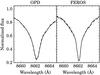 |
Fig. 1 OPD and FEROS subsamples with the two independently observed spectra of the same chromospherically inactive star over plotted. Left panel: the OPD spectra of HD 10700; right panel: the same for the FEROS spectra of HD 182572. The agreement between spectra observed in different runs is excellent for both spectrographs. |
H α sample.
Our data for the Hα sample were obtained in several observational runs between 1994 and 2008. As the NIR sample, the spectra were collected using coudé spectrograph of the 1.60 m OPD telescope. Over 14 yrs of observations, it was not possible to maintain the same instrumental setup, thus three different CCDs were used to collect our data: 2048×4608, 2048 ×2048 and 1024×1024 pixels with 13 μm, 13 μm and 24 μm of pixel size, respectively. We adopted a 1800 l/mm grating with 250 μm slit-width centered at 6563 Å yielding a nominal resolution of 45 000 for the 4608-pixel CCD and 20 000 for the remaining ones1. In order to maintain internal consistency, we adopted the same reduction procedures as discussed above for the NIR sample. The typical S/N of this sample is 180 and the distribution ranges from 40 to 420 wherein 90% of them have S/N> 100 (part of this sample was published in Lyra & Porto de Mello 2005).
We obtained spectroscopic Teffdeterminations for all stars of the Hα sample by fitting theoretical line profiles to the observed ones, following exactly the same prescriptions of Lyra & Porto de Mello (2005). Full details are given by these authors and here we merely summarize the essential aspects. The damping wings of the Hα line are classical Teffindicators (Gehren 1981; Barklem et al. 2002; Lyra & Porto de Mello 2005) for solar-type stars, being strongly Teffsensitive but showing little sensitivity to surface gravity, metallicity, microturbulent velocity, and NLTE effects. On the other hand, due to the breadth of the line wings, continuum placement is a significant source of error in the Teffdetermination. The use of echelle spectra thus hampers proper use of the method since a precise continuum normalization around Hα demands a consistent blaze correction over adjacent orders (Ramírez et al. 2014; Barklem et al. 2002), which is at best very difficult and often impossible. We therefore took advantage of our OPD single order spectra to obtain a precise and homogeneous normalization around the Hα profile and hence internally very consistent Teffs. The stellar metallicities were taken from assorted sources in the literature. To further enhance the internal consistency of the stellar atmospheric parameters we applied an empirical zero-point correction to the literature metallicites, adopting the HαTeff scale as homogeneous and correcting the [Fe/H] values by Δ[Fe/H] /ΔTeff = −0.06 dex/100 K, where ΔTeffis the difference between the literature Teffand the HαTeffobtained here.
As an additional consistent Teffdetermination, photometric Teffs were derived for all stars in the Hα benchmark sample from the calibrations of Porto de Mello et al. (2014), taking into account explicitly the corrected [Fe/H] values. The (B−V), (BT−VT), and (b−y) color indices were used, taken from the Hipparcos and the Olsen catalogues (Olsen 1983, 1993, 1994): all (b−y) photometry was converted to the Olsen (1993) scale according to prescriptions given by this author. The straight average between the Hα and the photometric Teffdeterminations was adopted as the Teffscale for the present work.
From Hipparcos parallaxes (van Leeuwen 2007), and the Teff, and [Fe/H] values derived above, we calculated stellar luminosities using bolometric corrections from Flower (1996). Masses and surface gravities were obtained from theoretical evolutionary tracks due to Kim et al. (2002) and Yi et al. (2003). We adopt this homogeneous scale of evolutionary surface gravities as our logg scale. Since it has recently become clear that the structural and temporal evolution of chromospheric activity is modulated by other parameters besides stellar age (Rocha-Pinto & Maciel 1998; Lyra & Porto de Mello 2005; Mamajek & Hillenbrand 2008), we purposefully buit a sample of field dwarfs and subgiants covering an extensive range of metallicities (from ≈−0.8 to +0.4 dex), and masses (from ≈0.7 to 1.5 M⊙). The atmospheric parameters Teff, [Fe/H] derived by us are given in Table 1 for the full Hα benchmark sample, also containing all of the stars considered for the construction of the Ca II IRT lines chromospheric indicator. The internal typical uncertainties for Teff(mean of Hα and photometric Teffs), [Fe/H] (from the literature but corrected for the homogeneous HαTeffscale), and log g(evolutionary) are, respectively, 50 K, 0.07 dex, and 0.1 dex. In Fig. 2 we show the distribution of stellar parameters derived in this work.
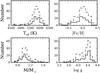 |
Fig. 2 Distributions of Teff, [Fe/H], mass, and log gof Hα and NIR samples represented by dashed and solid lines, respectively. |
Atmospheric parameters collected from the literature and derived in this work.
3. Absolute flux calibration
3.1. Total line flux equation
An important procedure in our analysis is the calculation of the emergent flux from the observed star whose relative scale is normalized by a pseudo-continuum in all spectra. Therefore, we do not have direct observational access to absolute purely radiative losses arising from stellar chromospheres. We then relate the observed f and intrinsic flux ℱ of a given star and integration bandwidth (Δλ) by the well-known relation: 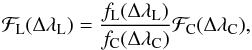 (1)where:
 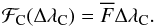 (2)Equation (1) is extremely important for our purposes because it relates directly to the absolute flux at the center of a specific spectral line ℱL through an empirical scaling factor given by the ratio of observed fluxes (
 ) which is multiplied by the absolute flux at the stellar continuum (ℱC(ΔλC)) in each reference region. Thus, we avoid the theoretical difficulties that arise from modeling the complex NLTE effects which are present at the center of intense spectral lines such as the Ca II IRT lines (Andretta et al. 2005) leaving only the absolute flux in the stellar continuum to be theoretically estimated by LTE models. The scale factor is observationally chosen in the observed spectra and is a function of the spectral resolution. Numerical integration is straightforwardly performed for the line and the continuum bands.
3.2. NMARCS atmospheric models
We calculated the theoretical continuum absolute fluxes using 1D, hydrostatic, plane-parallel LTE NMARCS spectra (Gustafsson et al. 2008) with a constant resolving power (R = λ/ Δλ = 20 000, 900 Å to 20 000 Å) along all the range covered by our observations, a value consistent with the resolution of our observed spectra (8340 Å to 8750 Å, R = λ/ Δλ ≈ 18 000 for the OPD data).
Based on the solar spectrum catalog of Utrecht (Moore et al. 1966) and also the Solar Flux Atlas of Kurucz et al. (1984), we identified a total of 5 continuum reference regions listed in Table 2. The identification of each RR is considerably straightforward since the density of photospheric transitions is quite low compared to shorter wavelengths. As an example, we show in Fig. 3 the theoretical spectrum of a solar-type star (Teff= 5500 K, log g= 4.4, and [Fe/H] = 0.0 dex), identifying the central wavelength of the reference regions by solid vertical lines.
Selected RR for the total absolute flux calculation.
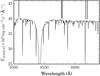 |
Fig. 3 Theoretical flux distribution model for a star cooler than the Sun (Teff= 5500 K, [Fe/H] = 0.0 e log g= 4.4 dex). The vertical lines indicate the central wavelength of the adopted reference regions. The large transition seen is the T2 line at λ8542. |
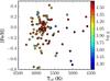 |
Fig. 4 Distribution of Teff, [Fe/H] for the sample stars, with the log gcolor coded. The atmospheric parameters of the entire sample is bracketed by the our NMARCS model atmosphere grid. |
The theoretical atmospheric model parameters range in Tefffrom 4500 K to 6500 K in steps of 250 K; the surface gravities (cgs units) from 3.0 to 5.0 dex in steps of 0.5 dex; and [Fe/H] from −1.0 to 0.5 dex in steps of 0.25 dex. For each reference region, we interpolate the fluxes  for specific values of Teff, log g, and [Fe/H]. The models completely cover the parameter space of our sample.
3.3. Absolute continuum flux calibration:
We next derive a calibration enabling the calculation of the model stellar absolute continuum flux () for each reference region as a function of the observational atmospheric parameters Teff, log g, and [Fe/H]. Various consistency tests with regressive models indicated that a cubic model shows neither departures from a normal distribution nor correlation between residuals and the model fluxes. The functional form adopted was the third-order polynomial given by: 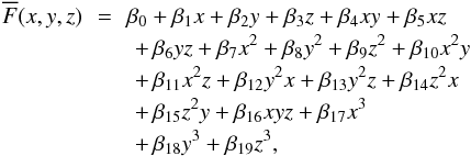 (3)where x = Teff/5777, y = log g, z = [Fe/H], and
  is in ×105 erg cm-2 s-1 Å-1 units.
We adopted an advanced variable selection procedure (Stepwise regression). A detailed discussion on this procedure is given by Ghezzi et al. (2014), and here we provide only the essencial aspects. For each reference region, we initialy fit a third-order polynomial and test iteratively the statistical significance of each term according to its hierarchy, starting from the highest order term. We then remove only the terms which decrease the previous fitting error (σFIT) and the BIC index (Bayesian Information Criteria, Kass & Raftery 1995). The iteractions continue until there are no possible removals leading to a final reduced model with the same predictive power of the complete ones. We provide, in Table 3, all the relevant information about the regressive model of absolute flux of each reference region. We see that in all RR that had removed variables, the ΔBIC lies between 4.7 and 15.9 indicating that the reduced models are more suitable than the complete ones (Kass & Raftery 1995). In Fig. 5, we show the distribution of the residuals for RR1. The typical standard deviation found is 0.05 × 10⁵ erg cm-2 s-1 Å-1.
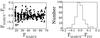 |
Fig. 5 Distribution (left panel) and histogram (right panel) of RR1 residuals for the cubic fitting model. Left panel: the differences between the NMARCS theoretical fluxes and the fluxes obtained from our regression models as a function of the NMARCS theoretical fluxes. Right panel: the distribution of the residuals from the relation showed in the left panel. The absolute continuum flux is in 105 erg cm-2 s-1 Å-1 units. |
Coefficients of the reduced regressive models.
We found Teffto be the major responsible for the variance of theoretical absolute continuum flux (≈90%), as expected, therefore transfering to all terms that include it a large statistical significance. The other variables (log gand [Fe/H]) combined account for ≈10%. For instance, we calculated the total continuum absolute fluxes for each RR, obtaining ≈4 × 10⁶ erg cm-2 s-1 which represents 3 orders of magnitude larger than σFIT (see Table 3). We expect the chromospheric component of a very inactive Sun-like star to be ≈105 erg cm-2 s-1 (see, for example, Figs. 11 and 12), 1−2 orders of magnitude higher than our fitting uncertainties. So, the absolute continuum calibration should not represent any significant additional source of error in the age-activity relations.
 |
Fig. 6 Impact of observational errors in the predicted absolute flux values of theoretical atmospheric models for the solar atmospheric parameters. We generate a distribution of absolute continuum flux based on 104 MC simulations assuming Gaussian uncertainties of 50 K, 0.1 dex, and 0.07 dex for Teff, log g, and [Fe/H], respectivelly. The typical standard deviation found in this distribution is ≈1.3 × 10⁵ erg cm-2 s-1. |
In Fig. 6, we show the impact of observational errors in the absolute continuum flux distribution,  (Teff, log g, [Fe/H]). We generated 104 Monte Carlo simulations for assuming a Gaussian distribution of the observational uncertainties of atmospheric parameters (σTeff = 50 K, σlog g = 0.1 dex, σ[Fe/H] = 0.07 dex). We calculated the standard deviation (σparameters) of the total flux distribution shown in Fig. 6 for RR1 and found typical values of 1.3 × 10⁵ erg cm-2 s-1 Å-1 (≈30% of solar chromospheric fluxes). When we propagate only Tefferrors in absolute fluxes, the flux variance turns out to be 1.2 × 10⁵ erg cm-2 s-1 Å-1, which corresponds to approximately 95% of σparameters, showing the great importance of the accurate determination of this parameter. However it must be emphasized that these errors are strongly correlated with Teff, which means that higher Teffleads to higher total line fluxes independent of the intrinsic chromospheric activity level. We expect to mitigate this residual correlation isolating the chromospheric component by a proper photospheric correction procedure. We will discuss the details of this procedure in Sects. 5 and 6.
3.4. Comparison with the literature: [Fe/H] bias
Hall (1996, hereafter H96) calibrated absolute continuum flux estimates ( ) for luminosity classes I−V covering the near ultraviolet (Ca II H & K) up to near infrared (Ca II IR triplet) region as a function of different color indices. To compare this with our results, we focus in his NIR calibration which is the region around T1 and T2 lines (λ8520). Depending on the color indices adopted, the errors derived from his functional relation were ≈10% which corresponds to ≈5 × 10⁵ erg cm-2 s-1 Å-1 in the solar case (Teff= 5777 K and [Fe/H] = 0.0). At this magnitude, the fitting errors will be of the same order of the chromospheric radiative losses of a typical inactive sun-like star.
In Fig. 7, we show the comparison between our RR1 fluxes calculated for the 250 stars with HαTeffin our benchmark sample and the λ8520 fluxes based on the (B−V) color index calibration taken from H96. Visually, the excellent agreement between the absolute continuum flux scales could be confirmed by a very strong linear correlation ρ = +0.93 (Spearman’s correlation). The [Fe/H] effects appear to be the most important that distinguish one relation from the other since a clear and systematic linear pattern could be detected as we analyzed the differences between the two determinations as a function of [Fe/H] (lower panel). For a given Teff, metal-rich stars have more efficient blocking of continuum radiation and, consequently, the temperature gradient of its deeper layers will be enhanced leading to an extra heating and flux (e.g. Edvardsson et al. 1993).
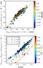 |
Fig. 7 Upper panel: comparison between Hall (1996) and our calibration of near-IR continuum absolute fluxes. Lower panel: strong [Fe/H] correlation in the differences between the absolute continuum flux estimates. The colors are related to different [Fe/H] (upper panel) and (B−V) (lower panel) estimates for each star. The solid lines are correction functions for specific (B−V) indices. |
We stress two points: 1) In the lower panel, the standard deviation of the differences between continuum fluxes is ≈3 × 10⁵ erg cm-2 s-1 Å-1 which is close to the fitting errors derived by H96 considering color indices; 2) Considering the typical levels of chromospheric radiative losses for stars after the Vaughan Preston Gap (≥2 Gyr), the [Fe/H] effects must have growing importance as we consider stars progressively more inactive. This result reinforces the need for a new absolute continuum calibration that has flexibility to distinguish the [Fe/H], Teff, and log gcontinuum effects. Probably, for stars with (B−V) ≤ 0.75, just a simple correction depending on [Fe/H] is enough to bring the Hall (1996) near-IR continuum fluxes to values closer to ours. However, for cooler stars, the [Fe/H] effect seems to be correlated with (B−V) as well, demanding a slightly more complex correction κ([Fe/H] , (B−V)): ![Mathematical equation: \begin{equation} \overline{F}_{RR1} = \overline{F}_{H96} + \kappa(\mathrm{[Fe/H]},{(B-V)}), \end{equation}](/articles/aa/full_html/2016/11/aa28825-16/aa28825-16-eq120.png) (4)where:
(4)where: ![Mathematical equation: \begin{eqnarray} \kappa(\mathrm{[Fe/H]},{(B-V)}) \!\!&=&\!\! - 4.94 + 9.36\mathrm{[Fe/H]} + 31.16{(B-V)} \nonumber \\ && + \, 2.13\mathrm{[Fe/H]}{({\it B-V})} + 1.44\mathrm{[Fe/H]}^2 \nonumber \\ && -\, 28.06{(B-V)}^2 \end{eqnarray}](/articles/aa/full_html/2016/11/aa28825-16/aa28825-16-eq121.png) (5)and the internal uncertainty of the flux conversion is σ = 0.29 × 10⁵ erg cm-2 s-1 Å-1.
(5)and the internal uncertainty of the flux conversion is σ = 0.29 × 10⁵ erg cm-2 s-1 Å-1.
4. Absolute total line fluxes: ℱL(ΔλL)
Returning to Eq. (1), we calculated the term  by numerical integrations leaving the integration bandwidth ΔλL around the Ca II IRT line cores a free parameter to be determined.
In Fig. 8 we show the normalized and ratio spectra of chromospherically active and inactive stars. These were chosen to possess similar atmospheric parameters in order to isolate the chromospheric activity differences. We identify two distinct regimes connected by a smooth transition. The first and more obvious one shows a sharp flux ratio contrast, suggesting that at lower optical depths (higher altitudes) there is an additional physical mechanism (chromospheric) to the second regime (photospheric) represented by an approximately constant flux ratio.
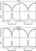 |
Fig. 8 Two selected ratio spectra from the FEROS and OPD samples. We choose pairs composed of an active (HD 28992 for the OPD and HD 165185 for FEROS samples) and an inactive star (HD 2151 for both samples). The profile differences in the line cores are mostly due to the chomospheric activity component. |
Given the problems linked to the arbitrariness on determining the exact interval around the center of Ca II IRT lines where the chromospheric component is predominant without too much influence of thermal processes, we chose pairs of similar stars composed of an active and inactive star and calculated their total absolute fluxes. In the absence of any a priori suitable initial value of the width of the interval of integration, we covered all possible values of ΔλL over an extensive domain ranging from bandwidths which evidently have a high contrast in total absolute flux rate (0.8 Å) to the upper limit (4.0 Å) where the width is clearly dominated by the photospheric component. In successive numerical integration, we adopt steps of 0.05 Å in order to ensure a continuous visual behavior, which facilitates interpretation regarding the variation of the total absolute fluxes ratio (ℛ) as function of the integration bandwidth (ΔλL). From these calculations, for each pair of stars, we calculated the first order gradient (∇ℛ) and second order (∇2ℛ) of this ratio represented mathematically by the set of equations  (6)
(6) (7)The average flux is given by the five adopted reference regions (Ri chosen for a particular band integration (
 ) around the center of each Ca II IRT line. The results are shown in Fig. 9.
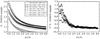 |
Fig. 9 Variation of the chromospheric flux component as a function of the integration bandwidth. Left: relation between the ℛ and the integration bandwidth around T3 spectral line (FEROS database). Right: the second order gradient of ℛ for the FEROS T3 line. There is a transition which connects two different regimes around Δλ = 2.0 Å. |
The dilution of the chromospheric component offers a basis for choosing the bandwidth for maximizing observationally the visibility of the chromospheric component. Additionally, the flux ratio differences between the pairs of stars are gradually removed as we consider the second derivative, converging to a single regime. For Δλ> 2.0 Å all pairs show the same dilution of the chromospheric component, in excellent agreement with a visual estimate of the visual spectra of Linsky et al. (1979a).
We applied the same procedure to the OPD subsample. Apparently instrumental effects make it more difficult to identify a smooth variation of ℛ with the increased integration bandwidth. Even so, it was possible to identify the need for a wider range of ΔλL in the OPD spectra defined as 2.2 Å. From these values, we calculate the total absolute flux on each Ca II IRT line based on Eq. (1).
To convert the subsamples to the same scale, we selected stars in common and fitted a linear function relating both subsamples2: 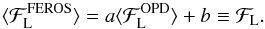 (8)Our choice of the integration bandwidths (
 Å and
Å and  Å) leads to conversion errors of σconv. ≈ 0.5 × 10⁵ erg cm-2 s-1, which represents typically 1% of ℱL. In Fig. 10, we show the adopted fit for the final subsample conversion of the T1 line and, in Table 4, we list the values of the regression coefficients calculated in the absolute total flux regression for the Ca II IRT lines T1 and T3.
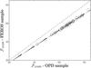 |
Fig. 10 Adopted fits for the conversion of T1 total absolute fluxes from OPD to the FEROS database. Black dots are observations in common; dashed line is the 1:1 relation, full line is the fit. |
Coefficents of the OPD-FEROS total absolute flux conversion.
Although some of our sample stars were observed over six years, it was not possible to quantify the influence of modulation of magnetic activity cycles. Therefore, any detected variability is interpreted as a result of uncertainties propagated by data reduction procedures as well as instrumental differences between each observational run. Such differences affect the accuracy of the total absolute flux scales calculated in observed spectra. Thus, we assume it to be a random effect that could be estimated by repeatability. We calculated the total absolute fluxes of the multiply observed stars and found low typical variations of ≈0.1−0.2 × 10⁵ erg cm-2s-1 (σrep) that, coupled with the uncertainties derived from the regressions (σreg and σparameters), provide total line flux errors (σTotal) of ≈1.3 to 1.4 × 10⁵ erg cm-2 s-1. The errors are given in Table 5. Observed absolute line fluxes are thus seem to be very stable and we can confidently treat our sample as fully homogeneous.
Derived errors in the absolute flux values.
5. Photospheric correction
We assume that the chosen integration interval for the measurement of total flux covers completely the chromospheric contribution, but also includes some photospheric contamination that must be properly removed. The major difficulty in measuring the chromospheric flux in photospheric strong lines lies in the fact that, in most cases, the desired quantity is one or two magnitudes smaller than the total and purely photospheric flux. As emphasized in a number of papers (Hartmann et al. 1984; Rutten & Schrijver 1987; Pasquini & Pallavicini 1991; Lyra & Porto de Mello 2005), the lack of knowledge regarding the photospheric flux distribution unfortunately imposes the adoption of arbitrary methods of correction. We now briefly discuss some techniques employed to carry out this task.
The works of Middelkoop (1982), Rutten (1984), and Noyes et al. (1984) enable the derivation of a normalized index of chromospheric activity independent of stellar spectral type, in principle, the  .
.
Despite the consistent results of chromospheric activity in open clusters, the strong correlation with X-rays, and rotational periods (Mamajek & Hillenbrand 2008), such non-dimensional indices may have complicated the physical interpretation, especially in the very low-activity regime (Hall et al. 2009). Furthermore, as we consider stars with a wide range of Teff, the normalization factor may contribute adding an explicit dependence on Teff(color), independent of intrinsic chromospheric fluxes (Rutten & Schrijver 1987).
Linsky et al. (1979a), inspired by Wilson (1968), compared stars with different levels of chromospheric activity and derived a function that represented the minimum chromospheric radiative losses given a color index (V−I). The difficulty of this method is to determine precisely which stars are adequate to establish a minimum level of magnetic activity as a function of Teff, or a proxy of it. Thus, it is imperative to populate the sample with a significant number of evolved stars for which we do expect systematically lower chromospheric radiative losses due to their angular momentum loss history.
It is noteworthy that this process is facilitated in samples like ours as we have the proper characterization of key parameters such as Teffand intrinsic luminosity. On the other hand, it is clear that this method is arbitrary and strongly dependent on the sample of stars being used. It establishes a null value of chromospheric radiative loss for stars that have a minimum level of activity for a specific Teff. In principle, this quantity does not vanish since we expect that some residual chromospheric basal heating in evolved stars should persist (Schrijver 1987).
We expect a strong correlation between ℱL and parameters closely related to the stellar structure. Thus, in Fig. 11, we confirm the Teffcorrelation and identify a second component that is minimally correlated to Teff, interpreted as the chromospheric flux. In order to remove the photospheric component, we assume a lower boundary of minimum magnetic activity given by the more inactive subgiants of our sample. Lyra & Porto de Mello (2005) found the same behavior for Hα line: the boundary is populated systematically by subgiants, as expected from stellar rotational evolution for this class of stars (do Nascimento et al. 2003). From this lower boundary, which is dependent on Teff, we subtract the thermal component by the relation:  (9)
(9)
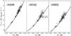 |
Fig. 11 Relations between the total absolute fluxes and Teffare shown for dwarfs (open squares) and subgiants (gray circles). The solid black lines are the lower boundary of minimum chromospheric activity represented by the more inactive subgiants. The 1.5 M⊙ subgiants HD 36553 and HD 112164 are the only stars placed bellow the photospheric correction curve. The panels are divided for the three Ca II IRT lines. Left and middle panels stand for the T1 and T2 lines, and the right one ilustrates the behavior of the T3 line. |
We emphasize that our procedure is rooted in the assumption that, to first order, the influence of photospheric flux is expressed mathematically in a separable way and dependent on a single parameter, the Teff. In Fig. 11 we show the ℱ vs. Teffdiagram for the Ca II triplet lines. We tested different orders of the polynomial photospheric subtraction functions from linear to cubic. As a result, due to a better agreement with the overall visual trend of ℱL and simpler form, we chose a third-order polynomial. Thus, the photospheric correction was performed for each star in our sample following:  (10)where X≡Teff/5777. In Table 6, we list the coefficients of Eq. (10) calculated for the Ca II IRT lines.
Coefficients of the third-order polynomial involved in the subtraction of the photospheric fluxes.
Two of the most massive subgiants in our sample, HD 36553 and HD 112124 (Teff≈ 5950 K, M ≈ 1.5 M⊙, log g≈ 3.7 dex and [Fe/H] ≈ +0.25 dex), are very similar and consistently placed below the minimum activity boundary for all Ca II IRT lines. These stars are at the tail of our sample distribution of masses, surface gravities, and metalicities (see Fig. 4). So, considering that these subgiants are not representative of our sample and to avoid the chromospheric flux superestimation of our hottest stars, we chose to remove them from the minimum activity boundary. This case is yet another reminder of the arbitrariness of such procedure and the strong bias that can be introduced by smaller and/or inadequately populated samples.
The photospheric subtraction procedure is well-constrained between 5100 K and 6100 K. Outside this domain, higher chromospheric flux uncertainties are expected since our fit deviates from the overall visual trend.
5.1. Algorithm to derive absolute chromospheric fluxes
We describe the necessary steps to derive the Ca II IRT chromospheric fluxes:
-
1.
Around each Ca II IRT line, calculate the observed line fluxfL (Sect. 4).
-
2.
For each reference region defined by Table 2, obtain the observed pseudo-continumm flux fC (Sect. 4). Then, with the help of Eqs. (2), (3), and Table 3, calculate the theoretical continuum absolute flux ℱC (which is defined as
 ) for a given set of atmospheric parameters. As a result, derive the absolute total line flux ℱL through Eq. (1).
 -
3.
Average all reference region estimates of ℱL obtaining ⟨ ℱL ⟩. Set ℱL≡⟨ ℱL ⟩.
-
4.
Calculate
 after correcting the photospheric signature of ℱL using Eq. (10) and Table 6 (Sect. 5).
 -
5.
The errors of these procedures are summarized in Table 5.
6. Uncertainty of chromospheric flux
In order to gauge the impact of atmospheric parameters uncertainties on the chromospheric flux scale, first, we chose a representative star of our sample, the solar-twin 18 Sco (Teff= 5809 K, [Fe/H] = +0.04 dex, and log g= 4.44 dex, Porto de Mello et al. 2014). We generated 104 MC simulations for its Teff, log g, and [Fe/H] assuming Gaussian uncertainties of 50 K, 0.1 dex, and 0.07 dex, respectivelly. The generated distribution of these parameters is shown in Fig. 12 (upper panels). Then, using the OPD spectra and the T2 line, for each MC simulation, we followed each steps described in Sect. 5.1 and derived the output distributions of total flux ℱλ8542 (middle left panel) and photospherically corrected flux (lower panel)  .
.
In the middle and lower panels of Fig. 12, a sharp profile indicates a residual correlation between the related quantities. The ℱλ8542 distribution is clearly above the minimum level of activity given by the photospheric correction (solid gray line) and strongly correlated with Teff, which accounts for the majority of total flux variance. After subtracting the 18 Sco photospheric component, we estimated the internal chromospheric flux errors ( ) of 0.3 × 10⁵ erg cm-2 s-1 which represent ≈8% of .
The impact of increasing uncertainties on Teffis considerably diminished by the behavior of the minimum activity boundary. For instance, 150 K errors around the 18 Sco’s Teff(which is 3σTeff) increase the chromospheric flux errors by ≤7%. Between 5400−6200 K, a simple scale shift of ±400 K in Teffmodifies the chromospheric flux scales slightly by an amount of ≤10% that is, certainly, compatible with . This result shows the consistency of our photospheric correction inside this domain. On the other hand, [Fe/H], which accounts for ≈10% of total flux variance (see Sect. 4), after the photospheric subtraction turns out to be the major source of . In the case of higher [Fe/H] errors of 0.21 dex (3σ[Fe/H]), increases by an amount of 300%. Therefore, this enforces the need of an accurate determination of [Fe/H] to avoid undesirable biases in the chromospheric activity distributions. Surface gravity effects are negligible (<3%)3.
The role of [Fe/H] and log guncertainties in active stars are expected to be minimized due to the strong contrast between the photospheric and chromospheric components. Nonetheless, these effects should be determining factors for inactive stars, especially those older than the Sun, if the age-activity relation is to be extended to the end of the main-sequence.
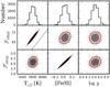 |
Fig. 12 18 Sco MC output distributions of ℱλ8542 and |
7. Conclusions
We derive absolute chromospheric fluxes in the Ca II IR triplet lines for 113 FGK stars, from high S/N and high-resolution spectra, covering an extensive range of atmospheric parameters and chromospheric activity levels. To this purpose, we derived the first near-IR continuum calibration anchored on NMARCS LTE models of atmospheres as an explicit function of Teff, [Fe/H], and log g. This procedure reduces the internal uncertainties in absolute continuum fluxes of Ca II IRT lines in order to enable a more consistent age-activity calibration of the solar-type stars. The internal errors on this analysis are two orders of magnitude smaller than in previous near-IR calibrations anchored in color indices. We also find excellent agreement between our absolute flux calibration and Hall (1996) corrected from [Fe/H] bias (σ = 0.29 × 10⁵ erg cm-2 s-1).
Through MC simulations, we find that the internal chromospheric flux error of each Ca II IRT line is 0.3 × 10⁵ erg cm-2 s-1 (≈10% of ). Owing to the proper photospheric correction, the activity distribution width does not depend primarily on the Teffuncertainties leaving [Fe/H] as the most important parameter in chromospheric flux variance. These new relations are especially important to bring into the same scale the chromospheric flux estimates of stars with different chemical composition, evolutionary states, and mass. Moreover, this approach provides a better understanding of the internal uncertainties and its dependencies with the atmospheric parameters. This new chromospheric flux calibration will be used in a forthcoming paper to investigate more comprehensively the age-activity relation of solar-type stars. Our reduced uncertainties enable us to explore the low-activity end of this relation, including older and less active stars. We also plan an extension of this method to late K and M dwarfs with precise ages (Garcés et al. 2011).
Since 2003, the Radial Velocity Experiment survey (RAVE) has been obtaining low-resolution spectra (R = 7500) in the near-infrared region (8410−8795 Å) for thousands of stars. In addition, the Gaia mission (Perryman et al. 2001) was successfully launched and will provide, in a unprecedented way, a 6-dimension map (positions and velocity components) for 109 stars in the Galaxy. In addition to the astrometric data, it will include a photometric and spectroscopic database of intermediate resolution (R = 7500−11 500) spectra in the Ca II IRT region for millions of late-type stars. Thus an adequate calibration of chromospheric fluxes along the lines we present could potentially allow age determinations for millions of stars.
For a few stars with V > 10 from Pleiades open cluster and HR 1614 SKG, the slit-width was changed to 500 μm yielding R = 10 000.
For T2, the conversion was not needed since it is not present in spectra of FEROS database.
The same behaviour of the T2 line as a function of atmospheric parameters was also found for the T1 and T3 lines.
Acknowledgments
We thank the anonymous referee for helpful comments. G.F.P.M. acknowledges financial support by the CNPq grant 476909/2006-6, the FAPERJ grant APQ1/26/170.687/2004, and the CAPES post-doctoral fellowship BEX 4261/07-0. D.L.S. acknowledges a scholarship from CNPq/PIBIC. D.L.S and L.D.F. acknowledge MSc CAPES scholarships. We thank the staff of the OPD/LNA for considerable support in the many observing runs carried out during this project. Use was made of the Simbad database, operated at the CDS, Strasbourg, France, and of NASA’s Astrophysics Data System Bibliographic Services. We thank Edward Guinan, José Dias do Nascimento Jr., and Jeffrey Hall for interesting discussions. I.R. acknowledges support from the Spanish Ministry of Economy and Competitiveness (MINECO) through grant ESP2014-57495-C2-2-R.
References
- Andretta, V., Busà, I., Gomez, M. T., & Terranegra, L. 2005, A&A, 430, 669 [NASA ADS] [CrossRef] [EDP Sciences] [Google Scholar]
- Baliunas, S. L., Donahue, R. A., Soon, W. H., et al. 1995, ApJ, 438, 269 [NASA ADS] [CrossRef] [Google Scholar]
- Barklem, P. S., Stempels, H. C., Allen de Prieto, C., et al. 2002, A&A, 385, 951 [NASA ADS] [CrossRef] [EDP Sciences] [Google Scholar]
- Busà, I., Aznar Cuadrado, R., Terranegra, L., Andretta, V., & Gomez, M. T. 2007, A&A, 466, 1089 [NASA ADS] [CrossRef] [EDP Sciences] [Google Scholar]
- Cauzzi, G., Reardon, K. P., Uitenbroek, H., et al. 2008, A&A, 480, 515 [NASA ADS] [CrossRef] [EDP Sciences] [Google Scholar]
- Chmielewski, Y. 2000, A&A, 353, 666 [NASA ADS] [Google Scholar]
- Dempsey, R. C., Bopp, B. W., Henry, G. W., & Hall, D. S. 1993, ApJS, 86, 293 [NASA ADS] [CrossRef] [Google Scholar]
- do Nascimento, Jr., J. D., Canto Martins, B. L., Melo, C. H. F., Porto de Mello, G., & De Medeiros, J. R. 2003, A&A, 405, 723 [NASA ADS] [CrossRef] [EDP Sciences] [Google Scholar]
- Edvardsson, B. 2008, Phys. Scr. T, 133, 014011 [NASA ADS] [CrossRef] [Google Scholar]
- Edvardsson, B., Andersen, J., Gustafsson, B., et al. 1993, A&A, 275, 101 [NASA ADS] [Google Scholar]
- Flower, P. J. 1996, ApJ, 469, 355 [NASA ADS] [CrossRef] [Google Scholar]
- Foing, B. H., Crivellari, L., Vladilo, G., Rebolo, R., & Beckman, J. E. 1989, A&AS, 80, 189 [NASA ADS] [Google Scholar]
- Garcés, A., Catalán, S., & Ribas, I. 2011, A&A, 531, A7 [NASA ADS] [CrossRef] [EDP Sciences] [Google Scholar]
- Gehren, T. 1981, A&A, 100, 97 [NASA ADS] [Google Scholar]
- Ghezzi, L., Dutra-Ferreira, L., Lorenzo-Oliveira, D., et al. 2014, AJ, 148, 105 [NASA ADS] [CrossRef] [Google Scholar]
- Gustafsson, B., Edvardsson, B., Eriksson, K., et al. 2008, A&A, 486, 951 [NASA ADS] [CrossRef] [EDP Sciences] [Google Scholar]
- Hall, J. C. 1996, PASP, 108, 313 [NASA ADS] [CrossRef] [Google Scholar]
- Hall, J. C., Lockwood, G. W., & Skiff, B. A. 2007, AJ, 133, 862 [NASA ADS] [CrossRef] [Google Scholar]
- Hall, J. C., Henry, G. W., Lockwood, G. W., Skiff, B. A., & Saar, S. H. 2009, AJ, 138, 312 [NASA ADS] [CrossRef] [Google Scholar]
- Hartmann, L., Soderblom, D. R., Noyes, R. W., Burnham, N., & Vaughan, A. H. 1984, ApJ, 276, 254 [NASA ADS] [CrossRef] [Google Scholar]
- Johnson, H. L. 1966, ARA&A, 4, 193 [NASA ADS] [CrossRef] [Google Scholar]
- Kass, R. E., & Raftery, A. E. 1995, J. Am. Stat. Assoc., 90, 773 [Google Scholar]
- Kim, Y.-C., Demarque, P., Yi, S. K., & Alexander, D. R. 2002, ApJS, 143, 499 [NASA ADS] [CrossRef] [Google Scholar]
- Krishnamurthi, A., Terndrup, D. M., Pinsonneault, M. H., et al. 1998, ApJ, 493, 914 [NASA ADS] [CrossRef] [Google Scholar]
- Kurucz, R. L., Furenlid, I., Brault, J., & Testerman, L. 1984, Solar flux atlas from 296 to 1300 nm (New Mexico: National Solar Observatory) [Google Scholar]
- Linsky, J. L., Hunten, D. M., Sowell, R., Glackin, D. L., & Kelch, W. L. 1979a, ApJS, 41, 481 [NASA ADS] [CrossRef] [Google Scholar]
- Linsky, J. L., McClintock, W., Robertson, R. M., & Worden, S. P. 1979b, ApJS, 41, 47 [NASA ADS] [CrossRef] [Google Scholar]
- Lovis, C., Dumusque, X., Santos, N. C., et al. 2011, ArXiv e-prints [arXiv:1107.5325] [Google Scholar]
- Lyra, W., & Porto de Mello, G. F. 2005, A&A, 431, 329 [NASA ADS] [CrossRef] [EDP Sciences] [Google Scholar]
- Mamajek, E. E., & Hillenbrand, L. A. 2008, ApJ, 687, 1264 [NASA ADS] [CrossRef] [Google Scholar]
- Middelkoop, F. 1982, A&A, 107, 31 [NASA ADS] [Google Scholar]
- Mihalas, D. 1978, Stellar atmospheres, 2nd edn. (San Francisco: W. H. Freeman and Co) [Google Scholar]
- Mittag, M., Schmitt, J. H. M. M., & Schröder, K.-P. 2013,A&A, 549, A117 [Google Scholar]
- Moore, C. E., Minnaert, M. G. J., & Houtgast, J. 1966, The Solar Spectrum 2935 Å to 8770 Å (Washington: Nat. Bur. Std. Monograph, USGPO) [Google Scholar]
- Noyes, R. W., Hartmann, L. W., Baliunas, S. L., Duncan, D. K., & Vaughan, A. H. 1984, ApJ, 279, 763 [NASA ADS] [CrossRef] [Google Scholar]
- Olsen, E. H. 1983, A&AS, 54, 55 [NASA ADS] [Google Scholar]
- Olsen, E. H. 1993, A&AS, 102, 89 [NASA ADS] [Google Scholar]
- Olsen, E. H. 1994, A&AS, 104, 429 [NASA ADS] [Google Scholar]
- Parker, E. N. 1970, ApJ, 162, 665 [NASA ADS] [CrossRef] [Google Scholar]
- Pasquini, L., & Pallavicini, R. 1991, A&A, 251, 199 [NASA ADS] [Google Scholar]
- Perryman, M. A. C., de Boer, K. S., Gilmore, G., et al. 2001, A&A, 369, 339 [NASA ADS] [CrossRef] [EDP Sciences] [Google Scholar]
- Porto de Mello, G. F., da Silva, R., da Silva, L., & de Nader, R. V. 2014, A&A, 563, A52 [NASA ADS] [CrossRef] [EDP Sciences] [Google Scholar]
- Ramírez, I., Fish, J. R., Lambert, D. L., & Allen de Prieto, C. 2012, ApJ, 756, 46 [NASA ADS] [CrossRef] [Google Scholar]
- Ramírez, I., Allende Prieto, C., & Lambert, D. L. 2013, ApJ, 764, 78 [NASA ADS] [CrossRef] [Google Scholar]
- Ramírez, I., Meléndez, J., Bean, J., et al. 2014, A&A, 572, A48 [NASA ADS] [CrossRef] [EDP Sciences] [Google Scholar]
- Rocha-Pinto, H. J., & Maciel, W. J. 1998, MNRAS, 298, 332 [NASA ADS] [CrossRef] [Google Scholar]
- Rutten, R. G. M. 1984, A&A, 130, 353 [NASA ADS] [Google Scholar]
- Rutten, R. G. M., & Schrijver, C. J. 1987, A&A, 177, 155 [NASA ADS] [Google Scholar]
- Santos, N. C., Israelian, G., & Mayor, M. 2004, A&A, 415, 1153 [NASA ADS] [CrossRef] [EDP Sciences] [Google Scholar]
- Schrijver, C. J. 1987, A&A, 172, 111 [NASA ADS] [Google Scholar]
- Skumanich, A. 1972, ApJ, 171, 565 [NASA ADS] [CrossRef] [Google Scholar]
- Terrien, R. C., Mahadevan, S., Bender, C. F., Deshpande, R., & Robertson, P. 2015, ApJ, 802, L10 [NASA ADS] [CrossRef] [Google Scholar]
- van Leeuwen, F. 2007, A&A, 474, 653 [NASA ADS] [CrossRef] [EDP Sciences] [Google Scholar]
- Wilson, O. C. 1968, ApJ, 153, 221 [NASA ADS] [CrossRef] [Google Scholar]
- Yi, S. K., Kim, Y.-C., & Demarque, P. 2003, ApJS, 144, 259 [NASA ADS] [CrossRef] [Google Scholar]
- Žerjal, M., Zwitter, T., Matijevič, G., et al. 2013, ApJ, 776, 127 [NASA ADS] [CrossRef] [Google Scholar]
All Tables
Coefficients of the third-order polynomial involved in the subtraction of the photospheric fluxes.
All Figures
|
Fig. 1 OPD and FEROS subsamples with the two independently observed spectra of the same chromospherically inactive star over plotted. Left panel: the OPD spectra of HD 10700; right panel: the same for the FEROS spectra of HD 182572. The agreement between spectra observed in different runs is excellent for both spectrographs. |
| In the text | |
|
Fig. 2 Distributions of Teff, [Fe/H], mass, and log gof Hα and NIR samples represented by dashed and solid lines, respectively. |
| In the text | |
|
Fig. 3 Theoretical flux distribution model for a star cooler than the Sun (Teff= 5500 K, [Fe/H] = 0.0 e log g= 4.4 dex). The vertical lines indicate the central wavelength of the adopted reference regions. The large transition seen is the T2 line at λ8542. |
| In the text | |
|
Fig. 4 Distribution of Teff, [Fe/H] for the sample stars, with the log gcolor coded. The atmospheric parameters of the entire sample is bracketed by the our NMARCS model atmosphere grid. |
| In the text | |
|
Fig. 5 Distribution (left panel) and histogram (right panel) of RR1 residuals for the cubic fitting model. Left panel: the differences between the NMARCS theoretical fluxes and the fluxes obtained from our regression models as a function of the NMARCS theoretical fluxes. Right panel: the distribution of the residuals from the relation showed in the left panel. The absolute continuum flux is in 105 erg cm-2 s-1 Å-1 units. |
| In the text | |
|
Fig. 6 Impact of observational errors in the predicted absolute flux values of theoretical atmospheric models for the solar atmospheric parameters. We generate a distribution of absolute continuum flux based on 104 MC simulations assuming Gaussian uncertainties of 50 K, 0.1 dex, and 0.07 dex for Teff, log g, and [Fe/H], respectivelly. The typical standard deviation found in this distribution is ≈1.3 × 10⁵ erg cm-2 s-1. |
| In the text | |
|
Fig. 7 Upper panel: comparison between Hall (1996) and our calibration of near-IR continuum absolute fluxes. Lower panel: strong [Fe/H] correlation in the differences between the absolute continuum flux estimates. The colors are related to different [Fe/H] (upper panel) and (B−V) (lower panel) estimates for each star. The solid lines are correction functions for specific (B−V) indices. |
| In the text | |
|
Fig. 8 Two selected ratio spectra from the FEROS and OPD samples. We choose pairs composed of an active (HD 28992 for the OPD and HD 165185 for FEROS samples) and an inactive star (HD 2151 for both samples). The profile differences in the line cores are mostly due to the chomospheric activity component. |
| In the text | |
|
Fig. 9 Variation of the chromospheric flux component as a function of the integration bandwidth. Left: relation between the ℛ and the integration bandwidth around T3 spectral line (FEROS database). Right: the second order gradient of ℛ for the FEROS T3 line. There is a transition which connects two different regimes around Δλ = 2.0 Å. |
| In the text | |
|
Fig. 10 Adopted fits for the conversion of T1 total absolute fluxes from OPD to the FEROS database. Black dots are observations in common; dashed line is the 1:1 relation, full line is the fit. |
| In the text | |
|
Fig. 11 Relations between the total absolute fluxes and Teffare shown for dwarfs (open squares) and subgiants (gray circles). The solid black lines are the lower boundary of minimum chromospheric activity represented by the more inactive subgiants. The 1.5 M⊙ subgiants HD 36553 and HD 112164 are the only stars placed bellow the photospheric correction curve. The panels are divided for the three Ca II IRT lines. Left and middle panels stand for the T1 and T2 lines, and the right one ilustrates the behavior of the T3 line. |
| In the text | |
|
Fig. 12 18 Sco MC output distributions of ℱλ8542 and |
| In the text | |
Current usage metrics show cumulative count of Article Views (full-text article views including HTML views, PDF and ePub downloads, according to the available data) and Abstracts Views on Vision4Press platform.
Data correspond to usage on the plateform after 2015. The current usage metrics is available 48-96 hours after online publication and is updated daily on week days.
Initial download of the metrics may take a while.