| Issue |
A&A
Volume 691, November 2024
|
|
|---|---|---|
| Article Number | A304 | |
| Number of page(s) | 17 | |
| Section | Stellar atmospheres | |
| DOI | https://doi.org/10.1051/0004-6361/202452025 | |
| Published online | 21 November 2024 | |
Chromospheric Mg I emission lines of pre-main-sequence stars★
1
Institute of Space and Astronautical Science, Japan Aerospace Exploration Agency,
3-1-1 Yoshinodai, Chuo-ku, Sagamihara,
Kanagawa
252-5210,
Japan
2
Nishi-Harima Astronomical Observatory, Center for Astronomy, University of Hyogo,
407-2 Nishigaichi, Sayo, Sayo,
Hyogo
679-5313,
Japan
3
Subaru Telescope, National Astronomical Observatory of Japan,
650 North A’ohoku Place,
Hilo,
HI
96720,
USA
★★ Corresponding author; This email address is being protected from spambots. You need JavaScript enabled to view it.
Received:
28
August
2024
Accepted:
30
September
2024
Abstract
Context. To reveal details of the internal structure, the relationship between chromospheric activity and the Rossby number has been extensively examined for main-sequence stars. For active pre-main-sequence (PMS) stars, it is suggested that the level of activity be assessed using optically thin emission lines, such as Mg I.
Aims. We aim to detect Mg I chromospheric emission lines from PMS stars and to determine whether the chromosphere is activated by the dynamo process or by mass accretion from protoplanetary disks.
Methods. We analyzed high-resolution optical spectra of 64 PMS stars obtained with the Very Large Telescope (VLT)/X-shooter and UVES and examined the infrared Ca II (8542 Å) and Mg I (8807 Å) emission lines. To detect the weak chromospheric emission lines, we determined the atmospheric parameters (Teff and log 𝑔) and the degree of veiling of the PMS stars by comparing the observed spectra with photospheric model spectra.
Results. After subtracting the photospheric model spectrum from the PMS spectrum, we detected Ca II and Mg I as emission lines. The strengths of the Mg I emission lines in PMS stars with no veiling are comparable to those in zero-age main-sequence (ZAMS) stars if both types of stars have similar Rossby numbers. The Mg I emission lines in these PMS stars are thought to be formed by a dynamo process similar to that in ZAMS stars. In contrast, the Mg I emission lines in PMS stars with veiling are stronger than those in ZAMS stars. These objects are believed to have protoplanetary disks, where mass accretion generates shocks near the photosphere, heating the chromosphere.
Conclusions. The chromosphere of PMS stars is activated not only by the dynamo process but also by mass accretion.
Key words: accretion, accretion disks / techniques: spectroscopic / stars: chromospheres / stars: low-mass / stars: pre-main sequence / stars: rotation
Just to show the usage of the elements in the author field.
© The Authors 2024
 Open Access article, published by EDP Sciences, under the terms of the Creative Commons Attribution License (https://creativecommons.org/licenses/by/4.0), which permits unrestricted use, distribution, and reproduction in any medium, provided the original work is properly cited.
This article is published in open access under the Subscribe to Open model. This email address is being protected from spambots. You need JavaScript enabled to view it. to support open access publication.
1 Introduction
The atmosphere above the photosphere is called the chromosphere. The chromosphere is optically thin, with the optical depth gradually decreasing from τ5000 Å ≈ 10−4 to ≈10−7 as altitude increases (Frohlich & Lean 2004). In an active chromospheric region, atoms emit permitted lines such as Hα and Ca II. Chromospheric activity is thought to be driven by the magnetic field generated by the dynamo process.
For pre-main-sequence (PMS) stars, several researchers have suggested that chromospheric emission lines are also influenced by mass accretion. Hamann & Persson (1992) conducted optical spectroscopy of PMS stars and found that narrow emission lines, such as Ca II and Mg I (e.g., 8807 Å), are generated in the stellar chromosphere, while broad emission lines result from mass accretion. Mohanty et al. (2005) investigated the chromospheric activity of classical T Tauri stars (CTTSs), very low-mass young stars (0.075 ≤ M* < 0.15 M⊙), and young brown dwarfs (M* ≤ 0.075 M⊙). The surface flux of the Ca II emission line at 8662 Å, F′8662 correlate with the mass accretion rate, Ṁ, for approximately four orders of magnitude. This led them to conclude that the Ca II emission line is an excellent quantitative measure of the accretion rate. Batalha et al. (1996) found correlations with veiling and near-infrared excesses, attributing the Ca II and He I emission lines to a “hot chromosphere” heated by accretion shocks.
Yamashita et al. (2020) investigated the relationship between the Rossby number, NR (= defined as the rotational period, P, divided by the convective turnover time, τc), and R′8498, R′8542, and R′8662, which represent the ratio of the surface flux of the Ca II infrared triplet (IRT) emission lines (8498, 8542, 8662 Å) to the stellar bolometric luminosity, for 60 PMS stars. Only three PMS stars exhibit broad and strong emissions, indicative of significant mass accretion. Most PMS stars show narrow and weak emissions, suggesting that their emission lines are formed in the chromosphere. All their Ca II IRT emission lines have R′IRT ∼ 10−4.2, comparable to the maximum R′IRT observed in ZAMS stars. The PMS stars exhibit NR < 10−0.8 and a constant R′IRT with respect to NR, indicating that their Ca II IRT emission lines are saturated.
Yamashita & Itoh (2022) have demonstrated that Mg I emission lines are a good indicator of activity in fast-rotating and active ZAMS stars. They examined the infrared Mg I emission lines at 8807 Å for 47 ZAMS stars in IC 2391 and IC 2602 using archive data from the University College London Echelle Spectrograph on the Anglo-Australian Telescope. They found that ZAMS stars with smaller Rossby numbers exhibit stronger Mg I emission lines, even among stars in the Ca II saturated region.
In this study, we measure the strength of Mg I emission lines in 64 PMS stars and investigate whether their chromospheres are activated by the dynamo process or mass accretion. We compare the strength of the chromospheric emission lines in PMS stars with that in ZAMS stars from young open clusters. In the following section, we describe the high-resolution spectroscopic data and the reduction procedures. Sect. 3 presents the results, and Sect. 4 discusses the origin of the Mg I emission lines and their emitting regions on the stellar surface.
2 Datasets and data reduction
2.1 Datasets
Our targets include 64 G, K, and M-type PMS stars from four star-forming regions and seven moving groups: the Taurus- Auriga molecular cloud, the ρ Ophiuchi molecular cloud, the Lupus star-forming region, the Chamaeleon I star-forming region, the Orionis OB 1c association, the Upper Scorpius association, the AB Doradus moving group, the β Picoris moving group, the “Cha-Near” region, the η Chamaeleontis cluster, and the TW Hydrae association. Hereafter, objects from these starforming regions and moving groups are referred to as PMS stars. The metallicity of PMS stars in these regions and groups has been determined to be similar to that of the Sun. We did not include binaries or triplets listed in Ghez et al. (1993), Kraus et al. (2009), Kraus et al. (2012), Neuhauser et al. (1995), Leinert et al. (1993), Wahhaj et al. (2010), and Zuckerman & Song (2004). All of the targets investigated in this study are listed in Table A.1.
We used archival data of 59 PMS stars obtained with X-shooter (R ∼ 8, 000) mounted on the Very Large Telescope (VLT). The program IDs, observation dates, and integration times are listed in Table A.2. The wavelength coverage was from 2989 Å to 10 200 Å, with integration times ranging from 2 s to 4360 s. Additionally, we used archival data of five PMS stars obtained with Ultraviolet and Visual Echelle Spectrograph (UVES, R ∼ 40 000) mounted on the VLT. The wavelength coverage was from 3732 Å to 9496 Å, with integration times ranging from 10 s to 600 s.
2.2 Photometry
To obtain the rotational period, we analyzed the Pre-search Data Conditioning Simple Aperture Photometry (PDCSAP) fluxes observed with the Transiting Exoplanet Survey Satellite (TESS). The PDCSAP fluxes were derived by aperture photometry1. We calculated the average of PDCSAP fluxes for each star, and the standard deviation of the flux, σ1, then removed the flux data points greater than 3σ1 above the average. We then searched for periodicity in the signals by conducting Lomb–Scargle (Scargle 1982) periodogram analysis. For each object, the period of the light curve, P, was determined.
We believe that the main component of the period in the TESS light curve is due to stellar spots on their surface, not other sources such as occultation by a disk or mass accretion. First, the protoplanetary disk is flared with radial distance from the central stars (Hartmann et al. 2016). A central star would be hidden by the outer edge of the disk, if the inclination angle of the system were large. However, such edge-on disk objects, which are observed from the direction of the disks, are rare. Second, the variable light caused by the obscuration of the disk could be on the order of years. The outer edge (∼100 AU) of the Keplerian disk orbits in a hundred years. A variation of a hundred years is not detected during the TESS observation of 27 days. Third, mass accretion is predicted to be not stable, but highly time-variable, with much of the mass having been accreted in short bursts (Kenyon et al. 1990, 1994). Therefore, we considered the period of all PMS stars to be caused by the spots, not only the periodic group, but also quasiperiodic symmetric and burster groups. We note that those discussions are only adopted with regard to the variation period. The amplitude of the light curves should involve spot modulation, occultation by a disk, or mass accretion.
We also reject the possibility that the PMS stars show light variation caused by pulsation. Rebull et al. (2016) identified the A-type and early F-type stars with a period of ≤0.3 days as pulsators. In this study, only HIP 17695, a K0-type star, shows variable light with a period of ≤0.3 days. The measured period in this study is considered to be the rotation period caused by a spot on the surface of a PMS star.
2.3 Spectroscopy
We used the Image Reduction and Analysis Facility (IRAF) software package2 for data reduction. The X-shooter and UVES data had already been reduced up to the point before wavelength calibration. To improve the signal-to-noise ratio (S /N), we combined and averaged multiple frames taken on the same day for each object, applying weights proportional to the integration time of each frame. The target spectra were contaminated by Earth’s atmospheric absorption. We removed telluric absorption lines using the Advanced Cerro Paranal Sky Model provided by European Southern Observatory (Noll et al. 2012; Jones et al. 2013).
We subtracted the photospheric absorption components from all spectra using stellar photosphere spectral models. Generally, the photospheric absorption components of the Ca II IRT and Mg I lines are strong, particularly for K-type stars. The Mg I emission component is often obscured by the photospheric absorption, as is illustrated in Fig. 1.
2.3.1 Determination of the atmospheric parameters (Teff and log g), veiling value (r), and line broadening
To detect the weak chromospheric emission lines, we determined the atmospheric parameters (Teff and log g), the amount of veiling (r), and line broadening of the PMS stars in two steps. We compared the observed spectra with photospheric model spectra using the Phoenix-BT-Dusty models (Kulenthirarajah et al. 2019) from the POLLUX database (Palacios et al. 2010). Initially, we obtained 280 models with effective temperatures ranging from 2000 K to 6000 K (in 100 K steps), log g values from 2.0 to 5.0 dex (in 0.5 dex steps), and a solar iron abundance (Table 1). This grid encompasses the range of our targets and extends to lower gravities typical of giants.
For the correction of rotational broadening, we convolved the model spectra with a Gaussian kernel in 26 steps of σ, corresponding to v sin i values ranging from 0 to 250 km s−1. Convolution with a Gaussian function of large σ caused the continuum level of the model spectrum to decrease because broad absorption lines often blend with other strong lines. After convolving with the Gaussian kernel, we renormalized the continuum for all the model spectra.
An absorption line profile of a PMS spectrum might be obscured by continuum veiling. The amount of veiling, r, is defined as
 (1)
(1)
The equivalent width (EQW) of an absorption line in an unveiled spectrum is denoted by W0, and W represents the EQW of a line in a veiled spectrum. We set the veiling parameter, r, between 0 and 5 in 20 steps. First, we added the veiling value, r, to the normalized model spectrum. We then renormalized the continuum to unity by dividing by (1 + r).
We subtracted each model spectrum from the observed spectra of the 64 PMS stars and evaluated the fit quality. In the first step, we selected four regions for fitting the spectra, based on the work of Frasca et al. (2017): 6050–6270 Å (main features: CaI, Fe I, TiO), 7020–7120 Å (TiO), 7600–7720 Å (KI, Fe II), and 8160–8222 Å (Na I, VI). According to Frasca et al. (2017), these regions are particularly suitable for determining Teff, log g, v sin i, and veiling. It should be noted that the wavelength range of 5120–6270 Å is not available for some PMS stars observed with UVES. For each wavelength range, we measured the standard deviation of the count values of the residual spectrum, S (i). Fig. 1 illustrates the spectral subtraction procedure for the photospheric component in PMS stars. Many Fe I absorption lines are present in both the target and model spectra, as is shown in the hatched area of Fig. 1a. Emission components of Fe I may originate in the lower chromosphere (Vernazza et al. 1981). Highly active T Tauri stars exhibit narrow Fe I and Fe II emission lines at rest velocity, believed to be formed in the chromosphere (Hamann & Persson 1992), and ZAMS stars also show narrow Fe I emission lines (Yamashita & Itoh 2022). We excluded wavelengths near strong Fe I lines from the fitting range if their g f value exceeded 10−1.3. Here, we determined the σ value of the model with the smallest S (i) in each spectral region. Then, we determined Teff, log g, and r if the sum of squares of the standard deviation, S (i), was the smallest. Teff and log g are one value for one object, respectively, whereas different values of r were determined for the different spectral regions. Following Frasca et al. (2017), in the second step, we included one or two additional blue spectral regions for objects with temperatures higher than 3500 K. For UVES data, these regions are 4400–4580 Å (main features: Fe I), while for X-shooter data, we added 4400–4580 Å and 5120–5220 Å (Mg I triplet). We then recalculated the sum of the squares of S (i) and redetermined Teff, log g, r, and σ.
For each object, we estimated the errors in temperature and surface gravity. We defined Ti as the temperature of the model with the smallest S (i). The error in temperature was calculated as the standard deviation of Ti, given by  . The error in surface gravity was estimated using the same procedure.
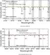 |
Fig. 1 Procedure for subtracting the photospheric component from PMS star spectra. The top portion of each panel shows the observed spectrum (solid line), while the model spectrum is represented by the dashed line. For display purposes, the spectra of the PMS stars and the models are shifted by +1.0 or +2.0. The bottom portion of each panel displays the difference between the PMS star spectrum and the model spectrum. Hatched areas indicate Fe I, Ca II, and Mg I lines. Wavelengths within these hatched areas have been excluded from the fitting range. |
Physical parameters of the model spectra.
2.3.2 Veiling measurements near the chromospheric emission lines and detection of the emission lines
Fig. 1b illustrates the procedure for spectral subtraction near the Ca II and Mg I lines for AA Tau. In this case, the Ca II line shows an emission profile superimposed on a broad absorption feature in the observed spectrum. We subtracted the model spectrum from the observed spectrum of the PMS star. The dashed line in Fig. 1b represents the best-fit model spectrum. We determined r in the following wavelength ranges: 8420–8560 Å for Ca II lines at 8498 and 8542 Å, 8560–8700 Å for the Ca II line at 8662 Å, and 8700–8850 Å for the Mg I line at 8807 Å. Wavelengths close to the strong emission lines, shown in the hatched area in Fig. 1b, were excluded from the fitting range.
Before measuring the EQWs, we normalized the spectra after subtracting the photospheric absorption components to unity. To obtain the EQWs of the Mg I and Ca II emission lines, we integrated the areas of the corresponding emission profiles directly. The EQW errors were estimated by multiplying the standard deviation of the continuum by the wavelength range of the emission lines for each PMS star. We derived the standard deviations of the continua near the emission lines using the following wavelength ranges: 8483–8492 Å for Ca II lines at 8498 and 8542 Å, 8623–8632 Å for Ca II at 8662 Å, and 8798–8802 Å and 8813– 8819 Å for the Mg I emission line. No strong features were observed within these wavelength ranges.
3 Results
3.1 Teff and log g, and veiling
The effective temperature (Teff), surface gravity (log g), and veiling value (r) for 64 PMS stars were determined (Table A.3). Typical uncertainties are ≈300 K for the effective temperature, and ≈0.8 dex for surface gravity. To assess the accuracy of Teff, we compared the Teff values for six Lupus objects determined in this study with those reported in Frasca et al. (2017). This comparison is shown in Fig. 2. The Teff values from both studies are comparable, with a correlation coefficient of 0.981. We conclude that the temperatures we derived for the other 64 PMS stars are accurate. LkCa 4 and LkCa 15 were observed on two separate occasions. The measured Teff and log g values did not differ between observations, although the chromospheric emission lines exhibited time variations. This indicates that atmospheric parameters can be accurately measured even for PMS stars with time-varying chromospheric emission lines.
Most of the PMS stars show veiling with r ≥ 0.1. In particular, for the highly veiled 28 PMS stars (r ≥ 0.6 at 4400 Å or 5120 Å), the amount of veiling increases as the wavelengths decrease. In previous studies, the high veiling with a peak in the ultraviolet region has been observed for strongly accreting PMS stars. This is considered to be due to the heated photosphere below the mass accretion shock. Basri & Batalha (1990) investigated the wavelength dependence of optical veiling for 16 T Tauri stars. For the five T Tauri stars out of 16 T Tauri stars, the amounts of veiling increase with decreasing wavelengths between 4000–5500 Å and are flat for λ ≥ 5500 Å. This is similar to the results achieved in this study.
Fig. 3 presents the HR diagram of the investigated PMS stars. The luminosity was estimated from the i-band magnitude with the corrections of the interstellar extinction and the amount of the veiling. The distance of the objects was mainly taken from Gaia Data Release 2 (Bailer-Jones et al. 2018). The distances of RY Tau and COUP 1287 were taken from Gaia Early Data Release 3 (Gaia Collaboration 2021), and that of RECX 09 was taken from Mamajec et al. (2000). We estimated the mass, age, and convective turnover time (τc) of the PMS stars by using the evolutionary models presented by Jung & Kim (2007), which is one of the few evolutionary tracks that takes into account the evolution of the internal structure of PMS stars to determine the convection turnover time. We linearly interpolated that model to one tenth of the original. The stellar age, mass, and τc are listed in Table A.4.
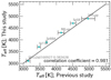 |
Fig. 2 Comparison between the effective temperature determined in this study and that derived from the spectroscopic study of Frasca et al. (2017). |
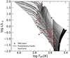 |
Fig. 3 HR diagram of the investigated PMS stars. The solid and dashed lines denote the evolutionary tracks (0.065–4.5 M⊙) and isochrones (2 × 10⁵ yr to the main sequence) of Jung & Kim (2007). We linearly interpolated that model to one tenth of the original. The thick solid line denotes the evolutionary track for a 1 M⊙ star. The circles represent the PMS stars. |
Examples of the chromospheric emission lines detected from 64 PMS stars.
3.2 Chromospheric emission lines
Mg I emission lines (8807 Å) were detected in 48 out of 64 PMS stars. Figs. A.1 and A.2 show the Mg I line (8807 Å) spectra of the PMS stars after subtracting the photospheric absorption. The EQWs and FWHMs of the chromospheric emission lines of Ca II IRT (8542 Å) and Mg I (8807 Å) are listed in Table A.5. The PMS stars show Ca II emission lines at 8542 Å, ranging from 0.07 Å to 43 Å. In Marsden et al. (2009), the EQWs of the ZAMS stars are between 0.10 Å and 94 Å. The EQWs of the stars in both studies are comparable. The PMS stars show Mg I emission lines whose EQWs range from 0.04 Å to 0.52 Å. In Yamashita & Itoh (2022), the EQWs of the Mg I emission lines range from 0.02 Å to 0.52 Å for the ZAMS stars. The EQWs of the PMS stars are comparable to those of the ZAMS stars.
As is noted by Yamashita & Itoh (2022), Mg I emission lines at 8807 Å were detected during a total solar eclipse (Dunn et al. 1968). Additionally, some chromospheric emission lines observed during a total solar eclipse (Dunn et al. 1968) are also detected in the PMS spectra after subtracting the absorption components in the 8650–8850 Å range, including Si I (8728 Å), P12(8750 Å), and Fe I (8680, 8824, 8838 Å). Among these, P12 and Fe I at 8824 Å were also observed in the T Tauri star spectra obtained by Hamann & Persson (1992), who performed optical spectroscopy of 34 PMS stars with high accretion rates. Table 2 provides examples of the chromospheric emission lines detected from 64 PMS stars in this study and the number of PMS stars with detected emission lines. Hamann & Persson (1992) did not subtract the photospheric absorption components but detected Mg I and Fe I (8807, 8824 Å) emission lines in eight T Tauri stars. Further, in this study, the minimum EQW of the Mg I emission lines is 0.04 Å, while that in Hamann & Persson (1992) was 0.37 Å. In this study, after subtracting the photospheric absorption components, we detected these emission lines in a larger number of PMS stars and weaker emission lines. We conclude that subtracting the model spectrum is essential for detecting weak emission lines.
4 Discussion
4.1 Veiling and infrared excess
Fig. 4 is the near-infrared color–color diagram for the PMS stars. We estimated the quantities of intrinsic near-infrared excess using the method described in Hosoya et al. (2019). The amount of near-infrared excess for the PMS stars was determined by the intersection of the reddening vector originating from the observed JHK colors and the intrinsic colors for CTTSs. The zero point of the intrinsic near-infrared excess is defined as the intersection of a line parallel to the reddening vector through an M6 dwarf color and the intrinsic CTTS line, (J − H, H − K) = (0.79, 0.47). The point of unity for near-infrared excess is defined as the reddest intrinsic color of CTTSs, (J − H, H −K) = (1.1, 1.0) (Meyer et al. 1997). Excess values are listed in Table A.1, ranging from −0.68 to 0.91. Of the PMS stars in this study, 37 show no excess (≤0), while 14 PMS stars show excess (>0). We did not calculate excess values for PMS stars below the line parallel to the reddening vector through an M6 dwarf color and the intrinsic CTTS line.
In Section 3.1, we reported that some highly veiled PMS stars exhibit a greater amount of veiling at shorter wavelengths, which is thought to be due to the heated photosphere below the shock resulting from mass accretion from a protoplanetary disk. The color-color diagram is a valuable tool for examining the presence of protoplanetary disks. However, one-third of CTTSs do not show significant infrared excess (Meyer et al. 1997). Spectroscopy allows us to detect veiling caused by the heated photosphere, indicating mass accretion from a protoplanetary disk. Indeed, the six PMS stars without excess in Fig. 4 show veiling amounts of 0.1–0.2 in the 8798–8802 and 8813–8819 Å regions.
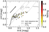 |
Fig. 4 Near-infrared color-color diagram for the PMS stars we investigated. Circles denote the PMS stars, with the color indicating the amount of veiling measured in 8798–8802 and 8813–8819 Å. The dash- dotted lines represent the linear least-squares fit to the intrinsic color of the CTTSs (Meyer et al. 1997). Intrinsic colors for main-sequence stars (solid line) and giant stars (dashed line) are from Bessell & Brett (1988). B.G. stands for background star. The arrow and dotted lines show the interstellar reddening vector from Cohen et al. (1981). |
4.2 Chromospheric emission lines
In this section, we investigate the strength of the Ca II and Mg I emission lines to determine whether the chromosphere of the PMS stars is activated by the dynamo process or mass accretion. When discussing dynamo activity, we consider not only rotation, but also the convective turnover time, τc. We calculated the Rossby number, NR, as follows:
 (2)
(2)
For 45 PMS stars, we used the rotation period, P, derived from TESS light curves. Details of the data reduction will be discussed in a subsequent paper. Unfortunately, for 19 PMS stars not observed with TESS, we obtained v sin i from the Catalog of Stellar Rotational Velocities (Glebocki & Gnacinski 2005).
The stellar radius, R, was estimated from the i-band magnitude and the effective temperature using Stefan–Boltzmann’s law. We used the i-band magnitudes (in the AB system) from the Fourth United States Naval Observatory CCD Astrograph Catalog (UCAC4 Catalog, Zacharias et al. (2013)) and the ATLAS All-Sky Stellar Reference Catalog (Tonry et al. 2018), accounting for interstellar extinction (Ai) and veiling. To obtain the veiling amount (r) in the wavelength range correspond to the i-band, the amounts of the veiling in 7020, 7600, and 8160 Å were averaged.
We estimated τc of the PMS stars with evolutionary tracks presented in Jung & Kim (2007), as is shown in Section 3.1 and Fig. 3. The rotational period, τc, and Rossby numbers are listed in Table A.4.
We calculated the strengths of the emission lines, F′, for the Ca II line at 8542 Å and Mg I line at 8807 Å. A bolometric continuum flux per unit area at a stellar surface, F, was calculated at first. F is given as
 (3)
(3)
where f is the bolometric continuum flux of the object per unit area observed on the Earth. The bolometric continuum flux per unit area for an mi = 0 mag (the AB system) star, f0, is 1.852 × 10⁻¹² W • m−2 • Å−1 (Fukugita et al. 1996). For an object without veiling, F is written as
 (4)
(4)
where d denotes the distance to the object. For an object with veiling, F is modified as
 (5)
(5)
F′ is derived by multiplying F by the EQW of the emission lines, W. For an object without veiling, F′ is written as
 (6)
(6)
Thus, for an object with veiling,
 (7)
(7)
With F′ and Teff, we calculated R′ for the PMS stars as
 (8)
(8)
where σ is Stefan-Boltzmann’s constant. The R′ values for the chromospheric emission lines of Ca II IRT (8542 Å) and Mg I (8807 Å) are listed in Table A.5.
4.2.1 Chromospheric Ca II emission lines
Fig. 5 shows R′ of the Ca II IRT emission line (8542 Å) as a function of the Rossby number. The color of the symbols represents the veiling value measured in 8420–8560 Å. Most PMS stars without veiling have NR and R′ values similar to those of ZAMS stars in the saturated regime. They also exhibit narrow Ca II emission lines with FWHMs <100 km s−1. We propose that the chromospheres of these PMS stars are activated by the dynamo process and are completely filled by the emitting region. This is consistent with previous studies indicating that PMS stars have optically thick Ca II IRT emission lines (e.g., Batalha & Basri 1993; Hamann & Persson 1992).
Some PMS stars show larger R′ values than ZAMS stars with the same Rossby numbers. Most of these PMS stars have veiling (r ≥ 0.1), and a portion of them exhibit broad Ca II emission lines with widths > 100 km • s−1. These broad Ca II IRT emission features in PMS stars are thought to originate from active chromospheres heated by accretion.
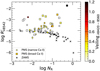 |
Fig. 5 Relationship between the Rossby number, NR, and the ratio of the surface flux of the chromospheric Ca II IRT emission line at 8542 Å to the stellar bolometric luminosity, R′. Circles represent PMS stars with narrow Ca II emission lines (<100 km s−1), while squares represent PMS stars with broad Ca II emission lines (>100 km s−1). Crosses denote ZAMS stars (Marsden et al. 2009; Yamashita & Itoh 2022). The color of the circles indicates the amount of veiling measured in 8420– 8560 Å. |
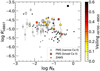 |
Fig. 6 Relationship between the ratio of the surface flux of the chromospheric Mg I emission line to the stellar bolometric luminosity, R′, and the Rossby number, NR. Large circles represent PMS stars with narrow Ca II emission lines (<100 km s−1), while squares represent PMS stars with broad Ca II emission lines (>100 km s−1). The color of the large circles and squares indicates the amount of veiling measured in 8700– 8850 Å. Dots represent PMS stars with no significant detection of the Mg I emission line. ZAMS stars examined in Yamashita & Itoh (2022) are shown as cross symbols. |
4.2.2 Chromospheric Mg I emission lines
Fig. 6 shows the ratio of the surface flux of the Mg I emission line at 8807 Å to the stellar bolometric luminosity, R′, as a function of the Rossby number. The PMS stars are compared with ZAMS stars examined in Yamashita & Itoh (2022), and are colored to represent the amount of veiling measured in 8700–8850 Å.
With the same Rossby number, some PMS stars have R′ values comparable to those of ZAMS stars, while others exhibit larger R′ values. The PMS stars without veiling show emission line strengths similar to those of ZAMS stars with the same Rossby numbers. The Mg I emission lines of such stars are considered to be formed by a dynamo process similar to that in ZAMS stars.
On the other hand, PMS stars with larger R′ than ZAMS stars with the same Rossby number, such as CV Cha and TWA 01, show veiling. More than half of these stars, including DK Tau, GQ Lup, and IQ Tau, also exhibit near-infrared excess, as is measured in Section 4.1, and broad Ca II emission lines with >100 km s−1. These objects are thought to possess protoplan- etary disks. For such stars, the chromosphere is activated not only by the dynamo process but also by mass accretion from a protoplanetary disk.
Veiling originates in the accretion shock column, which is generally divided into three subregions: the preshock region, the postshock (cooling) region, and the heated photosphere (Calvet & Gullbring 1998; Hartmann et al. 2016). The stellar photospheric pressure at the depth of continuum formation has been calculated as log g ≈ 3.5 ∼ 104 dyn cm−2, indicating that the shock forms near the photosphere (Calvet & Gullbring 1998). The Mg I emission lines are known to form from the lower chromosphere to the upper photosphere (Fleck et al. 1994), and it is considered that these emission lines are induced by accretion because the height where Mg I forms aligns with the shock region.
With the completion of this study, we propose using Mg I chromospheric emission lines as a new and effective method for examining the activity of fast-rotating PMS and ZAMS stars. Noyes et al. (1984) identified five observational indicators of the dynamo process: rotation, stellar mass, spectral type, convective zone thickness, and convective turnover time. They suggested that Rossby numbers, which incorporate these parameters, are a useful indicator of stellar activity for main-sequence stars.
We introduce mass accretion as an additional mechanism influencing chromospheric activity in PMS stars. Yamashita et al. (2020) studied Ca II emission lines in PMS stars and suggested that those with high mass accretion rates exhibit stronger Ca II emission lines than ZAMS stars. However, this conclusion was not strongly supported due to the saturation of R′ against the Rossby numbers. Yamashita & Itoh (2022) have demonstrated that Mg I emission lines are a good indicator of activity in fastrotating and active ZAMS stars. We conclude that Mg I emission lines are more suitable than Ca II emission lines for assessing chromospheric activity in active objects such as PMS stars.
5 Conclusions
We investigated the chromospheric activity of 64 G, K, and M-type PMS stars in four star-forming regions and seven moving groups. High-resolution optical spectra of these PMS stars were obtained using VLT/X-shooter and VLT/UVES, and the infrared Mg I (8807 Å) emission lines were examined. To detect the weak chromospheric emission lines, we first determined the atmospheric parameters (Teff and log g), projected rotational velocity, and veiling of each PMS star by comparing the observed spectra with photospheric model spectra. After subtracting the photospheric model spectrum from the PMS spectrum, Mg I emission lines were detected. For PMS stars with no veiling, the strengths of the Mg I emission lines are comparable to those of ZAMS stars with similar Rossby numbers. These lines are believed to form through a dynamo process similar to that in ZAMS stars. In contrast, PMS stars with veiling exhibit stronger Mg I emission lines than ZAMS stars. These stars are likely surrounded by pro- toplanetary disks, where mass accretion generates shocks near the photosphere, heating the chromosphere. We propose that the chromosphere of PMS stars is activated not only by the dynamo process but also by mass accretion.
Acknowledgements
This work would not have been possible without the financial support of the Japan Society for the Promotion of Science (JSPS) KAKENHI grant number 23KJ1855. M.Y. is also supported as a JSPS Research Fellow (DC2 and PD). We would like to thank Prof. Jung and Prof. Kim for providing the numerical results of the evolution tracks from Jung & Kim (2007) through private communication (see Fig. 3). This paper includes data collected with the TESS mission, from the Mikulski Archive for Space Telescopes (MAST) data archive at the Space Telescope Science Institute (STScI).
Appendix A Figures and tables
Physical parameters of 64 PMS stars.
Details of the archive data of VLT/X-shooter and VLT/UVES
Luminosity, temperature, surface gravity, and veiling values of 64 PMS stars
Projected rotational velocity (v sin i) derived by the previous study, period measured from TESS light curves, stellar age, mass, convective turnover time (τc), and Rossby number (NR) of the 64 PMS stars.
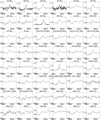 |
Fig. A.1 Mg I (8807 Å) emission lines of the 48 PMS stars. Continuum is normalized to unity. Photospheric absorption lines are already subtracted. |
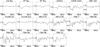 |
Fig. A.2 Spectra near Mg I (8807 Å) emission lines of the 16 PMS stars without significant detection. Continuum is normalized to unity. Photospheric absorption lines are already subtracted. |
EQWs, FWHMs, and R′ of the chromospheric emission lines of Ca II IRT (8542 Å), and Mg I (8807 Å). The EQW values in parentheses indicate non-significant.
References
- Bailer-Jones, C. A. L., Rybizki, J., Fouesneau, M., Mantelet, G., & Andrae, R. 2018, ApJ, 156, 58 [Google Scholar]
- Basri, G., & Batalha, C. 1990, ApJ, 363, 654 [Google Scholar]
- Batalha, C. C., & Basri, G. 1993, ApJ, 412, 363 [NASA ADS] [CrossRef] [Google Scholar]
- Batalha, C. C., Stout-Batalha, N. M., Basri, G., & Terra, M. A. O. 1996, ApJS, 103, 211 [NASA ADS] [CrossRef] [Google Scholar]
- Bessell, M. S., & Brett, J. M. 1988, PASP, 100, 1134 [Google Scholar]
- Blanco-Cuaresma, S., Soubiran, C., Heiter, U., & Jofre, P. 2014, A&A, 569, A111 [NASA ADS] [CrossRef] [EDP Sciences] [Google Scholar]
- Calvet, N., & Gullbring, E. 1998, ApJ, 509, 802 [Google Scholar]
- Cohen, J. G., Persson, S. E., Elias, J. H., & Frogel, J. A. 1981, ApJ, 249, 481 [NASA ADS] [CrossRef] [Google Scholar]
- Cutri, R. M., Skrutskie, M. F., van Dyk, S., et al. 2003, VizieR Online Data Catalog: II/246 [Google Scholar]
- Da Rio, N., Robberto, M., Hillenbrand, L. A., Henning, T., & Stassun, K. G. 2012, ApJ, 748, 14 [Google Scholar]
- Dunn, R. B., Evans, J. W., Jefferies, J. T., et al. 1968, ApJS, 15, 275 [NASA ADS] [CrossRef] [Google Scholar]
- Fleck, B., Deubner, F.-L., Maier, D., & Schmidt, W. 1994, IAU Symp., 154, 65 [NASA ADS] [Google Scholar]
- Frasca, A., Biazzo, K., Alcala, J. M., et al. 2017, A&A, 602, A33 [NASA ADS] [CrossRef] [EDP Sciences] [Google Scholar]
- Frohlich, C., & Lean, J. 2004, A&AR, 12, 273 [CrossRef] [Google Scholar]
- Fukugita, M., Ichikawa, T., Gunn, J. E., et al. 1996, ApJ, 111, 1748 [Google Scholar]
- Furlan, E., Watson, D. M., McClure, M. K., et al. 2009, ApJ, 703, 1964 [Google Scholar]
- Gaia Collaboration (Brown, A. G. A., et al.) 2021, A&A, 649, A1 [NASA ADS] [CrossRef] [EDP Sciences] [Google Scholar]
- Ghez, A. M., Neugebauser, G., & Matthews, K. 1993, ApJ, 106, 2005 [CrossRef] [Google Scholar]
- Glebocki, R., & Gnacinski, P. 2005, VizieR Online Data Cat, 3244 [Google Scholar]
- Gontcharov, G. A., & Mosenkov, A. V. 2017, MNRAS, 472, 3805 [NASA ADS] [CrossRef] [Google Scholar]
- Gray, D. F. 2005, The Observation and Analysis of Stellar Photospheres, 3rd edn. (Cambridge) [Google Scholar]
- Hamann, F., & Persson, S. E. 1992, ApJS, 82, 247 [NASA ADS] [CrossRef] [Google Scholar]
- Hartmann, L., Herczeg, G., & Calvet, N. 2016, ARA&A, 54, 135 [Google Scholar]
- Herczeg, G. J., & Hillenbrand, L. A. 2014, ApJ, 786, 97 [Google Scholar]
- Hosoya, K, Itoh, Y., Oasa, Y., Gupta, R., & Sen, A. K. 2019, Int. J. Astron. Astrophys., 09, 154 [NASA ADS] [CrossRef] [Google Scholar]
- James, D. J., & Jeffries, R. D. 1997, MNRAS, 291, 252 [NASA ADS] [CrossRef] [Google Scholar]
- Jones, A., Noll, S., Kausch, W., Szyszka, C., & Kimeswenger, S. 2013, A&A, 560, A91 [NASA ADS] [CrossRef] [EDP Sciences] [Google Scholar]
- Jung, Y. K., & Kim, Y.-C. 2007, J. Astron. Space Sci., 24, 1 [NASA ADS] [CrossRef] [Google Scholar]
- Kenyon S. J., Hartmann L., Strom K. M., & Strom S. E. 1990, AJ, 99, 869 [NASA ADS] [CrossRef] [Google Scholar]
- Kenyon S. J., Gomez M., Marzke R. O., Hartmann L. 1994, AJ, 108, 251 [NASA ADS] [CrossRef] [Google Scholar]
- Kraus, S., Hofmann, K.-H., Malbet, F., et al. 2009, A&A, 508, 787 [NASA ADS] [CrossRef] [EDP Sciences] [Google Scholar]
- Kraus, A. L., Ireland, M. J., Hillenbrand, L. A., & Martinache, F. 2012, ApJ, 745, 19 [Google Scholar]
- Kulenthirarajah, L., Donati, J. F., Hussain, G., Morin, J., & Allard, F. 2019, MNRAS, 487, 1335 [CrossRef] [Google Scholar]
- Leinert, C., Zinnecker, H., Weitzel, N., et al. 1993, A&A, 278, 129 [NASA ADS] [Google Scholar]
- Mamajec, E. E., Lawson, W. A., & Feigelson, E. D. 2000, ApJ, 544, 356 [NASA ADS] [CrossRef] [Google Scholar]
- Marsden, S. C., Carter, B. D., & Donati, J.-F. 2009, MNRAS, 399, 888 [NASA ADS] [CrossRef] [Google Scholar]
- Meyer, M., Calvet, N., & Hillenbrand, L. 1997, AJ, 114, 288 [NASA ADS] [CrossRef] [Google Scholar]
- Michel, A., van der Marel, N., & Matthews, B. C. 2021, ApJ, 921, 72 [CrossRef] [Google Scholar]
- Mohanty, S., Jayawardhana, R., & Basri, G. 2005, ApJ, 626, 498 [NASA ADS] [CrossRef] [Google Scholar]
- Mullan, D. J. 1973, ApJ, 186, 105 [Google Scholar]
- Muzerolle, J., Hartmann, L., & Calvet, N. 1998, ApJ, 116, 455 [CrossRef] [Google Scholar]
- Neuhauser, R., Strerzik, M. F., Schmitt, J. H. M. M., Wichmann, R., & Krautter, J. 1995, A&A, 297, 391 [NASA ADS] [Google Scholar]
- Noll, S., Kausch, W., Barden, M., et al. 2012, A&A, 543, A92 [NASA ADS] [CrossRef] [EDP Sciences] [Google Scholar]
- Noyes, R. W., Hamann, F. W., Baliunas, S. L., & Vaughan, A. H. 1984, AJ, 279, 763 [NASA ADS] [CrossRef] [Google Scholar]
- Palacios, A., Gebran, M., Josselin, E., et al. 2010, A&A 516, A13 [NASA ADS] [CrossRef] [EDP Sciences] [Google Scholar]
- Rebull, L. M., Stauffer, J. R., Bouvier, J., et al. 2016, AJ, 152, 113 [Google Scholar]
- Scargle, J. D. 1982, AJ, 263, 835 [Google Scholar]
- Soderblom, D. R., Stauffer, J. R., & Hudon, J. D. 1993, ApJ, 85, 315 [NASA ADS] [Google Scholar]
- Takeda, Y., Ohkubo, M., Sato, B., Kambe, E., & Sadakane, K. 2005, PASJ, 57, 27 [NASA ADS] [CrossRef] [Google Scholar]
- Tonry, J. L., Denneau, L., Flewelling, H., et al. 2018, ApJ, 867, 105 [NASA ADS] [CrossRef] [Google Scholar]
- Uchida, Y., & Shibata, K. 1985, PASJ, 37, 515 [NASA ADS] [Google Scholar]
- van de Hulst, H. C., 1968, Nebulae and Interstellar Matter [Google Scholar]
- Vernazza, J. E., Avrett, E. H., & Loeser, R. 1981, ApJS, 45, 635 [Google Scholar]
- Wahhaj, Z., Cieza, L., Koerner, D. W., et al. 2010, ApJ, 724, 835 [Google Scholar]
- Yamashita, M., & Itoh, Y. 2022, PASJ, 74, 557 [NASA ADS] [CrossRef] [Google Scholar]
- Yamashita, M., Itoh, Y., & Takagi, Y. 2020, PASJ, 72, 80 [NASA ADS] [CrossRef] [Google Scholar]
- Yang, H., Herczeg, G. J., Linsky, J. L., et al. 2012, ApJ, 744, 121 [NASA ADS] [CrossRef] [Google Scholar]
- Yu, J., Khanna, S., Themessl, N., et al. 2023, ApJS, 264, 41 [NASA ADS] [CrossRef] [Google Scholar]
- Zacharias, N., Finch, C. T., Girard, T. M., et al. 2013, ApJ, 145, 1 [Google Scholar]
- Zuckerman, B., & Song, I. 2004, A&A, 42, 685 [NASA ADS] [CrossRef] [Google Scholar]
The details are described in the webpage of National Aeronautics and Space Administration, NASA; https://heasarc.gsfc.nasa.gov/docs/tess/LightCurveFile-Object-Tutorial.html
IRAF software is distributed by the National Optical Astronomy Observatories, which are operated by the Association of Universities for Research in Astronomy, Inc., under a cooperative agreement with the National Science Foundation.
All Tables
Projected rotational velocity (v sin i) derived by the previous study, period measured from TESS light curves, stellar age, mass, convective turnover time (τc), and Rossby number (NR) of the 64 PMS stars.
EQWs, FWHMs, and R′ of the chromospheric emission lines of Ca II IRT (8542 Å), and Mg I (8807 Å). The EQW values in parentheses indicate non-significant.
All Figures
|
Fig. 1 Procedure for subtracting the photospheric component from PMS star spectra. The top portion of each panel shows the observed spectrum (solid line), while the model spectrum is represented by the dashed line. For display purposes, the spectra of the PMS stars and the models are shifted by +1.0 or +2.0. The bottom portion of each panel displays the difference between the PMS star spectrum and the model spectrum. Hatched areas indicate Fe I, Ca II, and Mg I lines. Wavelengths within these hatched areas have been excluded from the fitting range. |
| In the text | |
|
Fig. 2 Comparison between the effective temperature determined in this study and that derived from the spectroscopic study of Frasca et al. (2017). |
| In the text | |
|
Fig. 3 HR diagram of the investigated PMS stars. The solid and dashed lines denote the evolutionary tracks (0.065–4.5 M⊙) and isochrones (2 × 10⁵ yr to the main sequence) of Jung & Kim (2007). We linearly interpolated that model to one tenth of the original. The thick solid line denotes the evolutionary track for a 1 M⊙ star. The circles represent the PMS stars. |
| In the text | |
|
Fig. 4 Near-infrared color-color diagram for the PMS stars we investigated. Circles denote the PMS stars, with the color indicating the amount of veiling measured in 8798–8802 and 8813–8819 Å. The dash- dotted lines represent the linear least-squares fit to the intrinsic color of the CTTSs (Meyer et al. 1997). Intrinsic colors for main-sequence stars (solid line) and giant stars (dashed line) are from Bessell & Brett (1988). B.G. stands for background star. The arrow and dotted lines show the interstellar reddening vector from Cohen et al. (1981). |
| In the text | |
|
Fig. 5 Relationship between the Rossby number, NR, and the ratio of the surface flux of the chromospheric Ca II IRT emission line at 8542 Å to the stellar bolometric luminosity, R′. Circles represent PMS stars with narrow Ca II emission lines (<100 km s−1), while squares represent PMS stars with broad Ca II emission lines (>100 km s−1). Crosses denote ZAMS stars (Marsden et al. 2009; Yamashita & Itoh 2022). The color of the circles indicates the amount of veiling measured in 8420– 8560 Å. |
| In the text | |
|
Fig. 6 Relationship between the ratio of the surface flux of the chromospheric Mg I emission line to the stellar bolometric luminosity, R′, and the Rossby number, NR. Large circles represent PMS stars with narrow Ca II emission lines (<100 km s−1), while squares represent PMS stars with broad Ca II emission lines (>100 km s−1). The color of the large circles and squares indicates the amount of veiling measured in 8700– 8850 Å. Dots represent PMS stars with no significant detection of the Mg I emission line. ZAMS stars examined in Yamashita & Itoh (2022) are shown as cross symbols. |
| In the text | |
|
Fig. A.1 Mg I (8807 Å) emission lines of the 48 PMS stars. Continuum is normalized to unity. Photospheric absorption lines are already subtracted. |
| In the text | |
|
Fig. A.2 Spectra near Mg I (8807 Å) emission lines of the 16 PMS stars without significant detection. Continuum is normalized to unity. Photospheric absorption lines are already subtracted. |
| In the text | |
Current usage metrics show cumulative count of Article Views (full-text article views including HTML views, PDF and ePub downloads, according to the available data) and Abstracts Views on Vision4Press platform.
Data correspond to usage on the plateform after 2015. The current usage metrics is available 48-96 hours after online publication and is updated daily on week days.
Initial download of the metrics may take a while.