| Issue |
A&A
Volume 595, November 2016
|
|
|---|---|---|
| Article Number | A121 | |
| Number of page(s) | 8 | |
| Section | The Sun | |
| DOI | https://doi.org/10.1051/0004-6361/201628277 | |
| Published online | 11 November 2016 | |
Near-Sun and 1 AU magnetic field of coronal mass ejections: a parametric study
1 University of Ioannina, Department of Physics, Section of Astrogeophysics, 45110 Ioannina, Greece
e-mail: This email address is being protected from spambots. You need JavaScript enabled to view it.
2 Research Center for Astronomy and Applied Mathematics, Academy of Athens, Athens, Greece
Received: 8 February 2016
Accepted: 3 August 2016
Abstract
Aims. The magnetic field of coronal mass ejections (CMEs) determines their structure, evolution, and energetics, as well as their geoeffectiveness. However, we currently lack routine diagnostics of the near-Sun CME magnetic field, which is crucial for determining the subsequent evolution of CMEs.
Methods. We recently presented a method to infer the near-Sun magnetic field magnitude of CMEs and then extrapolate it to 1 AU. This method uses relatively easy to deduce observational estimates of the magnetic helicity in CME-source regions along with geometrical CME fits enabled by coronagraph observations. We hereby perform a parametric study of this method aiming to assess its robustness. We use statistics of active region (AR) helicities and CME geometrical parameters to determine a matrix of plausible near-Sun CME magnetic field magnitudes. In addition, we extrapolate this matrix to 1 AU and determine the anticipated range of CME magnetic fields at 1 AU representing the radial falloff of the magnetic field in the CME out to interplanetary (IP) space by a power law with index αB.
Results. The resulting distribution of the near-Sun (at 10 R⊙) CME magnetic fields varies in the range [0.004, 0.02] G, comparable to, or higher than, a few existing observational inferences of the magnetic field in the quiescent corona at the same distance. We also find that a theoretically and observationally motivated range exists around αB = −1.6 ± 0.2, thereby leading to a ballpark agreement between our estimates and observationally inferred field magnitudes of magnetic clouds (MCs) at L1.
Conclusions. In a statistical sense, our method provides results that are consistent with observations.
Key words: Sun: atmosphere / Sun: coronal mass ejections (CMEs) / Sun: magnetic fields / solar-terrestrial relations
© ESO, 2016
1. Introduction
Knowledge of the magnetic field entrained in coronal mass ejections (CMEs) is a crucial parameter for their energetics, dynamics, structuring, and eventually of their geoeffectiveness. For instance, the overall CME energy budget is dominated by the energy stored in non-potential magnetic fields (e.g., Forbes 2000; Vourlidas et al. 2000). In addition, given that CMEs and interplanetary (IP) counterparts (interplanetary CMEs (ICMEs)) are magnetic configurations with a low-β plasma parameter, their structural evolution as they propagate and expand into the IP space is dictated by the balance and interactions between their magnetic field and the ambient solar wind (e.g., Démoulin & Dasso 2009). Moreover, upon arrival at 1 AU, the magnitude of the southward magnetic field of earth-directed interplanetary CMEs (ICMEs) is the most important parameter determining their geoeffectiveness (e.g., Wu & Lepping 2005). Therefore, the near-Sun magnetic field magnitude is a key parameter for both space weather studies and applications, for example, by constraining the properties of coronal flux ropes ejected into the IP medium (e.g., Shiota & Kataoka 2016), and in anticipation of the observations of upcoming solar and heliospheric missions. Unfortunately, very few direct observational inferences of near-Sun (~1−7 R⊙) CME magnetic fields exist currently (e.g., Bastian et al. 2001; Jensen & Russell 2008; Tun & Vourlidas 2013). These are based on relatively rare radio emission configurations, such as gyrosynchrotron emission from CME cores and Faraday rotation, and require detailed physical modeling of relevant radio emission processes to infer the magnetic field that is sought after.
We recently proposed a new method to deduce the near-Sun magnetic field magnitude (hereafter, magnetic field) of CMEs (Patsourakos et al. 2016). This method relies on the conservation of magnetic helicity in cylindrical flux ropes and uses as inputs the magnetic helicity budget of the source region and geometrical parameters (length and radius) of the associated CME. It supplies an estimation of the near-Sun CME magnetic field which is then extrapolated to 1 AU using a power-law fall-off dictated by the radial (heliocentric) distance. We have successfully applied this method to a major geoeffective CME launched from the Sun on 7 March 2012, which triggered one of the most intense geomagnetic storms of solar cycle 24. Recently, two other methods to infer the CME-ICME magnetic field vectors were proposed (Kunkel & Chen 2010; Savani et al. 2015). Kunkel & Chen (2010) use a flux-rope CME model, driven by poloidal magnetic flux injection, which is constrained by the height-time profile of the associated CME. The Savani et al. (2015) method is based on the heliospheric magnetic helicity rule, the tilt of the source active region (AR), and the magnetic field strength of the compression region around the CME.
In this work we perform a parametric study of the method to assess its robustness before applying it to observed cases. We essentially use distributions of input parameters derived from observations to determine the near-Sun and 1 AU magnetic fields for a set of synthetic CMEs. This study offers statistics sufficient to determine the range of the anticipated CME magnetic fields both near-Sun and at 1 AU. The latter distribution is compared to actual magnetic-cloud (MC) observations at 1 AU.
In the following, Sect. 2 describes how we infer the near-Sun CME magnetic field, while Sect. 3 describes how this value is extrapolated to 1 AU. Section 4 describes our parametric study, Sect. 5 includes some further tests and uncertainty estimations, while Sect. 6 summarizes our results, their limitations, and an outlook for future revisions.
2. The helicity-based method to infer the near-Sun magnetic field of CMEs
2.1. Theory
We use the Lundquist flux-rope model (Lundquist 1950) as a typical IP prescription of propagating MCs. This is an axisymmetric force-free solution with components expressed in cylindrical coordinates (r,φ,z) as  (1)where J0 and J1 are the Bessel functions of the zeroth and first kind, respectively, σH = ± 1 is the helicity sign (i.e., handedness), α is the (constant) force-free parameter, and B0 is the maximum (axial) magnetic field. The standard assumption that the first zero of J0 occurs at the edge of the flux rope (e.g., Lepping et al. 1990) is made here, namely
  (2)with R corresponding to the flux-rope radius. This assumption leads to a purely axial or azimuthal magnetic field at the flux-rope axis or edge.
Following Eq. (9) of Dasso et al. (2006), the magnetic helicity Hm of a Lundquist flux rope is written as  (3)where L is the flux-rope length. The CME magnetic field distribution at 15 R⊙ from an 2.5D MHD simulation was found to be in excellent agreement with the Lundquist model described above (see Fig. 8 in Lynch et al. 2004).
Solution of the above equation for the unknown axial magnetic field B0, with the aid of Eq. (2), gives  (4)with
  (5)Hence, the parameters determining B0, via the application of Eqs. (2), (4), and (5), in this case are the length L and radius R of the flux-rope CME along with its magnetic helicity content, Hm.
2.2. Observational constraints to determine the near-Sun CME magnetic field magnitude
From the analysis of the previous section, one needs to know a set of magnetic and geometrical properties of a CME to calculate the axial magnetic field B0. In this section we discuss how to deduce estimates of these parameters from observations.
To infer the magnetic helicity content Hm of a CME, one needs to first calculate the coronal helicity content of the solar source region. This is achieved in various ways. These methods typically use photospheric, mainly vector, magnetograms and are based on various theoretical setups, including the calculation of the magnetic helicity-injection rate from photospheric motions (Pariat et al. 2006), partitioning of the photospheric flux into assumed slender flux tubes and calculation of the connectivity matrix to deduce the total helicity (Georgoulis et al. 2012), and classical volume calculations on coronal magnetic field extrapolations (Régnier & Canfield 2006; Valori et al. 2012; Moraitis et al. 2014, among others). Detailed descriptions of the different methods can be found in the above works.
To obtain the geometrical parameters R and L we use the graduated cylindrical shell (GCS) forward fitting model of Thernisien et al. (2009). This is a geometrical flux-rope model routinely used to fit the large-scale appearance of flux-rope CMEs in multi-viewpoint observations acquired by the coronagraphs on board the Solar and Heliospheric Observatory (SOHO) and Solar Terrestrial Relations Observatory (STEREO) spacecraft. The GCS user modifies a set of free geometrical (front height H, half-angular width w, aspect ratio k, and tilt angle) and positional (central longitude and latitude) parameters of the flux-rope CME until a satisfactory agreement is achieved between the model projections and the actual observations. A detailed description can be found in Thernisien et al. (2009).
In the framework of the GCS model, the CME radius R at a heliocentric distance r is  (6)To assess the flux-rope length L, it is assumed that the CME front is a cylindrical section (see Fig. 1 of Démoulin & Dasso 2009) with an angular width provided by the geometrical fitting. One may then write
  (7)where rmid( = H−R) is the heliocentric distance halfway through the model’s cross section, along its axis of symmetry. The half-angular width w is given in radians.
It is important to realize that the source-region determinations of magnetic helicity, including estimates of the CME helicity content Hm, correspond to the photosphere or low corona, while those for R and L refer to the outer corona, which are typically a few solar radii in heliocentric distance. To allow the use of this Hm we adhere to the well-documented conservation principle of magnetic helicity (Berger 1984, 1999). Indeed, for a magnetized plasma with a high magnetic Reynolds number, as the solar corona is widely believed to be, the relative magnetic helicity is conserved even in case of magnetic reconnection; for a recent, successful test of the conservation principle, see Pariat et al. (2015). Assuming that an ascending CME in the solar corona does not accumulate substantial overlying magnetic structures that drastically modify its magnetic helicity content, we use its estimated low-coronal Hm up to the outer corona.
Summarizing, estimates of R, L, and Hm allow us to estimate an upper limit of the near-Sun axial magnetic field B0 of flux-rope CMEs at distances covered by coronagraphs.
3. Extrapolation of the near-Sun CME magnetic field magnitude to 1 AU
To extrapolate the near-Sun CME magnetic-field magnitude B∗, determined at a heliocentric distance r∗ (Sect. 2), to 1 AU, we assume that its radial evolution follows a power-law behavior of the form  (8)with r corresponding to the heliocentric distance. In Eq. (8) we assume that the power-law index αB varies in the range [− 2.7, − 1.0]. This is a typical approximation that is frequently followed in the literature (e.g., Patzold et al. 1987; Kumar & Rust 1996; Bothmer & Schwenn 1998; Vršnak et al. 2004; Liu et al. 2005; Forsyth et al. 2006; Leitner et al. 2007; Démoulin & Dasso 2009; Poomvises et al. 2012; Mancuso & Garzelli 2013; Winslow et al. 2015; Good & Forsyth 2016). These theoretical and observational studies also roughly determine the range of αB values used here. Most of these studies do not fully cover the range (i.e., [10 R⊙, 1 AU]) we are considering here, but typically subsets thereof, either near-Sun or inner heliospheric.
4. Parametric study
The parameterization of our method consists of the following steps:
-
1.
We randomly select a magnetic helicity valueHm resulting from a distribution of 162 active-region helicity values at different times, corresponding to 42 different solar ARs (Tziotziou et al. 2012). The selected active-region helicity is then assigned to a synthetic CME, therefore assuming for simplicity, that the CME is fully extracting its source region helicity. Given the ample dynamical range of the helicity values in the above study (at least three orders of magnitude), even assigning a fraction of each active-region helicity value to model the CME helicity would not lead to remarkably different statistical results.
-
2.
We randomly select CME aspect ratios and angular widths from distributions resulting from the forward modeling of 65 CMEs observed by the STEREO coronagraphs (Thernisien et al. 2009; Bosman et al. 2012). The observations correspond to a distance of 10 R⊙, therefore supplying near-Sun geometric properties of the observed CMEs. The GCS model of Thernisien et al. (2009), described in Sect. 2, was used in the analysis of these observations. The deduced CME aspect ratios and angular widths take values in the intervals [0.09, 0.7] and [6, 41] deg, respectively. We then deduce the corresponding radii R and lengths L from Eqs. (6) and (7), respectively.
-
3.
From the above information, we calculate a near-Sun CME magnetic field B∗ at r∗ = 10R⊙ (Eq. (4)).
-
4.
For the B∗ calculated in step 3, and for each of the 18 equidistant values with a step equal to 0.1 covering the αB range ([− 2.7, − 1.0]) described in the previous section, we determine 18 CME magnetic field (B1 AU) values at r = 1 AU from Eq. (8).
-
5.
We repeated 104 times the process of randomly selecting Hm, R, and L to get a corresponding B∗ (steps 1−3). This supplied sufficient statistics to build a database of synthetic CMEs. The combination of the 104 near-Sun CME magnetic field values with the 18 different αB values gave rise to 180 000 total values of the CME magnetic field at 1 AU.
In essence, the above parameterization provides 104 near-Sun CME magnetic fields B∗ and, out of those, 1.8 × 10⁵ ICME magnetic fields B1 AU at 1 AU.
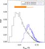 |
Fig. 1 Probability density functions of the derived near-Sun CME magnetic fields for 104 synthetic CMEs in two different cases: using the sample of all (eruptive and non-eruptive) active-region relative magnetic helicity budgets Hm (black histogram) and using only the subsample of eruptive active-region helicity budgets (blue histogram). The horizontal orange bar shows the range of various observational estimates for the magnetic field of the quiescent (i.e., noneruptive) solar corona. In all cases, the estimates correspond to a heliocentric distance of 10 R⊙. |
In Fig. 1 we show the probability density function (PDF) of the derived near-Sun CME magnetic fields B∗ at r∗ = 10R⊙ in two different situations: using all active-region helicity values of Tziotziou et al. (2012; black histogram) and using only the active-region helicity values of eruptive regions (i.e., hosting flares of GOES class M1.0 and above), in which case these values exceed 2 × 1042 Mx2 (blue histogram). In the first case, the PDF peaks at ≈0.007 G and has a full width at half maximum (FWHM) range at roughly [0.004, 0.03] G. The distribution is asymmetric, showing an extended B∗ tail. In the second case, the PDF peaks at higher values, ~0.03 G, and presents a FWHM at roughly [0.02, 0.06] G. This distribution corresponds to ARs that are known to be more prone to eruptions (e.g., Andrews 2003; Nindos et al. 2015). Weaker flares do not necessarily mean lower helicity budgets as an eruptive AR with substantial magnetic helicity can give a series of eruptive C-class flares along with M- and, possibly, X-class flares.
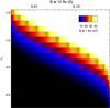 |
Fig. 2 Color-coded range of the derived B1 AU (nT) as a function of the near-Sun CME magnetic field B0 at 10 R⊙ (abscissa) and of the power-law exponent αB of the radial CME-ICME falloff (ordinate). The color scale is saturated such that white and black areas lie outside the observed MC magnetic fields by WIND observations at L1. |
There are a few observational inferences of the coronal magnetic field at 10 R⊙. They rely on techniques such as Faraday rotation and CME-shock stand-off distance and give magnetic field strengths in the range [0.009−0.02] G (e.g., Bemporad & Mancuso 2010; Gopalswamy & Yashiro 2011; Kim et al. 2012; Poomvises et al. 2012; Mancuso & Garzelli 2013; Susino et al. 2015). They mainly correspond to observations in the quiescent corona and are represented by the orange horizontal bar in Fig. 1. A significant fraction of the synthetic CMEs have magnetic fields comparable to or higher than those corresponding to the quiescent corona. The latter is essentially the case for the subset of synthetic CMEs that correspond to prone-to-erupt ARs. Our results are thus consistent with the notion that CMEs are structures with stronger magnetic fields than the quiescent ambient corona.
A context representation of the extrapolated CME-ICME magnetic fields at 1 AU, B1 AU, for the 180 000 considered cases, is given in Fig. 2. Here we use a color representation of B1 AU as a function of B∗ and αB. The color scaling has been saturated so that B∗ values outside the range of magnetic field magnitudes in observed magnetic clouds (MCs) at 1 AU, namely BMC ∈ [ 4,45 ] nT, are shown in either black (smaller) or white (higher). Any other color corresponds to projected B∗ values within the observed BMC range. The distribution of BMC results from linear force-free fits of 162 MCs observed in situ at 1 AU by WIND (Lynch et al. 2003; Lepping et al. 2006). Several remarks can be made from this image. First, there is a significant number of cases, i.e., (B∗−αB) pairs, resulting in B1 AU values outside the observed BMC range. This suggests that the corresponding parameter space can be significantly constrained. Second, B1 AU seems to depend more sensitively on αB than on B∗. This can be assessed from Fig. 2 by noting that while the vertical colored (i.e., not black and white) bands corresponding to a given B∗ in agreement with the observed BMC range show more or less the same extent, this is not the case for the horizontal colored bands corresponding to a given αB. In this latter case, we also notice very narrow bands at both ends of the employed αB range.
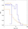 |
Fig. 3 Probability density function of the extrapolated to 1 AU magnetic fields of 10 000 synthetic CMEs (orange histogram). These functions correspond to the full range of the considered αB values, i.e., 180 000 B1 AU values in total. This is compared with the probability density function of the magnetic-field magnitude for 162 MCs observed in situ at 1 L1 by WIND (blue histogram). |
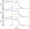 |
Fig. 4 Probability density functions of the extrapolated to 1 AU magnetic field for 10 000 synthetic CMEs (orange histogram). The probability density functions correspond to αB equal to − 2.6 (top plot), − 1.6 (middle plot), and − 1.2 (bottom plot). All cases are compared with the PDF of the magnetic field magnitude for 162 magnetic observed in situ at L1 by WIND (blue histogram). |
To better understand the B1 AU sensitivity on αB we perform the following further tests. In Fig. 3 we show the histogram of B1 AU (orange curve) corresponding to the full range of the considered αB values, which is overplotted on the histogram of BMC (blue curve). It is then clear that the two histograms do not match, even saliently. This suggests that not all employed αB values yield consistent results, which is in line with the result of Fig. 2.
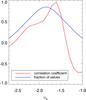 |
Fig. 5 Correlation coefficient of the probability density functions for the predicted B1 AU and observed BMC values at L1 as a function of αB (red curve). Also shown is the respective fraction of B1 AU values (blue curve) falling within the observed BMC range. |
In Fig. 4 we show the B1 AU histograms corresponding to three different, specific values of αB. These values were meant to represent the two extremes of the αB distribution, but also a value maximizing the reproduction of BMC by B1 AU. Radial falloffs of the CME-ICME magnetic field that are too steep (αB = −2.6; top plot) or too shallow (αB = −1.2; bottom plot) give rise to B1 AU values that are too low and too high, respectively, compared with the MC observations. On the other hand, setting αB = −1.6 (middle plot) we obtain a fair agreement between the predicted and observed CME magnetic fields at 1 AU, at least for the bulk of the distribution. Both distributions peak around 10 nT and have similar FWHM of ~15 nT. However, the modeled distribution has a high-B tail that is not present in the MC observations. A similar value for αB was found in an application of the method to a single event (Patsourakos et al. 2016).
Clearly, there is a range of αB values around − 1.6 that yields results that are consistent with MC observations. We produced Fig. 5 to firmly establish this interval and quantify its merit. In this test we show the linear correlation coefficient (red curve) between BMC and B1 AU histograms as a function of αB, thus obtaining 18 values of this correlation coefficient. We find that the correlation coefficient exhibits a well-defined peak around 0.9 at αB = −1.6 and stays above 0.5 when αB ∈ [− 1.9,− 1.5]. Very small or even negative correlation coefficients are found when αB moves toward extreme values of its assumed range.
Another useful measure of best-fit αB values is provided by the fraction of the predicted values B1 AU agreeing with the range of BMC values as a function of αB. This is shown by the blue curve in Fig. 5. The peak of this fraction occurs at 0.8 (80%) for a slightly different αB value (− 1.9) compared to the peak of the correlation coefficient (− 1.6). Nonetheless, the fraction is above 0.5 (50%) for αB ∈ [− 1.9, − 1.5]. The relative discrepancy between the peaks of the two curves in Fig. 5 is not unexpected. Indeed, the correlation coefficient measures the degree of overlap between the two distributions, while the fraction denotes the subset of points within a given range with no a priori reason for the two distributions to match. Since both the fraction and correlation coefficient reach their maxima for αB ∈ [− 1.9, − 1.5], however, we consider this range as the best-fit range, as we are able to reproduce the observed BMC distribution relatively well and at the same time yield a significant number of cases within the BMC range.
5. Further tests and an uncertainty estimation for αB
An important issue, which is directly relevant to our analysis, is how the (input) AR helicity PDF relates to the MC helicity content at 1 AU. To investigate this, we constructed the PDF of the magnetic helicity of MCs observed at 1 AU (see also Lynch et al. 2005; and Démoulin et al. 2016, for MC Hm PDFs) and compared it with the AR helicities used in this study. We used the Lundquist linear force-free model, as in our analysis, to obtain MC helicities and applied this model to the MC fittings of Lynch et al. (2003) and Lepping et al. (2006). We used two different approaches for the MC lengths required in the Hm calculation. First, we used the results of in situ observations of near-relativistic electrons inside MCs, which can supply a proxy for their lengths, given their solar release times, onset times at 1 AU, and speeds (e.g., Larson et al. 1997). This is because near-relativistic electrons, assuming they propagate scatter-free, have small gyroradii and thus follow the magnetic field very closely. A statistical study of 30 near-relativistic events in 8 MCs gave an average MC length of 2.28 AU (Kahler et al. 2011). Second, we adopted the statistical approach of Démoulin et al. (2016). This study used the results of MC fittings of Lynch et al. (2003) and Lepping et al. (2006) and found that several MC properties, including their helicity per unit length, do not depend significantly on the position along the MC axis. This allowed the derivation of a generic shape for the MC axis, parameterized in terms of its angular span, which further enabled an estimation of the MC length assuming a rooting of both its legs in the Sun. The resulting average MC length was 2.6 AU. The average of the two MC-length estimates above, which we use for the remainder of this section, is 2.44 AU.
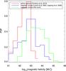 |
Fig. 6 Probability density functions of the Hm corresponding to (a) AR sample of Tziotziou et al. (2013; red histogram), (b) MC linear-force free fittings at 1 AU using the data from the Lynch et al. (2003) and Lepping et al. (2006) studies (blue histogram), and (c) B1 AU corresponding to the best-fit αB from this work (green histogram). |
We further constructed a helicity PDF for the synthetic MCs of this study. For this task we used the B1 AU values of these MCs, an average MC length of 2.44 AU, and an average MC radius of 0.11 AU, as obtained by Lynch et al. (2003) and Lepping et al. (2006). Figure 6 depicts the resulting MC Hm distribution from (i) the above literature studies (blue histogram); (ii) the source ARs (red histogram); and (iii) our synthetic MCs (green histogram). The maximum-likelihood values and FWHMs (in 1042 Mx2) of the three distributions are 6.3 and 5.3 for the AR Hm distribution; 6.3 and 13.3 for the literature work estimates; and 15.8 and 248.7 for the synthetic MC Hm of this study.
Clearly, our AR Hm distribution shows a deficit compared to both observed and synthetic MC Hm distributions. With respect to the observed MC distribution, this is not totally unexpected, as both AR and MC Hm calculations are model dependent, and possibly involve various systematic effects. For example, Tziotziou et al. (2013) calculated AR helicities using the Georgoulis et al. (2012) method that, by construction, infers a lower limit of AR free energies and the corresponding relative magnetic helicity. Different helicity calculation methods in ARs give rise to difference factors ranging between 1 and several (but less than 10) units. An analysis by Tziotziou et al. (in prep.), in particular, gave a difference factor of ~ 2.5, while Tziotziou et al. (2013) and Nindos & Andrews (2004) independently found average AR helicities on the order 6.6 × 1042Mx2 and 19.5 × 1042Mx2, which also differ by a factor of ~3. In addition, one cannot exclude the possibility that CMEs accumulate more helicity during their initial stages in the inner corona by poloidal magnetic flux addition via magnetic reconnection with their surroundings (e.g., Lin et al. 2004; Qiu et al. 2007) and, conversely, loose helicity in the inner heliosphere owing to magnetic erosion (e.g., Dasso et al. 2006; Gosling et al. 2007; Manchester et al. 2014; Ruffenach et al. 2015). Moreover, the flux-rope structure (i.e., twisted magnetic fields) may be confined only to the MC leading edge, (e.g., Owens 2016), suggesting that the employed magnetic field lengths in MC Hm calculations could represent upper limits. Finally, while different cylindrical MC models applied to the same data set lead to rather small differences in the resulting helicities (up to ~30%; Gulisano et al. 2005), departures from circular MC cross sections could lead to larger (by a factor 2−3) differences (Démoulin et al. 2016).
Comparing the synthetic and observed MC Hm distributions from Fig. 6, we see than the former corresponds to somewhat higher values compared to the latter. Given the significant overlap, however, we could say that the distributions are not dissimilar. Again, this is not totally unexpected because of systematic effects involved in calculations. In addition, these differences may be due to the fact that our method does not explicitly invoke the near-Sun-1 AU helicity conservation, however, a power-law formulation that has been introduced in line with many previous studies, but in a rather ad hoc manner.
Concluding, it seems reasonable to expect some differences in the statistical distributions of the AR and MC helicities. That said, several studies found an overall agreement, albeit with significant uncertainties, between the source region eruption-related and associated MC helicities (e.g., Green et al. 2002; Nindos et al. 2003; Luoni et al. 2005; Mandrini et al. 2005; Rodriguez et al. 2008; Kazachenko et al. 2012). This rough Hm conservation was found not only between the Sun and 1 AU, but also for a MC observed at 1 AU and at 5.4 AU (Nakwacki et al. 2011). Finally, statistical studies found that the Hm signs of the CME source regions matches those of associated MCs for up to 88% (Bothmer & Schwenn 1998; Cho et al. 2013). These studies underline the connection between the source region and MC Hm, at the same time shedding light on the significant uncertainties present in all stages of the calculations. This remains an objective for future efforts to narrow down and constrain the various uncertainties and modulations.
Further on, we briefly investigate the sensitivity of the near-Sun B0 value to the input AR helicity. This was achieved by overestimating and underestimating the AR Hm values by factors of 3 and 1/3, for reasons explained above. Factors 3 (1/3) give rise to higher (lower) near-Sun magnetic fields, and therefore steeper (shallower) radial falloffs of the CME magnetic field in the IP space are required in order to match the observed magnetic-field range in MCs. The values of the power-law index αB yielding a maximum correlation between the predicted and observed MC magnetic field are − 1.8 and − 1.4, respectively. These αB values correspond to rather small departures from the best-fit αB of − 1.6 and could thus serve as a measure of the uncertainty (± 0.2) of the best-fit αB.
6. Summary and discussion
Developing methods for the practical estimation of the magnetic field of CMEs, both near the Sun and at 1 AU, is a timely and important task for assessing the near-Sun energetics and dynamics of CMEs and for providing clues of the possible geoeffectiveness of their ICME counterparts. We recently developed one such method and we hereby perform a parametric study of it. Our study only applies to the CME magnetic-field magnitude and not its orientation, hence, reaching results pertinent to the CME geoeffectiveness requires an extension of this work. Our major conclusions are the following:
-
1.
The predicted near-Sun CME (at 10 R⊙) magneticfields (Fig. 1) exhibit a FWHM range of [0.004,0.03] G and their distribution shows values that arecomparable to, or higher than, magnetic fields measured in thequiescent corona by a handful of observations. For solar ARsources prone to eruptions, the FWHM of CME magnetic fields is[0.02, 0.07] G, which is clearly higher than the quiescent-coronamagnetic field at10 R⊙ (Fig. 1).
-
2.
The extrapolated CME-ICME magnetic field at 1 AU depends more sensitively on the power-law index αB of its radial dependence than on the near-Sun CME magnetic fields (Fig. 2).
-
3.
Considering the full range of literature-suggested αB values ([− 2.7, − 1.0]), we find that the extrapolated near-Sun magnetic fields at 1 AU do not match MC magnetic-field measurements (Fig. 3).
-
4.
For αB varying in the range [− 1.9, − 1.4], we obtain a considerable ballpark agreement with MC magnetic-field measurements at 1 AU in terms of both the similarity of the corresponding distributions and the high fraction of B1 AU values falling within the BMC value range. A best-fit αB attains a value of − 1.6 (Figs. 4, 5).
Statistically, therefore, our method is able to reproduce the ballpark of the ICME magnetic field magnitudes at 1 AU reasonably well. This result encourages us to seek further opportunities to apply the method to observed CME cases in the future. Interestingly, the best-fit αB = −1.6 stems independently from the analytical model of Démoulin & Dasso (2009), which treats CMEs as expanding force-free magnetic flux ropes in equilibrium with the total pressure of the ambient solar wind.
In the following, we summarize our assumptions and simplifications that could represent areas of future method improvements. We used AR helicity values taken from Tziotziou et al. (2012), which were calculated via the Georgoulis et al. (2012) method. Several methods exist to calculate Hm (Sect. 2.1). Application of these methods to the same data set, i.e., a sequence of HMI vector magnetograms, spanning over a two-day period (6−7) of March 2012 for the supereruptive NOAA AR 11429, showed that the Hm determinations, even though they stem from very different methods, show an overall agreement within a factor ~ 2.5 (Tziotziou et al., in prep.). In addition, while the employed Hm values refer to entire ARs, it is known that no AR sheds its entire helicity budget in a single eruption; it is more appropriate to attribute a fraction of the helicity budget to eruptions. This fraction seems to be relatively small, typically one order of magnitude less, but can be up to 40% of the total helicity budget in some models (e.g., Kliem et al. 2011; Moraitis et al. 2014). Nevertheless, as a first-order approximation, the used AR-wide Hm value should not dramatically overestimate the CME magnetic field in our analysis, given the large dispersion of helicity values (~3 orders of magnitude) and the large number of synthetic CMEs (104). In future works, nonetheless, it is meaningful to search for eruption-related Hm changes that should then be attributed to the ensuing CME.
As observed in coronagraph field of view, CMEs have curved fronts. In Sect. 2.1 we nonetheless assumed a straight, cylindrically shaped CME front. This is because the employed flux-rope model is cylindrical. However, CMEs may flatten during IP propagation (e.g., Savani et al. 2010). At any rate, adopting a curved CME-front shape most likely introduces a (small) scaling factor in the derived B∗ distributions.
In the parametric model of Sect. 4, we assumed that the distributions of the magnetic (Hm) and geometrical parameters (α and κ) are statistically independent, that is, they do not exhibit statistical correlations. This may be not entirely true.
In spite of the agreement found, the FWHM range of αB values still allows ~30% of the projected B1 AU values to lie outside the observed BMC value range (Fig. 5). For example, there is a high-B1 AU tail that is not present in the observations (Fig. 4). This suggests that our single (and simple) power-law description of the radial evolution of CME-ICME magnetic field of Eq. (8) may require future improvement. In particular, it is possible that the CME magnetic field experiences a stronger radial decay closer to the Sun, hence a single-power law description may not be entirely realistic. In addition, CMEs-ICMEs could experience magnetic erosion during their IP travel (e.g., Dasso et al. 2006; Ruffenach et al. 2015), and they may thus end up with reduced magnetic fields at 1 AU. Finally, while excessively high MC magnetic fields are only very rarely reported (e.g., Liu et al. 2014), the lowest B1 AU values, below the lower limit of the BMC distribution, may call for complex processes in the IP medium that could enforce the magnetic field of an ICME. This could be a CME-CME interaction, for example, or an interaction between a CME and trailing fast solar wind streams (e.g., Lugaz et al. 2008, 2014; Shen et al. 2011; Harrison et al. 2012; Temmer et al. 2012; Liu et al. 2014).
Clearly, more detailed analysis is required to tackle the above issues. Such a major task would be the application of the method to a set of carefully selected, well-observed CME-ICME cases, where both photospheric coverage would be sufficient and detailed GCS modeling would exist, along with satisfactory MC measurements at L1. This exercise would also aim to attribute eruption-related helicity changes to CMEs. In addition, it would enable one to determine whether magnetic and geometrical parameters are correlated. Further theoretical and modeling work is required to understand the radial evolution of CME-ICME magnetic fields. One such avenue would be to analyze simulations of CME propagation in the IP medium and monitor the evolution of their magnetic fields with heliocentric distance, and at the same time investigating whether and how αB depends on CME properties (e.g., speed, width), background solar wind (e.g., speed, density), and IP magnetic field. Here we treated αB in a rather ad hoc manner; however, αB appears as the single most important parameter for describing the ICME magnetic field at 1 AU, which apparently enables one to encapsulate most of the relevant physics into a simple form of self-similar IP expansion. That said, one should not dismiss the role of the near-Sun CME magnetic field in the determination of the ICME magnetic field at 1 AU. We also need observational inferences of this important parameter at sufficient numbers and our proposed method is one such promising avenue. Our framework may be generalized to non-force-free states (e.g., Hidalgo et al. 2002; Chen 2012; Berdichevsky 2013; Subramanian et al. 2014; Patsourakos et al. 2016; Nieves-Chinchilla et al. 2016) and non-cylindrical geometries (i.e., curved flux-ropes; e.g., Janvier et al. 2013; Vandas & Romashets 2015) provided that the existence of explicit relationships connect its geometrical (R and L) and magnetic (Hm) parameters. Ultimately, we will perform the most meaningful tests of the two central parameters, B∗ and αB, and key assumptions of our model, when pristine observations by the two forthcoming, flagship heliophysics missions, Solar Orbiter and Solar Probe Plus, become available.
Acknowledgments
The authors extend their thanks to the referee for important comments and suggestions. This research has been partly co-financed by the European Union (European Social Fund -ESF) and Greek national funds through the Operational Program “Education and Lifelong Learning” of the National Strategic Reference Framework (NSRF) – Research Funding Program: “Thales. Investing in knowledge society through the European Social Fund”. S.P. acknowledges support from an FP7 Marie Curie Grant (FP7-PEOPLE-2010-RG/268288). M.K.G. wishes to acknowledge support from the EU’s Seventh Framework Programme under grant agreement no PIRG07-GA-2010-268245. The authors acknowledge the Variability of the Sun and Its Terrestrial Impact (VarSITI) international program.
References
- Andrews, M. D. 2003, Sol. Phys., 218, 261 [NASA ADS] [CrossRef] [Google Scholar]
- Bastian, T. S., Pick, M., Kerdraon, A., Maia, D., & Vourlidas, A. 2001, ApJ, 558, L65 [NASA ADS] [CrossRef] [Google Scholar]
- Berger, M. A. 1984, Geophys. Astrophys. Fluid Dyn., 30, 79 [NASA ADS] [CrossRef] [Google Scholar]
- Berger, M. A. 1999, Plasma Phys. Contrl. Fusion, 41, B167 [Google Scholar]
- Bemporad, A., & Mancuso, S. 2010, ApJ, 720, 130 [NASA ADS] [CrossRef] [Google Scholar]
- Berdichevsky, D. B. 2013, Sol. Phys., 284, 245 [NASA ADS] [CrossRef] [Google Scholar]
- Bosman, E., Bothmer, V., Nisticò, G., et al. 2012, Sol. Phys., 281, 167 [NASA ADS] [Google Scholar]
- Bothmer, V., & Schwenn, R. 1998, Ann. Geophys., 16, 1 [Google Scholar]
- Chen, J. 2012, ApJ, 761, 179 [NASA ADS] [CrossRef] [Google Scholar]
- Cho, K.-S., Park, S.-H., Marubashi, K., et al. 2013, Sol. Phys., 284, 105 [NASA ADS] [CrossRef] [Google Scholar]
- Dasso, S., Mandrini, C. H., Démoulin, P., & Luoni, M. L. 2006, A&A, 455, 349 [NASA ADS] [CrossRef] [EDP Sciences] [Google Scholar]
- Démoulin, P., & Dasso, S. 2009, A&A, 498, 551 [NASA ADS] [CrossRef] [EDP Sciences] [Google Scholar]
- Démoulin, P., Janvier, M., & Dasso, S. 2016, Sol. Phys., 291, 531 [NASA ADS] [CrossRef] [Google Scholar]
- Forbes, T. G. 2000, J. Geophys. Res., 105, 23153 [NASA ADS] [CrossRef] [Google Scholar]
- Forsyth, R. J., Bothmer, V., Cid, C., et al. 2006, Space Sci. Rev., 123, 383 [NASA ADS] [CrossRef] [Google Scholar]
- Georgoulis, M. K., Tziotziou, K., & Raouafi, N.-E. 2012, ApJ, 759, 1 [NASA ADS] [CrossRef] [Google Scholar]
- Good, S. W., & Forsyth, R. J. 2016, Sol. Phys., 291, 239 [NASA ADS] [CrossRef] [Google Scholar]
- Gopalswamy, N., & Yashiro, S. 2011, ApJ, 736, L17 [Google Scholar]
- Gosling, J. T., Eriksson, S., McComas, D. J., Phan, T. D., & Skoug, R. M. 2007, J. Geophys. Res., 112, A08106 [NASA ADS] [CrossRef] [Google Scholar]
- Green, L. M., López fuentes, M. C., Mandrini, C. H., et al. 2002, Sol. Phys., 208, 43 [NASA ADS] [CrossRef] [Google Scholar]
- Gulisano, A. M., Dasso, S., Mandrini, C. H., & Démoulin, P. 2005, J. Atm. Solar-Terrestrial Phys., 67, 1761 [NASA ADS] [CrossRef] [Google Scholar]
- Harrison, R. A., Davies, J. A., Möstl, C., et al. 2012, ApJ, 750, 45 [NASA ADS] [CrossRef] [Google Scholar]
- Hidalgo, M. A., Cid, C., Vinas, A. F., & Sequeiros, J. 2002, J. Geophys. Res., 107, 1002 [CrossRef] [Google Scholar]
- Janvier, M., Démoulin, P., & Dasso, S. 2013, A&A, 556, A50 [NASA ADS] [CrossRef] [EDP Sciences] [Google Scholar]
- Jensen, E. A., & Russell, C. T. 2008, Geophys. Res. Lett., 35, 2103 [NASA ADS] [CrossRef] [Google Scholar]
- Kahler, S. W., Haggerty, D. K., & Richardson, I. G. 2011, ApJ, 736, 106 [NASA ADS] [CrossRef] [Google Scholar]
- Kazachenko, M. D., Canfield, R. C., Longcope, D. W., & Qiu, J. 2012, Sol. Phys., 277, 165 [NASA ADS] [CrossRef] [Google Scholar]
- Kim, R.-S., Gopalswamy, N., Moon, Y.-J., Cho, K.-S., & Yashiro, S. 2012, ApJ, 746, 118 [NASA ADS] [CrossRef] [Google Scholar]
- Kliem, B., Rust, S., & Seehafer, N. 2011, IAU Symp., 274, 125 [NASA ADS] [Google Scholar]
- Kumar, A., & Rust, D. M. 1996, J. Geophys. Res., 101, 15667 [NASA ADS] [CrossRef] [Google Scholar]
- Kunkel, V., & Chen, J. 2010, ApJ, 715, L80 [NASA ADS] [CrossRef] [Google Scholar]
- Larson, D. E., Lin, R. P., McTiernan, J. M., et al. 1997, Geophys. Res. Lett., 24, 1911 [NASA ADS] [CrossRef] [Google Scholar]
- Leitner, M., Farrugia, C. J., MöStl, C., et al. 2007, J. Geophys. Res., 112, A06113 [NASA ADS] [CrossRef] [Google Scholar]
- Lepping, R. P., Burlaga, L. F., & Jones, J. A. 1990, J. Geophys. Res., 95, 11957 [NASA ADS] [CrossRef] [Google Scholar]
- Lepping, R. P., Berdichevsky, D. B., Wu, C.-C., et al. 2006, Ann. Geophys., 24, 215 [NASA ADS] [CrossRef] [Google Scholar]
- Lin, J., Raymond, J. C., & van Ballegooijen, A. A. 2004, ApJ, 602, 422 [NASA ADS] [CrossRef] [Google Scholar]
- Liu, Y., Richardson, J. D., & Belcher, J. W. 2005, Planet. Space Sci., 53 [Google Scholar]
- Liu, Y. D., Luhmann, J. G., Kajdič, P., et al. 2014, Nat. Commun., 5, 3481 [NASA ADS] [Google Scholar]
- Luoni, M. L., Mandrini, C. H., Dasso, S., van Driel-Gesztelyi, L., & Démoulin, P. 2005, J. Atm. Solar-Terrestrial Phys., 67, 1734 [Google Scholar]
- Lundquist, S. 1950, Ark. Fys., 2, 361 [Google Scholar]
- Lugaz, N., Manchester, W. B., IV, Roussev, I. I., & Gombosi, T. I. 2008, J. Atm. Solar-Terrestrial Phys., 70, 598 [NASA ADS] [CrossRef] [Google Scholar]
- Lugaz, N., Farrugia, C. J., & Al-Haddad, N. 2014, IAU Symp., 300, 255 [NASA ADS] [Google Scholar]
- Lynch, B. J., Zurbuchen, T. H., Fisk, L. A., & Antiochos, S. K. 2003, J. Geophys. Res., 108, 1239 [Google Scholar]
- Lynch, B. J., Antiochos, S. K., MacNeice, P. J., Zurbuchen, T. H., & Fisk, L. A. 2004, ApJ, 617, 589 [NASA ADS] [CrossRef] [Google Scholar]
- Lynch, B. J., Gruesbeck, J. R., Zurbuchen, T. H., & Antiochos, S. K. 2005, J. Geophys. Res., 110, A08107 [NASA ADS] [CrossRef] [Google Scholar]
- Manchester, W. B., Kozyra, J. U., Lepri, S. T., & Lavraud, B. 2014, J. Geophys. Res., 119, 5449 [Google Scholar]
- Mancuso, S., & Garzelli, M. V. 2013, A&A, 553, A100 [NASA ADS] [CrossRef] [EDP Sciences] [Google Scholar]
- Mandrini, C. H., Pohjolainen, S., Dasso, S., et al. 2005, A&A, 434, 725 [NASA ADS] [CrossRef] [EDP Sciences] [Google Scholar]
- Moraitis, K., Tziotziou, K., Georgoulis, M. K., & Archontis, V. 2014, Sol. Phys., 289, 4453 [Google Scholar]
- Nakwacki, M. S., Dasso, S., Démoulin, P., Mandrini, C. H., & Gulisano, A. M. 2011, A&A, 535, A52 [NASA ADS] [CrossRef] [EDP Sciences] [Google Scholar]
- Nieves-Chinchilla, T., Linton, M. G., Hidalgo, M. A., et al. 2016, ApJ, 823, 27 [NASA ADS] [CrossRef] [Google Scholar]
- Nindos, A., & Andrews, M. D. 2004, ApJ, 616, L175 [NASA ADS] [CrossRef] [Google Scholar]
- Nindos, A., Zhang, J., & Zhang, H. 2003, ApJ, 594, 1033 [NASA ADS] [CrossRef] [EDP Sciences] [Google Scholar]
- Nindos, A., Patsourakos, S., Vourlidas, A., & Tagikas, C. 2015, ApJ, 808, 117 [NASA ADS] [CrossRef] [Google Scholar]
- Owens, M. J. 2016, ApJ, 818, 197 [NASA ADS] [CrossRef] [Google Scholar]
- Pariat, E., Nindos, A., Démoulin, P., & Berger, M. A. 2006, A&A, 452, 623 [NASA ADS] [CrossRef] [EDP Sciences] [Google Scholar]
- Pariat, E., Valori, G., Démoulin, P., & Dalmasse, K. 2015, A&A, 580, A128 [NASA ADS] [CrossRef] [EDP Sciences] [Google Scholar]
- Patsourakos, S., Georgoulis, M. K., Vourlidas, A., et al. 2016, ApJ, 817, 14 [NASA ADS] [CrossRef] [Google Scholar]
- Patzold, M., Bird, M. K., Volland, H., et al. 1987, Sol. Phys., 109, 91 [NASA ADS] [CrossRef] [Google Scholar]
- Poomvises, W., Gopalswamy, N., Yashiro, S., Kwon, R.-Y., & Olmedo, O. 2012, ApJ, 758, 118 [NASA ADS] [CrossRef] [Google Scholar]
- Qiu, J., Hu, Q., Howard, T. A., & Yurchyshyn, V. B. 2007, ApJ, 659, 758 [NASA ADS] [CrossRef] [Google Scholar]
- Régnier, S., & Canfield, R. C. 2006, A&A, 451, 319 [NASA ADS] [CrossRef] [EDP Sciences] [Google Scholar]
- Rodriguez, L., Zhukov, A. N., Dasso, S., et al. 2008, Ann. Geophys., 26, 213 [NASA ADS] [CrossRef] [Google Scholar]
- Ruffenach, A., Lavraud, B., Farrugia, C. J., et al. 2015, J. Geophys. Res., 120, 43 [NASA ADS] [CrossRef] [Google Scholar]
- Savani, N. P., Owens, M. J., Rouillard, A. P., Forsyth, R. J., & Davies, J. A. 2010, ApJ, 714, L128 [Google Scholar]
- Savani, N. P., Vourlidas, A., Szabo, A., et al. 2015, Space Weather, 13, 374 [NASA ADS] [CrossRef] [Google Scholar]
- Shen, F., Feng, X. S., Wang, Y., et al. 2011, J. Geophys. Res., 116, A09103 [NASA ADS] [Google Scholar]
- Shiota, D., & Kataoka, R. 2016, Space Weather, 14, 56 [NASA ADS] [CrossRef] [Google Scholar]
- Subramanian, P., Arunbabu, K. P., Vourlidas, A., & Mauriya, A. 2014, ApJ, 790, 125 [NASA ADS] [CrossRef] [Google Scholar]
- Susino, R., Bemporad, A., & Mancuso, S. 2015, ApJ, 812, 119 [NASA ADS] [CrossRef] [Google Scholar]
- Temmer, M., Vršnak, B., Rollett, T., et al. 2012, ApJ, 749, 57 [Google Scholar]
- Thernisien, A., Vourlidas, A., & Howard, R. A. 2009, Sol. Phys., 256, 111 [Google Scholar]
- Tun, S. D., & Vourlidas, A. 2013, ApJ, 766, 130 [NASA ADS] [CrossRef] [Google Scholar]
- Tziotziou, K., Georgoulis, M. K., & Raouafi, N.-E. 2012, ApJ, 759, L4 [NASA ADS] [CrossRef] [Google Scholar]
- Tziotziou, K., Georgoulis, M. K., & Liu, Y. 2013, ApJ, 772, 115 [NASA ADS] [CrossRef] [Google Scholar]
- Valori, G., Démoulin, P., & Pariat, E. 2012, Sol. Phys., 278, 347 [NASA ADS] [CrossRef] [EDP Sciences] [Google Scholar]
- Vandas, M., & Romashets, E. 2015, A&A, 580, A123 [NASA ADS] [CrossRef] [EDP Sciences] [Google Scholar]
- Vourlidas, A., Subramanian, P., Dere, K. P., & Howard, R. A. 2000, ApJ, 534, 456 [Google Scholar]
- Vršnak, B., Magdalenić, J., & Zlobec, P. 2004, A&A, 413, 753 [NASA ADS] [CrossRef] [EDP Sciences] [Google Scholar]
- Winslow, R. M., Lugaz, N., Philpott, L. C., et al. 2015, J. Geophys. Res., 120, 6101 [NASA ADS] [CrossRef] [Google Scholar]
- Wu, C.-C., & Lepping, R. P. 2005, J. Atm. Solar-Terrestrial Phys., 67, 28 [Google Scholar]
All Figures
|
Fig. 1 Probability density functions of the derived near-Sun CME magnetic fields for 104 synthetic CMEs in two different cases: using the sample of all (eruptive and non-eruptive) active-region relative magnetic helicity budgets Hm (black histogram) and using only the subsample of eruptive active-region helicity budgets (blue histogram). The horizontal orange bar shows the range of various observational estimates for the magnetic field of the quiescent (i.e., noneruptive) solar corona. In all cases, the estimates correspond to a heliocentric distance of 10 R⊙. |
| In the text | |
|
Fig. 2 Color-coded range of the derived B1 AU (nT) as a function of the near-Sun CME magnetic field B0 at 10 R⊙ (abscissa) and of the power-law exponent αB of the radial CME-ICME falloff (ordinate). The color scale is saturated such that white and black areas lie outside the observed MC magnetic fields by WIND observations at L1. |
| In the text | |
|
Fig. 3 Probability density function of the extrapolated to 1 AU magnetic fields of 10 000 synthetic CMEs (orange histogram). These functions correspond to the full range of the considered αB values, i.e., 180 000 B1 AU values in total. This is compared with the probability density function of the magnetic-field magnitude for 162 MCs observed in situ at 1 L1 by WIND (blue histogram). |
| In the text | |
|
Fig. 4 Probability density functions of the extrapolated to 1 AU magnetic field for 10 000 synthetic CMEs (orange histogram). The probability density functions correspond to αB equal to − 2.6 (top plot), − 1.6 (middle plot), and − 1.2 (bottom plot). All cases are compared with the PDF of the magnetic field magnitude for 162 magnetic observed in situ at L1 by WIND (blue histogram). |
| In the text | |
|
Fig. 5 Correlation coefficient of the probability density functions for the predicted B1 AU and observed BMC values at L1 as a function of αB (red curve). Also shown is the respective fraction of B1 AU values (blue curve) falling within the observed BMC range. |
| In the text | |
|
Fig. 6 Probability density functions of the Hm corresponding to (a) AR sample of Tziotziou et al. (2013; red histogram), (b) MC linear-force free fittings at 1 AU using the data from the Lynch et al. (2003) and Lepping et al. (2006) studies (blue histogram), and (c) B1 AU corresponding to the best-fit αB from this work (green histogram). |
| In the text | |
Current usage metrics show cumulative count of Article Views (full-text article views including HTML views, PDF and ePub downloads, according to the available data) and Abstracts Views on Vision4Press platform.
Data correspond to usage on the plateform after 2015. The current usage metrics is available 48-96 hours after online publication and is updated daily on week days.
Initial download of the metrics may take a while.