| Issue |
A&A
Volume 595, November 2016
|
|
|---|---|---|
| Article Number | A111 | |
| Number of page(s) | 19 | |
| Section | Cosmology (including clusters of galaxies) | |
| DOI | https://doi.org/10.1051/0004-6361/201528009 | |
| Published online | 09 November 2016 | |
A new method to assign galaxy cluster membership using photometric redshifts
1 Laboratoire Lagrange, Université Côte d’Azur, Observatoire de la Côte d’Azur, CNRS, Bvd de l’Observatoire, CS 34229, 06304 Nice Cedex 4, France
e-mail: This email address is being protected from spambots. You need JavaScript enabled to view it.
2 Centre National d’Études Spatiales postdoctoral fellow, CNES, 2 place Maurice Quentin, 75001 Paris, France
Received: 18 December 2015
Accepted: 28 June 2016
Abstract
We introduce a new effective strategy to assign group and cluster membership probabilities Pmem to galaxies using photometric redshift information. Large dynamical ranges both in halo mass and cosmic time are considered. The method takes into account the magnitude distribution of both cluster and field galaxies as well as the radial distribution of galaxies in clusters using a non-parametric formalism, and relies on Bayesian inference to take photometric redshift uncertainties into account. We successfully test the method against 1208 galaxy clusters within redshifts z = 0.05−2.58 and masses 1013.29−14.80M⊙ drawn from wide field simulated galaxy mock catalogs mainly developed for the forthcoming Euclid mission. Median purity and completeness values of (55+17-15)% and (95+5-10)% are reached for galaxies brighter than 0.25 L∗ within r200 of each simulated halo and for a statistical photometric redshift accuracy σ((zs−zp)/(1 + zs)) = 0.03. The mean values p̅=56% and c̅=93% are consistent with the median and have negligible sub-percent uncertainties. Accurate photometric redshifts (σ((zs−zp)/(1 + zs)) ≲ 0.05) and robust estimates for the cluster redshift and cluster center coordinates are required. The dependence of the assignments on photometric redshift accuracy, galaxy magnitude and distance from the halo center, and halo properties such as mass, richness, and redshift are investigated. Variations in the mean values of both purity and completeness are globally limited to a few percent. The largest departures from the mean values are found for galaxies associated with distant z ≳ 1.5 halos, faint (~0.25 L∗) galaxies, and those at the outskirts of the halo (at cluster-centric projected distances ~r200) for which the purity is decreased, Δp ≃ 20% at most, with respect to the mean value. The proposed method is applied to derive accurate richness estimates. A statistical comparison between the true (Ntrue) vs. estimated richness (λ = ∑ Pmem) yields on average to unbiased results, Log(λ/Ntrue) = −0.0051 ± 0.15. The scatter around the mean of the logarithmic difference between λ and the halo mass is 0.10 dex for massive halos ≳1014.5M⊙. Our estimates could therefore be useful to constrain the cluster mass function and to calibrate independent cluster mass estimates such as those obtained from weak lensing, Sunyaev-Zel’dovich, and X-ray studies. Our method can be applied to any list of galaxy clusters or groups in both present and forthcoming surveys such as SDSS, CFHTLS, Pan-STARRS, DES, LSST, and Euclid.
Key words: galaxies: clusters: general / galaxies: statistics / galaxies: groups: general
© ESO, 2016
1. Introduction
Galaxy clusters and groups represent the most massive gravitationally bound structures in the Universe. High densities of both matter and galaxy counts favor the occurrence of exceptional physical phenomena such as gravitational lensing (Kneib & Natarajan 2011), X-ray emission (Sarazin 1988; Rosati et al. 2002; Böhringer & Werner 2009), and Sunyaev Zel’dovich upscattering of the cosmic microwave background due to the hot gas in the intra-cluster medium (Birkinshaw 1999), spatial segregation of red and passively evolving ellipticals (Poggianti 2003), star formation quenching (Brodwin et al. 2013), and active galactic nucleus (AGN) feedback (Fabian 2012). Addressing cluster membership for galaxies is crucial to understand such physical phenomena as well as for studies on galaxy evolution and cosmology.
Concerning galaxy evolution, the properties of cluster galaxies in terms of galaxy colors, morphology, and spatial segregation within the cluster core (e.g., Bassett et al. 2013; McIntosh et al. 2014) are still debated, especially at redshifts z ≳ 1 where large scale structures undergo rapid evolution and fundamental cluster galaxies features such as the tight color vs. magnitude relation known as red sequence are being established (e.g., Zeimann et al. 2012, 2013; Santos et al. 2013; Strazzullo et al. 2013; Gobat et al. 2013; Casasola et al. 2013; Brodwin et al. 2013; Alberts et al. 2013).
Concerning cosmology, cluster mass estimates are commonly inferred adopting scaling relations from independent X-ray (Ettori 2013), Sunyaev Zel’dovich (Morandi et al. 2007), or weak lensing studies (Hoekstra et al. 2013) with statistical uncertainties and systematics of a few ~0.1 dex (Giodini et al. 2013; Köhlinger et al. 2015). These mass vs. observable scaling relations are then used to constrain the halo mass function and ultimately estimate cosmological parameters by means of differential cluster counts (per unit redshift), e.g., White et al. (1993), Mohr (2005), Rozo et al. (2010), Allen et al. (2011), Planck Collaboration XX (2013), Planck Collaboration XXIV (2016), Campa et al. (2015), Saro et al. (2015), Bocquet et al. (2016). The cluster richness is also used as independent cluster mass proxy (e.g., Andreon 2015). Robust membership assignments can be exploited to estimate the richness (Rozo et al. 2015); however, the correct identification of both field sources and cluster members is needed. The latter is also important for robust weak-lensing mass reconstruction (see Mellier 1999, for a review).
Present, ongoing, and forthcoming photometric wide field surveys such as SDSS, CFHTLS, Pan-STARRS, DES, LSST, and Euclid are expected to provide increasing photometric information for distant galaxies. Therefore strategies that apply robust membership assignments on the basis of photometric information are needed. Nevertheless there are only a few methods that address this problem (Brunner & Lubin 2000; George et al. 2011; Rozo et al. 2015). Furthermore all of them have never been applied to samples of overdensities spanning a broad range of masses (from galaxy groups to clusters).
Moreover, to the best of our knowledge, only Brunner & Lubin (2000) and George et al. (2011) methods use photometric redshifts of galaxies. They both rely on specific assumptions: for example they do not consider any dependence on the distance to the cluster center when performing membership assignments.
In the present work we introduce a new method to assign group and cluster membership to galaxies up to redshifts z ~ 2 using photometric redshift information. The main goals of the present paper are i) introducing a new strategy and ii) testing it against a large sample of halos, extracted from a wide field galaxy mock catalog, at an unprecedented wide range of redshifts (z ~ 0−2) and halo masses (~1013−15M⊙). Photometric redshifts randomized through the use of Gaussian distributions are used. The impact on the membership assignments when considering uncertainties on the cluster properties, systematics, as well as more realistic photometric redshifts will be studied in a following work.
In Sect. 2 we outline the difficulties in assigning the membership and the motivations for a new method. In Sect. 3 we describe the simulated galaxy catalog that is used. In Sects. 4 and 5 we introduce and apply our method to assign the membership, respectively. In Sect. 6 we exploit the membership probabilities to derive richness estimates. In Sect. 7 we draw our conclusions.
Throughout this work we adopt a flat ΛCDM cosmology with matter density Ωm = 0.272, dark energy density ΩΛ = 0.728 and Hubble constant h = H0/ (100 km s-1 Mpc-1) = 0.704 (Komatsu et al. 2011), which are the parameters adopted in the simulations used in this work. All magnitudes are reported in the AB system (Oke 1974).
Throughout the text we will refer to (simulated) clusters and halos with no distinction. However, since we are interested in broad redshift (z ~ 0−2) and halo mass (M ~ 1013−15M⊙) ranges we keep in mind that the associated galaxy overdensities might be virialized clusters or groups, as well as still forming clusters or protoclusters.
2. Motivation for a new method
2.1. Spectroscopic information
Several studies of spectroscopically confirmed cluster and group members have been performed (e.g., Ramella et al. 2000; Diaferio et al. 2005; Biviano et al. 2013; Mamon et al. 2013). Spectroscopic confirmation of all or at least a great fraction of cluster members is nevertheless impossible since it is enormously demanding in terms of observational time and particularly challenging at high redshift (z ≳ 1), even for the currently available spectrographs on 8-mt class telescopes such as VIMOS and FORS at VLT, to mention a few. In particular, this issue greatly affects the z ~ 1−2 redshift range, where most of the relevant spectral features fall outside the instrumental frequency bands. For this reason the z ~ 1−2 redshift range is commonly identified as the redshift desert (Steidel et al. 2004; Banerji et al. 2011).
In addition to the above mentioned problems to obtain spectroscopic redshifts for large samples of sources, especially at redshift z ≳ 1.5, it is worth mentioning that spectroscopic redshifts represent in number only a small fraction (~1%) of the photometric redshift dataset for both present and forthcoming surveys such as SDSS (York et al. 2000), DES (DES collaboration 2005; Flaugher 2005), LSST (LSST collaboration 2009, 2012), and Euclid (Laureijs et al. 2011, 2014). This is also true when surveys that have good spectroscopic coverage such as BOSS (Dawson et al. 2013), GAMA (Baldry et al. 2014), VIPERS (Garilli et al. 2014; Guzzo et al. 2014), and COSMOS (Scoville 2008; Le Fèvre et al. 2015) are considered.
2.2. Photometric information
Peculiar velocities of the galaxies result in unavoidable redshift space distortions (e.g., Marulli et al. 2016) and a consequent apparent elongation of clusters and groups along the line of sight ~0.001(1 + z) for massive clusters of ~1014M⊙ (Evrard et al. 2008). The last effect causes overmerging of distinct large scale structures as well as difficulties in disentangling field galaxies and cluster/group members along the line of sight.
These projection effects significantly affect galaxy cluster and group detections (Knobel et al. 2009, 2012; Diener et al. 2013), as well as membership assignments. This occurs also when the best spectroscopic redshift datasets available are used and peculiar velocities are carefully considered when performing the assignments (for example, when the caustic method is used, Diaferio 1999; Gifford et al. 2013; Yu et al. 2015).
Performing membership assignments on the basis of photometric information is even more challenging. Projection effects dramatically affect the capability to separate cluster members from foreground and background sources. Such difficulties are ultimately due to the photometric redshift uncertainties which are significantly larger than the cluster scales, especially at the faint end of the galaxy luminosity function and at high (z ≳ 1.5) redshifts. Typical statistical photometric redshift uncertainties for accurate photometric redshift estimates are in fact in the range ~0.03−0.05(1 + z) for galaxies with H-band magnitudes H< 24 and redshift z ≲ 2.5 (Skelton et al. 2014; Ascaso et al. 2015; Bezanson et al. 2016).
Photometric information such as colors (Rykoff et al. 2014; Rozo et al. 2015) and/or photometric redshifts (Brunner & Lubin 2000; Papovich et al. 2010; George et al. 2011) have been nevertheless widely used in previous studies to detect groups and galaxy clusters, as well as to identify their galaxy population, in particular at intermediate/high redshifts (z ≲ 1), where spectroscopic information is difficult to obtain for large samples of clusters and cluster galaxies.
Remarkably, recent theoretical and technical improvements in estimating redshifts using photometric information have been done. They have been achieved thanks to i) the increasing number of photometric surveys and better coverage of the electromagnetic spectrum, especially at the near infra-red (e.g., UltraVISTA, McCracken et al. 2012), which is crucial for photometric redshift estimates of distant z> 1 sources (Laigle et al. 2016); ii) the advancements of independent techniques such as those based on spectral energy distribution (SED) template fitting (Arnouts et al. 1999; Benitez 1999; Bolzonella et al. 2000; Ilbert et al. 2006), machine learning techniques (Collister & Lahav 2004; Sadeh et al. 2016; Cavuoti et al. 2015), and clustering properties (Ménard et al. 2013; Rahman et al. 2015, 2016); iii) the development of accurate (photometric vs. spectroscopic redshift) calibration strategies (Cunha et al. 2012; Masters et al. 2015; Newman et al. 2015).
In addition to all the above mentioned aspects, the advent of several on-going and forthcoming wide and/or deep multiwavelength infrared-optical-ultraviolet photometric surveys such as DES, LSST, and Euclid strongly encourages us to introduce and test against simulations a new method to perform membership assignments mainly on the basis of photometric information and in particular photometric redshifts. Before describing it in detail in the following sections we first describe the dataset used.
3. Simulated galaxy and halo catalogs
We use the 20.4 sq. deg light cone galaxy mock catalog1 recently developed for the Euclid consortium.
The simulated catalog is produced using halo merger trees extracted from a N-body ΛCDM cosmological simulation (Guo et al. 2013; Lacey et al. 2016). The simulation traces 21603 particles within a cubic 500 h-1 Mpc size region from z = 127 to the present. The halos in the simulations are populated with galaxies using the GALFORM (Cole et al. 2000) semi-analytical model, in particular, the version presented in Gonzalez-Perez et al. (2014). This model includes those physical processes that are thought to be fundamental for understanding the formation and evolution of galaxies, such asgalactic mergers, star formation history, radiative cooling of the gas, and both supernova and AGN feedback. Furthermore, an updated Bruzual & Charlot (1993) stellar population synthesis model and the Kennicutt (1983) initial mass function were adopted when generating the simulated catalog.
The galaxy catalog used in the present work is complete down to Euclid H-band magnitude H = 26 and is generated similarly to that of Merson et al. (2013), which refers to a wider and less deep survey area.
The final catalog thus contains useful information about galaxies such as their positions (coordinates in the projected space and observed redshifts), peculiar velocities, star content and star formation rate, as well as photometric information for all galaxies in several bands of present and forthcoming surveys such as ugriz of SDSS, grizy of DES, and YJH of Euclid.
The observed redshifts included in the simulations are cosmological redshifts corrected for peculiar velocities of the galaxies. In this work we will use the observed redshifts of the mock catalog referring to them simply as spectroscopic redshifts.
Given the specific halo merger history included in the simulations the catalog also contains some information (such as the virial mass) about the host halo of each galaxy. For each halo in the galaxy mock catalog we also know the exact location and properties of all its galaxy members.
The catalog contains galaxies in the redshift range z = 0−6 and represents a simulation of the Euclid deep field survey which will cover approximately 40 sq. deg of the sky down to Y, J, H = 26 at 5σ photometric accuracy. The combined use of multiwavelength infrared-optical-ultraviolet surveys such as SDSS, DES, and Euclid will ultimately imply photometric redshifts with an accuracy of σ(Δz/ (1 + zs)) ≲ 0.03−0.05 up to z ~ 2 (Ascaso et al. 2015, and Euclid Red Book2), where Δz = zp−zs. Here zp and zs denote photometric and spectroscopic redshifts, respectively.
3.1. Redefinition of the galaxy catalog
We consider the simulated galaxy catalog down to its completeness limit H = 26 and we assign simulated photometric redshifts to the galaxies, which are a fundamental ingredient of the method presented here. The photometric redshifts are drawn from a Gaussian distribution centered at the spectroscopic redshift zs of each galaxy and with a standard deviation σ(zs) = σ0(1 + zs). The values σ0 = 0.02, 0.03, and 0.05 are chosen, so that several photometric redshift catalogs with different statistical redshift accuracy typical of real catalogs are produced. Hereafter we will consider photometric redshifts corresponding to σ0 = 0.03, unless otherwise specified. The other values will be considered for comparison.
The simplified prescription mentioned above to assign photometric redshifts is chosen in order to understand and control the impact of photometric redshift uncertainties over the wide range of redshifts and halo masses considered in this work. In particular, we neglect on purpose the magnitude dependence and the catastrophic failures of the photometric redshifts. The catalog also lacks stars and quasars whose presence affects the statistical photometric redshift accuracy. We also neglect magnitude uncertainties. More realistic photometric redshifts (including bias and catastrophic failures) and datasets will be considered in future work.
We then consider only those sources that have apparent H-band magnitudes brighter than H∗(zp) + 1.5, i.e., more luminous than ~0.25 L∗. Such a choice is consistent with that adopted for richness estimates, which are commonly performed using galaxies brighter than 0.4 L∗, where L∗ is the luminosity of a galaxy at the knee of the galaxy luminosity function (High et al. 2010; Rykoff et al. 2012; Jimeno et al. 2015). Here H∗(z) is the apparent H-band magnitude an L∗ galaxy would have if located at redshift z and has been derived from the evolution of the SED of an elliptical galaxy taken from the PEGASE2 SED library (Fioc & Rocca-Volmerange 1997) and calibrated with Coma cluster (de Propris et al. 1998). A burst of star formation at z = 5 and an exponential decrement with time with exponent τ = 0.1 Gyr are assumed. It was checked within the Euclid collaboration that these choices are consistent with the galaxy evolutionary model used for the simulations. The final galaxy catalog comprises 1 332 513 sources which will be used when assigning membership probabilities.
The high H = 26 completeness limit assures completeness well above z = 3 for the galaxies brighter than ~0.25 L∗. Furthermore the specific redshift dependent H-band magnitude selection used in this work assures that we are not rejecting bright high-z early type sources, which would be instead rejected in the case of a different selection, for example in I-band. For the last case the 4000 Å break in the rest frame SED of ellipticals at z ≳ 1 is in fact redshifted at wavelengths that are longer than the characteristic wavelength of the I-band filter.
The adopted H∗(zp) + 1.5 mag cut is also motivated by the two following observational facts: i) photometric redshift accuracy has a strong dependence on magnitude. In fact photometric redshifts undergo catastrophic failures at faint magnitudes (George et al. 2011; Bezanson et al. 2016). ii) Bright, red, and elliptical sources are expected to populate the central regions of groups and clusters and to occupy a tight region in color-magnitude plots known as red sequence. Although the presence and evolution of this segregation and of the red-sequence is still debated and not fully understood, in particular at z ≳ 1.4, sources with luminosity around the characteristic L∗ luminosity of the galaxy luminosity function represent a consistent fraction of the cluster galaxy population.
The main goal of this project is the future application of our method to real datasets and therefore, because of all the above mentioned aspects, we prefer to maintain the magnitude cut described above even if, limited to this work, we are considering simplified photometric redshift assignments.
3.2. Redefinition of the halo catalogs
An important step for our strategy is the selection of the cluster center, which is a key ingredient of many studies on galaxy clusters (e.g., Cui et al. 2016; Rossetti et al. 2016, and references therein). For each halo we consider its members which have magnitudes brighter than H∗(zs) + 1.5 and we estimate its barycenter averaging the Cartesian coordinates of these members. We use the halo center coordinates to estimate i) the halo redshift as the cosmological redshift associated with the barycenter and ii) the halo center coordinates as the ra-dec coordinates of the barycenter. We note that the simulated galaxy catalog contains information about the central galaxy of the halo. However we preferred to re-estimate the cluster center as the barycenter of the cluster members because this is closer to the position of the number density peak of galaxies which cluster finders tend to detect.
Then we use the halo redshift and its virial mass to estimate the corresponding virial radius (denoted hereafter as r200) as the radius at which the enclosed virial mass encompasses the matter density 200 times the critical one at the halo redshift.
We stress that the mock catalog contains the exact positions of all galaxies as well as cluster membership information. Cluster members, i.e., all galaxies that are located in a simulated halo, are in fact directly identified when generating the simulations following the merging history of the halos. We refer to Merson et al. (2013) for more detail.
The virial mass included in the simulations does not exactly correspond to the halo mass M200 (Jiang et al. 2014). Nevertheless, we will always refer to halo masses and radii as M200 and r200, respectively. This approximation results in typical uncertainties of ≲25% and ≲8% with respect to the correct values, respectively (Jiang et al. 2014).
In order to test the membership method presented in this work we restrict to those clusters which are safely within the survey area, i.e., those halos whose centers lie at least 5 Mpc from the light cone boundaries. The 5 Mpc radius is chosen in order to perform local galaxy number density estimates (see Sect. 4.2.3). We also restrict our analysis to halos with masses ≥1013M⊙, which are typical of groups and clusters and represent the masses the halo mass function is most sensitive to Bode et al. (2001).
In order to ensure good statistics and robust membership assignments we further limit ourselves to those halos which have at least 10 members in the final photometric redshift galaxy catalog with a projected distance from the cluster center not greater than r200. Our final sample comprises 1208 halos within the range of redshifts z = 0.05−2.58 and halo masses Log(M/M⊙) = 13.29−14.80. The median logarithmic mass is Log(M/M⊙) = 13.87 ± 0.24 and the median redshift is z = 1.00 ± 0.47, where the reported uncertainties denote the root mean square (rms) dispersion.
In Fig. 1 we show the distribution in redshift, mass, and richness of the halos in the sample. Richness refers to cluster galaxies brighter than H∗(zp) + 1.5 and with a projected distance from the cluster center not greater than r200. Because of the limited area of the survey the number statistics is poor at high and low redshifts, as well as at high and low halo masses. Concerning the last ones, the statistics is suppressed by the specific richness cut applied.
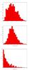 |
Fig. 1 From top to bottom: redshift, mass, and richness distributions for the halos in the sample. Richness refers to cluster galaxies brighter than H∗(zp) + 1.5 and within r200 radius of each halo. |
Concerning redshifts z ≳ 2 we also consider our results cautiously. This is mainly because the properties of galaxy clusters and groups are highly uncertain at these redshifts (Toshikawa et al. 2014; Kubo et al. 2015; Diener et al. 2015; Muldrew et al. 2015), where forming galaxy (proto)clusters are expected to be associated with a significant fraction of the most massive halos.
4. Method
In this section we introduce a new method to perform robust membership assignments on the basis mainly of photometric redshift information.
We have been inspired by the work of Rykoff et al. (2012) and by their subsequent studies (Rykoff et al. 2014; Rozo et al. 2015) as well as by George et al. (2011). We adopt a similar probabilistic Bayesian formalism to assign membership probabilities. However, through the use of Bayesian inference, we attempt an effective generalization of their work. We use in our method the available information about halos and galaxies within the cluster virial radius: cluster redshifts and cluster center coordinates, as well as coordinates, magnitudes, and photometric redshifts of galaxies.
As discussed below we adopt an operative (almost non-parametric) approach based on galaxy number counts which are estimated locally in the cluster field at given redshift and magnitude bins. This strategy is preferred to that which assumes the a priori knowledge of specific models such as those describing the galaxy luminosity function and cluster radial profiles. Our choice is mainly motivated by our ignorance of the cluster galaxy luminosity function and the cluster radial profiles over the broad range of halo masses considered, especially at redshifts z ≳ 1, where strong evolution of both megaparsec-scale structures and cluster galaxies occurs. Furthermore, assuming a specific cluster profile could lead to a bias if clusters with relaxed and disturbed morphology are not considered separately.
4.1. Catalogs of galaxies and halos
We stress that the method proposed in this paper is not a method to detect clusters of galaxies but a method to assign robust group and cluster membership to galaxies. In full generality we consider a magnitude limited catalog of galaxies (each of them is denoted with the letter g) and a catalog of detected (or simulated) groups and/or clusters (each of them is denoted with the letter c), similarly to those used in this work.
For each galaxy we consider i) the observed magnitude mg in a given reference band; ii) the right ascension – declination coordinates (RAg, Decg); and iii) the photometric redshift.
Similarly, for each group/cluster we consider i) the right ascension – declination coordinates (RAc, Decc) of the cluster center (i.e., the barycenter, which is estimated from the cluster members in our case); ii) the radius r200 of the cluster or, alternatively, an estimate of the cluster size in physical units; and iii) the probability density function (PDF) associated with the cluster redshift, Pc(z). All three quantities can be estimated and/or are provided in group/cluster catalogs.
4.2. Adopted strategy
The method we introduce is mainly based on photometric redshifts and galaxy number counts. Similarly to other methods that use photometric redshift information (e.g., Eisenhardt et al. 2008; Bellagamba et al. 2011; Castignani et al. 2014a,b, and references therein) to search for or study galaxy clusters and groups, we consider the redshift information and the coordinates in the projected space separately.
Core sizes are typically in the range 0.1–0.4 Mpc for rich clusters (Bahcall1975; Dressler1978; Sarazin1986), while photometric redshift uncertainties of ±0.03(1 + z) correspond to ~1.0, 0.7, and 0.5 × 10² Mpc at redshifts z = 0.5, 1.0, and 2., respectively.
Therefore photometric redshift uncertainties are much larger (by a factor of ~100) than the typical scale of the cores of clusters and groups and are in fact significantly dominant with respect to any other observable uncertainty (e.g., flux uncertainties, projected space coordinate uncertainties).
A detailed distance discrimination based on photometric redshifts is therefore needed. As it will be clarified below this can be achieved to the detriment of a less detailed tessellation of the projected space.
We adopt a treatment of the projected space (i.e., counts in cells/shells) and the photometric redshift information (i.e., counts in redshift bins) similar to that used in the Poisson Probability Method (PPM, Castignani et al. 2014a,b) which was introduced and applied to search for distant galaxy clusters and groups around a specific point in the sky using photometric redshifts of galaxies and galaxy number counts.
Before introducing our method in the following we will focus on the redshift information.
4.2.1. Redshift information
First we carefully consider, for each galaxy g, the PDF Pg(z) which tells the probability that the spectroscopic redshift of the galaxy zs,g is in the range (z;z + δz). In the case of galaxies for which the spectroscopic redshift is known, Pg(z) is reduced to a very narrow distribution centered at the spectroscopic redshift.
Since we are always considering photometric redshifts, zp,g, we rewrite in a compact form the PDF as the conditional probability distribution P(zs,g | zp,g). The Bayes theorem allows us to relate the PDF to the galaxy redshift distribution N(zs) = dN/ dzs and the PDF P(zp,g | zs,g), which is, by construction, equal to a Gaussian  with mean μ = zs,g and sigma σ = σ0(1 + zs,g). It holds:
  (1)where the normalization is fixed requiring that the integral in zs,g is one. We refer to Sheth & Rossi (2010), where the same equation is derived (their Eq. (1)).
An interesting consequence of Eq. (1) is that, even if photometric redshifts are assigned with a prescription which is independent of the magnitude (by construction, in our case of Gaussian photometric redshifts does not depend on magnitude), the actual functional form of P(zs,g | zp,g) is magnitude dependent because of the presence of the redshift distribution N(zs), which is function of the specific magnitude of the galaxy considered.
Furthermore P(zs,g | zp,g) also depends on the local clustering properties. This is because we are particularly interested in those galaxies that are within the cluster virial radius. The dependence on clustering properties is implicitly present in N(zs), which is in fact the local redshift distribution in the cluster field.
Several previous studies developed similar formalism to study in detail the statistical properties of galaxies in redshift surveys (Efstathiou et al. 1988; Sheth et al. 2007; Benjamin et al. 2007; Fu et al. 2008). However in our case we are interested in estimating locally the redshift distribution N(zs). Therefore we prefer not to estimate the redshift distribution using the entire survey, which would lead to a possible underestimation of the number counts in the case of galaxies within the cluster virial radius. On the other hand if we estimated the redshift distribution using local number counts (e.g., counts in cells) we would be highly affected by low number counts and shot noise, especially at the bright end of the galaxy luminosity function.
Motivated by these aspects, in order not to introduce any artificial bias and systematics in the estimate of P(zs,g | zp,g) in terms of its peak and shape we prefer to consider conservatively a constant redshift distribution N(zs). As it is clear from Eq. (1) such a choice relies implicitly on the assumption that N(zs) does not vary dramatically for zs ≈ zp,g or, more precisely, over the support of P(zs,g | zp,g).
Given the arguments outlined above we therefore derive our final expression for Pg(z) as: ![Mathematical equation: \begin{equation} \label{eq:prob2} P_g(z) \propto\frac{1}{\sigma_0(1+z)}\exp \left[-\frac{(z-z_{{\rm p},g})^2}{2\sigma_0^2(1+z)^2}\right], \end{equation}](/articles/aa/full_html/2016/11/aa28009-15/aa28009-15-eq112.png) (2)where the normalization is again fixed requiring that the integration in z is equal to one.
(2)where the normalization is again fixed requiring that the integration in z is equal to one.
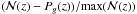
We stress that, while P(zp,g | zs,g) is, by construction, symmetric around zs,g, Pg(zs,g) ≡ P(zs,g | zp,g) is not symmetric around zp,g. In Fig. 2 we show a graphical comparison between P(zs,g | zp,g) and its Gaussian approximation  . When compared to the Gaussian approximation the PDF reported in Eq. (2) shows a shift in redshift of the peak towards lower redshifts and an excess at high redshifts, as also clear from Eq. (2).
The distortion with respect to the Gaussian approximation is in fact due to the ∝σ0(1 + z) scaling of the statistical redshift uncertainties, which are higher at increasing redshifts and imply an increasing spread of the photometric redshift distribution with increasing spectroscopic redshifts.
While the correction is relatively small (i.e., at percent level), we stress that it plays a role in determining membership assignments more accurately, which is particularly important in the context of (future) high-precision cosmological studies. Our findings are also consistent with previous work by Sheth & Rossi (2010), who found discrepancies when comparing statistically the two PDFs, P(zs,g | zp,g) and P(zp,g | zs,g), when drawn from the SDSS survey.
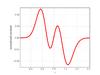 |
Fig. 2 Graphical comparison between Pg(z) as in Eq. (2) and its Gaussian approximation |

In order to apply our formalism to the case of membership assignments, we consider the following prescriptions, concerning the redshift space, as in George et al. (2011). For practical reasons we discretize Pg(z) given in Eq. (2) within the redshift range z = 0−3, which safely includes all redshifts of the halos considered in our sample. We also use consecutive and finite redshift bins δz = 0.01, which assure a good redshift sampling in the case of typical photometric redshift surveys. In order to avoid a spiky behavior of Pg(z) due to the adopted discrete binning we also safely convolve Pg(z) with a Gaussian  which implies a suppression of high-frequency ≳1 /δz fluctuations.
In full analogy with the formalism outlined, for each halo c, we assume Pc(z) to be a Gaussian,  , where zc denotes here some estimate for the cluster redshift. Galaxy clusters are detected from photometric redshift surveys with a typical statistical redshift accuracy σc ≃ σ0/ 2 (Wen et al. 2009, 2012). We nevertheless assume σc = σ0. This represents a conservative choice. Concerning our case of simulated Gaussian photometric redshifts our choice ultimately favors slightly higher values of completeness despite of slightly lower values of purity for our membership assignments. We refer to Sect. 5.1 and Fig. 6 (bottom right panel), where the impact of choosing different values of σc is tested.
Then we discretize Pc(z) and remove high-frequency ≳1 /δz fluctuations applying a Gaussian convolution, analogously to what has been done for Pg(z).
We will always consider zc equal to the value of the halo redshift, estimated in Sect. 3.2. Even if uncertainties could affect the estimates of the cluster redshift as well as of all other cluster properties we point out that we prefer not to include them in this work. This is mainly because one of the main goals of this work is to introduce and test our method against photometric redshift catalogs under controlled statistical uncertainties which are limited to the galaxy catalog. The impact of systematics and uncertainties on the cluster properties will be studied in a following work.
We also stress that the above outlined strategy is tailored to the specific properties of the photometric catalog considered and in particular to the prescription used to assign photometric redshifts. A different strategy could be possibly applied in the case of more realistic photometric redshift catalogs which include more complex statistical as well as systematic uncertainties.
4.2.2. Photometry
Accordingly to the galaxy catalog redefinition performed in Sect. 3.1, in order to perform membership assignments we consider the photometry of the galaxies in H-band, which is the reference band of our catalog. We prefer not to use additional information in other bands such as color information and bivariate galaxy luminosity functions. In fact, since our main goal is to perform membership assignments for galaxies in groups and clusters over a broad range of redshifts and cluster masses we do not want to be biased towards specific galaxy colors, whose distribution and evolution with both redshift and cluster mass are still debated, especially at z ≳ 1.
In full analogy with the strategy adopted for the redshift information, for each galaxy g we define the PDF  which tells the probability that the H-band magnitude of the galaxy is in the range (m;m + δm). We also discretize the problem considering consecutive and discrete bins δm = 0.1 down to H = 26 and conservatively assume
  , where mg is the observed magnitude of the galaxy. The adopted σ if equal to the bin size, which is on the order of the typical statistical photometric uncertainties we expect. Therefore our formalism effectively reproduces the statistical magnitude uncertainties and suppresses high-frequency ≳1 /δm noise in the discrete PDF.
4.2.3. Number densities
Within the framework described in the previous sections we introduce here the mean background number density Nbkg(m,z) which is the mean galaxy number counts per unit redshift, magnitude, and solid angle. The background densities are estimated both globally (i.e., considering a Ω = 10.61 sq. deg rectangular area inscribed in the light cone of the survey) and locally (i.e., considering for each halo the annulus comprised within 3 and 5 Mpc from the halo center). We refer to the two estimates as  and
and  , respectively.
We can define  , where the sum is performed over all galaxies which are within the rectangular area considered. is defined analogously, where the galaxies in each annulus and the associated area are considered. The (discrete) PDFs Pg(z) and Pg(m) satisfy the condition ∑ iPg(zi) = ∑ jPg(mj) = 1, where the summation is performed over bins of redshift (δz) and magnitude (δm) centered at zi and mj, respectively.
Remarkably, the delocalization in redshift through the use of the PDF partially overcomes some problems originated by photometric redshift uncertainties such as the difficulty and ambiguity in determining physical (redshift dependent) distances among sources. In fact the PDF in redshift provides us a general tool to define number counts, as well as to convert the subtended solid angles into physical areas and, therefore, number counts into number densities.
Then we define the following running mean integrating both in redshift and magnitude. This is done to avoid very low number counts which are originated by the small magnitude and redshift bins adopted. It holds:  (3)where σ(z) = σ0(1 + z) denotes the 1σ statistical redshift uncertainty. An analogous definition could be introduced for . However, because of the limited area adopted for the local background selection we may be still affected by small number counts, especially at the bright end of the luminosity function. Therefore, when estimating
  we prefer to adopt the same functional form as in
  , normalizing for the number counts down to H∗(z) + 1.5, as follows:
  (4)where
 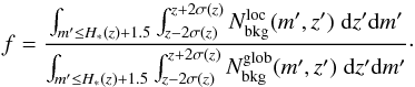 (5)The running means and are crucial quantities for our membership assignments.
In Fig. 3 we plot the distribution of the f-factor for the halos in the sample. The median of the distribution is in 1.09 ± 0.19, consistent with f = 1 within the reported (relatively small) rms dispersion. The fact that the distribution is centered at a value slightly higher than one (the mean value is 1.10) might be explained by the fact that the local background probes scales that are smaller than those of the global background and are therefore characterized by higher clustering.
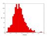 |
Fig. 3 Distribution of the f-factor for the halos in the sample, estimated at the cluster redshift. |
Even if 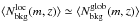 we nevertheless prefer to use (unless otherwise specified) because it better traces the local density around the cluster. It is in fact commonly used when estimating the cluster size from real surveys. Furthermore, in the case of pointed observations of clusters it is the only one which is available.
For each halo c we also introduce the local number density Ntot,c(m,z,r) which is equal to the galaxy number counts per unit redshift, magnitude, and solid angle at a given projected physical separation within (r;r + dr) from the halo center. Here, for each halo we assume azimuthal symmetry around the axis connecting the observer and the halo center. This choice is mainly due to the need of sufficient number statistics that is obtained through the use of counts in cells/shells. Our assumption is also motivated by previous statistical studies, which widely used azimuthal symmetry in determining cluster radial profiles and luminosity functions of cluster galaxies (Biviano et al. 2013). Similarly to what has been done for the background, Ntot,c(m,z,r) is derived using the full PDFs in redshifts and magnitudes, while positional uncertainties are neglected. In analogy with the background, in order to limit shot noise fluctuations, we similarly define a running mean as follows:
 (6)
(6)
where r< and r> are the projected separations which define a subtended area, centered at r, equivalent to that of a circle of 450 kpc radius at redshift z. This size is typical of the core of rich groups and clusters.
We stress again here that, because of the delocalization in redshift of each galaxy through the use of the full PDF, both Ntot,c(m,z,r) and Nbkg(m,z) are well defined quantities.
Using the formalism developed in the present and previous Sections in the following we describe our procedure to assign membership probabilities.
4.3. Membership probability
We consider a specific cluster/group c and a galaxy g in its field and we ask which is the probability  that the galaxy g belongs to the cluster c, i.e., g ∈ c.
All information outlined in the previous sections, useful when assigning membership, is summarized in a more compact form as:  (7)where rc,g(z) is the projected physical distance between the cluster center and the galaxy coordinates. The pedices g and c simply denote that we are referring to the galaxy g and the halo c, respectively.
The spirit behind this work is to assign membership using a distance discrimination based on photometric redshifts (see also Sect. 4.2). Therefore, we use Bayesian inference and express the membership probability putting emphasis on the redshift information as follows: 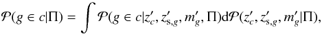 (8)where
  is the conditional probability of the event A given B. The posterior probability distribution in the integrand is simply3 d
 , where we consider independently the magnitude information of the galaxies, as well as the redshift information for both the galaxy and the cluster, i.e.,
  .
.
We estimate  , i.e., the probability that the galaxy belongs to the cluster knowing the redshift
  of the cluster, the spectroscopic redshift (
 ), and the magnitude (
 ) of the galaxy, as well as all information in Π. Such a probability is given by the following number count excess:
 ![Mathematical equation: \begin{equation} \label{eq:pmem2} \mathcal{P}(g\in c| z'_{c},z'_{{\rm s},g},\Pi) = \left[1- \frac{N_{{\rm bkg},c}^{\rm loc}(m'_g,z'_{c})}{N_{{\rm tot},c}(m'_g,z'_{c},r_{c,g})}\right]\phi(z'_{c},z'_{{\rm s},g}), \end{equation}](/articles/aa/full_html/2016/11/aa28009-15/aa28009-15-eq177.png) (9)where
(9)where  is a general non-negative function which is positive and less or equal to one for
  . Here δz(c,g) is a generic function of cluster and/or galaxy properties. Its value is determined by the velocity dispersion of galaxies in the cluster, i.e., ≲2000 km s-1, equivalently δz(c,g) ≲ 0.007(1 + zc) (Evrard et al. 2008). As mentioned in Sect. 2.2 such a dispersion is however much smaller than typical photometric redshift uncertainties. The function thus approximately reduces in our case to a delta Kronecker
  , which is equal to one whenever both and belong to the same redshift bin of width δz. Under the framework outlined above we provide the following expression for the membership probability:
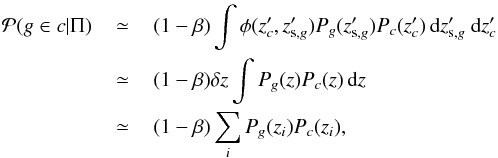
![Mathematical equation: \begin{eqnarray} \label{eq:pmem5} &&\mathcal{P}(g\in c|\Pi) = \int\left[1- \frac{N_{{\rm bkg},c}^{\rm loc}(m'_g,z'_{c})}{N_{{\rm tot},c}(m'_g,z'_{c},r_{c,g})}\right]\nonumber \\&&\qquad \qquad\qquad\times\phi(z'_{c},z'_{{\rm s},g}){\rm d}\mathcal{P}(z'_{c},z'_{{\rm s},g},m'_g|\Pi). \end{eqnarray}](/articles/aa/full_html/2016/11/aa28009-15/aa28009-15-eq185.png) (10)
(10)
The equation suggests that the membership probability can be also interpreted as the averaged number count excess, where the average is performed with the posterior probability distribution as probability measure.
As mentioned in Sect. 4.2.3 small number counts affect number densities which motivate us to factorize the number count excess out of the integral and approximate the membership probability as follows:
 (11)
(11)
where the last expression explicitly shows the discretization in redshift adopted in the formalism. The Kronecker delta approximation of φ is also exploited. The term: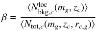 (12)is such that 1−β is the number count excess that is factorized out of the integral of Eq. (10) and is assumed equal to a constant value. Such a value is estimated through the use of average number counts evaluated at the cluster redshift zc and the magnitude mg of the galaxy. The local number density Ntot,c is also evaluated at the projected separation rc,g of the galaxy from the cluster center, as in Eq. (6).
Furthermore, number counts are averaged in radius (r< ≤ r ≤ r>), magnitude ( ), and redshift (
 ), consistently with the above definitions for
  and ⟨ Ntot,c ⟩. Such a filtering allows us also to mitigate possible statistical uncertainties such as those on cluster center coordinates, on photometry, and on photometric redshift over scales smaller than those associated with the average procedure.
The probability is set to zero in those cases where  . Excluding these cases and limiting ourselves to true halo members the median and mean number count excess 1-β, and the rms dispersion around the median are 0.72, 0.68, and 0.19, respectively.
Through the use of Eq. (10) we operatively take into account in our formalism i) the magnitude distribution of field galaxies; ii) the magnitude distribution of cluster galaxies; and iii) the radial distribution of galaxies in clusters. The three points are exploited through the use of number counts at different bins in magnitude and distance to the cluster center and without assuming specific models for the luminosity function and the cluster profile. Nevertheless, membership probabilities could be used to estimate a posteriori both the luminosity function of cluster galaxies and the cluster profile (see e.g., Dahlén et al. 2002, 2004).
Although the main goal of this paper is to introduce our method and test it with simulations we point out that Eq. (10) is a fully general formula for the membership probability that can be applied to any list of clusters and photometric redshift catalog of galaxies. Any systematic or statistical uncertainty as well as additional information such as redshift bias, spectroscopic redshifts, and positional uncertainties can be incorporated in our Bayesian formalism through the use of additional posterior distributions.
4.3.1. From relative to absolute probabilities
The membership probabilities reported in Eqs. (10) and (11) are relative probabilities in the sense that they refer to the chance a galaxy has of occupying an optimal (and relatively small) region in the space of parameters that fiducial cluster members are associated with. In our case the adopted parameters are the redshifts, the cluster centric distance, and the H-band magnitude of galaxies. For example a galaxy in the cluster core with a photometric redshift close to that of the cluster will be associated with higher probability than a galaxy located at a different redshift and at the periphery of the cluster.
To illustrate better the concept we analytically compute the membership probability under the approximation that the PDFs Pc(z) and Pg(z) are both Gaussian functions, which is a few-percent precision approximation (see also Fig. 2). It holds:
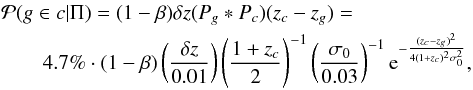 (13)
(13)
here Pg ∗ Pc denotes the convolution between the functions Pg and Pc.
Our result implies that membership probabilities on the order of percent are expected for the cluster members. This is not surprising: given the high photometric redshift uncertainties associated with galaxies (~few 10 Mpc), if compared to the cluster physical size (~1 Mpc), the probability that both the cluster and a cluster member are located at the same distance from the observer along the line of sight is just on the order of ~1% at maximum. Furthermore the maximum probabilities are reached in the limiting case of negligible background or, equivalently, when the cluster is extremely rich (i.e., β ≪ 1).
We note that, consistently with our definition, increasing the number of relevant parameters will increase the dimensionality of the parameter space thus reducing probabilities.
The membership probabilities are also not completely model independent quantities since they scale with the redshift bin δz. However, this dependence simply introduces the scaling  and can be neglected as far as σ0(1 + zc) >δz ≫ δz(g,c), at it is in our case.
Our membership probabilities scale also linearly with the number count excess (1−β), similarly to previous work by Rozo et al. (2009), and show a self-similar Gaussian decay in redshift, at least under the pure Gaussian approximation. Our estimate also shows a clear dependence on the cluster redshift as well as on the statistical photometric redshift accuracy of the considered catalog. In fact, since photometric redshift uncertainties increase with increasing redshift, the maximum achievable probability decreases with increasing redshift, as expressed by the 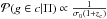 scaling in Eq. (13).
All these scaling relations inspired us to translate our relative probabilities into absolute membership probabilities Pmem assuming self-similarity among clusters at different redshifts: we require that in the limit of negligible background or, equivalently, when the cluster is extremely rich (i.e., β ≪ 1) the maximum membership probability achievable is exactly one, independently of the cluster redshift. In fact, in the limit where β ≪ 1 almost all galaxies within the cluster radius and around the cluster redshift are cluster members.
An effective way to exploit such a limit is to rescale the relative probability with respect to its maximum as follows: 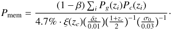 (14)This is our final expression for the membership probability we will use throughout this work. The numerator of the equation is equal to the relative probability
  and the denominator is its maximum value, which is reached at the limit of β ≪ 1, as in Eq. (13). The function ξ(zc) is the correction needed when the Gaussian approximation of Pg(z) is relaxed. We estimate the function ξ numerically.
In Fig. 4 we report 1−ξ as a function of redshift. Such a correction is limited to a few percent and increases with decreasing redshifts down to z = 0.09 below which the support of the Gaussian PDF (σ0 = 0.03 is assumed) is significantly truncated at z = 0. This truncation implies that 1−ξ decreases at lower redshifts (z< 0.09) with decreasing redshift.
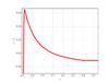 |
Fig. 4 Correction 1−ξ as a function of redshift, see Eq. (14). The correction is up to 4.3% percent at maximum. Galaxies with a photometric redshift accuracy σ0 = 0.03 are considered. |
5. Results: testing the membership assignments
In this section we present our results and quantify their robustness in terms of completeness and purity of our membership assignments.
For each cluster Nestimated is the number of galaxies that are considered cluster members according to the membership assignments, Ntrue is the number of true cluster members, Ninterlopers is the number of sources that are erroneously considered cluster members according to the membership assignments, and Nmissed is the number of true cluster members that are not selected. The four number counts are related as follows: Ntrue = Nestimated + Nmissed−Ninterlopers.
Such numbers are always estimated within the r200 radius, unless a radial interval is specified. Furthermore, when neither a radial nor a magnitude range is specified, the number Ntrue refers to the cluster richness or, equivalently, to the halo occupation number, which is the number of galaxies brighter than a given limit (H∗ + 1.5 in this work) contained in a halo of a given mass (Peacock & Smith 2000).
Following the notation reported in George et al. (2011) we define purity p and completeness c of our assignments as:
Purity and completeness are related according to the following relation: 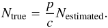 (17)Such a relation is a powerful tool to estimate the true richness of the cluster (Ntrue), once the number of selected cluster members (Nestimated) and the ratio p/c of our assignments are known.
5.1. Completeness vs. purity diagrams
A practical way to select the fiducial cluster members on the basis of our membership assignments is to consider as cluster members all Nestimated galaxies that are associated with membership probabilities Pmem higher than a given threshold Pthr (similarly to George et al. 2011), so that both purity and completeness can be parametrized by Pthr. Such a prescription implies that the robustness of our assignments can be evaluated in terms of the Receiver Operating Characteristic (ROC, Metz 1988).
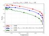 |
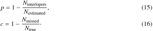
Fig. 5 Purity vs. completeness mean values for the membership assignments. For each cluster galaxies brighter than H∗(zp) + 1.5 and with a projected distance from the cluster center not greater than r200 are considered. Different colors refer to different statistical redshift accuracy σ(z) = σ0(1 + z). Dots show the mean values of both completeness and purity for galaxies with Pmem>Pthr, as indicated in the label. Pthr increases from the right to the left. The errors in the mean values are within the dot size. |
In Fig. 5 we show the ROC curve associated with our assignments where all halos in our sample are considered. Mean values of both completeness and purity are plotted as a function of Pthr. The uncertainties in the mean values are at sub-percent level and therefore negligible. Concerning the photometric redshift catalog with σ0 = 0.03 the mean values of purity and completeness are  and
and  , respectively. The different values refer to increasing Pthr = 10,20,30,50,70, and 80%, respectively. The corresponding median values are
  ,
,  ,
,  ,
,  ,
,  ,
,  and
and  ,
,  ,
,  ,
,  ,
,  ,
,  , where the uncertainties refer to the 68% quartiles.
We then fix a threshold Pthr = 20%, which allows us to have good mean values of both purity and completeness ( and
and  ), as well as a limited associated 68% dispersion (
 and
and  ), which ultimately reflects into reliable richness estimates, see also Eq. (17) and Sect. 6.
Because of the non-negligible 68% scatter, our membership assignments should be considered cautiously if used for single cluster studies. However given the good values of the mean for both purity and completeness as well as the negligible uncertainty in the mean we argue that the assignments are statistically robust, when large samples of clusters are considered.
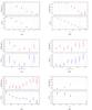 |
Fig. 6 Mean completeness and purity along with associated errors as a function of galaxy magnitude (panel a)), projected separation, in r200 units, of the galaxy from the cluster center (panel b)), halo mass (panel c)) and richness (panel d)), cluster redshift (panel e)), and cluster redshift accuracy σc/σ0 (panel f)). Richness refers to cluster galaxies brighter than H∗(zp) + 1.5 and within r200 radius of each halo. All values refer to σ0 = 0.03 and a probability threshold Pthr = 20%. |
In Fig. 6 we show, for fixed Pthr = 20%, the dependence of both completeness and purity on galaxy magnitude, separation of the galaxy from the cluster center, halo mass and richness, cluster redshift, and cluster redshift accuracy σc.
We observe remarkably stable mean values for both purity and completeness, with variations on the order of a few percent when the dependence on halo mass, richness, and cluster redshift accuracy are considered. A strong decline, in particular for purity is observed when faint ~0.25 L∗ sources (Δp ≃ 30%), and those at the outskirts of the halos (Δp ≃ 50%, at cluster-centric projected distances ~r200) are considered, for which the contamination of field galaxies is significant. Similarly a Δp ≃ 20% decline in purity is observed within the redshift range z ~ 0−2.
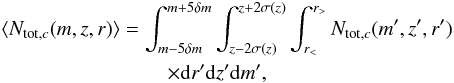
5.2. Membership probability distribution
In Fig. 7 we show the distribution of the membership probabilities for all galaxies in the fields of the clusters in our sample, i.e., with a cluster-centric projected distance not greater than r200. The median values of Pmem for the galaxies with Pmem>Pthr = 10,20,30,50,70, and 80% are Pmem, median = 0.51 ± 0.21,0.55 ± 0.18,0.58 ± 0.15,0.66 ± 0.10,0.77 ± 0.06, and 0.84 ± 0.04, respectively. The reported uncertainty is the rms dispersion. These median values are consistent within a few percent with the corresponding mean values of purity  reported above, respectively, with the only exception represented by the last value associated with Pmem>Pthr = 80%, for which marginal agreement is found.
The fact that the median values of Pmem are both higher than the corresponding Pthr and consistent with the associated  ultimately explains the apparent discrepancy between and the corresponding Pthr in the completeness vs. purity curve of Fig. 5.
Furthermore, the distribution of Fig. 7 has a minimum around Pmem ≈ 20%. The presence of such a minimum is mainly due to the contamination of field galaxies associated with relatively low membership probabilities. The presence of the minimum is also due to the absence of faint galaxies with H>H∗(z) + 1.5 and galaxies with a cluster-centric projected distance higher than the cluster radius, which are in fact not considered. They would nevertheless be associated with low values of 1−β, thus populating the low-probability tail of the Pmem distribution.
The location of the minimum at Pmem ≈ 20% also strengthens the choice of Pthr = 20% as fiducial threshold (as for example in Fig. 6), limiting the contamination of field galaxies. Furthermore, as mentioned above, galaxies with Pmem>Pthr = 20% have Pmem,median = 0.55 ± 0.18, which is consistent, within the dispersion, with analogous Pmem> 50% cut adopted by previous work (George et al. 2011).
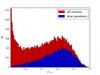 |
Fig. 7 Red: distribution of membership probabilities for the galaxies with Pmem> 20%, brighter than H∗(zp) + 1.5, and with a projected distance from the cluster center not greater than r200. Galaxies with Pmem> 2% are considered to avoid field galaxies associated with small membership probabilities. Blue: same distribution but for the subsample of true cluster members. |
5.3. Fraction of true members
In this section we further test the robustness of our membership assignments. In Fig. 8 we plot the fraction of true members (ftrue) for galaxies belonging to different bins of Pmem. We also consider four different redshift ranges. An overall agreement between Pmem and ftrue is found, independently of the photometric redshift accuracy σ0, within a few-percent precision, as reported in the figure.
Figure 8 shows a flattening of ftrue with increasing redshift for values Pmem ≳ 60%, where the membership probabilities are biased high, although at these Pmem values ftrue is endowed with large uncertainty due to small number counts.
We investigate statistically the goodness of our assignments evaluating the consistency of the ftrue vs. Pmem scatter plot with respect to the one-to-one line by means of χ2 statistics (similarly to Rozo et al. 2015, see their Eqs. (36) and (37)). Concerning the fraction ftrue, Poisson number count uncertainty is added in quadrature to a fiducial (relatively small) error δftrue = 3%.
The δftrue correction is on the order of ftrue vs. Pmem offset and scatter reported in Fig. 8 and outlined in the following. The correction is effective in absorbing the Pmem uncertainties and is ultimately needed to obtain reasonable reduced chi-square values  (see e.g., Bourdin et al. 2015; Castignani & De Zotti 2015, for a similar approach in a different context).
In Table 1 we summarize our results for different redshift bins. A few-percent ftrue vs. Pmem offset, i.e., ⟨ ftrue−Pmem ⟩ < 0, also shown in Fig. 8, is found. It is mainly due to the above mentioned flattening of ftrue for high values of Pmem. In the following we further reconsider the scatter plot to understand the origin of the few-percent ftrue vs. Pmem discrepancy.
Membership results for rescaled probabilities Pmem.
Faint and bright galaxies with magnitudes higher and lower than H∗(z) have ⟨ ftrue−Pmem ⟩ = (−2.9 ± 3.3)% and (− 4.9 ± 8.8)%, respectively. Similarly, rich and poor clusters with more and less than 25 members have ⟨ ftrue−Pmem ⟩ = (−0.8 ± 3.3)% and (−5.7 ± 7.9)%, respectively. The reported values agree with each other within the uncertainties at a few-percent level.
On the other hand a significant discrepancy of a few 10% occurs when galaxies within and beyond r200/ 2 are considered separately. Mean values ⟨ ftrue−Pmem ⟩ = (+11 ± 13)% and (−28 ± 20)% are in fact found, respectively.
In Fig. 9 we show the scatter plot in the two cases and in the case where no radial cut is applied. In the last case an overall agreement with respect to the one-to-one line is found ⟨ ftrue−Pmem ⟩ = (−4.1 ± 5.6)%, although a few-percent ftrue vs. Pmem discrepancy is still detected, on average. In the figure, at variance with what has been done before, all galaxies and halos in the sample are altogether considered without dividing them in redshift bins.
We conclude that the discrepancy is originated neither by faint galaxies nor by poor clusters, but it is mainly due to the contamination of field galaxies at the outskirts of the clusters. Such results are consistent with a significant few 10% decrease Δp in purity with increasing cluster-centric projected distance reported in Fig. 6, also found in previous work (George et al. 2011). Nevertheless, we stress that our sample is mainly constituted by small clusters and rich groups, for which an accurate consideration of the cluster profile is challenging. Such a difficulty could be overcome considering more massive clusters (work in prep.), where the contamination from field galaxies is less significant and/or including in our formalism the cluster radial profile (when known with sufficient accuracy) as additional prior information. In fact we checked that when we limit ourselves to the subsample of 27 clusters with a richness Ntrue ≥ 40 our results significantly improve (χ2/ d.o.f. = 2.92/10 and ⟨ ftrue−Pmem ⟩ = (1.7 ± 2.0)%), which is consistent with the increase Δp ≳ 10% in purity and a few-percent increase in completeness with increasing richness, reported in Fig. 6 within the richness range spanned by our sample.
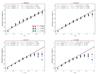 |
Fig. 8 Fraction of true cluster members (ftrue, y-axis) for galaxies brighter than H∗(zp) + 1.5 which membership probabilities (Pmem) reported in the x-axis are assigned to. Points are associated with at least five sources per bins. See Legend in the top left panel for the color code adopted. Different colors refer to different statistical redshift accuracy σ(z) = σ0(1 + z). Mean values and Poisson uncertainties added in quadrature to δftrue = 3% are reported. Upper limits are at 2σ level. Different panels refer to different redshift intervals. At the top of each panel the reduced χ2, the mean difference ⟨ ftrue−Pmem ⟩, and the rms dispersion around the mean are reported. Upper limits are considered as true measurements when estimating ⟨ ftrue−Pmem ⟩. |
5.4. Correlated structures
In this section we examine how the presence of correlated structures affects our results. First we exploit our simulations rejecting from both local and global background areas, when estimating the background, all sources belonging to halos with masses ≥1013M⊙. This has the net effect of increasing Pmem, thus increasing also both the average bias ⟨ ftrue−Pmem ⟩ = (−6.6 ± 4.6)% and χ2/ d.o.f. = 47.4/10 with respect to the case where no correlated structure is removed and all halos in the sample are considered.
When galaxies belonging to halos more massive than 1013M⊙ are rejected also from the cluster field, i.e., a projected distance from the cluster center not greater than r200 is considered, the average bias disappears (⟨ ftrue−Pmem ⟩ = (−0.87 ± 9.1)%). However both the scatter (9.1%) and associated χ2/ d.o.f. = 47.8/10 are higher than the values 5.6% and χ2/ d.o.f. = 4.5/10, respectively, obtained in the case where no correlated structure is removed (see Sect. 5.3). This is ultimately due to the fact that when correlated structures are removed from the cluster field number counts are reduced and higher shot-noise fluctuations affect the results implying the observed higher scatter and higher reduced chi-square values.
Therefore, we find that correlated structures affect the observed Pmem vs. ftrue offset similarly (but less dramatically) to field galaxies at the outskirts of the cluster (see Sect. 5.3). Our results also suggest that correlated structures have to be removed both in the cluster field and in the background areas to reduce the Pmem bias. Nevertheless this approach is critical and does not ultimately improve the results in terms of Pmem vs. ftrue scatter, on average, in our case of low-number statistics and relatively poor clusters.
Interestingly, similarly to our results, Rozo et al. (2015) found that their membership probabilities are biased high when correlated structures are not removed (see also Rykoff et al. 2012, 2014). They corrected the probabilities for the presence of correlated structures, assuming that the number of galaxies belonging to them is a constant fraction of the cluster richness. We stress nevertheless that their sample is mainly constituted by rich clusters, at variance with our sample, for which low-number statistics is affecting more the number counts. Therefore, we prefer not to apply any correction, which implies that we avoid specific assumptions on the properties of correlated structures, in agreement with our non-parametric formalism.
5.5. Comparison with previous work
In this section we mainly focus on the comparison of our results with those of George et al. (2011), who used photometric redshift information to address membership for clusters up to z = 1 and halo masses Mhalo ≲ 1014M⊙. They use both real photometric redshifts and simulated galaxy mock catalogs with Gaussian photometric redshifts. The latter case is analogous to ours.
As further outlined in the following our results are globally consistent with those of George et al. (2011) even if better completeness and slightly better purity seem to be achieved in our work. We stress that a strict comparison with previous work is nevertheless impossible mainly because of the different dataset used (e.g., different photometric redshift uncertainties are considered) and the different range of halo masses and redshifts considered.
Limiting ourselves to the 2 sq. deg COSMOS survey (Scoville 2008) and real photometric redshifts the purity reported in George et al. (2011) tends to saturate at high membership probabilities to values ~80% that are similar to ours for σ0 = 0.02 (see their Fig. 4). This occurs despite the small photometric redshift accuracy σ(z) = (0.01−0.02)(1 + z) of the COSMOS survey (Ilbert et al. 2009).
Considering simulated galaxy mock catalogs and in particular that with associated simulated Gaussian photometric redshifts with an accuracy σ0 = 0.05, they report values  and
and  (their Fig. 7). Conversely, as shown in Fig. 5 for σ0 = 0.05, we have
  (
( ) and
) and  (
( ) for Pthr = 20%4. Therefore similar purity values are found and significantly higher completeness (Δc ≳ 20%) is remarkably found in our case.
Moreover we checked that when we limit ourselves to the redshift range z = 0−1, as in George et al. (2011), the purity improves, Δp ≃ 5%, strengthening our results.
As it will be clarified in the following Section, we suggest that the differences with respect to previous studies might be due to a different consideration of the photometric redshift information when estimating the membership probabilities.
5.6. Reconsidering the Pmem rescaling
As described in Sect. 4.3.1 the relative membership probabilities are rescaled assuming self-similarity among clusters at different redshifts to obtain absolute probabilities, which reflect the actual values of purity reported in Sects. 5.1 and 5.3, see also Fig. 8.
An alternative approach would be to define directly the membership probability in such a way that the associated values are close to one for fiducial cluster members, without the need of rescaling. This is a strategy which is commonly adopted in previous work (Brunner & Lubin 2000; George et al. 2011; Rozo et al. 2015). Two possible approaches are exploited in the following.
5.6.1. Kernel φ
We test, within our formalism, the impact of enlarging the support of the function  , which is assumed to be a Kronecker delta, see Eqs. ((10), (11)). A support with a width
  is here adopted for φ. Enlarging the support of φ has the net effect of boosting the membership probabilities towards higher values for galaxies at redshifts close to that of the cluster. This approach is similar to that adopted in previous analyses (Brunner & Lubin 2000; Rozo et al. 2015).
Two different φ functions are tested here: a top-hat kernel  and a Gaussian kernel
 ![Mathematical equation: \hbox{$\phi_{\rm Gauss}(z_c',z_{{\rm s},g}')={\rm e}^{-\frac{(z_c'-z_{{\rm s},g}')^2}{2[\sigma_0(1+z_c)]^2}}$}](/articles/aa/full_html/2016/11/aa28009-15/aa28009-15-eq340.png) .
.
When all clusters in the sample are considered, if φtop−hat and φGauss are separately adopted we obtain, on average,  (χ2/ d.o.f. = 15.1/9 = 1.7) and
  (χ2/ d.o.f. = 166/6 = 27.7), respectively, as opposed to ⟨ ftrue−Pmem ⟩ = (−4.1 ± 5.6)% (χ2/ d.o.f. = 24.5/10 = 2.5), which is found in the case of rescaled membership probabilities (see Fig. 9a).
Biased low membership probabilities are found when the Gaussian kernel φGauss is used, which in fact gives less weight to the wings than φtop−hat, within the 2σ(z) support.
Results comparable to those obtained using rescaled probabilities are obtained when the top-hat filter φtop−hat is adopted. A careful comparison of the results associated with the two cases when redshift bins are considered is reported in Table 2 and shows that rescaled probabilities Pmem implies globally smaller  values and are therefore preferred.
We also mention that in the case of rescaled probabilities we reach Pmem ≳ 90% and similar ftrue values, although endowed with uncertainties. On the contrary, when φtop−hat and φGauss are assumed, probabilities are 55.7% and 83.4% at maximum, respectively.
Our analysis also shows that, when no rescaling is applied, the results are strongly sensitive to the specific functional form of the kernel φ (here φtop−hat and φGauss are considered). Other, rather subjective, choices of the kernel would lead to different results. This last aspect strengthens our choice of φ, which is Kronecker delta, and the a posteriori rescaling of the probabilities which exploits self-similarity.
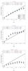 |
Fig. 9 Fraction of true cluster members vs. Pmem, as in Fig. 8, for all halos in the sample. Panel a) refers to galaxies within r200. Panels b) and c) refer to galaxies within and outside r200/ 2, respectively. Color code is the same for all panels. |
Membership results (Cols. 1–3) when the top-hat kernel φtop−hat is adopted.
In the next section we exploit a second independent approach to obtain absolute probabilities without any rescaling.
5.6.2. PDF(z) of galaxies in the cluster field
Our formalism makes use of the full PDF(z) of each galaxy, as reported in Eq. (2). We revisit the expression for the PDF evaluating Pg(zs,g | zc), which is needed in Eq. (8). We write:  (18)which is a convex linear combination of a Dirac delta centered at the cluster redshift and the PDF Pg(zs,g) of Eq. (2). This approach is similar to that adopted in previous studies (George et al. 2011; Rozo et al. 2015).
The convex linear combination is such that, in the presence of a poor cluster, i.e., β ≲ 1, the PDF of the galaxy is close to that of Eq. (2). On the contrary, in the presence of rich clusters, i.e., β ≪ 1, the PDF of the galaxy is centered at the cluster redshift, independently of its photometric redshift.
Therefore the PDF of Eq. (18) operatively takes the clustering of photometric redshifts around the cluster redshift into account. To reject conservatively field galaxies the PDF of Eq. (18) is assigned only to galaxies within a ± 2σ0(1 + zc) interval centered at the cluster redshift zc. Then, we introduce such a PDF in Eq. (11) to obtain a new estimate for the membership probability. Here we adopt the Kronecker delta as φ function. By definition, we note that, independently of the functional form of φ, the membership probability now tends to unity in the limit of rich cluster (β ≪ 1), without any rescaling/modification of the membership probability. We checked that the results (outlined below) do not improve if we consider instead φGauss or φtop−hat.
We observe a significant Δp,Δc ~ 5% decrease of the maximum values achievable for both purity and completeness, with respect to the case where rescaled probabilities are adopted, when averaging among all clusters in our sample. Similarly, we find  and χ2/ d.o.f. = 81/10, when considering all galaxies in the sample. The reduced χ2 is significantly higher than that obtained when rescaled probabilities are adopted (χ2/ d.o.f. = 24.5/10).
We conclude that our rescaled probabilities imply better results concerning both purity and completeness of our assignments with respect to the different tested cases, where i) the PDF(z) of galaxies in the field of clusters (i.e., galaxies with a projected distance from the cluster center not greater than r200) is modified to take operatively the presence of the overdensity into account and/or ii) the support of the function φ is enlarged. In both cases the maximum probabilities achievable have values close to unity, without the need of rescaling.
However for both tested cases the broader range of redshift allowed for the selected cluster members implies higher contamination from non-cluster members (observed in terms of worse purity and higher values) than in the case of our rescaled probabilities, where fiducial cluster members are confined to an optimal region of the space of parameters.
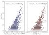 |
Fig. 10 True vs. estimated richness for the 1208 halos in our sample. Richness refers to galaxies brighter than H∗(zp) + 1.5 and within r200 radius of each halo. Galaxies with a statistical photometric redshift accuracy σ0 = 0.03 are considered. Left: richness is estimated as Nestimated, where Pthr = 20% is considered. Right: richness is estimated as the sum of the membership probabilities. The mean logarithmic difference along with the rms dispersion around the mean are reported in the panels. |
5.7. Local vs. global background
We compare our results obtained with a local estimate of the background with those obtained using the global background. Our results do not change, statistically, if the global background estimate is used instead of the local. This is ultimately due to the relatively small dispersion of the f-factor distribution reported in Fig. 3. The results are unchanged even when the tails of the f-factor distribution are considered, as will be clarified in the following.
We consider two subsamples of 30 halos (each of the two corresponds to 2.5% of the entire halo sample) associated with f< 0.7522 and f> 1.537, respectively. We remind that low (high) values of f correspond to low (high) local-to-global background ratios. In the following we show the results for fixed threshold Pthr = 20%.
When f< 0.7522 and the local background are considered the median (mean) completeness and purity are  (
( ) and
) and  (
( ), respectively. When the same threshold f< 0.7522 and the global background are considered the completeness decreases and the purity increases, statistically. The median (mean) values are
  (
( ) and
) and  (
( ), respectively.
When f> 1.537 and the local background are considered the median (mean) completeness and purity are  () and
  (), respectively. When the same threshold f> 1.537 and the global background are considered the completeness increases and the purity decreases, with respect to the case of local background. This corresponds to an opposite behavior with respect to the case when low values of f are considered and it is a consequence of the fact that for low (high) values of f, going from local to global background implies an increase (decrease) of Nbkg and a consequent decrease (increase) of the membership probability. The median (mean) values when the global background is considered and f> 1.537 are in fact
  () and
  (
( ), respectively.
Therefore, overall Δp,Δc ≲ 5% variations in both purity and completeness are observed when considering one background estimate or the other. A significant decrease of the purity Δp ~ 10−20% (nevertheless statistically consistent within the reported 68% uncertainty) is observed when going from low to high values of f. This is expected since the last case corresponds to halos where the local background is intrinsically high.
Interestingly, since f is an observable quantity it could be used in the case of single cluster studies to adjust optimally the threshold Pthr in order to achieve better purity, in particular for clusters with high local background.
6. Results: richness estimates
A remarkable byproduct of our assignments is that we can use them to perform richness estimates (λ). Two richness definitions are considered: i) λ1 = Nestimated (George et al. 2011), which is the number of sources with Pmem>Pthr, where the probability threshold Pthr = 20% is applied, as described above and ii) λ2 = ∑ Pmem (Rozo et al. 2009), where no probability threshold is applied and galaxies are weighted by their membership probability.
6.1. Comparing the two richness estimates
When all halos in the sample are considered (Fig. 10) the mean logarithmic difference between the estimated (λ) and true richness is ⟨ Log(Nestimated/Ntrue) ⟩ = 0.25 ± 0.14 and ⟨ Log( ∑ Pmem/Ntrue) ⟩ = −0.0051 ± 0.15, where the reported uncertainty is the rms dispersion around the mean5. We apply the Spearman test. Evidence of clear correlation between Log(Ntrue) and Log(λ) is found (p-value <1e-150), independently of the richness estimate considered. The values reported in the present and following sections refer to galaxies with a statistical photometric redshift accuracy σ0 = 0.03. However we verified that the richness estimates are remarkably stable when a different photometric redshift accuracy is considered: ⟨ Log( ∑ Pmem/Ntrue) ⟩ = −0.0064 ± 0.14 and −0.0011 ± 0.17, for σ0 = 0.02 and 0.05, respectively.
Our results show that both adopted richness estimates λ lead to similar results, in terms of rms dispersion. When the mean purity and completeness of the assignments are considered, i.e.,  (see Eq. (17)), the mean offset between λ1 = Nestimated and Ntrue disappears, within the rms dispersion. Richness estimates derived as λ2 = ∑ Pmem are instead remarkably unbiased with respect to the true richness Ntrue, on average.
In Tables 3 and 4 we report our results for different redshift and mass intervals, respectively. Our results show that richness estimates are provided with a ~0.10−0.17 dex accuracy, almost independently of the redshift bin considered, within a few 0.01 dex. The lowest dispersion, ~0.07–0.08 dex, is reached for high halo masses, Mhalo ≥ 1014.5M⊙. Therefore, as clarified in the following, our results are fairly independent of the redshift and halo mass intervals considered.
Richness results for different redshift intervals.
Richness results for different halo mass intervals. Column description.
6.2. Richness as mass proxy
We exploit our richness estimates as halo mass proxy. Estimating observable quantities which are tightly correlated with the cluster mass is in fact essential for cosmological studies. First we consider all halos in our sample. The rms dispersion around the mean of the logarithmic difference between the halo mass and the halo occupation number is σ(Log(Mhalo/Ntrue)) = 0.14. Such a scatter is consistent with previous studies (Zheng et al. 2005) and is related to the purely cosmological halo occupation distribution, i.e., the richness distribution for halos of fixed mass. Similarly, when considering our richness estimates we obtain σ(Log(Mhalo/Nestimated)) = 0.20 and σ(Log(Mhalo/ ∑ Pmem)) = 0.20. Our results imply that, to recover the observed halo mass vs. observed richness scatter, an uncertainty of ~0.14 dex, on average, has to be summed in quadrature to the intrinsic σ(Log(Mhalo/Ntrue)) ~ 0.14 scatter, consistently with the relation  .
.
Then we consider different redshift and halo mass intervals, separately (see Tables 3 and 4). The richness vs. halo mass scatter varies within ~0.10–0.21 dex, where the lowest values, 0.10 and 0.14 dex, are reached for halo masses Mhalo ≥ 1014.5M⊙ and redshifts z ≤ 0.75, respectively. These values are remarkably similar to those ~0.1−0.25 found independently using scaling relations based on X-ray and weak lensing studies (Sereno & Ettori 2015), by studies of Sunyaev-Zel’dovich detected clusters (Sereno et al. 2015), as well as by other methods based on galaxy number counts (Andreon 2015). We stress that all these analyses are limited to massive, intermediate/low redshift, and typically relaxed clusters, while our sample is mainly constituted by rich Ntrue ≥ 10 groups spanning a wide range in redshift.
7. Summary and conclusions
7.1. Method
We have introduced a new method to perform statistically robust membership assignments to the galaxies in galaxy clusters using photometric redshift information over an unprecedented broad range of redshift (z ~ 0−2.5) and halo mass (Log(Mhalo) ≃ 13−15), thus extending previous studies (e.g., Brunner & Lubin 2000; George et al. 2011; Rozo et al. 2009).
First relative probabilities are defined (see Sect. 4.3). They correspond to the chance a galaxy has of occupying an optimal region in the parameter space that fiducial cluster members are associated with. The adopted parameters are the redshifts, the cluster centric distance, and the magnitude of the galaxy in a given reference band. Then absolute probabilities Pmem are computed properly rescaling the relative probabilities assuming that in the limit of a very rich cluster Pmem should tend to unity for fiducial cluster members with the highest relative probabilities.
The method takes the magnitude distribution of both cluster and field galaxies as well as the radial distribution of galaxies in clusters into account using a non-parametric formalism (i.e., without assuming specific models) and relies on Bayesian inference to take photometric redshift uncertainties into account. We successfully tested the method against 1208 galaxy clusters with at least ten members brighter than ~0.25 L∗ within r200. The clusters have median redshift z = 1.00 and median mass 1013.87M⊙. They span redshift and mass intervals z = 0.05−2.55 and 1013.29−14.80M⊙, respectively. The clusters are drawn from wide field simulated galaxy mock catalogs mainly developed for the forthcoming Euclid mission (Merson et al. 2013; Gonzalez-Perez et al. 2014). Magnitude limited H< 26 galaxy mock catalogs with different statistical photometric redshift accuracy ~(0.02−0.05)(1 + z) are considered. The catalogs simulate the forthcoming (20.4 sq. deg) Euclid deep survey (Laureijs et al. 2011, 2014).
Membership probabilities are assigned to 22 906 galaxies, 9.8% of them (2236) are considered as true cluster members, which were identified when generating the simulations, according to the halo merging history (Merson et al. 2013).
7.2. Testing membership probabilities
Median purity and completeness values of  and
and  are reached for galaxies brighter than 0.25 L∗ within r200 of each simulated halo and for a statistical photometric redshift accuracy σ((zs−zp)/(1 + zs)) = 0.03. The mean values of purity (
 ) and completeness (
 ) are consistent with the corresponding median values and have negligible sub-percent uncertainties.
We observe stable mean values for both purity and completeness, with variations on the order of a few percent when the dependence on halo mass, richness, and cluster redshift accuracy are considered. The largest departures from the mean values are found for galaxies associated with distant z ≳ 1.5 halos, faint (~0.25 L∗) galaxies, and those at the outskirts of the halo (at cluster-centric projected distances ~r200) for which the purity is lower, Δp ≃ 20% at most, with respect to the mean value.
We have tested the robustness of our membership probabilities Pmem when used as absolute weights by means of the Pmem vs. ftrue scatter plot, where ftrue is the fraction of true members among galaxies with membership probabilities ~Pmem. An overall agreement between the two quantities is found (χ2/ d.o.f. = 24.5/10 = 2.5) at a few-percent accuracy, ⟨ ftrue−Pmem ⟩ = (−4.1 ± 5.6)%.
We suggest that our assignments can be used to estimate weighted cluster radial profiles and cluster galaxies luminosity functions, once the decrease of purity and completeness with radius is taken into account.
We have verified that the few-percent Pmem vs. ftrue discrepancy is mainly due to the contamination of field galaxies at the outskirts (at cluster-centric projected distances ~r200), where the Pmem values are less reliable. Such results are consistent with the above mentioned significant decrease of the purity with increasing cluster-centric distance, also found in previous work (George et al. 2011).
We have exploited the simulations to test the impact of correlated structures with masses ≳1013M⊙. We found that when correlated structures are removed from both the cluster fields, i.e., within the virial radius, and the areas where the background is estimated the Pmem bias disappears (⟨ ftrue−Pmem ⟩ = (−0.87 ± 9.1)%). However both the scatter (9.1%) and associated χ2/ d.o.f. = 47.8/10 are higher than the values obtained in the case where no correlated structure is removed. This is ultimately due to the fact that removing correlated structures implies higher-shot noise, which is critical in our case of low-number statistics and relatively poor clusters.
We also suggest that our results could improve considering more massive clusters (work in prep.), where the contamination from field galaxies is less significant and/or including in the formalism the cluster radial profile (when known with sufficient accuracy) as additional prior information. In particular, we checked that limiting ourselves to the subsample of 27 clusters with true richness ≥40 leads to a significant increase Δp ≳ 10% in purity.
We have tested alternative strategies to define membership probabilities without rescaling. They refer to a different consideration of the redshift information. i) We enlarged the optimal region in the parameter space (concerning the redshift) when defining the relative probabilities using separately a top-hat and a Gaussian kernel, similarly to previous work (Brunner & Lubin 2000; Rozo et al. 2015). ii) We changed the redshift PDF of galaxies in the cluster field, i.e., within the virial radius, to account for the presence of the overdensity of photometric redshifts around the cluster redshift, similarly to previous work (George et al. 2011). In both cases i) and ii) probabilities on the order of unity are reached at maximum for fiducial cluster members, without the need of rescaling. However we verified that our formalism exploiting the rescaling leads statistically to better results than all tested cases.
7.3. Richness estimates
The method is also applied to derive accurate richness estimates. A statistical comparison between the true (Ntrue) vs. estimated (∑ Pmem) richness remarkably yields to unbiased results, Log( ∑ Pmem/Ntrue) = −0.0051 ± 0.15, where the reported values refer to all halos in the sample.
We have also exploited our richness estimates as halo mass proxy. The rms dispersion around the mean of the logarithmic difference between the halo mass and the estimated richness is σ(Log(Mhalo/ ∑ Pmem)) = 0.20. When massive halos ≥1014.5M⊙ are considered the scatter is reduced to 0.10 dex. Our results are fairly consistent with  , where σ(Log(Mhalo/Ntrue)) refers to the (purely cosmological) scatter of the halo occupation distribution.
Our estimates could be useful to constrain the cluster mass function as well as calibrate independent cluster mass estimates such as those obtained from weak lensing, Sunyaev-Zel’dovich, and X-ray studies. Membership assignments derived with our method could be used to perform studies of evolution of galaxies in clusters. Our method can be applied to any list of galaxy clusters or groups in both present and forthcoming surveys such as SDSS, CFHTLS, Pan-STARRS, DES, LSST, and Euclid.
Mock catalog Euclid_v1_LC_DEEP_Gonzalez2014a in the Virgo – Millennium database. Credits: http://galaxy-catalogue.dur.ac.uk:8080/Millennium/Help?page=databases/ euclid_v1/lc_deep_gonzalez2014a
For the sake of clarity the prior Π is omitted in the right-hand side of the expression.
The Pthr = 20% threshold corresponds here (for σ0 = 0.05) to galaxies with a median Pmem = (48 ± 17)%.
We verified that the results only slightly change if the threshold Pthr = 20% is applied also when estimating the richness λ2. In fact in this case we find ⟨ Log [( ∑ Pmem > PthrPmem) /Ntrue] ⟩ = −0.029 ± 0.16.
Acknowledgments
We thank the anonymous referee for very helpful comments. We thank Violeta Gonzalez-Perez, Alex Merson, Carlton Baugh, and Peder Norberg for kindly providing their simulations products which this work is based on and which was created for the Euclid Consortium. We thank them for helpful discussion about their correct use and properties. These simulations products were created on the DiRAC Data Centric system at Durham University, operated by the Institute for Computational Cosmology on behalf of the STFC DiRAC HPC Facility (www.dirac.ac.uk). This equipment was funded by BIS National E-infrastructure capital grant ST/K00042X/1, STFC capital grant ST/H008519/1 and ST/K00087X/1, and STFC DiRAC Operations grant ST/K003267/1 and Durham University. DiRAC is part of the National E-Infrastructure. We thank Chiara Ferrari, Alberto Cappi, Rémi Adam, and Sophie Maurogordato for helpful scientific discussion. We thank Pier-Francesco Rocci, Srivatsan Shridar, and Martin Vannier as well as Guillame Guillon, Alvaro Alonso Rojas Arriagada, and Marina Ricci for helpful discussion about shell scripting and Python coding.
References
- Alberts, S., Pope, A., Brodwin, M., et al. 2013, MNRAS, 1, 2563 [Google Scholar]
- Allen, S. W., Evrard, A. E., & Mantz, A. B. 2011, ARA&A, 49, 409 [NASA ADS] [CrossRef] [Google Scholar]
- Andreon, S. 2015, A&A, 582, A100 [NASA ADS] [CrossRef] [EDP Sciences] [Google Scholar]
- Arnouts, S., Cristiani, S., Moscardini, L., et al. 1999, MNRAS, 310, 540 [NASA ADS] [CrossRef] [Google Scholar]
- Ascaso, B., Mei, S., & Benitez, N. 2015, MNRAS, 453, 2515 [NASA ADS] [CrossRef] [Google Scholar]
- Bahcall, N. A. 1975, ApJ, 198, 249 [NASA ADS] [CrossRef] [Google Scholar]
- Baldry, I. K., Alpaslan, M., Bauer, A. E., et al. 2014, MNRAS, 441, 2440 [NASA ADS] [CrossRef] [Google Scholar]
- Banerji, M., Chapman, S. C., Smail, I., et al. 2011, MNRAS, 418, 1071 [NASA ADS] [CrossRef] [Google Scholar]
- Bassett, R., Papovich, C., Lotz, J. M., et al. 2013, ApJ, 770, 58 [NASA ADS] [CrossRef] [Google Scholar]
- Bellagamba, F., Maturi, M., Hamana, T., et al. 2011, MNRAS, 413, 1145 [NASA ADS] [CrossRef] [Google Scholar]
- Benítez, N. 1999, ASP Conf. Ser., 191, 31 [Google Scholar]
- Benjamin, J., Heymans, C., Semboloni, E., et al. 2007, MNRAS, 820 [Google Scholar]
- Bezanson, R., Wake, D. A., Brammer, G. B., et al. 2016, ApJ, 822, 30 [NASA ADS] [CrossRef] [Google Scholar]
- Birkinshaw, M. 1999, Phys. Rep., 310, 97 [NASA ADS] [CrossRef] [Google Scholar]
- Biviano, A., Rosati, P., Balestra, I., et al. 2013, A&A, 558, A1 [NASA ADS] [CrossRef] [EDP Sciences] [Google Scholar]
- Bocquet, S., Saro, A., Dolag, K., & Mohr, J. J. 2016, MNRAS, 456, 2361 [Google Scholar]
- Bode, P., Bahcall, N. A., Ford, E. B., & Ostriker, J. P., 2001, ApJ, 551, 15 [Google Scholar]
- Böhringer, H., & Werner, N. 2009, A&ARv, [arXiv:0907.4277] [Google Scholar]
- Bolzonella, M., Miralles, J.-M., & Pelló, R., 2000, A&A 363, 476 [Google Scholar]
- Bourdin, H., Mazzotta, P., & Rasia, E., 2015, ApJ, 815, 92 [NASA ADS] [CrossRef] [Google Scholar]
- Brodwin, M., Stanford, S. A., Gonzalez, A. H., et al. 2013, ApJ, 779, 138 [NASA ADS] [CrossRef] [Google Scholar]
- Brunner, R. J., & Lubin, L. M., 2000, AJ, 120, 2851 [NASA ADS] [CrossRef] [Google Scholar]
- Bruzual, G., & Charlot, S., 1993, ApJ, 405, 538 [NASA ADS] [CrossRef] [Google Scholar]
- Campa, J., Flaugher, B., & Estrada, J. 2015, ArXiv e-prints [arXiv:1512.01468] [Google Scholar]
- Casasola, V., Magrini, L., Combes, F., et al. 2013, A&A, 558, A60 [NASA ADS] [CrossRef] [EDP Sciences] [Google Scholar]
- Castignani, G., & De Zotti, G., 2015, A&A, 573, A125 [NASA ADS] [CrossRef] [EDP Sciences] [Google Scholar]
- Castignani, G., Chiaberge, M., Celotti, A., et al. 2014a, ApJ, 792, 113 [NASA ADS] [CrossRef] [Google Scholar]
- Castignani, G., Chiaberge, M., Celotti, A., et al. 2014b, ApJ, 792, 114 [NASA ADS] [CrossRef] [Google Scholar]
- Cavuoti, S., Brescia, M., Tortora, C., et al. 2015, MNRAS, 452, 3100 [NASA ADS] [CrossRef] [Google Scholar]
- Cole, S., Lacey, C. G., Baugh, C. M., & Frenk, C. S. 2000, MNRAS, 319, 168 [NASA ADS] [CrossRef] [Google Scholar]
- Collister, A. A., & Lahav, O. 2004, PASP, 116, 345 [NASA ADS] [CrossRef] [Google Scholar]
- Cui, W., Power, C., Biffi, V., et al. 2016, MNRAS, 456, 2566 [NASA ADS] [CrossRef] [Google Scholar]
- Cunha, C. E., Huterer, D. B., Michael, T., & Wechsler, R. H. 2012, MNRAS, 423, 909 [NASA ADS] [CrossRef] [Google Scholar]
- Dahlén, T., Fransson, C., & Näslund, M. 2002, MNRAS, 330, 167 [NASA ADS] [CrossRef] [Google Scholar]
- Dahlén, T., Fransson, C., Näslund, M., et al. 2004, MNRAS, 350, 253 [NASA ADS] [CrossRef] [Google Scholar]
- Dawson, K. S., Schlegel, D. J., et al. 2013, AJ, 145, 10 [Google Scholar]
- de Propris, R., Eisenhardt, P. R., Stanford, S. A., et al. 1998, ApJ, 503, 45 [Google Scholar]
- The Dark Energy Survey Collaboration 2005, ArXiv e-prints [arXiv:0510346] [Google Scholar]
- Diaferio, A. 1999, MNRAS, 309, 610 [NASA ADS] [CrossRef] [Google Scholar]
- Diaferio, A., Geller, M. J., & Rines, K. J. 2005, ApJ, 628, 97 [Google Scholar]
- Diener, C., Lilly, S. J., Knobel, C., et al. 2013, ApJ, 765, 109 [NASA ADS] [CrossRef] [Google Scholar]
- Diener, C., Lilly, S. J., Ledoux, C., et al. 2015, ApJ, 802, 31 [NASA ADS] [CrossRef] [Google Scholar]
- Dressler, A. 1978, ApJ, 226, 55 [NASA ADS] [CrossRef] [Google Scholar]
- Efstathiou, G., Ellis, R. S., & Peterson, B. A. 1988, MNRAS, 232, 431 [NASA ADS] [CrossRef] [Google Scholar]
- Eisenhardt, P. R. M., Brodwin, M., Gonzalez, A. H., et al. 2008, ApJ, 684, 905 [NASA ADS] [CrossRef] [Google Scholar]
- Ettori, S. 2013, MNRAS, 435, 1265 [NASA ADS] [CrossRef] [Google Scholar]
- Evrard, A. E., Bialek, J., Busha, M., et al. 2008, ApJ, 672, 122 [NASA ADS] [CrossRef] [Google Scholar]
- Fabian, A. C. 2012, ARA&A, 50, 455 [NASA ADS] [CrossRef] [Google Scholar]
- Fioc, M., & Rocca-Volmerange, B. 1997, A&A, 326, 950 [NASA ADS] [Google Scholar]
- Flaugher, B. 2005, Int. J. Mod. Phys. A, 20, 3121 [Google Scholar]
- Fu, L., Semboloni, E., Hoekstra, H., et al. 2008, A&A, 479, 9 [NASA ADS] [CrossRef] [EDP Sciences] [Google Scholar]
- Garilli, B., Guzzo, L., Scodeggio, M., et al. 2014, A&A, 562, A23 [NASA ADS] [CrossRef] [EDP Sciences] [Google Scholar]
- George, M. R., Leauthaud, A., Bundy, K., & Finoguenov, A. 2011, ApJ, 742, 125 [NASA ADS] [CrossRef] [Google Scholar]
- Gifford, D., Miller, C., & Kern, N. 2013, ApJ, 773, 116 [NASA ADS] [CrossRef] [Google Scholar]
- Giodini, S., Lovisari, L., Pointecouteau, E., et al. 2013, Space Sci. Rev., 177, 247 [NASA ADS] [CrossRef] [Google Scholar]
- Gobat, R., Strazzullo, V., Daddi, E., et al. 2013, ApJ, 776, 9 [NASA ADS] [CrossRef] [Google Scholar]
- Gonzalez-Perez, V., Lacey, C. G., Baugh, C. M., et al. 2014, MNRAS, 439, 264 [NASA ADS] [CrossRef] [Google Scholar]
- Guo, Q., White, S., Angulo, R. E., et al. 2013, MNRAS, 428, 1351 [NASA ADS] [CrossRef] [Google Scholar]
- Guzzo, L., Scodeggio, M., Garilli, B., et al. 2014, A&A, 566, A108 [NASA ADS] [CrossRef] [EDP Sciences] [Google Scholar]
- High, F. W., Stalder, B., Song, J., et al. 2010, ApJ, 723, 1736 [NASA ADS] [CrossRef] [Google Scholar]
- Hoekstra, H., Bartelmann, M., Dahle, H., et al. 2013, Space Sci. Rev., 177, 75 [NASA ADS] [CrossRef] [Google Scholar]
- Ilbert, O., Arnouts, S., McCracken, H. J., et al. 2006, A&A, 457, 841 [NASA ADS] [CrossRef] [EDP Sciences] [Google Scholar]
- Ilbert, O., Capak, P., Salvato, M., et al. 2009, ApJ, 690, 1236 [NASA ADS] [CrossRef] [Google Scholar]
- Jiang, L., Helly, J. C., Cole, S., & Frenk, C. S. 2014, MNRAS, 440, 2115 [NASA ADS] [CrossRef] [Google Scholar]
- Jimeno, P., Broadhurst, T., Coupon, J., Umetsu, K., & Lazkoz, R. 2015, MNRAS, 448, 1999 [NASA ADS] [CrossRef] [Google Scholar]
- Kennicutt, Jr. R. C. 1983, ApJ, 272, 54 [NASA ADS] [CrossRef] [EDP Sciences] [Google Scholar]
- Kneib, J.-P., & Natarajan, P. 2011, A&ARv, 19, 47 [NASA ADS] [CrossRef] [Google Scholar]
- Knobel, C., Lilly, S. J., Iovino, A., et al. 2009, ApJ, 697, 1842 [NASA ADS] [CrossRef] [Google Scholar]
- Knobel, C., Lilly, S. J., Carollo, C. M., et al. 2012, ApJ, 755, 48 [NASA ADS] [CrossRef] [Google Scholar]
- Köhlinger, F., Hoekstra, H., & Eriksen, M. 2015, MNRAS, 453, 3107 [NASA ADS] [Google Scholar]
- Komatsu, E., Smith, K. M., Dunkley, J., et al. 2011, ApJS, 192, 18 [NASA ADS] [CrossRef] [Google Scholar]
- Kubo, M., Yamada, T., Ichikawa, T., et al. 2015, ApJ, 799, 38 [NASA ADS] [CrossRef] [Google Scholar]
- Lacey, C. G., Baugh, C. M., Frenk, C. S., et al. 2016, MNRAS, 462, 3854 [NASA ADS] [CrossRef] [Google Scholar]
- Laigle, C., McCracken, H. J., Ilbert, O., et al. 2016, ApJS, 224, 24 [NASA ADS] [CrossRef] [Google Scholar]
- Laureijs, R., Amiaux, J., Arduini, S., et al. 2011 ArXiv e-prints [arXiv:1110.3193] [Google Scholar]
- Laureijs, R., Racca, G., Stagnaro, L., et al. 2014, SPIE, 9143, 91430H [Google Scholar]
- Le Fèvre, O., Tasca, L. A. M., Cassata, P., et al. 2015, A&A, 576, A79 [NASA ADS] [CrossRef] [EDP Sciences] [Google Scholar]
- LSST Science Collaborations and LSST Project 2009, LSST Science Book, ArXiv e-prints [arXiv:0912.0201] [Google Scholar]
- LSST Dark Energy Science Collaboration 2012, ArXiv e-prints [arXiv:1211.0310] [Google Scholar]
- Mamon, G. A., Biviano, A., & Boué, G. 2013, MNRAS, 429, 3079 [NASA ADS] [CrossRef] [Google Scholar]
- Marulli, F., Veropalumbo, A., Moscardini L., Cimatti, A., & Dolag, K. 2016, MNRAS, submitted [arXiv:1505.01170] [Google Scholar]
- Masters, D., Capak, P., Stern, D., et al. 2015, ApJ, 813, 53 [NASA ADS] [CrossRef] [Google Scholar]
- McCracken, H. J., Milvang-Jensen, B., Dunlop, J., et al. 2012, A&A, 544, A156 [NASA ADS] [CrossRef] [EDP Sciences] [Google Scholar]
- McIntosh, D. H., Wagner, C., Cooper, A., et al. 2014, MNRAS, 442, 533 [NASA ADS] [CrossRef] [Google Scholar]
- Mellier, Y. 1999, ARA&A, 37, 127 [NASA ADS] [CrossRef] [Google Scholar]
- Ménard, B., Scranton, R., Schmidt, S., et al. 2013, ArXiv e-prints [arXiv:1303.4722] [Google Scholar]
- Merson, A. I., Baugh, C. M., Helly, J. C., et al. 2013, MNRAS, 429, 556 [NASA ADS] [CrossRef] [Google Scholar]
- Metz, C. E. Basic principles of ROC analysis. Sem Nuc Med., 1978, 8:283 [Google Scholar]
- Mohr, J. J. 2005, in Observing Dark Energy, eds. S. C. Wolf, & T. R. Lauer (San Francisco: ASP), ASP Conf. Ser., 339, 140 [Google Scholar]
- Morandi, A., Ettori, S., & Moscardini, L. 2007, MNRAS, 379, 518 [NASA ADS] [CrossRef] [Google Scholar]
- Muldrew, S. I., Hatch, N. A., & Cooke, E. A. 2015, MNRAS, 452, 2528 [NASA ADS] [CrossRef] [Google Scholar]
- Newman, J. A., Abate, A., Abdalla, F. B., et al. 2015, Astropart. Phys., 63, 81 [NASA ADS] [CrossRef] [Google Scholar]
- Oke, J. B. 1974, ApJS, 27, 21 [NASA ADS] [CrossRef] [Google Scholar]
- Papovich, C., Momcheva, I., Willmer, C. N. A., et al. 2010, ApJ, 716, 1503 [NASA ADS] [CrossRef] [Google Scholar]
- Peacock, J. A., & Smith, R. E., 2000, MNRAS, 318, 1144 [NASA ADS] [CrossRef] [Google Scholar]
- Planck Collaboration XX. 2014, A&A, 571, A20 [NASA ADS] [CrossRef] [EDP Sciences] [Google Scholar]
- Planck Collaboration XXIV. 2016, A&A, 594, A24 [NASA ADS] [CrossRef] [EDP Sciences] [Google Scholar]
- Poggianti, B. M. 2003, Ap&SS, 285, 121 [NASA ADS] [CrossRef] [Google Scholar]
- Rahman, M., Ménard, B., Scranton, R., Schmidt, S. J., & Morrison, C. B. 2015, MNRAS, 447, 3500 [NASA ADS] [CrossRef] [Google Scholar]
- Rahman, M., Ménard, B., & Scranton, R. 2016, MNRAS, 457, 3912 [NASA ADS] [CrossRef] [Google Scholar]
- Ramella, M., Biviano, A., Boschin, W., et al. 2000, A&A, 360, 861 [NASA ADS] [Google Scholar]
- Rosati, P., Borgani, S., & Norman, C. 2002, ARA&A, 40, 539 [NASA ADS] [CrossRef] [Google Scholar]
- Rossetti, M., Gastaldello, F., Ferioli, G., et al. 2016, MNRAS, 457, 4515 [Google Scholar]
- Rozo, E., Rykoff, E. S., Evrard, A., et al. 2009, ApJ, 699, 768 [NASA ADS] [CrossRef] [Google Scholar]
- Rozo, E., Wechsler, R. H., Rykoff, E. S., et al. 2010, ApJ, 708, 645 [NASA ADS] [CrossRef] [Google Scholar]
- Rozo, E., Rykoff, E. S., Becker, M., Reddick, R. M., & Wechsler, R. H. 2015, MNRAS, 453, 38 [NASA ADS] [CrossRef] [Google Scholar]
- Rykoff, E. S., Koester, B. P., Rozo, E., et al. 2012, ApJ, 746, 178 [NASA ADS] [CrossRef] [Google Scholar]
- Rykoff, E. S., Rozo, E., Busha, M. T., et al. 2014, ApJ, 785, 104 [NASA ADS] [CrossRef] [Google Scholar]
- Sadeh, I., Abdalla, F. B., & Lahav, O. 2016, PASP, 128, 968 [Google Scholar]
- Santos, J. S., Altieri, B., Popesso, P., et al. 2013, MNRAS, 433, 1287 [NASA ADS] [CrossRef] [Google Scholar]
- Sarazin, C. L. 1986, Rev. Mod. Phys., 58, 1 [NASA ADS] [CrossRef] [Google Scholar]
- Sarazin, C. L. 1988, Cambridge Astrophysics Series Cambridge: (Cambridge University Press) [Google Scholar]
- Saro, A., Bocquet, S., Rozo, E., et al. 2015, MNRAS, 454, 2305 [NASA ADS] [CrossRef] [Google Scholar]
- Scoville, N. 2008, Ap&SS, 313, 287 [NASA ADS] [CrossRef] [Google Scholar]
- Sereno, M., & Ettori, S. 2015, MNRAS, 450, 3633 [NASA ADS] [CrossRef] [Google Scholar]
- Sereno, M., Ettori, S., & Moscardini, L. 2015, MNRAS, 450, 3649 [NASA ADS] [CrossRef] [Google Scholar]
- Sheth, R. K. 2007, MNRAS, 378, 709 [NASA ADS] [CrossRef] [Google Scholar]
- Sheth, R. K., & Rossi, G. 2010, MNRAS, 403, 2137 [NASA ADS] [CrossRef] [Google Scholar]
- Skelton, R. E., Whitaker, K. E., Momcheva, I. G., et al. 2014, ApJS, 214, 24 [Google Scholar]
- Steidel, C. C., & Shapley, A. E. 2004, ApJ, 604, 534 [NASA ADS] [CrossRef] [Google Scholar]
- Strazzullo, V., Gobat, R., Daddi, E., et al. 2013, ApJ, 772, 118 [NASA ADS] [CrossRef] [Google Scholar]
- Toshikawa, J., Kashikawa, N., Overzier, R., et al. 2014, ApJ, 792, 15 [NASA ADS] [CrossRef] [Google Scholar]
- Wen, Z. L., Han, J. L., & Liu, F. S. 2009, ApJS, 183, 197 [NASA ADS] [CrossRef] [Google Scholar]
- Wen, Z. L., Han, J. L., & Liu, F. S. 2012, ApJS, 199, 34 [NASA ADS] [CrossRef] [Google Scholar]
- White, S. D. M., Efstathiou, G., & Frenk, C. S. 1993, MNRAS, 262, 1023 [NASA ADS] [CrossRef] [Google Scholar]
- York, D. G., Adelman, J., Anderson, J. E., Jr., et al. 2000, AJ, 120, 1579 [Google Scholar]
- Yu, H., Serra, A. L., Diaferio, A., & Baldi, M. 2015, ApJ, 810, 37 [NASA ADS] [CrossRef] [Google Scholar]
- Zeimann, G., Stanford, S. A., Brodwin, M., et al. 2012, ApJ, 756, 115 [NASA ADS] [CrossRef] [EDP Sciences] [Google Scholar]
- Zeimann, G., Stanford, S. A., Brodwin, M., et al. 2013, ApJ, 779, 137 [NASA ADS] [CrossRef] [Google Scholar]
- Zheng, Z., Berlind, A. A., Weinberg, D. H., et al. 2005, ApJ, 633, 791 [NASA ADS] [CrossRef] [Google Scholar]
All Tables
All Figures
|
Fig. 1 From top to bottom: redshift, mass, and richness distributions for the halos in the sample. Richness refers to cluster galaxies brighter than H∗(zp) + 1.5 and within r200 radius of each halo. |
| In the text | |
|
Fig. 2 Graphical comparison between Pg(z) as in Eq. (2) and its Gaussian approximation |
| In the text | |
|
Fig. 3 Distribution of the f-factor for the halos in the sample, estimated at the cluster redshift. |
| In the text | |
|
Fig. 4 Correction 1−ξ as a function of redshift, see Eq. (14). The correction is up to 4.3% percent at maximum. Galaxies with a photometric redshift accuracy σ0 = 0.03 are considered. |
| In the text | |
|
Fig. 5 Purity vs. completeness mean values for the membership assignments. For each cluster galaxies brighter than H∗(zp) + 1.5 and with a projected distance from the cluster center not greater than r200 are considered. Different colors refer to different statistical redshift accuracy σ(z) = σ0(1 + z). Dots show the mean values of both completeness and purity for galaxies with Pmem>Pthr, as indicated in the label. Pthr increases from the right to the left. The errors in the mean values are within the dot size. |
| In the text | |
|
Fig. 6 Mean completeness and purity along with associated errors as a function of galaxy magnitude (panel a)), projected separation, in r200 units, of the galaxy from the cluster center (panel b)), halo mass (panel c)) and richness (panel d)), cluster redshift (panel e)), and cluster redshift accuracy σc/σ0 (panel f)). Richness refers to cluster galaxies brighter than H∗(zp) + 1.5 and within r200 radius of each halo. All values refer to σ0 = 0.03 and a probability threshold Pthr = 20%. |
| In the text | |
|
Fig. 7 Red: distribution of membership probabilities for the galaxies with Pmem> 20%, brighter than H∗(zp) + 1.5, and with a projected distance from the cluster center not greater than r200. Galaxies with Pmem> 2% are considered to avoid field galaxies associated with small membership probabilities. Blue: same distribution but for the subsample of true cluster members. |
| In the text | |
|
Fig. 8 Fraction of true cluster members (ftrue, y-axis) for galaxies brighter than H∗(zp) + 1.5 which membership probabilities (Pmem) reported in the x-axis are assigned to. Points are associated with at least five sources per bins. See Legend in the top left panel for the color code adopted. Different colors refer to different statistical redshift accuracy σ(z) = σ0(1 + z). Mean values and Poisson uncertainties added in quadrature to δftrue = 3% are reported. Upper limits are at 2σ level. Different panels refer to different redshift intervals. At the top of each panel the reduced χ2, the mean difference ⟨ ftrue−Pmem ⟩, and the rms dispersion around the mean are reported. Upper limits are considered as true measurements when estimating ⟨ ftrue−Pmem ⟩. |
| In the text | |
|
Fig. 9 Fraction of true cluster members vs. Pmem, as in Fig. 8, for all halos in the sample. Panel a) refers to galaxies within r200. Panels b) and c) refer to galaxies within and outside r200/ 2, respectively. Color code is the same for all panels. |
| In the text | |
|
Fig. 10 True vs. estimated richness for the 1208 halos in our sample. Richness refers to galaxies brighter than H∗(zp) + 1.5 and within r200 radius of each halo. Galaxies with a statistical photometric redshift accuracy σ0 = 0.03 are considered. Left: richness is estimated as Nestimated, where Pthr = 20% is considered. Right: richness is estimated as the sum of the membership probabilities. The mean logarithmic difference along with the rms dispersion around the mean are reported in the panels. |
| In the text | |
Current usage metrics show cumulative count of Article Views (full-text article views including HTML views, PDF and ePub downloads, according to the available data) and Abstracts Views on Vision4Press platform.
Data correspond to usage on the plateform after 2015. The current usage metrics is available 48-96 hours after online publication and is updated daily on week days.
Initial download of the metrics may take a while.