| Issue |
A&A
Volume 595, November 2016
|
|
|---|---|---|
| Article Number | A71 | |
| Number of page(s) | 16 | |
| Section | The Sun | |
| DOI | https://doi.org/10.1051/0004-6361/201527797 | |
| Published online | 31 October 2016 | |
Variation of the temperature gradient in the solar photosphere with magnetic activity
1 Université Côte d’Azur, Observatoire de la Côte d’Azur, CNRS UMR 7293 J. L. Lagrange Laboratory, Campus Valrose, 06108 Nice, France
e-mail: This email address is being protected from spambots. You need JavaScript enabled to view it.
; This email address is being protected from spambots. You need JavaScript enabled to view it.
2 Indian Institut of Technology Madras, 600024 Chennai, India
Received: 20 November 2015
Accepted: 2 August 2016
Abstract
Context. The contribution of quiet-Sun regions to the solar irradiance variability is currently unclear. Some solar-cycle variations of the quiet-Sun physical structure, such as the temperature gradient or the photospheric radius, might affect the irradiance.
Aims. We intend to investigate possible variations of the photospheric temperature gradient with magnetic activity.
Methods. We used high-resolution center-to-limb observations of the FeI 630.15 nm line profile in the quiet Sun performed onboard the Hinode satellite on 2007, December 19, and on 2013, December 7, that is, close to a minimum and a maximum of magnetic activity, respectively. We analyzed samples of 10″ × 10″ internetwork regions. The wings of the FeI 630.15 nm line were used in a non-standard way to recover images at roughly constant continuum optical depths above the continuum formation level. The image formation height is derived from measuring its perspective shift with respect to the continuum image, both observed away from disk center. The measurement relies on a cross-spectral method that is not limited by the spatial resolution of the SOT telescope and does not rely on any radiative transfer computation. The radiation temperature measured in the images is related to the photospheric temperature at their respective formation height.
Results. The method allows us to investigate the temperature gradient in the low photosphere at altitudes of between 0 and 60 km above the 500 nm continuum formation height. In this layer the internetwork temperature gradient appears steeper in our 2013 sample than in the sample of 2007 in the northern hemisphere, whereas we detect no significant change in the southern hemisphere. We argue that this might be related to some strong hemispheric asymmetry of the magnetic activity at the solar maximum of cycle 24.
Conclusions. Structural changes have been observed in numerical simulations of the magneto-convection at the surface of the Sun where the increase of the ambient sub-surface magnetic fields leads to some steepening of the temperature gradient in the internetwork. Hemispheric asymmetry of the activity has been reported for the last solar cycles with successive dominant north and south hemisphere during the activity maximum. Our results seem consistent with this global physical picture, but need to be confirmed by additional studies.
Key words: techniques: high angular resolution / techniques: spectroscopic / Sun: photosphere / Sun: fundamental parameters
© ESO, 2016
1. Introduction
The variation of the total solar irradiance (TSI) in phase with the solar cycle is now well established thanks to measurements performed from space by dedicated instruments over the past four solar cycles. However, the spectral dependance (SSI) of the solar cycle variability is still a controversial subject (see the reviews by Yeo et al. 2014; Solanki et al. 2013). The direct observation of SSI variations on solar-cycle timescales is a difficult task, and some discrepancies appear, in particular in the UV domain, between different space-based instruments. These variations are an important forcing term for the evolution of the climate on Earth and are related to the understanding of the dynamo processes taking place in the solar interior. The efforts made to model TSI and SSI variations currently rely on the hypothesis that the main drivers of solar variability are magnetic features at the solar surface, and that the thermodynamical state of the quiet-Sun atmosphere is invariant. Semi-empirical models of the different types of features, or components (such as sunspot umbrae and penumbrae, faculae and quiet-Sun network) are used, together with observational records of their surface and location on the solar disk, to reconstruct the SSI variations (see Fontenla et al. 2011).
The frequencies of solar acoustic oscillations also show a well-documented solar-cycle variation (see Fossat et al. 1987; Salabert et al. 2015). The frequency shifts can be interpreted as arising from structural changes in the sub-surface layers, such as changes in temperature (Kuhn et al. 1988) or in the size of the acoustic cavity (Dziembowski & Goode 2005). Changes with the solar cycle of the solar subsurface stratification were inferred by Lefebvre & Kosovichev (2005) from inversion of Solar and Heliospheric Observatory (SoHO) Michelson Doppler Imager (MDI) f-mode frequencies. A variation of the solar radius in antiphase with the solar cycle was derived from these measurements, with a lower limit of 2 km for the peak-to-peak amplitude of the variations. An upper limit of 15 km was inferred by Bush et al. (2010) from one solar-cycle SoHO/MDI observations. Lefebvre et al. (2009) showed that f-mode frequencies are mainly sensitive to the pressure scale height in the sub-surface layers. In a recent paper, Salabert et al. (2015) analyzed eighteen years of measurements of the GOLF experiment onboard SoHO to derive the temporal variability of the frequency shifts of the radial, dipolar, and quadrupolar modes for different frequency ranges sensitive to different layers in the solar sub-surface interior. They showed that the temporal evolution of the magnetic configuration imprints on these modes in a different way during cycle 23 and the weak on-going cycle 24. Moreover, as observed in the sunspot number, the past solar cycles present clear hemispheric asymmetries, with successive dominant north and south hemispheres during the activity maximum.
Recently the analysis of thirteen years of SoHO/VIRGO data by Finsterle et al. (2013) has revealed a slight north-south asymmetry of the solar radiance, which seems to be unrelated to sunspots, faculae, or plages, but instead may be due to some variations of quiet-Sun properties.
A theoretical investigation, based on magnetohydrodynamic (MHD) simulations, of the properties of the granulation in quiet-Sun regions in different magnetic environments was presented in Criscuoli (2013). She showed that an ambient magnetic field gives rise to two main physical effects: it inhibits convection and reduces the average opacity. The two effects have opposite consequences on the temperature gradients: the reducted opacity, which dominates at optical depths close to unity and smaller, reduces the temperature gradient; the inhibited convection, which dominates at optical depths larger than one, steepens the temperature gradient. In internetwork regions, the simulations showed that the temperature in the low photosphere decreases with increasing local magnetic field (see also Criscuoli & Uitenbroek 2014). This study also shows that the temperature decreases in small-scale magnetic structures, such as flux-tubes, when the surrounding magnetic field increases.
Previous observational studies based on differential photometry performed in two continuum bands in the quiet Sun and in magnetic faculae have shown that the temperature gradient is smoother in faculae than in the average quiet Sun (see Foukal et al. 1981; Foukal & Duvall 1985). This is consistent with the results of MHD simulations (Spruit 1976; Deinzer et al. 1984; Riethmüller et al. 2014), it is mainly an effect of the reduced opacity in the magnetic region.
Here we aim at investigating possible structural changes in the quiet-Sun temperature gradient between the last solar minimum and maximum. We focus this study on internetwork regions and consider one set of observations performed at a moment close to the solar minimum on December 19, 2007 and another one close to the last maximum, on December 7, 2013.
We first stress that in 3D atmospheres the mean temperature gradient may be defined in various ways, leading to quite different results (Uitenbroek & Criscuoli 2011; Magic et al. 2013). Here we chose to consider the temperature averaged over layers at constant continuum optical depth because this allows a more meaningful comparison with standard semi-empirical models. The standard way to derive temperatures and temperature gradients is to use photometrically accurate observations in continua formed at different heights, followed by inversion of the Planck function. The Eddington-Barbier approximation, which equates the emerging intensity to the source function at optical depth unity and assumes a linear dependence of that source function on optical depth, is then used to relate the measured radiation temperature to the temperature at a given height in the atmosphere. Uitenbroek & Criscuoli (2013) showed that this method is prone to systematic errors that can be reduced by employing photometric measurements at two pairs of opacity-conjugate wavelengths. Here we implement a quite different strategy.
We analyze spectroscopic data obtained onboard the Hinode satellite with the SOT/SP instrument. The spectrograms measured in the wings of the FeI 630.15 nm line are used to recover images of the granulation at roughly constant 630 nm-continuum optical depths (smaller than 1) in the photosphere. The image-reconstruction method is presented in the second section of the paper. We stress here that it is different from the standard method, which provides images at given line cord widths (see, e.g. Eibe et al. 2001), such images are formed over surfaces where the continuum optical depth varies.
The radiation temperature is derived from the mean intensity in the images. We recall that spatially averaged line profiles in the FeI 630 nm lines are quite well recovered under the assumption of local thermodynamic equilibrium (LTE; see, e.g. the numerical tests by Shchukina & Trujillo Bueno 2001; Holzreuter & Solanki 2013). The radiation temperature may thus be identified to the average kinetic temperature in the usual sense of 1D semi-empirical solar models. However, the SOT/SP instrument does not provide absolute calibration of the intensity, therefore we used the radiation temperature at disk center in the 630 nm continuum given by the standard FALC model to calibrate the intensity. By doing this, we assume that the temperature at the base of the photosphere in the quiet Sun does not vary with the solar cycle and that it is well given by the standard FALC semi-empirical model. We are not able to measure any temperature variation at the base of the photosphere, but we can measure variations of the temperature depth-gradient, as shown in the following.
The formation heights of the reconstructed images are obtained by measuring their perspective shift with respect to the continuum image when observed away from the center of the solar disk. A very precise measurement is derived from cross-spectral methods as in Grec et al. (2010). The method is recalled in the next section. We stress that this measurement gives the geometrical formation height without referring to any solar models or radiative transfer computation. The procedure is applied at different heliocentric angles in the northern and southern hemispheres.
The method we have developed might be used for future more systematic studies, therefore we devote the second section to a detailed description of the measurement procedure. The results obtained for our 2007 and 2013 datasets are presented in the third section and discussed in the fourth.
2. Measurement method
We used high-resolution spectroscopic scans of the granulation obtained in the FeI 630.15 nm line with SOT/SP onboard Hinode, on December 19, 2007 and December 7, 2013, that is, at a minimum and a maximum of the solar cycle, respectively. The observations on December 19, 2007 are part of the original irradiance survey program HOP 79 (later modified in 2008 for lower data rates, then continued in that mode to the present), where pole-to-pole scans with full spatial resolution (0.16″/pixel) were performed. The data from December 7, 2013 are taken from a dedicated HOP where the same strategy was carried out with the full 0.16″/pixel resolution. However, owing to the limited data transfer rate, the polar regions were not observed in 2013. The spectrograph slit parallel to the north-south polar axis of the Sun was successively located at 14 latitudes, allowing us to scan the center-to-limb variations of the solar disk image for cosines of the heliocentric angle (μ) between 0.4 and 1 in both hemispheres. At each location a west-east scan was performed, with a step size of 0.16 arcsec. We recall that in December the geometrical distance at the Sun surface seen under 0.16 arcsecond is 114 km. The spectral resolution of the SOT spectrograph is 2.15 pm/px in our spectral domain between 630.08 and 630.32 nm. We here focus on the FeI 630.15 nm because it is less sensitive to the Zeeman effect of magnetic fields than the FeI 630.25 nm line, so that in internetwork regions (INR) the Zeeman broadening of the line-absorption profile is much smaller than the Doppler width.
As recalled in the introduction, numerical simulations show that the temperature gradient is probably different in the internetwork and in network elements. The cross-spectral method we used must be applied to large enough areas, that is at least 10″ × 10″ regions, to smoothen out the noise fluctuations in the cross-spectrum phase. It is therefore not possible to isolate regions containing only network elements, so that we restrict this investigation to the internetwork.
Figure 1 shows the average unsigned magnetic flux per pixel measured in 84 (20″ × 20″) regions along the north-south axis in the 2007 and 2013 data. The magnetic flux was derived from the circular polarization and the line intensity profiles by means of the weak-field approximation (E. Landi Degl’Innocenti & M. Landolfi 2004). We note that the magnetic flux fluctuates from one image to another because of the presence of network and internetwork regions. As expected, the average flux is higher in 2013, and the flux is significantly enhanced in the activity belts, where it increases from values around 15 Gauss/pixel in 2007 to values reaching 80 Gauss/pixel in 2013. We also note some hemispheric asymmetry in the 2013 data where the average flux reaches higher values in the northern hemisphere in the activity belt. It is not straightforward to relate the average unsigned magnetic flux to the average magnetic field introduced in numerical simulations because the average values that we measure depend on the size of the regions as compared to the typical network scale. However, numerical boxes represent surfaces of typically 10″ × 10″, and the ambient magnetic field is the average field in the region where they are embedded. In the following we consider internetwork regions of 10″ × 10″, comparable in size with the simulation boxes. We may assume that the magnetic flux scenery shown in Fig. 1 represents the variation of the local magnetic field with the latitude of the selected INR.
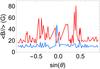 |
Fig. 1 Average unsigned magnetic flux per pixel in 20″ × 20″ regions located along the north-south polar axis as a function of the sinus of the latitude. Negative values of sinθ refer to the southern hemisphere. Red curve: 2013 data, blue curve: 2007 data. |
To select INR, we used the method described in Faurobert & Ricort (2015), which relies on line-integrated unsigned circular polarization maps of the quiet Sun measured simultaneously with the intensity maps with the SOT/SP instrument. We selected 98 INR of 10″ × 10″ located around local minima of the polarization signal.
2.1. From spectrograms to images at constant continuum optical depth
We applied the reconstruction method described in Faurobert et al. (2012) to the spectrograms to recover images of the photosphere at roughly constant continuum opacity levels above the continuum formation height. The main steps of the method are briefly recalled here.
In a spectral line the opacity, which varies steeply with the wavelength, is given by  (1)where kc is the continuum opacity, kl is the frequency-averaged line opacity, λ0 is the line center wavelength in the observer frame, and φ is the normalized absorption profile, which in the general case is given by the Voigt function, and ΔλD is the line Doppler width. In the following we use the notation δλ = (λ − λ0)/ΔλD. The Doppler broadening is due both to thermal broadening and to unresolved velocities. In the far wings, radiative and collisional damping become dominant. When the line is formed in the presence of magnetic fields, the absorption profile is also affected by the Zeeman splitting. In the quiet-Sun data we analyzed we did not observe any splitting of the line profiles, meaning that the Zeeman splitting is smaller than the Doppler broadening.
The absorption profile varies over the solar surface because of temperature, velocity, density, and magnetic inhomogeneities, and the line central wavelength varies as a results of the varying global convective motions of the matter with respect to the observer. The line central wavelength is measured from the position of the minimum of the line-intensity profile. A standard method for reconstructing images formed at various heights in the photosphere is to measure the line intensity at various values of λ − λ0. However, the corresponding line opacity varies over the solar surface because both the line absorption profile and the line strength r vary, so that such an “image” is formed at varying continuum opacity levels that span quite a broad range of depths in the atmosphere. The formation layer of the image is a very corrugated surface that is very different from a constant continuum optical depth surface. Here we wish to measure the average temperature gradient with depth in the photosphere. As explained above, we chose to measure it over layers at roughly constant continuum optical depths.
We first remark that at small line depression the shape of the intensity profile is given by I(δλ) ≃ Ic(1 − rφ(δλ)), where Ic denotes the continuum intensity. It is therefore related to the local values of r and of the line-absorption profile. When we consider for example the image obtained at 2% line-depression, it is formed at a constant continuum optical depth surface with rφ(δλ) = 0.02. The line-cord width at 2% line depression is denoted by Δλc, its value depends on r and the line absorption profile. Then considering a 1.5D-model of the solar photosphere where each pixel of the image is assumed to be formed in a 1D atmosphere with constant values of r and line-profile parameters, the ratio of line to continuum absorption coefficient at δλ = αΔλc, with α< 1, is given by rφ(αΔλc).
In the damping wings of the line the profile function decreases like 1 /δλ2, so that we have rφ(αΔλc) = (1 /α2)rφ(Δλc) = 0.02 /α2. The ratio of line to continuous absorption is thus constant over the image. In this case we can consider that the line-wing image is formed at constant continuum optical depth. This approach is valid when r and the line-absorption profile are depth-independent or do not vary significantly within the line-wing formation height. For strong lines such as the FeI 630.15 nm line, this would not apply in the line core, which is formed in the upper photosphere. In the following we shall use this image reconstruction method only in the line damping wings. To obtain a fine enough depth grid, we chose to define 25 line cords given by δλi = (i − 1)Δλc/ 24. For level indexes i larger than 15, we have rφ(δλi) ≤ 0.06. In the following we use images of the granulation obtained at line levels of between 25 and 15 to explore the depth variations of the average temperature in the low photosphere.
Figure 2 shows an example of a FeI 630.15 nm line profile with the line levels at Δλc, Δλc/ 2, Δλc/ 3, Δλc/ 4, corresponding to the line-cord indexes 25, 13, 9 and 7 respectively.
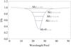 |
Fig. 2 Example of a FeI 630.15 nm line profile with the line levels corresponding to the line-cord indexes 25, 13, 9, 7 and 1. |
Faurobert et al. (2012) showed that the contrast inversion of the granulation occurs at line levels smaller than 8 for the FeI line at 630.15 nm and 7 for the 630.25 nm line.
2.2. Measurement of the image formation depth
As in Faurobert et al. (2012), we measured the perspective shift along the radial direction between images taken in a line wing and in the continuum when they are observed away from disk center (see also Grec et al. 2007, 2010).
The image obtained at a line-cord level i, denoted by Ii(x,y), is formed higher in the photosphere than the continuum image Ic(x,y). Because of the perspective effect, Ii(x,y) will appear to be shifted toward the limb in comparison with Ic(x,y) when the images are observed out of disk center. If we assume that the structures in the two images are similar, we can write 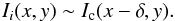 (2)By using the Fourier transform,
 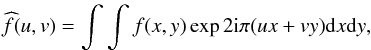 (3)relation (2) becomes in the Fourier space
  (4)The perspective displacement introduces a deterministic linear phase-term 2πδu, proportional to the spatial frequency u.
Because we use spectrograms, we have only access to the 1D brightness intensity along the slit, which is aligned with the x-axis. We therefore obtain the value of Ii(x,y) for a fixed y = y0. Two-dimensional images are not needed here because the spectrograph slit is oriented along the direction of the perspective shift. However, scanning the solar surface allows us to record many spectrograms at differenty positions to improve the statistics of the solar granulation power spectrum.
Denoting for simplicity Ii(x) the 1D cuts Ii(x,0) of the images, we can write  (5)and
  (6)Shifts can then be derived from the phase of the cross-spectrum. We used a series of spectrograms to estimate the cross-spectrum
  between Ic(x) and Ii(x):
  (7)where
  represents the conjugate Fourier transform of Ii(x), and the brackets refer to the ensemble average.
We stress here that this method allows us to measure very small displacements between images, as it is not limited by the spatial resolution of the instrument. The main limitation is the signal-to-noise ratio of the granulation spectrum and the domain of validity of Eq. (5), that is of the assumption of similarity between the line-wing and continuum images.
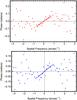 |
Fig. 3 Examples of the cross-spectrum phase for line level 15 obtained at μ = 0.80 in the southern hemisphere in a 2013 INR image (upper panel) and in a 2007 INR image (lower panel) as functions of the spatial frequency u. The lines show the linear fits of the phase in the linear domain at spatial frequencies smaller than 0.8 arcsec-1. |
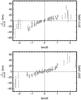 |
Fig. 4 Variation of the phase slope for line level 15 divided by cosθ as a function of the tangent of the heliocentric angle. Upper panel: 2013 data in the selected INR images, Lower panel: 2007 data in the selected INR images. The phase slope is measured in km. |
Figure 3 shows examples of the cross-spectrum phase obtained at line level 15 at μ = 0.80 in an INR in the southern hemisphere in 2013 and in 2007 (because the images are real signals the phase of the cross-spectrum is antisymmetric). We do observe a linear behavior of the phase at spatial frequencies lower than 0.8 arcsec-1 (i.e., for spatial scales larger than 1.3 arcsec). At higher frequencies the noise increases and the phase seems to oscillate around zero. There are mainly two reasons for this, the first is the limited signal-to-noise ratio of the granulation power spectrum which mainly affects high spatial frequencies, the second is that some small-scale granular features seen in the continuum image loose their coherency at higher altitudes and are not observed in the line-wing image. The phase slope is obtained from a linear fit in the interval where the linear behavior of the phase is observed. The quality of the fit, measured by the rms-dispersion of the phase points, is a source of uncertainty that is taken into account in the following.
The phase slope, that is the shift between line and continuum images, is then obtained for each line level and all the selected INR. Figure 4 shows the variations in the phase slope measured at line level 15 in the 2013 and 2007 data in all the selected INR images. For reasons that become clear in the following, we show the shift divided by the cosine of the heliocentric angle as a function of the tangent of the heliocentric angle. The positive/negative values of the heliocentric angle refer to the northern/southern hemispheres. The error bars show the one standard deviation uncertainty on the slope measurement that is due to the fluctuations of the phase within the linearity domain. We observe that the phase slope varies almost linearly with the tangent of the heliocentric angle and that it is close to zero at disk center. We also note that the slope of the linear variation is different in the northern and southern hemispheres.
We now propose an interpretation of how the measured shift behaves as a function of the heliocentric angle. A shift of the images in the plane of the sky may be due to two effects. The first is the perspective effect when the images are formed at different heights and are observed away from disk center. This effect vanishes at disk center. The second effect is a true displacement of the granular material parallel to the solar surface that is due to large scale horizontal velocities. This effect is mostly seen close to disk center. Small-scale velocity effects cancel out when we perform the ensemble averaging of the cross-spectra over surfaces of 10″ × 10″, but we may see some residual effects of supergranular velocities. According to this interpretation, the shift δ would be related to the heliocentric angle θ by  (8)where h is the formation height of the line-wing image with respect to the continuum level, and dv/// dz is the depth gradient of the horizontal velocity that induces the true displacement parallel to the surface of the granular material, and δt is the typical time for a granule to rise at height h above the base of the photosphere. Dividing Eq. (8) by cosθ, we recover the linear behavior of Fig. 4, under the condition that both h and dv/// dz do not vary with θ. Some deviations from this condition may explain the deviation from the linear curves that is observed at large heliocentric angles in Fig. 4. We measured the line formation depth h from the slope of linear fits of the (δ/ cosθ,tanθ) relation performed separately in the northern and southern hemispheres in the range − 1.2 < tanθ< 1.2 (i.e., − 50°<θ< 50°). From the δ values that we measure at the center of the solar disk, and estimating δt ≃ h/vz with vz ≃ 1 km s-1 for the vertical velocity of the granulation, we can derive the order of magnitude of hdv/// dz. We obtain values lower or on the order of 0.4 km s-1, which is consistent with the order of magnitude of supergranular velocities.
We stress that the cross-spectral method is not affected by possible image distortions, provided that the distortion is identical for the continuum and the line-wing images. When comparing measurements performed in 2007 and in 2013, we have to make sure that the pixel size in the image plane (114 km) has not changed between the two dates. Such a change would arise if the focal length of the telescope varied with time. This would also affect the apparent scale of the granulation seen in the continuum. Faurobert & Ricort (2015) showed that the power spectrum of the granulation is unchanged between the two dates except for the effect of a small defocus (0.6–0.7 mm) of the 2007 images with respect to 2013. A defocus mainly decreases the contrast of the images; this does not affect the phase of the image cross-spectrum, and the effect on the pixel size is negligible.
2.3. Continuum formation depth
The method presented above allows us to measure the formation height of line-wing images with respect to the continuum at 630 nm observed at the same heliocentric angle. We then need to evaluate the formation height of the 630 nm continuum with respect to the conventional 500 nm continuum formation height that defines the altitude z = 0 in the solar photosphere. We used the FALC standard model and the Oslo continuum opacity package to compute the formation height of the 630 nm continuum at various heliocentric angles.
The temperature gradient might be derived without referring to the standard optical depth grid, but we also intend to compare our measurements to standard quiet-Sun models. Furthermore, we also used the standard FALC model (Fontenla et al. 1999) to calibrate the brightness scale of the SOT/SP spectrograms, as we explain in the following.
2.4. Measurement of the radiation temperatures
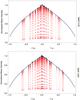 |
Fig. 5 Normalized average intensity in the images for the 25 line levels and in the continuum as functions of 1 − μ in the northern hemisphere and of − 1 + μ in the southern hemisphere. The full curve shows the fifth-order polynomial fit of the 630 nm-continuum center-to-limb variation proposed in Neckel (2005). Upper panel: 2013 data in the selected INR images; lower panel: 2007 data in the selected INR images. |
The Hinode SOT/SP instrument does not allow us to perform absolute brightness measurements, and it has also been shown that the quantum efficiency of the CCD decreases with time. Values around 0.8 were found for the loss of efficiency between 2007 and 2013 (see for example Faurobert & Ricort 2015). We therefore need to calibrate the intensity scale of the images from other data. The calibration was performed by using the average intensity in the continuum band of our spectra over seven 10″ × 10″ INR images at disk center and by computing its absolute value from the 630 nm continuum intensity at disk center with the FALC model. The same calibration procedure was applied to 2007 and 2013 data. This procedure makes use of the assumption that the continuum intensity at disk center does not vary with the solar cycle. We would have no means of detecting such variations with the Hinode SOT/SP data in any case. When the calibration was completed, we measured the average intensity in the images at the different line levels and different heliocentric angles and derived the corresponding radiation temperature. Figure 5 shows the average intensity normalized to the average continuum intensity at disk center for the different line levels and disk positions in 2013 and 2007 for the selected INR images. The full line shows the fifth-order polynomial fit of the center-to-limb variation (CLV) of the continuum mean intensity at 630 nm proposed by Neckel (2005).
Considering that the spatially averaged FeI 630.15 nm line profile is well recovered under the assumption of LTE, we identify the radiation temperature to the kinetic temperature of the medium at the image formation depth.
3. Results
Figure 6 shows the temperature measured in 2007 and 2013 in the 630 nm continuum images at varying heliocentric angles as a function of their formation depths derived from the FALC model and continuum opacity computations. The FALC model is also shown for comparison. We recall that the brightness calibration was made by adjusting the disk-center absolute intensity to the intensity and continuum optical depths obtained from the FALC model, so that it is not surprising to find a very good matching between the observed variations of the temperature and the 1D-model. However, we note that at altitudes higher than 40 km the observations show a smoother temperature gradient than the 1D quiet-Sun model. Such effects are discussed in Uitenbroek & Criscuoli (2011), where it is shown that nonlinearity in the Planck function with temperature increases the average emerging intensity of an inhomogeneous atmosphere above that of an average-property atmosphere, even if their temperature-optical depth stratification is identical.
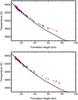 |
Fig. 6 Radiation temperature in continuum images at various positions on the solar disk as function of their formation height above the 500 nm-continuum optical depth unity. Blue dots: northern hemisphere, red stars: southern hemisphere.The full line shows the FALC quiet-Sun model. Upper panel: 2013 INR images; lower panel: 2007 INR images. |
A more model-independent determination of the temperature gradient is obtained by directly measuring the radiation temperature in a line-wing image and the image formation height above the continuum level from the perspective shift. Applying this method to the images of our INR selections in line levels 15 to 22, we obtain the results shown in Figs. 7 and 8. The results are shown separately for the northern and southern hemispheres. The measured radiation temperature is plotted as a function of the altitude z above the 500 nm-continuum formation height, so the only model-dependent quantity is the 630 nm-continuum formation height with respect to the 500 nm continuum. We cannot account for any possible cycle variations of the continuum radiation because it is calibrated by using the FALC model, as explained previously. However, the measurements performed in the line wings allow us to measure the temperature variations with z above the continuum formation height at given μ values and to investigate possible variations in the temperature gradient. We assume that the radiation temperature is well recovered from the intensity averaged over 10″ × 10″ images of the granulation, therefore we do not account for uncertainties on temperature measurements.
For completeness we present in Appendix A the measurements performed separately for the successive line levels between level 15 and 22 in the selected INR at various heliocentric angles. All these results are gathered in Figs. 7 and 8. They clearly show that below the altitude of 40 km all the measurements performed in the northern hemisphere lay below the FALC curve in 2013, whereas they are mostly above the FALC curve in 2007. It is also clear that the measurements in 2013 show an hemispheric asymmetry.
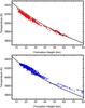 |
Fig. 7 Radiation temperature of images in the northern hemisphere, measured at line levels 15 to 22 as function of height above the 500 nm continuum optical depth unity. The full line shows the FALC quiet-Sun model. Upper panel (red symbols): 2013 INR images; lower panel (blue symbols): 2007 INR images. |
We derived average (T − z) relations from these measurements. We considered the measured (T,z) points on 5 km wide z-intervals and computed the average value of T on each interval together with the standard deviation of z and T. This is shown in Figs. 9 and 10.
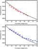 |
Fig. 9 Average value of T measured on 5 km wide z-intervals in the northern hemisphere. The bars show the standard deviation of the measurements on z and T on each interval. The full line shows the FALC quiet-Sun model. Upper panel: 2013 INR images; lower panel: 2007 INR images. |
We then computed the differences between the average value of T on each interval in the different samples and used the Student criteria to test wether the difference between two samples is statistically significant. We found statistically significant differences in 2013 between the southern and northern hemispheres, and significant differences between 2007 and 2013 in the northern hemisphere. The temperature differences between these samples are shown in Fig. 11 together with the error-bar estimates.
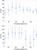 |
Fig. 11 Temperature differences derived from the average (T,z) relations. Upper panel: hemispheric difference between south and north in 2013; lower panel: difference between 2007 and 2013 in the northern hemisphere. The bars show one standard deviation on the temperature difference in each z-interval. |
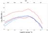 |
Fig. 12 Reduced power Fourier spectra of the unsigned magnetic flux distribution in INR at two symmetrical latitudes at ± 27°. Blue curves: in the 2007 sample; red curves: in the 2013 sample. Full lines: southern hemisphere, dashed lines: northern hemisphere. |
4. Discussion
4.1. Hemispheric asymmetry
Since the average magnetic flux shown in Fig. 1 gives no insight into the magnetic structures, we computed the power Fourier spectra of the unsigned magnetic flux in our 2007 and 2013 INR samples. This allowed us to check whether some asymmetry would be observed on the spatial distribution of the magnetic flux in INR. For these computations we divided each 10″ × 10″ INR into four 5″ × 5″ parts and performed the average of the Fourier spectra computed on these sub-regions. We furthermore averaged over seven INR located at close latitudes. In this way, we finally we obtained 2D-Fourier spectra from an average over 28 sub-regions of 5″ × 5″ located around a given latitude. Then we performed a radial averaging to obtain 1D spectra. This gives information about the spatial structuring of the magnetic flux at scales between 230 km and 3600 km. More details about Fourier power-spectra computations may be found, for example, in Faurobert & Ricort (2015). Figure 12 shows the radial average of the power spectra obtained at two symmetrical latitudes of ± 27° in the activity belt in 2007 and in 2013. As we are interested in the contrast of the magnetic flux structures we computed reduced spectra obtained by dividing the maps by their mean value before computing the power spectra. The resulting curves show how the contrast of the unsigned magnetic flux varies with the spatial scale. We note that the power spectra are roughly identical at both latitudes in 2007 and in the southern hemisphere in 2013; they show a broad maximum for scales around 700–1000 km. However, in 2013 the contrast of the magnetic flux distribution is significantly higher in the northern hemisphere. The overall shape of the spectrum does not change significantly except for a more pronounced maximum for sizes of about 730 km in 2013.
This finding may be interpreted in the following way: if we consider a given distribution of magnetic patches at different scales and if we only modify the surface density of the patches by a constant factor, then the average magnetic flux per pixel changes, but the reduced power spectrum remains unchanged. This is probably what occurs in the southern hemisphere in our 2013 INR sample.
In the northern hemisphere we observe a different phenomenon. The global increase in the contrast of the magnetic flux distribution in 2013 may be due to a change in the structure of the magnetic patches. Magnetoconvection simulations show that the typical scale of the magnetic patches increases when the ambient magnetic field increases (see, e.g., Criscuoli 2013), this could be the origin of the enhanced spectral component around 730 km observed in the northern hemisphere in 2013. A detailed study of the magnetic flux spatial distribution in the internetwork is beyond the scope of this paper, but it would certainly deserve further investigations.
Finally, we wish to point out a quite striking hemispheric asymmetry of the magnetic activity on December 7, 2013. Several large sunspots were present in the southern hemisphere, whereas the northern hemisphere appeared remarkably quiet1.
4.2. Temporal variation
Comparing the temperature gradients measured in our 2007 and 2013 datasets, we observe a steeper temperature gradient in the low photosphere in 2013 than in 2007 in the northern hemisphere and no significant change in the southern hemisphere. The values of the temperature difference shown in Fig. 11 are in qualitative agreement with the results of the MHD simulations of Criscuoli (2013) and Criscuoli & Uitenbroek (2014), when comparing snapshots embedded in regions with average magnetic fields of 100 G and 50 G. We recall that, as stated in Criscuoli 2013, MHD simulations show that around optical depth unity and below an increase of the average magnetic flux over the simulation cube causes a steepening of the temperature gradient, whereas higher up in the photosphere the effect is the opposite. The heights in the atmosphere that we observe are located in the low photosphere between z = 0 and 60 km, where the continuum optical depth is close to unity, typically between 1 and 0.8, they probably sample a region of transition between these two regimes.
4.3. Solar limb-darkening
The question now is whether the temperature-gradient variations affect the solar limb-darkening. Measurements performed at various phases of the solar cycle show that it remains remarkably constant (Elste & Gilliam 2007). We do not detect variations of the continuum intensity CLV between 2007 and 2013 either (nor hemispheric asymmetry). However, the continuum CLV reflects the variations of T with the continuum optical depth (τ). The relation between continuum optical depth and geometrical depth should vary when the temperature gradient varies because the continuum opacity, which is mainly due to H− bound-free processes, increases sharply with the temperature.
We examine a very simple analytical model where we assume that the temperature is a linear function of the geometrical depth z and the opacity varies like βT(z)α, with α ≫ 1 (high sensitivity to temperature). We consider two different atmospheres with different temperature gradients,  where T01a1 and T02a2 are the temperature depth-gradients. The optical depth is given by
 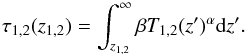 (11)At a given value of μ on the CLV curve we therefore have
 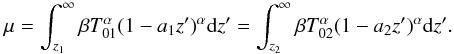 (12)This gives
 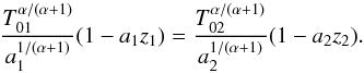 (13)When α ≫ 1 we recover T1(z1) ≃ T2(z2). In this case, the limb-darkening is identical for the two atmospheres with different temperature depth-gradients.
This example is clearly not realistic since the opacity also varies with the density and T is not a linear function of z, but it is meant to illustrate that small changes in the temperature gradients with the solar cycle may result in very small changes in the solar limb-darkening.
5. Conclusion
We used model-independent measurements of the formation-height difference between images taken in the FeI 630.15 nm line wing and in the continuum to investigate the temperature gradient in the low solar photosphere and its possible variations with the solar cycle. The height measurements performed using the cross-spectrum phase of spectrograms are not limited by the spatial resolution of the telescope, they allow precise measurements of depth differences as small as a few kilometers (corresponding to angular sizes on the order of a few hundredths of arcseconds). Furthermore, we recall that the cross-spectral method is not affected by instrumental defaults or variations of the point spread function such as image distortion or defocus.
The validity of the image reconstruction method is limited to small line depressions in the damping wings of strong absorption lines. Using the FeI line at 630.15 nm, we were able to investigate heights of 60 km at most in the low photosphere. The spatially averaged profiles of the FeI 630.15 nm line are well recovered under the assumption of LTE, therefore we may relate the radiation temperature measured in line-wing images to the kinetic temperature at their formation depth.
Our results indicate some steepening of the temperature gradient in internetwork regions of the quiet Sun at solar maximum in the northern hemisphere and no significant variation in the southern hemisphere. Comparing the spatial distribution of the INR magnetic flux in our 2007 and 2013 datasets we also found important variations of the small-scale magnetic structure in the northern hemisphere and no variation in the southern hemisphere. These findings qualitatively agree with numerical simulations of the magnetoconvection at the surface of the Sun, which also show a steepening of the temperature gradient in the low photosphere and changes in the magnetic spatial structure when the average magnetic field is increased. Variations in the magnetic pressure of the ubiquitous weak magnetic fields at very small scales in the quiet Sun might also contribute to temperature gradient variations with the solar cycle.
The measurements we carried out here need to be performed on the full irradiance data set of the Hinode satellite, which forms a complete and homogeneous set of observations starting from 2006, to confirm our results on a statistically more significant basis.
See the Hinode database at http://sdc.uio.no/search/
Acknowledgments
We thank the anonymous referee for valuable suggestions and Serena Criscuoli for useful comments on an earlier version of the manuscript and fruitful discussions. Hinode is a Japanese mission developed and launched by ISAS/JAXA, collaborating with NAOJ as a domestic partner, NASA and STFC (UK) as international partners. Scientific operation of the Hinode mission is conducted by the Hinode science team organized at ISAS/JAXA. This team mainly consists of scientists from institutes in the partner countries. Support for the post-launch operation is provided by JAXA and NAOJ (Japan), STFC (UK), NASA, ESA, and NSC (Norway). R. Balasubramanian thanks the French Ministry of Education for supporting his stay in Nice through a Charpak fellowship.
References
- Bush, R. I., Emilio, M., & Kuhn, J. R. 2010, ApJ, 716, 1381 [NASA ADS] [CrossRef] [Google Scholar]
- Criscuoli, S. 2013, ApJ, 778, 27 [NASA ADS] [CrossRef] [Google Scholar]
- Criscuoli, S., & Uitenbroek, H. 2014, ApJ, 788, 151 [NASA ADS] [CrossRef] [Google Scholar]
- Deinzer, W., Hensler, G., Schussler, M., & Weisshaar, E. 1984, A&A, 139, 435 [NASA ADS] [Google Scholar]
- Dziembowski, W. A., & Goode, P. R. 2005, ApJ, 625, 548 [NASA ADS] [CrossRef] [Google Scholar]
- Eibe, M. T., Mein, P., Roudier, T., & Faurobert, M. 2001, A&A, 371, 1128 [NASA ADS] [CrossRef] [EDP Sciences] [Google Scholar]
- Elste, G., & Gilliam, L. 2007, Sol. Phys., 240, 9 [NASA ADS] [CrossRef] [Google Scholar]
- Faurobert, M., & Ricort, G. 2015, A&A, 582, A95 [NASA ADS] [CrossRef] [EDP Sciences] [Google Scholar]
- Faurobert, M., Ricort, G., & Aime, C. 2012, A&A, 548, A80 [NASA ADS] [CrossRef] [EDP Sciences] [Google Scholar]
- Finsterle, W., Shapiro, A., Schmutz, W., & Krivova, N. 2013, in EGU General Assembly Conference Abstracts, 15, 11672 [Google Scholar]
- Fontenla, J., White, O. R., Fox, P. A., Avrett, E. H., & Kurucz, R. L. 1999, ApJ, 518, 480 [NASA ADS] [CrossRef] [Google Scholar]
- Fontenla, J. M., Harder, J., Livingston, W., Snow, M., & Woods, T. 2011, J. Geophys. Res., 116, 20108 [CrossRef] [Google Scholar]
- Fossat, E., Gelly, B., Grec, G., & Pomerantz, M. 1987, A&A, 177, L47 [NASA ADS] [Google Scholar]
- Foukal, P., & Duvall, Jr., T. 1985, ApJ, 296, 739 [NASA ADS] [CrossRef] [Google Scholar]
- Foukal, P., & Duvall, Jr., T., & Gillipsie, B. 1981, ApJ, 249, 394 [NASA ADS] [CrossRef] [Google Scholar]
- Grec, C., Aime, C., Faurobert, M., Ricort, G., & Paletou, F. 2007, A&A, 463, 1125 [NASA ADS] [CrossRef] [EDP Sciences] [Google Scholar]
- Grec, C., Uitenbroek, H., Faurobert, M., & Aime, C. 2010, A&A, 514, A91 [NASA ADS] [CrossRef] [EDP Sciences] [Google Scholar]
- Holzreuter, R., & Solanki, S. K. 2013, A&A, 558, A20 [NASA ADS] [CrossRef] [EDP Sciences] [Google Scholar]
- Kuhn, J. R., Libbrecht, K. G., & Dicke, R. H. 1988, Science, 242, 908 [NASA ADS] [CrossRef] [Google Scholar]
- Landi Degl’Innocenti, E., & Landolfi, M., ed. 2004, in Polarization in Spectral Lines, Astrophys. Space Sci. Libr., 307 [Google Scholar]
- Lefebvre, S., & Kosovichev, A. G. 2005, ApJ, 633, L149 [NASA ADS] [CrossRef] [Google Scholar]
- Lefebvre, S., Nghiem, P. A. P., & Turck-Chièze, S. 2009, ApJ, 690, 1272 [NASA ADS] [CrossRef] [Google Scholar]
- Magic, Z., Collet, R., Hayek, W., & Asplund, M. 2013, A&A, 560, A8 [NASA ADS] [CrossRef] [EDP Sciences] [Google Scholar]
- Neckel, H. 2005, Sol. Phys., 229, 13 [NASA ADS] [CrossRef] [Google Scholar]
- Riethmüller, T. L., Solanki, S. K., Berdyugina, S. V., et al. 2014, A&A, 568, A13 [NASA ADS] [CrossRef] [EDP Sciences] [Google Scholar]
- Salabert, D., García, R. A., & Turck-Chièze, S. 2015, A&A, 578, A137 [NASA ADS] [CrossRef] [EDP Sciences] [Google Scholar]
- Shchukina, N., & Trujillo Bueno, J. 2001, ApJ, 550, 970 [NASA ADS] [CrossRef] [Google Scholar]
- Solanki, S. K., Krivova, N. A., & Haigh, J. D. 2013, ARA&A, 51, 311 [NASA ADS] [CrossRef] [Google Scholar]
- Spruit, H. C. 1976, Sol. Phys., 50, 269 [NASA ADS] [CrossRef] [Google Scholar]
- Uitenbroek, H., & Criscuoli, S. 2011, ApJ, 736, 69 [NASA ADS] [CrossRef] [Google Scholar]
- Uitenbroek, H., & Criscuoli, S. 2013, Mem. Soc. Astron. It., 84, 369 [NASA ADS] [Google Scholar]
- Yeo, K. L., Krivova, N. A., & Solanki, S. K. 2014, Space Sci. Rev., 186, 137 [NASA ADS] [CrossRef] [Google Scholar]
Appendix A: Measurements at successive line levels
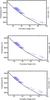 |
Fig. A.1 Measurements of the radiation temperature as a function of the line-level formation depth in the northern hemisphere in 2007 for line levels 15 to 17. The bars show the one-sigma error estimate on the measurement of the formation depth (see text). The full line shows the FALC model. |
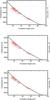 |
Fig. A.4 Measurements of the radiation temperature as a function of the line-level formation depth in the northern hemisphere in 2013 for line levels 15 to 17. The bars show the one-sigma error estimate on the measurement of the formation depth (see text). The full line shows the FALC model. |
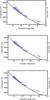 |
Fig. A.7 Measurements of the radiation temperature as a function of the line-level formation depth in the southern hemisphere in 2007 for line levels 15 to 17. The bars show the one-sigma error estimate on the measurement of the formation depth (see text). The full line shows the FALC model. |
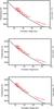 |
Fig. A.10 Measurements of the radiation temperature as a function of the line-level formation depth in the southern hemisphere in 2013 for line levels 15 to 17. The bars show the one-sigma error estimate on the measurement of the formation depth (see text). The full line shows the FALC model. |
All Figures
|
Fig. 1 Average unsigned magnetic flux per pixel in 20″ × 20″ regions located along the north-south polar axis as a function of the sinus of the latitude. Negative values of sinθ refer to the southern hemisphere. Red curve: 2013 data, blue curve: 2007 data. |
| In the text | |
|
Fig. 2 Example of a FeI 630.15 nm line profile with the line levels corresponding to the line-cord indexes 25, 13, 9, 7 and 1. |
| In the text | |
|
Fig. 3 Examples of the cross-spectrum phase for line level 15 obtained at μ = 0.80 in the southern hemisphere in a 2013 INR image (upper panel) and in a 2007 INR image (lower panel) as functions of the spatial frequency u. The lines show the linear fits of the phase in the linear domain at spatial frequencies smaller than 0.8 arcsec-1. |
| In the text | |
|
Fig. 4 Variation of the phase slope for line level 15 divided by cosθ as a function of the tangent of the heliocentric angle. Upper panel: 2013 data in the selected INR images, Lower panel: 2007 data in the selected INR images. The phase slope is measured in km. |
| In the text | |
|
Fig. 5 Normalized average intensity in the images for the 25 line levels and in the continuum as functions of 1 − μ in the northern hemisphere and of − 1 + μ in the southern hemisphere. The full curve shows the fifth-order polynomial fit of the 630 nm-continuum center-to-limb variation proposed in Neckel (2005). Upper panel: 2013 data in the selected INR images; lower panel: 2007 data in the selected INR images. |
| In the text | |
|
Fig. 6 Radiation temperature in continuum images at various positions on the solar disk as function of their formation height above the 500 nm-continuum optical depth unity. Blue dots: northern hemisphere, red stars: southern hemisphere.The full line shows the FALC quiet-Sun model. Upper panel: 2013 INR images; lower panel: 2007 INR images. |
| In the text | |
|
Fig. 7 Radiation temperature of images in the northern hemisphere, measured at line levels 15 to 22 as function of height above the 500 nm continuum optical depth unity. The full line shows the FALC quiet-Sun model. Upper panel (red symbols): 2013 INR images; lower panel (blue symbols): 2007 INR images. |
| In the text | |
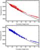 |
Fig. 8 Same as Fig. 7 for images in the southern hemisphere. |
| In the text | |
|
Fig. 9 Average value of T measured on 5 km wide z-intervals in the northern hemisphere. The bars show the standard deviation of the measurements on z and T on each interval. The full line shows the FALC quiet-Sun model. Upper panel: 2013 INR images; lower panel: 2007 INR images. |
| In the text | |
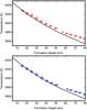 |
Fig. 10 Same as Fig. 9 for INR in the southern hemisphere. |
| In the text | |
|
Fig. 11 Temperature differences derived from the average (T,z) relations. Upper panel: hemispheric difference between south and north in 2013; lower panel: difference between 2007 and 2013 in the northern hemisphere. The bars show one standard deviation on the temperature difference in each z-interval. |
| In the text | |
|
Fig. 12 Reduced power Fourier spectra of the unsigned magnetic flux distribution in INR at two symmetrical latitudes at ± 27°. Blue curves: in the 2007 sample; red curves: in the 2013 sample. Full lines: southern hemisphere, dashed lines: northern hemisphere. |
| In the text | |
|
Fig. A.1 Measurements of the radiation temperature as a function of the line-level formation depth in the northern hemisphere in 2007 for line levels 15 to 17. The bars show the one-sigma error estimate on the measurement of the formation depth (see text). The full line shows the FALC model. |
| In the text | |
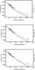 |
Fig. A.2 Same as Fig. A.1 for line levels 18 to 20. |
| In the text | |
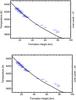 |
Fig. A.3 Same as Fig. A.1 for line levels 21 and 22. |
| In the text | |
|
Fig. A.4 Measurements of the radiation temperature as a function of the line-level formation depth in the northern hemisphere in 2013 for line levels 15 to 17. The bars show the one-sigma error estimate on the measurement of the formation depth (see text). The full line shows the FALC model. |
| In the text | |
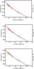 |
Fig. A.5 Same as Fig. A.4 for line levels 18 to 20. |
| In the text | |
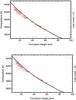 |
Fig. A.6 Same as Fig. A.4 for line levels 21 and 22. |
| In the text | |
|
Fig. A.7 Measurements of the radiation temperature as a function of the line-level formation depth in the southern hemisphere in 2007 for line levels 15 to 17. The bars show the one-sigma error estimate on the measurement of the formation depth (see text). The full line shows the FALC model. |
| In the text | |
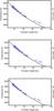 |
Fig. A.8 Same as Fig. A.7 for line levels 18 to 20. |
| In the text | |
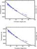 |
Fig. A.9 Same as Fig. A.7 for line levels 21 and 22. |
| In the text | |
|
Fig. A.10 Measurements of the radiation temperature as a function of the line-level formation depth in the southern hemisphere in 2013 for line levels 15 to 17. The bars show the one-sigma error estimate on the measurement of the formation depth (see text). The full line shows the FALC model. |
| In the text | |
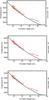 |
Fig. A.11 Same as Fig. A.10 for line levels 18 to 20. |
| In the text | |
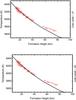 |
Fig. A.12 Same as Fig. A.10 for line levels 21 and 22. |
| In the text | |
Current usage metrics show cumulative count of Article Views (full-text article views including HTML views, PDF and ePub downloads, according to the available data) and Abstracts Views on Vision4Press platform.
Data correspond to usage on the plateform after 2015. The current usage metrics is available 48-96 hours after online publication and is updated daily on week days.
Initial download of the metrics may take a while.