| Issue |
A&A
Volume 595, November 2016
|
|
|---|---|---|
| Article Number | A124 | |
| Number of page(s) | 13 | |
| Section | Extragalactic astronomy | |
| DOI | https://doi.org/10.1051/0004-6361/201424594 | |
| Published online | 15 November 2016 | |
Constraining cloud parameters using high density gas tracers in galaxies
1 Leiden Observatory, Leiden University, PO Box 9513, 2300 RA Leiden, The Netherlands
e-mail: This email address is being protected from spambots. You need JavaScript enabled to view it.
2 Institute for Marine and Atmospheric research Utrecht, Utrecht University, Princetonplein 5, 3584 CC Utrecht, The Netherlands
3 Dipartimento di Chimica, Universitá degli Studi di Bari, via Orabona 4, 70126 Bari, Italy
4 Kapteyn Astronomical Institute, PO Box 800, 9700 AV Groningen, The Netherlands
Received: 14 July 2014
Accepted: 24 May 2016
Abstract
Far-infrared molecular emission is an important tool used to understand the excitation mechanisms of the gas in the interstellar medium (ISM) of star-forming galaxies. In the present work, we model the emission from rotational transitions with critical densities n ≳ 104 cm-3. We include 4−3 < J ≤ 15−14 transitions of CO and 13CO , in addition to J ≤ 7−6 transitions of HCN, HNC, and HCO+ on galactic scales. We do this by re-sampling high density gas in a hydrodynamic model of a gas-rich disk galaxy, assuming that the density field of the ISM of the model galaxy follows the probability density function (PDF) inferred from the resolved low density scales. We find that in a narrow gas density PDF, with a mean density of ~10 cm-3 and a dispersion σ = 2.1 in the log of the density, most of the emission of molecular lines, even of gas with critical densities >104 cm-3, emanates from the 10–1000 cm-3 part of the PDF. We construct synthetic emission maps for the central 2 kpc of the galaxy and fit the line ratios of CO and 13CO up to J = 15−14, as well as HCN, HNC, and HCO+ up to J = 7−6, using one photo-dissociation region (PDR) model. We attribute the goodness of the one component fits for our model galaxy to the fact that the distribution of the luminosity, as a function of density, is peaked at gas densities between 10 and 1000 cm-3, with negligible contribution from denser gas. Specifically, the Mach number, ℳ, of the model galaxy is ~10. We explore the impact of different log-normal density PDFs on the distribution of the line-luminosity as a function of density, and we show that it is necessary to have a broad dispersion, corresponding to Mach numbers ≳30 in order to obtain significant (>10%) emission from n> 104 cm-3 gas. Such Mach numbers are expected in star-forming galaxies, luminous infrared galaxies (LIRGS), and ultra-luminous infrared galaxies (ULIRGS). This method provides a way to constrain the global PDF of the ISM of galaxies from observations of molecular line emission. As an example, by fitting line ratios of HCN(1−0), HNC(1−0), and HCO+ (1−0) for a sample of LIRGS and ULIRGS using mechanically heated PDRs, we constrain the Mach number of these galaxies to 29 < ℳ < 77.
Key words: galaxies: ISM / photon-dominated region (PDR) / ISM: molecules / turbulence
© ESO, 2016
1. Introduction
The study of the distribution of molecular gas in star-forming galaxies provides us with an understanding of star formation processes and their relation to galactic evolution. In these studies carbon monoxide (CO) is used as a tracer of star-forming regions and dust, since in these cold regions (T< 100 K) H2 is virtually invisible. The various rotational transitions of CO emit in the far-infrared (FIR) spectrum, and are able to penetrate deep into clouds with high column densities, which are otherwise opaque to visible light. CO lines are usually optically thick and their emission emanates from the C+/C/CO transition zone (Wolfire et al. 1989), with a small contribution to the intensity from the deeper part of the cloud (Meijerink et al. 2007). On the other hand, other molecules, whose emission lines are optically thin beacuse of their lower column densities, probe greater depths of the cloud compared to CO. These less abundant molecules (e.g., 13CO) have a weaker signal than CO, and a longer integration time is required in-order to observe them. Since ALMA became available, it has become possible to obtain well-resolved molecular emission maps of star-forming galaxies in the local Universe, due to its high sensitivity, spatial and spectral resolution. In particular, many species have been observed with ALMA, including the ones we consider in this paper, namely CO, 13CO , HCN, HNC, and HCO+ (e.g., Imanishi & Nakanishi 2013; Saito et al. 2013; Combes et al. 2013, 2014; Scoville et al. 2013).
Massive stars play an important role in the dynamics of the gas around the region in which they form. Although the number of massive stars (M> 10M⊙) is about 0.1% of the total stellar population, they emit more than 99% of the total ultraviolet (FUV) radiation. This FUV radiation is one of the main heating mechanisms in the interstellar medium (ISM) of star-forming regions. Such regions are referred to as photon-dominated regions (PDRs) and they have been studied since the 1980s (Tielens & Hollenbach 1985; Hollenbach & Tielens 1999). Since then, our knowledge of the chemical and thermal properties of these regions has been improving. Since molecular clouds are almost invariably accompanied by young luminous stars, most of the molecular ISM forms in the FUV shielded region of a PDR, and thus this is the environment where the formation of CO and other molecular species can be studied. In addition, the life span of massive stars is short, on the order of 10 Myr, thus they are the only ones that detonate as supernovae, liberating a significant amount of energy into their surroundings and perturbing it. A small fraction of the energy is re-absorbed into the ISM, which heats up the gas (Usero et al. 2007; Falgarone et al. 2007; Loenen et al. 2008). In addition, starbursts (SB) occur in centers of galaxies, where the molecular ISM can be affected by X-rays of an accreting black hole (AGN) and enhanced cosmic ray rates or shocks (Maloney et al. 1996; Komossa et al. 2003; Martín et al. 2006; Oka et al. 2005; van der Tak et al. 2006; Pan & Padoan 2009; Papadopoulos 2010; Meijerink et al. 2011, 2013; Rosenberg et al. 2014a, among many others) that ionize and heat the gas.
By constructing numerical models of such regions, the various heating mechanisms can be identified. However, there is no consensus about which combination of lines define a strong diagnostic of the different heating mechanisms. This is mainly due to the lack of extensive data which would probe the various components of star-forming regions in extra-galactic sources. Direct and self-consistent modeling of the hydrodynamics, radiative transfer and chemistry at the galaxy scale is computationally challenging, thus some simplifying approximations are usually employed. In the simplest case it is commonly assumed that the gas has uniform properties, or is composed of a small number of uniform components. In reality, on the scale of a galaxy or on the kpc scale of starbursting regions, the gas density follows a continuous distribution. Although the exact functional form of this distribution is currently under debate (e.g. Nordlund & Padoan 1999), it is believed that in SB regions, where the gas is thought to be supersonically turbulent (Norman & Ferrara 1996; Goldman & Contini 2012) the density distribution of the gas is a log-normal function (Vazquez-Semadeni 1994; Nordlund & Padoan 1999; Wada & Norman 2001, 2007; Kritsuk et al. 2011; Ballesteros-Paredes et al. 2011; Burkhart et al. 2013; Hopkins 2013). This is a universal result, independent of scale and spatial location, although the mean and the dispersion can vary spatially. Self-gravitating clouds can add a power-law tail to the density PDF (Kainulainen et al. 2009; Froebrich & Rowles 2010; Russeil et al. 2013; Alves de Oliveira et al. 2014; Schneider et al. 2015). However, Kainulainen & Tan (2013) claim that such gravitational effects are negligible on the scale of giant molecular clouds, where the molecular emission we are interested in emanates.
In Kazandjian et al. (2015), we studied the effect of mechanical heating (Γmech hereafter) on molecular emission grids and identified some diagnostic line ratios to constrain cloud parameters including mechanical heating. For example, we showed that low-J to high-J intensity ratios of high density tracers will yield a good estimate of the mechanical heating rate. In Kazandjian et al. (2016), KP15b hereafter, we applied the models by Kazandjian et al. (2016) to realistic models of the ISM taken from simulations of quiescent dwarf and disk galaxies by Pelupessy & Papadopoulos (2009). We showed that it is possible to constrain mechanical heating just using J< 4−3 CO and 13CO line intensity ratio from ground based observations. This is consistent with the suggestion by Israel & Baas (2003) and Israel (2009) that shock heating is necessary to interpret the high excitation of CO and 13CO in star-forming galaxies. This was later verified by Loenen et al. (2008), where it was shown that mechanically heated PDR models are necessary to fit the line ratios of molecular emission of high density tracers in such systems.
Following up on the work done by KP15b, we include high density gas (n> 104 cm-3 ) to produce more realistic synthetic emission maps of a simulated disk-like galaxy, thus accounting for the contribution of this dense gas to the molecular line emission. This is not trivial as global, galaxy wide models of the star-forming ISM are constrained by the finite resolution of the simulations in the density they can probe. This paper is divided into two main parts. In the first part, we present a new method to incorporate high density gas to account for its contribution to the emission of the high density tracers, employing the plausible assumption, on theoretical grounds (e.g. Nordlund & Padoan 1999) that the density field follows a log-normal distribution. In the methods section, we describe the procedure with which the sampling of the high density gas is accomplished. Once we have derived a re-sampled density field we can employ the same procedure as in KP15b to model the line emission of molecular species. In Sect. 3.1, we highlight the main trends in the emission of the J = 5−4 to J = 15−14 transitions of CO and 13CO tracing the densest gas, along with the line emission of high density tracers HCN, HNC and HCO+ for transitions up to J = 7−6. In Sect. 3.2, we fit emission line ratios using a mechanically heated PDR (mPDR hereafter) and constrain the gas parameters of the model disk galaxy. In the second part of the paper, Sect. 4, we will follow the reverse path and examine what constraints can be placed on the PDF from molecular line emissions, following the same modeling approach as in the first part. We discuss the effect of the shape and width of the different density profiles on the emission of high density tracers. In particular, we discuss the possibility of constraining the dispersion and the mean of an assumed log-normal density distribution using line ratios of high density tracers. We finalize with a summary and general remarks.
2. Methods
The numerical methods we implement in this paper are similar to those in KP15b. We will focus exclusively on a single model disk galaxy, but the methods developed here could be applied to other models. We implement a recipe for the introduction of high density gas n> 104 cm-3, which is necessary to model the emission of molecular lines with critical densities1 (ncrit) in the range of 104−108 cm-3 . In the following, we summarize briefly the methods used in KP15b.
2.1. Galaxy model, radiative transfer and subgrid modelling
The model galaxy we use in this paper is the disk galaxy simulated by Pelupessy & Papadopoulos (2009), with a total mass of 1010M⊙ and a gas content representing 10% of the total mass. This represents a typical example of a quiescent star-forming galaxy. The code Fi (Pelupessy & Papadopoulos 2009) was used to evolve the galaxy to dynamical equilibrium (in total for ~1 Gyr). The simulation code implements an Oct-tree algorithm which is used to compute the self-gravity (Barnes & Hut 1986) and a TreeSPH method for evolving the hydrodynamics (Monaghan 1992; Springel & Hernquist 2002), with a recipe for star formation based on the Jeans mass criterion (Pelupessy 2005). The adopted ISM model is based on the simplified model by Wolfire et al. (2003), where the local FUV field in the neighborhood of the SPH particles is calculated using the distribution of stellar sources and population synthesis models by Bruzual & Charlot (1993, 2003) and Parravano et al. (2003). The local average mechanical heating rate due to the self-interacting SPH particles is derived from the prescription by Springel (2005): the local mechanical heating rate is estimated using the local dissipation by the artificial viscosity terms, which in this model ultimately derive mainly from the localized supernova heating. For the work presented here the most important feature of these simulations is that they provide us with the information necessary for further subgrid modeling in post-processing mode. Details about this procedure can be found in KP15b. In particular, the gas density n, the mean local mechanical heating rate Γmech, the local FUV flux G (measured in units of G0 = 1.6 × 10⁻³ erg cm-2 s-1 ) and the mean AV of the SPH particles are used. We refer to these as the main physical parameters of the gas, which are essential to parametrize the state of PDRs that are used, to obtain the emission maps. This method of computing the emission can be generally applied to other simulations, as long as they provide these physical parameters.
The PDR modeling (Meijerink & Spaans 2005) consists of a comprehensive set of chemical reactions between the species of the chemical network by Le Teuff et al. (2000). The main assumption in the extended subgrid modeling, is that these PDRs are in thermal and chemical equilibrium. We post-process an equilibrium snapshot of the SPH simulation by applying these PDR models to the local conditions sampled by each particle, and estimate the column densities of the molecules, abundances of the colliding species, and the mean gas temperature of the molecular clouds. These are the main ingredients necessary to compute the emission emanating from an SPH particle. PDR models are non-homogeneous by definition, as there are steep gradients in the kinetic temperature and the abundances of chemical species. By assuming the large velocity gradient (LVG) approximation (Sobolev 1960) using Radex (van der Tak et al. 2007), weighted quantities from the PDR models were used as input to Radex to compute the emission of the molecular species studied in this paper (Kazandjian et al. 2015). For more details on computing the emission and constructing the emission maps we refer to Sect. 2.3 of KP15b, where this method can be applied to any SPH simulation of a star-forming galaxy that provides the ingredients mentioned above. For the work in this paper, we do not include any AGN or enhanced cosmic ray physics, since these are not relevant for the simulation we have used. XDR and or enhanced cosmic ray models are necessary in modeling the ISM of ULIRGS, as was discussed by, e.g., Papadopoulos (2010) and Meijerink et al. (2011) and shown in the application of the models to Arp 299 by Rosenberg et al. (2014b).
2.2. Sampling the high-density gas
One of the main purposes of this paper is to constrain cloud parameters using the molecular transitions mentioned earlier. The typical critical densities of these transitions are between ~105 and ~108 cm-3. The highest density reached in the SPH simulation is 104 cm-3, thus the rotational levels we are interested in are subthermally populated in the non-LTE (local thermal equilibrium) regime. Therefore the intensity of the emission associated with these transitions is weak. In-order to make a more realistic representation of the molecular line emission of the ISM of the simulated galaxy, we resort to a recipe to sample particles up to 106 cm-3. In what follows, we describe the prescription we have used to sample particles to such densities.
The sampling scheme we adopt is based on the assumption that the gas density PDF of the cold neutral medium (CNM) and the molecular gas is a log-normal function, given by Eq. (1) (Press et al. 2002): ![Mathematical equation: \begin{equation} \label{eq:paper4_ln-func} \frac{{\rm d}p}{{\rm d} \ln{n}} = \frac{1}{\sqrt{2 \pi \sigma^2}} \exp{ \left( - \frac{1}{2} \left[\frac{\ln{n} - \mu }{\sigma} \right]^2 \right) } \end{equation}](/articles/aa/full_html/2016/11/aa24594-14/aa24594-14-eq45.png) (1)where μ is the natural logarithm (ln) of the median density (nmed), and σ is the width of the log-normal distribution. Such PDFs are expected in the inner (~kpc) ISM of galaxies. For example, simulations by Wada & Norman (2001) and Wada (2001) reveal that the PDF of the gas density is log-normally distributed over seven orders of magnitude for densities ranging from ~4 cm-3 to ~4 × 107 cm-3. Log-normal density distributions have been discussed by other groups as well, and we refer the reader to Sect. 1 for more references. The simulations by Wada are evolved using a grid based code with a box size ~1 kpc and include AGN feedback, whereas our simulation was evolved with an SPH code and without AGN feedback with a scale length of ~10 kpc. The major assumption in our sampling is that the gas of our model disk galaxy follows a log-normal distribution for n> 10-2 cm-3. Using this assumption we can sample and add high density gas beyond the maximum of 104 cm-3 of the simulated galaxy. Of course such re-sampling does not provide a realistic spatial distribution of high density gas, as the re-sampled particles are assumed to be placed randomly within the smoothing length of SPH particles that are dense enough to support star formation. We can use this simplification as long as we do not try to construct maps resolving scales smaller than the original spatial resolution of ~0.05 kpc.
(1)where μ is the natural logarithm (ln) of the median density (nmed), and σ is the width of the log-normal distribution. Such PDFs are expected in the inner (~kpc) ISM of galaxies. For example, simulations by Wada & Norman (2001) and Wada (2001) reveal that the PDF of the gas density is log-normally distributed over seven orders of magnitude for densities ranging from ~4 cm-3 to ~4 × 107 cm-3. Log-normal density distributions have been discussed by other groups as well, and we refer the reader to Sect. 1 for more references. The simulations by Wada are evolved using a grid based code with a box size ~1 kpc and include AGN feedback, whereas our simulation was evolved with an SPH code and without AGN feedback with a scale length of ~10 kpc. The major assumption in our sampling is that the gas of our model disk galaxy follows a log-normal distribution for n> 10-2 cm-3. Using this assumption we can sample and add high density gas beyond the maximum of 104 cm-3 of the simulated galaxy. Of course such re-sampling does not provide a realistic spatial distribution of high density gas, as the re-sampled particles are assumed to be placed randomly within the smoothing length of SPH particles that are dense enough to support star formation. We can use this simplification as long as we do not try to construct maps resolving scales smaller than the original spatial resolution of ~0.05 kpc.
In Fig. 1, we show the distributions of the gas density of our simulation along with that of the temperature. The SPH simulation consists of N = 2 × 10⁶ particles. The distribution of the temperature has a peak at low temperature and a peak at high temperature, similar to the PDF in Fig. 4 in Wada (2001). The low temperature peak around T = 300 K corresponds to gas that is thermally stable, whereas the higher temperature peak around T = 10 000 K corresponds to gas that is thermally unstable (Schwarz et al. 1972). On the other hand, the distribution of the density exhibits just one prominent peak near n ~ 1 cm-3, with a small saddle-like feature at a lower density of ~10-2 cm-3 (see the bottom panel of Fig. 1). The histogram of the density of the stable gas in the bottom panel, shows that the density of this gas ranges between 10-2<n< 104 cm-3. The lower bound of this interval is shifted towards higher densities as the gas populations are limited to lower temperatures, indicating efficient cooling of the gas for high densities. The temperature of the SPH particles represents its peripheral temperature. Thus, although the temperature might be too high for the formation of molecules at the surface, molecules could form in the PDRs present in the subgrid modeling.
The 1000 K mark seems to be a natural boundary between the thermally stable and the unstable population (see top panel of Fig. 1). Hence we use the minimum density range for this population, n ~ 10-2 cm-3, as the lower limit for the fit of the PDF that we apply. This is depicted in Fig. 2, where we fit a log-normal function to the gas density around the peak at n = 1 cm-3. The density range of the fit is nlow = 10-2<n<nhigh = 102 cm-3. To find the best fit of the actual density PDF, we examined other values for nlow and nhigh. For example, choosing nlow = 10-1 cm-3 causes the fit PDF to drop faster than the original distribution for n> 102 cm-3, which reduces the probability of sampling particles with n> 105 cm-3 to less than one particle in a sample of one billion. On the other hand, setting nhigh = 103 cm-3 does not affect the outcome of the fit. Using the best fit density PDF, we notice that only the gas within the 10-2<n< 102 cm-3 range is log-normally distributed, where the original distribution starts deviating from the log-normal fit for n> 102 cm-3 (compare blue and red curves in Fig. 2). The deviation from a log-normal distribution is likely due to the resolution limit of the SPH simulation. For example, the PDF of a simulation with 4 × 10⁵ SPH particles start to deviate from log-normality for n> 101.5 cm-3. A similar deviation in the density distribution fit by Wada (2001) is observed in the n ≳ 106 cm-3 range, most likely due to similar numerical resolution constraints. Here we will assume that the gas density will be distributed according to a log-normal function in the infinite N-limit.
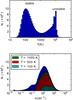 |
Fig. 1 Top: histogram of the kinetic temperature of the SPH particles. Bottom: histogram of the gas density of the SPH particles. In this same panel, the histograms for the gas densities of sub-populations of the gas are also shown. The red, green and cyan histograms correspond to gas particles with temperature below T = 1000,500,100 K respectively. These sub-populations of the gas particles are thermally stable corresponding to the peak around T = 300 K in the top panel. The vertical axis refers to the number of SPH particles within each bin. |
For each SPH particle i, parent particle hereafter, we sample from the fit PDF an ensemble { ns } of 100 sub-particles within the smoothing length of the parent, where ns and ni are the gas number densities of the sampled and parent particles respectively. The ensemble { ns } is chosen such that ns>ni, which enforces having sampled particles that are denser than the parent. The particles with n> 102 cm-3 constitute 2% of the gas mass, as their total number is ~40 000. The PDF of the sampled particles is shown in green in Fig. 2, where the sampled PDF follows the fit log-normal distribution very accurately for densities n> 103 cm-3. The bias of sampling particles with ns>ni affects the shape of the distribution between n = 102 cm-3 to 103 cm-3. This discrepancy is resolved by adjusting the weights of the sampled and parent particles along bins in density range such that the new weights match the fit PDF. These weights are used to adjust the masses of the parent and sampled particles, which ensures that the total mass of the system is conserved. The combined PDF is overlaid as black crosses in Fig. 2.
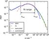 |
Fig. 2 Probability density function of the SPH particles. The blue curve corresponds to the PDF of gas density n and it is proportional to dN/ dlog (n); in other words this curve represents the probability of finding an SPH particle within a certain interval of log (n). The dashed-red curve is the log-normal fit of the PDF of the blue curve in the range 10-2 to 102. The green curve is the PDF of the sampled population from the original SPH particles while keeping the samples with n> 102 cm-3. The black crosses trace the combined PDF of the sampled and the original set of the SPH particles. The median density and the dispersion are nmed = 1.3 cm-3 and σ = 2.1 respectively. |
The re-sampling is restricted to particles with ni> 102 cm-3 to ensure that the sub-particles are sampled in regions that are likely to support star formation. Thus, most of the far-IR molecular emission results from this density range. In our sampling, we ignore any spatial dependence on the gas density distribution, where the PDFs correspond to that of all the particles in the simulation. Sampling new gas particles with n> 102 cm-3 ensures that these ensembles will lie in regions tracing CO and consequently H2. At the outskirts of the galaxy, the H2 column density is at least 100 times lower compared to the center of the galaxy. Moreover, since the density PDF is log-normal, the number of SPH particles with n> 104 cm-3 in the outskirts are so small that no emission from high density tracers is expected. Thus, we would not have enhanced molecular emission due to the sampling, e.g. for the high density tracers, at the edge of the galaxy, where it is not expected to be observed. To address this point, we examine the shape of the gas density PDF for increasing galactocentric distances. We find that the median of the log-normal distribution is shifted to lower densities, while the dispersion becomes narrower towards the edge of the galaxy. Consequently, the relative probability of finding high density gas at the outer edge of the galaxy is reduced compared to that of the central region. In fact, the PDF in the region within R< 2 kpc is closely represented by the one we have shown in Fig. 2. The dispersion of the density PDF for distances R< 2 kpc from the center is σ = 2.05 is very close to σ = 2.1 of the fit PDF in Fig. 2. On the other hand, the dispersion is σ = 1.2 for 6 <R< 8 kpc. Thus, in this paper we focus on the central region of the galaxy, where the same density PDF is used in sampling the gas particles within this region. It is worth noting that after the sampling procedure, gas with n> 104 cm-3 constitutes only 0.5% of the total gas mass. For example, this is consistent with the estimate of the filling factor of the densest PDR component derived from modeling the star-forming galaxy Arp 299 by Rosenberg et al. (2014b), even though our model galaxy is not necessarily representative of Arp 299.
The log-normality feature of the density PDF reflects non-linearity in the evolution of the gas, which we use as an argument for the cascade of turbulence into small spatial scales where high density gas forms. Here we will take the Γmech of the sampled particles to be the same as their parent SPH particle, although in (Kazandjian et al. 2015, Fig. 2) we have shown that there is some dependence of Γmech on the gas density. However, this dependence is not trivial (see Nordlund & Padoan 1999). We note that for our models Γmech would never be the dominant heating mechanism for high density gas (>104 cm-3), while this could change for modeling ULIRGs. A similar assumption was made for the AV and G of the sampled particles, where the same values as that of the parent were used. As a check we picked a typical region in the central kpc of the galaxy and quantified the mean and the standard deviation of Γmech, G and AV relative to the parent particle compared to other gas particles within its smoothing length. We found that the spread in Γmech is within a factor of two, whereas this spread decreases to within 0.1 for G and AV. Therefore, the assumption of using the same parameters as the parent for the sampled ones would have a small effect on the produced emission maps.
Various other authors have tried to overcome the resolution limit of their simulations. For example, the sampling procedure by Narayanan et al. (2008) is motivated by observations of GMCs. Their approach entails the sampling of GMCs by assuming that half of the gas mass is represented by molecules. Moreover, these GMCs are modeled as spherical and gravitationally bound with power-law density profiles provided by Rosolowsky (2005), Blitz et al. (2007) and Solomon et al. (1987). These sampling methods are similar to the work presented here, in the sense that they make a (different) set of assumptions to probe high density gas not present in the simulation. Our basic assumption is a physically motivated extension of the log-normal distribution.
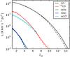 |
Fig. 3 Total luminosity of all the molecular transitions for the model galaxy over a region of 16 × 16 kpc. The dashed lines correspond to the original set of particles, whereas the solid lines represent the combined luminosity of the sampled and the original sets. |
3. Modelling dense gas in galaxy disks
3.1. Luminosity ladders and emission maps
The contribution of the high density particles to the total luminosity of each transitions is illustrated in Fig. 3. The luminosity of a SPH particle is approximated as the product of the line flux (F) with the projected area (A) of the SPH particle. The total luminosity of a certain emission line of the galaxy is computed as  , where i is the index of the SPH particles and N is the number of SPH particles. In the current implementation, the “area” of each sampled particle is assumed to be Ai/Ns, where Ns = 100 is the number of the sampled particles. This ensures that the total area of the sampled particles adds up to the area of the parent particle. Such a normalization is consistent with the SPH formalism, where all particles have the same mass. The luminosities of the lines due to the sampling are marginally affected, with a weak dependence on the transition and the species. The increase in the luminosity is due to the dependence of the flux of the emission lines on the gas density, where in general, the flux increases as a function of increasing density. The dependence of the luminosity on density and its relationship to the density PDF will be addressed in Sect. 4.
The total luminosities as a function of J, luminosity “ladders”, are computed by considering all the SPH particles within a projected box of 16 × 16 kpc. In Fig. 4 we show the flux maps of a subset of the molecular lines. These maps give insight on the regions of the galaxy where most of the emission emanates. In the next section we will use line ratios in a similar manner to KP15b in order to constrain the gas parameters within pixels in the central region of the galaxy. The rotational emission lines we have used are listed in Table 1.
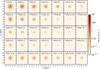 |
Fig. 4 Flux maps of the model galaxy of a selection of the CO and 13CO lines, and all of the transitions of HCN, HNC, HCO+. |
Rotational lines used in constructing the flux maps.
3.2. Constraining cloud parameters using line ratios
With the synthetic luminosity maps at our disposal, we construct various line ratios and use them to constrain the mechanical heating rate in addition to the remaining gas parameters, namely n, G and AV, throughout the central <2 kpc region of the galaxy. We follow the same approach by KP15b, where we minimize the χ2 statistic of the line ratios of the synthetic maps against these of a mechanically heated PDR model.
We fit the cloud parameters one pixel at a time and compare them to the mean physical parameters of the gas in that pixel. In Fig. 5, we show a sample fit for the central pixel of the model galaxy that has a pixel size of 0.4 × 0.4 kpc, which is the same pixel size that has been assumed by KP15b. For this fit we have considered the luminosity ladders of CO, 13CO , HCN, HNC and HCO+ normalized to the CO(1−0) transition. In addition to these, we have included the ladder of 13CO normalized to 13CO (1−0) transitions.
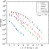 |
Fig. 5 Sample fit of the line ratios of the central pixel (0.4 × 0.4 kpc2) with a single PDR model. The points with error bars represent the line ratios of the specified species from the synthetic maps. The dashed curves correspond to the line ratios of the best fit PDR model. All the ratios are normalized to CO(1−0) except for the red ratios which are normalized to 13CO (1−0). |
The gas parameters derived from the fits for pixels of increasing distance from the center are shown in Table 2. In addition to the fit parameters, we show the mean values of these parameters in each pixel. This allows us to compare the fit values to the average physical conditions, which is not possible when such fits are applied to actual observations. We find that a mPDR constrains the density and the mechanical heating rate to less than a half-dex and the visual extinction to less than a factor of two. On the other hand, the FUV flux (G) is largely unconstrained. We note that a pure PDR that is not mechanically heated (not shown here), fails to fit most of the ratios involving J> 4−3 transitions, and leads to incorrect estimates of the gas parameters.
Model cloud parameters fits for pixels of increasing distance R (in kpc) from the center of the galaxy.
The molecular gas is indirectly affected by the FUV flux via the dust. The dust is heated by the FUV radiation, which in turn couples to the gas and heats it up. In addition to the FUV flux, this process depends also on the gas density, where it becomes very efficient for n > 104 cm-3 and G ≳ 103. In our case, the FUV flux is unconstrained mainly because the density of the gas is significantly lower than the critical densities of the J > 4−3 transitions of CO and 13CO and the transitions of the high density tracers, where 99% of the gas has a density less than 103 cm-3. These transitions are subthermally excited and their fluxes depend strongly on density. On the other hand, the emission grids of these transitions as a function of n and G show a weak dependence on the FUV flux. For example in (Kazandjian et al. 2015, Fig. 7) we show that Γmech plays a more important role in heating the gas in the molecular zone compared to the heating due to the coupling of the dust to the gas.
Despite the fact that G is not well constrained using the molecular lines we have considered, which was also the case in KP15b, we did succeed to fit the line ratios from the synthetic maps using a mechanically heated PDR. We also learn from this exercise that it is possible to constrain n, Γmech and AV with high confidence within an order of magnitude using line ratios of high density tracers as well as CO and 13CO .
It is common to have large degeneracies when using line ratios to constrain cloud parameters. Such degeneracies arise mainly due to the small number of line ratios used in the fits, while including additional line ratios reduces the degeneracy in the parameter space. Another reason to having degeneracies in the interpretation of line ratios is the assumption that the molecular lines used in these ratios emanate on average from the same spatial region of the gas. This is of-course not always true as it is evident in high resolution galactic studies (e.g., Meier & Turner 2012; Meier et al. 2014). The reduction in the degeneracies in the parameter space is illustrated in (Kazandjian et al. 2015, Fig. 16), where using four independent line ratios of a sample of LIRGS shrinks the degeneracy to less than half a dex in the n−G parameter. Possible ways of constraining G will be discussed in Sect. 5. The main reason why we manage to fit the synthetic line ratios well is because the range in the densities where most of the emission emanates is between 10 and 1000 cm-3 (see Fig. 6). This narrow range in the density is due to the narrow density PDF of our galaxy model. In the next section, we explore the effect of increasing the median and the width of the density PDF on the relative contribution of the whole span of densities to the flux of molecular line emission of mechanically heated PDRs.
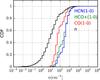 |
Fig. 6 Cumulative distribution of the densities and the luminosities of CO(1−0), HCO+ (1−0) and HCN(1−0) for the whole galaxy. For example, ~90% of the gas particles have a density n < 102 cm-3, whereas 75%, 40%, 20% of the emission of CO(1−0), HCO+ (1−0) and HCN(1−0) emanate from gas whose density is lower than 102 cm-3. |
4. Constraining the gas density PDF
The gas density PDF is a physical property of the ISM that is of fundamental interest because it gives information about the underlying physical processes, such as the dynamics of the clouds and the cooling and heating mechanisms. A log-normal distribution of the density is expected if the ISM is supersonically turbulent (Vazquez-Semadeni 1994; Nordlund & Padoan 1999; Wada & Norman 2001, 2007; Burkhart et al. 2013; Hopkins 2013), and this simple picture can explain, amongst others, the stellar IMF, cloud mass functions, and correlation patterns in the star formation (Hopkins 2012b,a, 2013). A log-normal distribution was assumed in Sect. 2 which allows us to extrapolate the density structure in the simulation beyond the resolution limit, in a statistical sense.
The question remains whether it is possible to derive the properties of the density PDF from observations. This is probably only doable for the molecular ISM. There is limited scope for deriving the density PDF of the warm and cold neutral phase of the ISM, as the HI 21 cm line is not sensitive to variations in density. For the ionized phases, we do not expect a simple log-normal density PDF, as the turbulence may not be supersonic and or the length scales exceed the scale lengths in the galaxy disk. For the colder gas, where we expect a simple functional and relatively universal form, there is at least the prospect of probing the density structure using the molecular line species, which come into play at higher densities. Indeed, we may well reverse our approach taken in Sect. 3.2, and try to constrain the density PDF (and the conditions in molecular clouds) using the emission of molecular species. Such an approach is possible because we have assembled a large database of PDR models and resulting line emission, covering a wide range of parameter space.
In the remainder of this section, we will explore a limited part of the parameter space to examine the contribution from different line species for different density PDFs under some limiting assumptions. For completeness, we recapitulate the assumptions (some of which are implicit): (1) simple functional forms of the density PDF, where G, AV and Γmech are taken constant (Nordlund & Padoan 1999); (2) emission from each density bin in the PDF is assumed to come from a PDR region at that density with a fixed AV, with the density dependence coming from emission line-width and cloud size relation (e.g, Larson 1981); (3) chemical and thermal equilibrium is assumed for the PDR models.
We have seen in Sect. 3.1 that the high density tracers, in the simulation of the quiescent disk galaxy, have a limited effect on the emission ladders. That is because the density PDF drops off very fast in the simulation. This ultimately derives from the exponential decay in the assumed log-normal distribution. For this reason, we will consider broader dispersions in the PDF. In this paper, we adopt log-normal PDFs for the density, although a more relaxed power law distribution could also be considered. Such a power law decay of the density PDF is found in some models of supersonic turbulence when the effective equation of state has a polytropic index, γ, smaller than one, and temperatures strongly decrease with increasing density (Nordlund & Padoan 1999).
4.1. Parameter study
In this section, we compute the mean flux of molecular line emission emanating from a volume of gas whose density is log-normally distributed. In the first part, we explore the contribution of gas, of increasing density, to the mean flux. Particularly, we look for the necessary parameters of the PDF to obtain a significant (>10%) contribution of the high density gas to the mean flux. In the second part, we use line ratios of HCN(1−0), HNC(1−0) and HCO+ (1−0) for star-forming galaxies to constrain the parameters of the density PDF of such systems.
In computing the mean flux for the gas in the log-normal regime, the flux emanating from gas within a certain density range, should be weighted by the probability of finding it within that range. The mean flux is computed by summing all these fluxes for all the density intervals in the log-normal regime. In other words, the mean flux for a volume of gas is given by:  where N is a normalization factor which scales the flux (
 ) depending on the molecular gas mass (M) of the region, PDF(n) is the gas density PDF we assume for the region considered, and F(n) is the emission flux of a given line as a function of gas density (for a fixed G, Γmech and AV). Typically the bounds of the integrals are dictated by the density of the molecular clouds, where the gas density is in the log-normal regime. A density of 1 cm-3 is a good estimate for the lower bound since no molecular emission is expected for gas with n less than that. The upper bound of the integral in Eq. (2) can be as high as 106–108 cm-3. PDF(n) is a Gaussian in log scale, which decays rapidly whenever the gas density is 1σ larger than the mean. While PDF(n) is a decreasing function of increasing density, F(n) is an increasing function of increasing n. Generally, the molecular gas mass in the central few kpc of star-forming galaxies is on the order of 109−1010M⊙ (Scoville et al. 1991; Bryant & Scoville 1999). This estimate, or a better one if available, can be used to compute N in Eq. (2). We refer to the quantity F(n) × PDF(n) dlnn as the weighted flux.
4.2. Weighted fluxes
The median density and the dispersion of the log-normal fit in Sect. 2 are nmed = 1.3 cm-3 and σ = 2.1 respectively, corresponding to a mean density of ~10 cm-3. The mean density is much smaller than the critical densities of most of the transitions of HCN, HNC and HCO+. For this reason all of the emission of HCN(1-0) and HCO+ (1−0) originates from gas with n< 104 cm-3 in Fig. 6. In Fig. 8, we show the weighted fluxes of gas of increasing density for HCN(1−0). The fluxes are determined by computing F in Eq. (2) for intervals in log n. Similar distributions can be computed for other emission lines of high density tracers, which are expected to be qualitatively similar. The rows in Fig. 8 correspond to the PDFs in Fig. 7. Along the columns we vary the physical cloud parameters over most of the expected physical conditions. G, Γmech and AV are varied in the first, second and last column, respectively. In exploring the possible ranges in G and Γmech for the PDF of the SPH simulation, we see that the peak of the emission is restricted to n< 103 cm-3. The only situation where the peak is shifted towards densities higher than 103 cm-3 occurs when the mean AV of the clouds in the galaxy is ~1 mag. However, in this case, the flux would be too weak to be observed. Hence with the combinations of these parameters, and with such a log-normal density PDF, it is not possible to obtain a double peaked PDF, or a gas density distribution with significant contribution from n> 104 cm-3 gas. Thus, most of the emission of the high density tracers is from gas with n< 104 cm-3. The analogous plots of Figs. 7 and 8 where the dispersion is varied for median densities of 12.5 cm-3 and 100 cm-3 are shown in Appendix A.
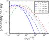 |
Fig. 7 Effect of varying the median and the dispersion of a density PDFs. The blue curves represent PDFs that have the same median density as the one used in SPH simulation, but with increasing dispersions. The green curve has the same dispersion as that of the SPH simulation but with a higher median density. Finally, the red curve corresponds to the density PDF by Wada (2001). The mean densities corresponding to these PDFs are also listed in the legend. |
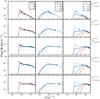 |
Fig. 8 Weighted fluxes for HCN(1−0) for different density PDFs. In the first three rows the median density of the PDFs corresponds to that of the SPH simulation, whereas the dispersion is increased from 2.1 to 2.7 to 3.5. In the fourth row, the median density is increased by a factor of 100 compared to that of the SPH simulation, but the dispersion is kept fixed at 2.1. In the last row we show the weighted fluxes for the PDF obtained by the Wada Wada (2001) simulation. In the first column the FUV flux is varied, from 100 times the flux at the solar neighborhood to 106G0 corresponding to the FUV flux in extreme starbursts (AV = 10 mag, log 10Γmech = −22). In the middle column we vary Γmech from the heating rate corresponding to quiescent disks to rates typical to violent starbursts with a SFR of 1000 M⊙ per year (AV = 10 mag, log 10G = 2). In the last column the AV is varied from 0.1 to 10 mag, corresponding respectively to the typical values for a transition zone from H+ to H and for dark molecular clouds (log 10G = 2, log 10Γmech = −22). The onset of emission is determined mainly by Γmech; for instance in looking at the middle column, we see that this onset of emission corresponds to n ~ 102 cm-3, where for lower densities H2 does not form, which is essential for other molecules such as HCN to form. For each curve in every panel we also plot (with filled circles) the density, n90, where 90% of the emission emanates from n <n90. For example, in the top row, even for the most intense FUV flux n90 ~ 103.5 cm-3. On the other hand, in bottom row, n90 > 105 cm-3. We note that the curves corresponding to Γmech 10-50 (a pure PDR) and 10-30 erg cm-3 s-1 in the second column overlap. |
For density PDFs with broader dispersions, σ = 2.7 and 3.5, respectively, it is possible to obtain luminosity distributions where at least 10% of the emission is from gas with densities >105 cm-3 (see second, third and last rows in Fig. 8). In multi-component PDF fits, the filling factor of the “denser” component is on the order of a few percent (by mass or by area). In the Fig. 8, we see that it is necessary to have a broad dispersion in the PDF in order to have a distribution of the luminosity where at least 10% of it emanates from gas with n > 105 cm-3.
When comparing the second and fourth2 rows of the weighted fluxes in Fig. 8, we see that they are quite similar. Thus, it seems that a low median density and a broad dispersion (second row) results in the same weighted fluxes as a PDF with a 100 times higher median density and a narrower dispersion (fourth row). To check for such degeneracies and constrain the PDF parameters using molecular emission of high density tracers, we construct line ratio grids as a function of nmed and σ.
It has been suggested that HCN(1−0) is a better tracer of star formation than CO(1−0) because of its excitation properties (Gao & Solomon 2004). As a proof of concept, in Fig. 9, we show a grid of line ratios of HCN(1−0)/HNC(1−0) and HCN(1−0)/HCO+ (1−0) as a function of the mean and the dispersion of the density PDF. The line ratios of a sample of 117 LIRGS (Loenen et al. 2008, Figs. 1 and 2) show that in most of these galaxies 1 ≲ HCN(1−0)/HNC(1−0) ≲ 4 and 0.5 ≲ HCN(1−0)/HCO+ (1-0) ≲ 3. The overlapping regions in the line ratio grids in Fig. 9 correspond to 2.54 < σ < 2.9. The width of a log-normal density PDF is related to the Mach number, ℳ, in that medium via σ2 ≈ ln(1 + 4ℳ2/ 3) (Krumholz & Thompson 2007; Hopkins 2012a). By applying this relationship to the range in σ constrained by the observations we find that 29 < ℳ < 77. This range in ℳ is consistent with that of violent starbursts that take place in extreme star-forming regions and galaxy centers (Downes & Solomon 1998).
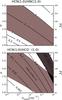 |
Fig. 9 Top: line ratios of HNC(1−0)/HCN(1−0) as a function of the mean and the dispersion of the PDF. Bottom: line ratios of HCO+ (1−0)/HCN(1−0) as a function of the mean and the dispersion of the PDF. The dark brown stripe represents observational data. The overlapping region of these two line ratios is colored in black in the bottom panel. For all the grid points a typical AV = 10 mag and Γmech = 10-22 cm-3 is used. In both panels, Mach numbers are reported on the right axes and G is 100. |
5. Discussion
The molecular emission of star-forming galaxies usually require more than one PDR component to fit all the transitions. Typically, a low density PDR components is needed to fit low-J transitions, e.g., for CO and 13CO , whereas a high density n > 104 cm-3 component is needed to fit the J> 6−5 transitions of these two species and the high density tracers. In the inner <0.1−1 kpc a mechanically heated PDR and/or an XDR might be necessary in the presence of an AGN or extreme starbursts. In the first part of the paper, we sampled high density gas in our model star-forming galaxy simulation by assuming the gas density is a log-normal function, in order to account for the emission of the high density gas that was missing in the model galaxy due to resolution constraints. Since the dispersion of the density PDF of the model galaxy is narrow with σ = 2.1, corresponding to a Mach number ℳ ~ 10, the gas with density n> 104 cm-3 contributes <1% of the total luminosity of each line. Consequently we were able to recover n, Γmech and AV of the gas parameters within 2 kpc from line ratios of CO, 13CO , HCN, HNC and HCO+, reasonably well using a one component mechanically heated PDR model. The FUV flux was constrained less accurately, since Γmech is a dominant heating term at AV ≳ 1 mag, where most of the molecular emission emanates. We have seen in Kazandjian et al. (2015) that in the non-LTE regime, the molecular emission is almost independent of the FUV flux. This is not the case for n ≳ 104 cm-3, however for such high densities the line ratio grids depend strongly on G, thus whenever the mean gas density is >104 cm-3 and G> 104, e.g. in ULIRGS, we expect to constrain the FUV flux with high certainty. In this case it might be necessary to model the emission with more than one PDR component as was done by Rosenberg et al. (2014b). In this paper, the CO ladder of the ULIRG Arp 299 was fit using three PDR models and the FUV flux was well constrained only for the densest component with n = 105.5 cm-3 (See Rosenberg et al. 2014b, Fig. 5). Another possible way of constraining G is using diagnostic line ratios of atomic fine-structure lines. Since atomic fine-structure emission originates from AV< 1 mag, it depends strongly on G. Consequently, these line ratios show a strong dependence on G as well (see review by Tielens 2013, and references therein). This is valid even for the most extreme Γmech rates (see Fig. A3 by Kazandjian et al. 2015).
Modeling the ISM as discrete components is not a realistic representation, especially in ULIRGS, since the gas in such environments is expected to be distributed log-normally and in some cases the distribution could be a power-law (depending on the adiabatic index of the equation of state).
We have studied the contribution of the density function to the mean flux for different parameters defining a log-normal probability functions and showed that a broad dispersion is required to obtain significant emission for the n> 104 cm-3 clouds. The main advantage of such modeling is in interpreting un-resolved observations of star-forming galaxies where FUV heating and mechanical heating may play an important role. This approach is more appropriate than fitting the observations with one or more PDR components, since in such modeling the gas is assumed to be uniformly distributed with discrete densities. The number of free parameters arising from multi-component fits would be much higher than fitting the parameters of the gas density PDF, which has just two. This reduces the degeneracies and gives us information on the gas density PDF and about the turbulent structure and the Mach number, which is directly related to the density PDF and the mechanical heating rate. The main caveat in our approach is the assumption that the density PDF for n> 10-2 cm-3 is a log-normal function and that the mechanical heating rate used in the PDR models is independent of the width of density PDF, AV, G and the line-width. The reason for adopting this assumption is based on the fact that a relationship between gas density, and consequently the PDF, and the mechanical heating rate is lacking (Wheeler et al. 1980; Silich et al. 1996; Freyer et al. 2003, 2006). Ultimately the mechanical heating rate derives from the cascade of turbulence to the smallest scales due to a supernova event, where typically an energy transfer efficiency of 10% is assumed (Loenen et al. 2008). The outcome of recovering cloud parameters by independently varying them in the fitting exercise is a good step towards probing possible relationships between these parameters and mechanical heating. We have demonstrated the possibility of constraining the density PDF using line ratios of HCN(1−0), HNC(1−0) and HCO+ (1−0), where the derived Mach number is consistent with previous predictions. Grids of diagnostics involving other molecular species can also be computed (see reviews by Wolfire 2011; Bergin 2011; Aalto 2014, and references therein) in order to constrain the properties of the PDF, but that is beyond the scope of this paper. Moreover, we have used the flux ratios of molecular lines as diagnostics, but it is also possible to use the ratio of the star formation rate (SFR) to the line luminosity to constrain the PDF as is done by Krumholz & Thompson (2007). This is in fact quite interesting, since the SFR can be related to the mechanical heating rate as was done by Loenen et al. (2008). By doing so, a tighter constraint on the mechanical heating rate can be imposed, instead of considering it as a free parameter as we have done in our fitting procedure.
6. Summary and conclusion
We have constructed luminosity maps of some molecular emission lines of a disk-like galaxy model. These emission maps of CO, 13CO , HCN, HNC, and HCO+ have been computed using subgrid PDR modeling in post-processing mode. Because of resolution limitations, the density of the simulation was restricted to n< 104 cm-3. We demonstrated that the density PDF is log-normal for n> 10-2 cm-3. Most of the emission of the high density tracers emanates from the gas with densities ~102 cm-3 for quiescent galaxies, which is at least 1000 times lower than the critical density of a typical high density tracer. We attribute this to the fact that the dispersion of the PDF is narrow, and thus the probability of finding dense gas is low.
The main findings of this paper are:
-
It is necessary to have a large dispersion in the density PDF(σ> 2.7) in order to have significant emission of high density tracers from n> 104 cm-3 gas.
-
It is possible to constrain the shape of the PDF using line ratios of high density tracers.
-
Line ratios of HCN(1−0), HNC(1−0), and HCO+ (1−0) for star-forming galaxies and starbursts support the theory of supersonic turbulence.
A major caveat for this approach is the assumption concerning the thermal and the chemical equilibrium. Care must be taken in interpreting and applying such equilibrium models to violently turbulent environments such as starbursting galaxies and galaxy nuclei. Despite the appealing fact that the line ratios obtained from the example we have shown in Fig. 9 favor high Mach numbers (29 < ℳ < 77) consistent with previous prediction of supersonic turbulence in starbursts, a time-dependent treatment might be essential.
We use the following definition of the critical density, ncrit ≡ kij/Aji, where kij is the collision coefficient from the level i to the level j and Aji is the Einstein coefficient (of spontaneous decay from level j to level i.
The PDF of the fourth row corresponds to that of the simulation by Wada (2001).
Acknowledgments
M.V.K is grateful to Alexander Tielens for useful comments and suggestions. M.V.K also thanks the anonymous referee and Volker Ossenkopf for their critical reviews on the manuscript that helped improve it significantly.
References
- Aalto, S. 2014, in IAU Symp. 303, eds. L. O. Sjouwerman, C. C. Lang, & J. Ott, 15 [Google Scholar]
- Alves de Oliveira, C., Schneider, N., Merín, B., et al. 2014, A&A, 568, A98 [NASA ADS] [CrossRef] [EDP Sciences] [Google Scholar]
- Ballesteros-Paredes, J., Vázquez-Semadeni, E., Gazol, A., et al. 2011, MNRAS, 416, 1436 [NASA ADS] [CrossRef] [Google Scholar]
- Barnes, J., & Hut, P. 1986, Nature, 324, 446 [NASA ADS] [CrossRef] [Google Scholar]
- Bergin, E. A. 2011, in EAS PS 52, eds. M. Röllig, R. Simon, V. Ossenkopf, & J. Stutzki, 207 [Google Scholar]
- Blitz, L., Fukui, Y., Kawamura, A., et al. 2007, Protostars and Planets V, 81 [Google Scholar]
- Bruzual, G., & Charlot, S. 1993, ApJ, 405, 538 [NASA ADS] [CrossRef] [Google Scholar]
- Bruzual, G., & Charlot, S. 2003, MNRAS, 344, 1000 [NASA ADS] [CrossRef] [Google Scholar]
- Bryant, P. M., & Scoville, N. Z. 1999, AJ, 117, 2632 [NASA ADS] [CrossRef] [Google Scholar]
- Burkhart, B., Ossenkopf, V., Lazarian, A., & Stutzki, J. 2013, ApJ, 771, 122 [NASA ADS] [CrossRef] [Google Scholar]
- Combes, F., García-Burillo, S., Casasola, V., et al. 2013, A&A, 558, A124 [NASA ADS] [CrossRef] [EDP Sciences] [Google Scholar]
- Combes, F., Garcia-Burillo, S., Casasola, V., et al. 2014, A&A, 565, A97 [NASA ADS] [CrossRef] [EDP Sciences] [Google Scholar]
- Downes, D., & Solomon, P. M. 1998, ApJ, 507, 615 [NASA ADS] [CrossRef] [Google Scholar]
- Falgarone, E., Hily-Blant, P., Pety, J., & Pineau Des Forets, G. 2007, in Molecules in Space and Laboratory, Meeting, eds. J. L. Lemaire & F. Combes, 92 [Google Scholar]
- Freyer, T., Hensler, G., & Yorke, H. W. 2003, ApJ, 594, 888 [NASA ADS] [CrossRef] [Google Scholar]
- Freyer, T., Hensler, G., & Yorke, H. W. 2006, ApJ, 638, 262 [NASA ADS] [CrossRef] [Google Scholar]
- Froebrich, D., & Rowles, J. 2010, MNRAS, 406, 1350 [NASA ADS] [Google Scholar]
- Gao, Y., & Solomon, P. M. 2004, ApJS, 152, 63 [NASA ADS] [CrossRef] [Google Scholar]
- Goldman, I., & Contini, M. 2012, in AIP Conf. Ser. 1439, eds. P.-L. Sulem, & M. Mond, 209 [Google Scholar]
- Hollenbach, D. J., & Tielens, A. G. G. M. 1999, Rev. Mod. Phys., 71, 173 [Google Scholar]
- Hopkins, P. F. 2012a, MNRAS, 423, 2016 [NASA ADS] [CrossRef] [Google Scholar]
- Hopkins, P. F. 2012b, MNRAS, 423, 2037 [NASA ADS] [CrossRef] [Google Scholar]
- Hopkins, P. F. 2013, MNRAS, 428, 1950 [NASA ADS] [CrossRef] [Google Scholar]
- Imanishi, M., & Nakanishi, K. 2013, AJ, 146, 47 [NASA ADS] [CrossRef] [Google Scholar]
- Israel, F. P. 2009, A&A, 506, 689 [NASA ADS] [CrossRef] [EDP Sciences] [Google Scholar]
- Israel, F. P., & Baas, F. 2003, A&A, 404, 495 [NASA ADS] [CrossRef] [EDP Sciences] [Google Scholar]
- Kainulainen, J., & Tan, J. C. 2013, A&A, 549, A53 [NASA ADS] [CrossRef] [EDP Sciences] [Google Scholar]
- Kainulainen, J., Beuther, H., Henning, T., & Plume, R. 2009, A&A, 508, L35 [NASA ADS] [CrossRef] [EDP Sciences] [Google Scholar]
- Kazandjian, M. V., Meijerink, R., Pelupessy, I., Israel, F. P., & Spaans, M. 2015, A&A, 574, A127 [NASA ADS] [CrossRef] [EDP Sciences] [Google Scholar]
- Kazandjian, M. V., Pelupessy, I., Meijerink, R., Israel, F. P., & Spaans, M. 2016, A&A, 595, A125 [NASA ADS] [CrossRef] [EDP Sciences] [Google Scholar]
- Komossa, S., Burwitz, V., Hasinger, G., et al. 2003, ApJ, 582, L15 [NASA ADS] [CrossRef] [Google Scholar]
- Kritsuk, A. G., Norman, M. L., & Wagner, R. 2011, ApJ, 727, L20 [NASA ADS] [CrossRef] [Google Scholar]
- Krumholz, M. R., & Thompson, T. A. 2007, ApJ, 669, 289 [NASA ADS] [CrossRef] [Google Scholar]
- Larson, R. B. 1981, MNRAS, 194, 809 [NASA ADS] [CrossRef] [Google Scholar]
- Le Teuff, Y. H., Millar, T. J., & Markwick, A. J. 2000, A&AS, 146, 157 [NASA ADS] [CrossRef] [EDP Sciences] [MathSciNet] [PubMed] [Google Scholar]
- Loenen, A. F., Spaans, M., Baan, W. A., & Meijerink, R. 2008, A&A, 488, L5 [NASA ADS] [CrossRef] [EDP Sciences] [Google Scholar]
- Maloney, P. R., Hollenbach, D. J., & Tielens, A. G. G. M. 1996, ApJ, 466, 561 [NASA ADS] [CrossRef] [Google Scholar]
- Martín, S., Mauersberger, R., Martín-Pintado, J., Henkel, C., & García-Burillo, S. 2006, ApJS, 164, 450 [NASA ADS] [CrossRef] [Google Scholar]
- Meier, D. S., & Turner, J. L. 2012, ApJ, 755, 104 [NASA ADS] [CrossRef] [Google Scholar]
- Meier, D. S., Turner, J. L., & Beck, S. C. 2014, ApJ, 795, 107 [NASA ADS] [CrossRef] [Google Scholar]
- Meijerink, R., & Spaans, M. 2005, A&A, 436, 397 [NASA ADS] [CrossRef] [EDP Sciences] [Google Scholar]
- Meijerink, R., Spaans, M., & Israel, F. P. 2007, A&A, 461, 793 [NASA ADS] [CrossRef] [EDP Sciences] [Google Scholar]
- Meijerink, R., Spaans, M., Loenen, A. F., & van der Werf, P. P. 2011, A&A, 525, A119 [NASA ADS] [CrossRef] [EDP Sciences] [Google Scholar]
- Meijerink, R., Kristensen, L. E., Weiß, A., et al. 2013, ApJ, 762, L16 [NASA ADS] [CrossRef] [Google Scholar]
- Monaghan, J. J. 1992, ARA&A, 30, 543 [NASA ADS] [CrossRef] [Google Scholar]
- Narayanan, D., Cox, T. J., Kelly, B., et al. 2008, ApJS, 176, 331 [NASA ADS] [CrossRef] [Google Scholar]
- Nordlund, Å. K., & Padoan, P. 1999, in Interstellar Turbulence, eds. J. Franco, & A. Carraminana, (Cambridge University Press), 218 [Google Scholar]
- Norman, C. A., & Ferrara, A. 1996, ApJ, 467, 280 [NASA ADS] [CrossRef] [Google Scholar]
- Oka, T., Geballe, T. R., Goto, M., Usuda, T., & McCall, B. J. 2005, ApJ, 632, 882 [NASA ADS] [CrossRef] [Google Scholar]
- Pan, L., & Padoan, P. 2009, ApJ, 692, 594 [NASA ADS] [CrossRef] [Google Scholar]
- Papadopoulos, P. P. 2010, ApJ, 720, 226 [NASA ADS] [CrossRef] [Google Scholar]
- Parravano, A., Hollenbach, D. J., & McKee, C. F. 2003, ApJ, 584, 797 [NASA ADS] [CrossRef] [Google Scholar]
- Pelupessy, F. I. 2005, Ph.D. Thesis, Leiden University, The Netherlands [Google Scholar]
- Pelupessy, F. I., & Papadopoulos, P. P. 2009, ApJ, 707, 954 [NASA ADS] [CrossRef] [Google Scholar]
- Press, W. H., Teukolsky, S. A., Vetterling, W. T., & Flannery, B. P. 2002, Numerical Recipes in C++: The Art of Scientific Computing (Cambridge University Press) [Google Scholar]
- Rosenberg, M. J. F., Kazandjian, M. V., van der Werf, P. P., et al. 2014a, A&A, 564, A126 [NASA ADS] [CrossRef] [EDP Sciences] [Google Scholar]
- Rosenberg, M. J. F., Meijerink, R., Israel, F. P., et al. 2014b, A&A, 568, A90 [NASA ADS] [CrossRef] [EDP Sciences] [Google Scholar]
- Rosolowsky, E. 2005, PASP, 117, 1403 [NASA ADS] [CrossRef] [Google Scholar]
- Russeil, D., Schneider, N., Anderson, L. D., et al. 2013, A&A, 554, A42 [NASA ADS] [CrossRef] [EDP Sciences] [Google Scholar]
- Saito, T., Iono, D., Yun, M., et al. 2013, in ASP Conf. Ser. 476, eds. R. Kawabe, N. Kuno, & S. Yamamoto, 287 [Google Scholar]
- Schneider, N., Csengeri, T., Klessen, R. S., et al. 2015, A&A, 578, A29 [NASA ADS] [CrossRef] [EDP Sciences] [Google Scholar]
- Schwarz, J., McCray, R., & Stein, R. F. 1972, ApJ, 175, 673 [NASA ADS] [CrossRef] [Google Scholar]
- Scoville, N. Z., Sargent, A. I., Sanders, D. B., & Soifer, B. T. 1991, ApJ, 366, L5 [NASA ADS] [CrossRef] [Google Scholar]
- Scoville, N., Sheth, K., Aussel, H., Manohar, S., & ALMA Cycle 0 Teams 2013, in ASP Conf. Ser. 476, eds. R. Kawabe, N. Kuno, & S. Yamamoto, 1 [Google Scholar]
- Silich, S. A., Franco, J., Palous, J., & Tenorio-Tagle, G. 1996, ApJ, 468, 722 [NASA ADS] [CrossRef] [Google Scholar]
- Sobolev, V. V. 1960, Moving envelopes of stars, Harvard books on astronomy (Harvard University Press) [Google Scholar]
- Solomon, P. M., Rivolo, A. R., Barrett, J., & Yahil, A. 1987, ApJ, 319, 730 [NASA ADS] [CrossRef] [Google Scholar]
- Springel, V. 2005, MNRAS, 364, 1105 [NASA ADS] [CrossRef] [Google Scholar]
- Springel, V., & Hernquist, L. 2002, MNRAS, 333, 649 [NASA ADS] [CrossRef] [Google Scholar]
- Tielens, A. G. G. M. 2013, Rev. Mod. Phys., 85, 1021 [NASA ADS] [CrossRef] [Google Scholar]
- Tielens, A. G. G. M., & Hollenbach, D. 1985, ApJ, 291, 722 [NASA ADS] [CrossRef] [Google Scholar]
- Usero, A., García-Burillo, S., Martín-Pintado, J., Fuente, A., & Neri, R. 2007, New Astron. Rev., 51, 75 [NASA ADS] [CrossRef] [Google Scholar]
- van der Tak, F. F. S., Belloche, A., Schilke, P., et al. 2006, A&A, 454, L99 [NASA ADS] [CrossRef] [EDP Sciences] [Google Scholar]
- van der Tak, F. F. S., Black, J. H., Schöier, F. L., Jansen, D. J., & van Dishoeck, E. F. 2007, A&A, 468, 627 [NASA ADS] [CrossRef] [EDP Sciences] [Google Scholar]
- Vazquez-Semadeni, E. 1994, ApJ, 423, 681 [NASA ADS] [CrossRef] [Google Scholar]
- Wada, K. 2001, ApJ, 559, L41 [NASA ADS] [CrossRef] [Google Scholar]
- Wada, K., & Norman, C. A. 2001, ApJ, 547, 172 [NASA ADS] [CrossRef] [Google Scholar]
- Wada, K., & Norman, C. A. 2007, ApJ, 660, 276 [NASA ADS] [CrossRef] [Google Scholar]
- Wheeler, J. C., Mazurek, T. J., & Sivaramakrishnan, A. 1980, ApJ, 237, 781 [NASA ADS] [CrossRef] [Google Scholar]
- Wolfire, M. G. 2011, in EAS PS 52, eds. M. Röllig, R. Simon, V. Ossenkopf, & J. Stutzki, 141 [Google Scholar]
- Wolfire, M. G., Hollenbach, D., & Tielens, A. G. G. M. 1989, ApJ, 344, 770 [NASA ADS] [CrossRef] [Google Scholar]
- Wolfire, M. G., McKee, C. F., Hollenbach, D., & Tielens, A. G. G. M. 2003, ApJ, 587, 278 [NASA ADS] [CrossRef] [Google Scholar]
Appendix A
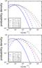 |
Fig. A.1 Analogous to Fig. 7 where the dispersion is varied for a fixed median density of 12.5 cm-3 in the top panel and 100 cm-3 in the bottom panel. In both cases the density PDF of the SPH simulation and the Wada 2001 simulation are also shown for reference and comparison. |
All Tables
Model cloud parameters fits for pixels of increasing distance R (in kpc) from the center of the galaxy.
All Figures
|
Fig. 1 Top: histogram of the kinetic temperature of the SPH particles. Bottom: histogram of the gas density of the SPH particles. In this same panel, the histograms for the gas densities of sub-populations of the gas are also shown. The red, green and cyan histograms correspond to gas particles with temperature below T = 1000,500,100 K respectively. These sub-populations of the gas particles are thermally stable corresponding to the peak around T = 300 K in the top panel. The vertical axis refers to the number of SPH particles within each bin. |
| In the text | |
|
Fig. 2 Probability density function of the SPH particles. The blue curve corresponds to the PDF of gas density n and it is proportional to dN/ dlog (n); in other words this curve represents the probability of finding an SPH particle within a certain interval of log (n). The dashed-red curve is the log-normal fit of the PDF of the blue curve in the range 10-2 to 102. The green curve is the PDF of the sampled population from the original SPH particles while keeping the samples with n> 102 cm-3. The black crosses trace the combined PDF of the sampled and the original set of the SPH particles. The median density and the dispersion are nmed = 1.3 cm-3 and σ = 2.1 respectively. |
| In the text | |
|
Fig. 3 Total luminosity of all the molecular transitions for the model galaxy over a region of 16 × 16 kpc. The dashed lines correspond to the original set of particles, whereas the solid lines represent the combined luminosity of the sampled and the original sets. |
| In the text | |
|
Fig. 4 Flux maps of the model galaxy of a selection of the CO and 13CO lines, and all of the transitions of HCN, HNC, HCO+. |
| In the text | |
|
Fig. 5 Sample fit of the line ratios of the central pixel (0.4 × 0.4 kpc2) with a single PDR model. The points with error bars represent the line ratios of the specified species from the synthetic maps. The dashed curves correspond to the line ratios of the best fit PDR model. All the ratios are normalized to CO(1−0) except for the red ratios which are normalized to 13CO (1−0). |
| In the text | |
|
Fig. 6 Cumulative distribution of the densities and the luminosities of CO(1−0), HCO+ (1−0) and HCN(1−0) for the whole galaxy. For example, ~90% of the gas particles have a density n < 102 cm-3, whereas 75%, 40%, 20% of the emission of CO(1−0), HCO+ (1−0) and HCN(1−0) emanate from gas whose density is lower than 102 cm-3. |
| In the text | |
|
Fig. 7 Effect of varying the median and the dispersion of a density PDFs. The blue curves represent PDFs that have the same median density as the one used in SPH simulation, but with increasing dispersions. The green curve has the same dispersion as that of the SPH simulation but with a higher median density. Finally, the red curve corresponds to the density PDF by Wada (2001). The mean densities corresponding to these PDFs are also listed in the legend. |
| In the text | |
|
Fig. 8 Weighted fluxes for HCN(1−0) for different density PDFs. In the first three rows the median density of the PDFs corresponds to that of the SPH simulation, whereas the dispersion is increased from 2.1 to 2.7 to 3.5. In the fourth row, the median density is increased by a factor of 100 compared to that of the SPH simulation, but the dispersion is kept fixed at 2.1. In the last row we show the weighted fluxes for the PDF obtained by the Wada Wada (2001) simulation. In the first column the FUV flux is varied, from 100 times the flux at the solar neighborhood to 106G0 corresponding to the FUV flux in extreme starbursts (AV = 10 mag, log 10Γmech = −22). In the middle column we vary Γmech from the heating rate corresponding to quiescent disks to rates typical to violent starbursts with a SFR of 1000 M⊙ per year (AV = 10 mag, log 10G = 2). In the last column the AV is varied from 0.1 to 10 mag, corresponding respectively to the typical values for a transition zone from H+ to H and for dark molecular clouds (log 10G = 2, log 10Γmech = −22). The onset of emission is determined mainly by Γmech; for instance in looking at the middle column, we see that this onset of emission corresponds to n ~ 102 cm-3, where for lower densities H2 does not form, which is essential for other molecules such as HCN to form. For each curve in every panel we also plot (with filled circles) the density, n90, where 90% of the emission emanates from n <n90. For example, in the top row, even for the most intense FUV flux n90 ~ 103.5 cm-3. On the other hand, in bottom row, n90 > 105 cm-3. We note that the curves corresponding to Γmech 10-50 (a pure PDR) and 10-30 erg cm-3 s-1 in the second column overlap. |
| In the text | |
|
Fig. 9 Top: line ratios of HNC(1−0)/HCN(1−0) as a function of the mean and the dispersion of the PDF. Bottom: line ratios of HCO+ (1−0)/HCN(1−0) as a function of the mean and the dispersion of the PDF. The dark brown stripe represents observational data. The overlapping region of these two line ratios is colored in black in the bottom panel. For all the grid points a typical AV = 10 mag and Γmech = 10-22 cm-3 is used. In both panels, Mach numbers are reported on the right axes and G is 100. |
| In the text | |
|
Fig. A.1 Analogous to Fig. 7 where the dispersion is varied for a fixed median density of 12.5 cm-3 in the top panel and 100 cm-3 in the bottom panel. In both cases the density PDF of the SPH simulation and the Wada 2001 simulation are also shown for reference and comparison. |
| In the text | |
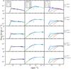 |
Fig. A.2 Weighted fluxes of the PDFs of Fig. A.1 which are not shown in Fig. 8. |
| In the text | |
Current usage metrics show cumulative count of Article Views (full-text article views including HTML views, PDF and ePub downloads, according to the available data) and Abstracts Views on Vision4Press platform.
Data correspond to usage on the plateform after 2015. The current usage metrics is available 48-96 hours after online publication and is updated daily on week days.
Initial download of the metrics may take a while.