| Issue |
A&A
Volume 594, October 2016
|
|
|---|---|---|
| Article Number | A79 | |
| Number of page(s) | 9 | |
| Section | Galactic structure, stellar clusters and populations | |
| DOI | https://doi.org/10.1051/0004-6361/201628759 | |
| Published online | 14 October 2016 | |
Abundances in a sample of turnoff and subgiant stars in NGC 6121 (M 4) ⋆,⋆⋆
1 GEPI, Observatoire de Paris, PSL Research University, CNRS, Université Paris Diderot, Sorbonne Paris Cité, Place Jules Janssen, 92195 Meudon, France
e-mail: This email address is being protected from spambots. You need JavaScript enabled to view it.
2 Departamento de Ciencias Fisicas, Universidad Andres Bello, 220 Republica, Santiago, Chile
3 Universidad de Concepción, Departamento de Astronomía, Casilla 160-C, Concepción, Chile
Received: 21 April 2016
Accepted: 28 July 2016
Abstract
Context. The stellar abundances observed in globular clusters show complex structures, currently not yet understood.
Aims. The aim of this work is to investigate the relations between the abundances of different elements in the globular cluster M 4, selected for its uniform deficiency of iron, to explore the best models explaining the pattern of these observed abundances. Moreover, in turnoff stars, the abundances of the elements are not suspected to be affected by internal mixing.
Methods. In M 4, using low and moderate resolution spectra obtained for 91 turnoff (and subgiant) stars with the ESO FLAMES-Giraffe spectrograph, we have extended previous measurements of abundances (of Li, C and Na) to other elements (C, Si, Ca, Sr and Ba), using model atmosphere analysis. We have also studied the influence of the choice of the microturbulent velocity.
Results. Firstly, the peculiar turnoff star found to be very Li-rich in a previous paper does not show any other abundance anomalies relative to the other turnoff stars in M 4. Secondly, an anti-correlation between C and Na has been detected, the slope being significative at more than 3σ. This relation between C and Na is in perfect agreement with the relation found in giant stars selected below the RGB bump. Thirdly, the strong enrichment of Si and of the neutron-capture elements Sr and Ba, already observed in the giants in M 4, is confirmed. Finally, the relations between Li, C, Na, Sr and Ba constrain the enrichment processes of the observed stars.
Conclusions. The abundances of the elements in the turnoff stars appear to be compatible with production processes by massive AGBs, but are also compatible with the production of second generation elements (like Na) and low Li produced by, for example, fast rotating massive stars.
Key words: stars: abundances / Galaxy: abundances / globular clusters: individual: M 4 / Galaxy: halo
Based on observations collected at the European Organisation for Astronomical Research in the Southern Hemisphere under ESO programme 085.D-0537(A).
Full Tables 3 and 4 are only available at the CDS via anonymous ftp to cdsarc.u-strasbg.fr (130.79.128.5) or via http://cdsarc.u-strasbg.fr/viz-bin/qcat?J/A+A/594/A79
© ESO, 2016
1. Introduction
Globular clusters provide an opportunity to improve our understanding of the problems raised by stellar nucleosynthesis. Spectroscopic and photometric observations indicate a complex structure of the stellar systems of these clusters; it is generally accepted that the observed abundances are the results of successive generations (see for example Marino et al. 2008; Villanova & Geisler 2011; Gratton et al. 2012; D’Orazi et al. 2015; Bragaglia et al. 2015), and also Bastian et al. (2015).
Measured abundances of the elements are not easy to interpret, and some further analyses of stars in globular clusters are necessary. The M 4 cluster is the nearest, enabling a detailed analysis which reveals some details in stars fainter than the stars in the giant branch.
The M 4 stars are known to have a very uniform abundance of iron (for example Carretta et al. 2009; Mucciarelli et al. 2011; Monaco et al. 2012), and a rather strong enhancement of the neutron capture elements, compared to the field stars with the same metallicity (Ivans et al. 1999; Yong et al. 2008). The red giant branch (RGB) of M 4 shows, in the U versus U−B colour diagram, two different sequences (Marino et al. 2008).
Ivans et al. (1999) and Monaco et al. (2012) have shown in giant and turnoff stars respectively, that the abundance of Na shows a large spread. Monaco et al. (2012) investigated the relation between the abundance of Na and Li. They found, for the stars hotter than 5880 K, a mean lithium abundance A(Li) = 2.13 with a very shallow slope for the Li–Na anticorrelation (we note that below 5880 K, Li is destroyed by internal stellar convection). Moreover, they detected a peculiar star with a very high Li abundance (A(Li) = 2.87 in M4-37934).
The aim of this work is to add to the work of Monaco et al. (2012) by ascertaining the abundances of some other elements, in particular the carbon abundance, in order to acquire a broader view of the abundance pattern of this cluster.
2. Observational data
Observations were conducted at the Very Large Telescope (VLT; Paranal, Chile) between April and July 2010 using the LR2 setting from 400 to 456 nm with a resolving power R = 6000, the HR12 setting from 583 to 614 nm, and the HR15N setting from 666 to 679 nm, both with a resolving power of about R = 20 000. The frames were processed using the FLAMES-GIRAFFE reduction pipeline. More information can be found in Monaco et al. (2012). The spectroscopic data are available through the Giraffe archive at Paris Observatory1.
A total of 91 stars in M 4 are discussed in the present paper. These stars span a very small interval of the HR diagram. Among them, 71 are turnoff stars with temperatures higher than 5600 K and gravities between 4.1 and 3.8. Ten other stars are subgiants and have a temperature lower than 5500 K (see the Fig. 1, in Monaco et al. 2012), and gravities (log g) between 3.5 and 3.7.
3. Spectral analysis and abundance measurements
Unlike Monaco et al. (2012) who used ATLAS models with overshooting and the MOOG code, in our analysis we used OSMARCS model atmospheres (Gustafsson et al. 2008) together with the turbospectrum synthesis code (Alvarez & Plez 1998; Plez 2012). In this code, the collisional broadening by neutral hydrogen is generally computed following the theory developed by Anstee & O’Mara (1991), Barklem et al. (2000), Barklem & O’Mara (2000).
For each star, the model parameters have been adopted from Monaco et al. (2012): the temperature is mainly based on photometry, the gravities on theoretical isochrones, and the microturbulent velocity has been chosen to obtain an abundance of Fe i independent of the equivalent width of the lines. It has been found (Monaco et al. 2012) that this microturbulence velocity decreases with the evolution of the star, from 1.7 km s-1 for the turnoff stars to 1.0 km s-1 for the subgiants.
Monaco et al. (2012) found [Fe/H] = −1.31 dex ± 0.03 for the turnoff stars and [Fe/H] = −1.17 dex ± 0.03 for the subgiants. We compared the iron abundance found with the two methods (OSMARCS models + turbospectrum and ATLAS with overshooting + MOOG) and the same model parameters in a subsample of 18 stars, and found a slight systematic difference of + 0.11 ± 0.03. Applying this correction to the Monaco et al. (2012) values, we found for the turnoff stars of the sample [Fe/H] = −1.20 dex ± 0.06 which is in good agreement with the values found by Yong et al. (2008) ([Fe/H] = −1.2), Carretta et al. (2009) ([Fe/H] = −1.2), Ivans et al. (1999) ([Fe/H] = −1.18), and Mucciarelli et al. (2011) ([Fe/H] = −1.10). However, as in Monaco et al. (2012), we found that the subgiants of the sample are systematically more metal-rich ([Fe/H] = −1.10 dex ± 0.06) than the turnoff stars.
A decrease in the microturbulence velocity between turnoff and subgiant stars is a priori, unexpected. Generally, a slight increase of the microturbulence velocity (0.2 km s-1) is observed when a star evolves from turnoff to subgiant (see e.g. Edvardsson et al. 1993). Since this decrease was based on a rather small number of iron lines we decided to investigate the consequences of a change of the microturbulence velocity adopting, as an alternative, vt = 1.3 km s-1 for all the stars (this value remains compatible with the observed spectra). In this case we found that the iron abundance in all the stars, is uniform and equal to [Fe/H] = −1.16 dex ± 0.06.
It is important to note that in Monaco et al. (2012), the lithium abundance has been directly derived from the equivalent width of the Li i resonance doublet at 670.8 nm using the Sbordone et al. (2010) formula B.1 based on 3D models and non local thermodynamical equilibrium (NLTE) computations. As a consequence, the lithium abundance is not affected by the difference of the model grids used in Monaco et al. (2012) nor by the microturbulence velocity. In the discussion we adopted the lithium abundances given by Monaco et al. (2012) in their Table A.1. For all the other elements the abundances have been computed with the microturbulence velocity given in Monaco et al. (2012; option A), and with vt = 1.3 km s-1 (option B). The impact of a change in the microturbulent velocity depends on the equivalent widths of the lines. It has practically no effect on weak or very strong lines but is maximum around 100 mÅ. The effect is often the same on the element “X” and on the iron abundance, in this case [X/Fe] does not change.
3.1. Carbon abundance
The carbon abundance has been computed by fitting the computed profile of the CH G-band (A2Δ−X2Π) to the observed spectrum between 426 and 431.6 nm. Line lists for 12CH and 13CH (Masseron et al. 2014) were included in the synthesis. The carbon abundances were computed independently adopting the microturbulence velocity given by Monaco et al. (2012), and also vt = 1.3 km s-1. The CH band is not very sensitive to a change of the microturbulence velocity and the difference in A(C) between the two options never exceeds 0.1 dex, it is about +0.02 dex for the subgiants and –0.01 dex for the turnoff stars. In Fig. 1 we present the fit of the spectra for two typical stars in M 4 computed with the microturbulence velocity given by Monaco et al. (2012).
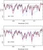 |
Fig. 1 Observed profile of the CH band in M4-1024 and M4-37934 (black line). In both cases synthetic profiles (blue thin lines) have been computed with A(C) = 6.4 6.9 7.4. The thick red line represent the best fit (1D computations) A(C) = 6.6 for M4-1024 and A(C) = 7.0 for M4-37934. |
The CH band is formed in a region of the atmosphere close to the surface where the effects of stellar convection can be important. Three dimensional (3D) dynamic model atmospheres (CIFIST models based on the CO5BOLD code: Ludwig et al. 2009; Freytag et al. 2012) were used to compute spectral synthesis and test the role of the granulation in the formation of the G-band (Gallagher et al. 2016). The models they investigated have atmospheric parameters of turnoff stars, close to the stars of M 4 analysed here. We were able to interpolate corrections from their Table 2 to derive a 3D correction to apply to the C abundance derived here. This correction A(C)3D−A(C)1D, is very small: approx. +0.03 dex for the M 4 turnoff stars and +0.05 dex for the subgiants.
3.2. Sodium abundance
Using the OSMARCS model atmospheres and turbospectrum, we computed the profiles of the sodium D lines. Applying the NLTE correction computed by S. Andrievsky and S. Korotin (as in Monaco et al. 2012), we found a very small systematic difference with the values published by Monaco et al. (2012): ΔA(Na) = −0.06 dex ± 0.06 but the scatter of [Na/Fe] remains the same.
The strong sodium D lines are not very sensitive to a change of the microturbulence velocity and as a consequence a change of the microturbulent velocity does not change the scatter of [Na/Fe].
We estimate that the error in the A(Na) measurement is about 0.1 dex.
It is interesting to note that also in metal-poor turnoff field stars, the abundance of Na at this metallicity is scattered (see e.g. Gehren et al. 2006).
3.3. Silicon abundance
The silicon abundance has been deduced from only the Si i line at 594.855 nm (Table 1). The resolving power of the spectrum in this region is close to 20 000 and the S/N per pixel, is between 55 and 85. The equivalent width (EW) of the Si i line is between 25 and 70 mÅ and thus the silicon abundance is sensitive to the microturbulence velocity. The expected uncertainty in the measured equivalent width can be estimated by the Cayrel formula (Cayrel 1988): 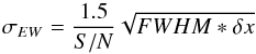 (1)where S/N is the signal-to-noise ratio per pixel, FWHM the full width of the line at half maximum, and δx the pixel size. For a typical S/N ratio of 70 per pixel the predicted accuracy σEW is about 3 mÅ. However this formula neglects the uncertainty on the continuum placement. After varying slightly the continum level within the range allowed by the S/N of the spectra, we estimated that the accuracy in the measurement of the equivalent width of the Si i line is about 6 mÅ. This uncertainty corresponds to an uncertainty of about 0.1 dex in [Si/Fe] but it relies on only one log gf value classified as quality C (σ(gf) ≤ 25%), in the NIST data base (Reader et al. 2012).
Main characteristics of the atomic lines used in the present analysis.
3.4. Calcium abundance
The calcium abundance was deduced from the fit of the profile of four Ca lines (Table1). For each star, the accuracy of the Ca abundance was estimated from the standard deviation of these four abundances around the mean value, the mean standard deviation is close to ≈0.11 dex. The equivalent widths of the four Ca i lines are close to 100 mÅ and thus are sensitive to the microturbulence velocity. The calcium lines are also sensitive to NLTE effects. The NLTE corrections have been computed by S. Andrievsky and are available in Spite et al. (2012)2. For the Ca lines used in the present paper this NLTE correction is close to –0.11 dex.
3.5. Nickel abundance
The nickel abundance was estimated from the equivalent width of only one line (Table 1) as was done for silicon. The equivalent width of this Ni line varies from star to star, between 14 and 70 mÅ, the strongest lines are thus sensitive to a change of the microturbulence velocity. We took into account only the Ni lines that had an equivalent width larger than 20 mÅ. In this region of the spectrum, the resolving power of the spectra is close to 20 000 and the S/N ratio per pixel is between 50 and 100, with a typical value of about 70. From the Cayrel formula (see Sect. 3.3) we found σEW ≈ 3 mÅ, and 6 mÅ taking into account the uncertainty on the position of the continuum. With a typical equivalent width of 30 mÅ this value corresponds to an uncertainty in [Ni/Fe] of about 0.14 dex. Moreover the Ni abundance relies on only one log gf value classified as quality D (σ(gf) ≤ 50%) in the NIST data base (Reader et al. 2012).
3.6. Strontium abundance
The strontium abundance has been estimated from the fit of the observed spectrum around the Sr line at 407.77 nm with a synthetic spectrum computed with turbospectrum. The observed spectrum in the region of the Sr line only has a resolving power R = 6000, an example of the fit is given in Fig. 2. The uncertainty of the measurement of [Sr/Fe] is estimated to be as large as 0.25 dex.
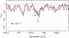 |
Fig. 2 Observed profile of the feature around the Sr ii line (black line). Three synthetic profiles (blue thin lines) have been computed with abundances A(Sr) = 1.9, 2.2, 2.5 and one with no strontium (dashed blue line). The thick red line represent the best fit (LTE computations) with A(Sr) = 2.1 for the star M4-32111. |
3.7. Barium abundance
We derived the abundance of Ba from the fitting of three Ba features taking into account the hyperfine structure of the lines (Table 1). For twelve stars the standard deviation is equal or larger than 0.30. These stars have not been taken into consideration. Moreover, for nine other stars only the “blue” low resolution spectra (setting LR2) were available and thus the Ba abundance has been estimated only from the resonance line at 455.4 nm and we estimate that for these stars the stochastic uncertainty can reach 0.25 dex. For the other 70 stars the mean standard deviation is equal to 0.15 dex.
3.8. Error budget
Uncertainties in the abundance measurements include those related to the adopted oscillator strengths, to the equivalent widths or profile measurements and to the adopted stellar parameters. The error on the oscillator strengths is difficult to assess and can be particularly important when the element is represented by a very small number of lines. However, since this error is the same for all the stars, it can produce only a general shift in the abundance of the element (the same for all the stars).
The adopted measurement errors are given for each element in Sects. 3.2 to 3.7.
The computations of the error linked to our choice of the stellar parameters (Table 2) have been done for a star with Teff = 5950 K and log g = 4.0 (model A). A change of –100 K of the temperature corresponds to model B. Since gravity has been estimated with the aid of theoretical isochrones (Monaco et al. 2012), a change of temperature of –100 K would induce an automatic change of log g of –0.1 dex (model C). A comparison of the results obtained with models A and B, and B and C, allows an estimation of the error induced by a variation of Teff and log g alone. A comparison of the results obtained with models C and A shows the global consequences of a change of –100 K in the temperature of the stars: it does not significantly affect the ratios [X/Fe] when atomic lines are used (for Na, Si, Ca, Ni, Sr, Ba). But [C/Fe], based on the study of the CH band, decreases by 0.13 dex.
For each element X, the total uncertainty on the relative abundance [X/Fe] is computed as the quadratic sum of the stochastic and systematic errors. The total uncertainty is dominated by the measurement errors, since errors in the model parameters largely cancel each other out in the measured ratios of the elements.
Abundances uncertainties linked to stellar parameters.
4. Discussion
Tables 3 and 4 tabulate the abundances of lithium, carbon, sodium, silicon, calcium, strontium and barium relative to iron in our sample of turnoff and subgiant stars, adopting respectively the microturbulence velocity given in Monaco et al. (2012; option A) and vt = 1.3 km s-1 (option B). In this last case we adopted for all the stars [Fe/H] = −1.16 dex since the measurement errors exceeded the measured scatter. For several elements the effect of a variation of the microturbulence velocity on the abundance is about the same as it is for Fe and thus [X/Fe] is little affected.
For Li and Na the abundances given in the tables take into account the NLTE effects. The sodium abundance has been determined from the resonance lines and thus the NLTE correction is large and it is different from star to star since it depends on the equivalent width of the Na lines. In order to compare with the Na abundances in the literature, generally estimated from the secondary lines, that are less affected by NLTE effects, this correction has to be carefully taken into account. Since generally in the literature the Ca and Ba abundances are not corrected for NLTE effects, we kept in the tables the LTE Ca and Ba abundances for an easier comparison. When possible, an estimation of the NLTE effects is given in the discussion.
Abundances measured in our sample of M 4 stars computed with the model parameters Tefflog g and vt given by Monaco et al. (2012).
Abundances measured in our sample of M 4 stars computed with the model parameters Tefflog g given by Monaco et al. (2012) but with vt = 1.3 km s-1.
4.1. Relation between the abundances of C and Na
In globular clusters the abundances are often measured in bright giants. But in giant stars the carbon abundance may be affected by mixing with deep layers processed by the CNO cycle. Carbon abundances in turnoff stars, however, should be an indisputable measurement of the C abundance in the gas cloud that formed the star.
In Fig. 3 we present the variation of the carbon abundance [C/Fe] in the M 4 turnoff stars and the subgiants as a function of [Na/Fe] with the two different choices of the microturbulence velocity (options A and B). This figure includes the NLTE correction for the Na abundance and the weak 3D correction for the carbon abundance (see Tables 3 and 4). Two turnoff stars appear to be very carbon-poor (and slightly Na-rich): M4-1024 and M4-39862.
If we ignore these two C-poor stars, an anti-correlation between C and Na is observed in the turnoff stars (slope − 0.32, correlation factor − 0.51 when the microturbulence velocity given in Monaco et al. 2012 is adopted, and a slope − 0.43, with a correlation factor − 0.59 when vt =1.3 km s-1 is adopted). A non parametric test (Kendall’s tau) shows that the probability of correlation is better than 99.98%.
In Fig. 3A the subgiant stars seem to have, as a mean, a carbon abundance systematically 0.1 dex lower than the turnoff stars with the same value of [Na/Fe] (if we ignore the two C-poor turnoff stars). However this effect disappears (Fig. 3B) when a microturbulent velocity vt = 1.3 km s-1 is adopted for subgiant and turnoff stars.
In these figures the subgiant stars all have a positive value of [Na/Fe], but this effect is spurious. In our sample, there is at least one subgiant (M4-33548) which has a lower value of [Na/Fe]: − 0.06 ± 0.15, unfortunately we could not measure the carbon abundance of this star and thus it does not appear in Figs. 3A and B (but it is visible on the subsequent figures).
A sample of RGB stars located below the RGB bump, has been studied in M 4 by Villanova & Geisler (2011). They found a correlation between [C/Fe] and [Na/Fe], interpreted as the result of the existence of two different populations. Their sample is divided in two subsamples: the first one with the C-rich N-poor stars and the second one with the C-poor N-rich stars. In Fig. 3A and B we plotted the mean Na abundance of these two groups of giants as a function of the mean value of [C/Fe] (the black open stars symbols). The agreement between turnoff stars and RGB stars is excellent.
The position in the diagram of the very Li-rich turnoff star M4-37934 (Monaco et al. 2012), is surrounded by a red circle in Fig. 3 to Fig. 7, this star has a normal carbon abundance compared to the other turnoff stars with the same value of [Na/Fe].
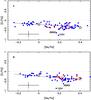 |
Fig. 3 Relation between [C/Fe] and [Na/Fe] computed, A) with the model parameters Tefflog g and vt given in Monaco et al. (2012), and B) with the same parameters but vt =1.3 km s-1. The red squares represent the subgiant stars which have a temperature below 5600 K. The blue dots are for the turnoff stars with 5600 K < Teff < 5980 K. The very Li-rich star M4-37934 is surrounded by a red circle. A typical value of the total error is represented by the cross at the lower left corner of the figure. The mean values obtained for the two groups of RGB stars in M 4 by Villanova & Geisler (2011): C-rich N-poor stars and the C-poor N-rich stars are shown by black open stars symbols. |
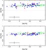 |
Fig. 4 Relations between the abundances of the α elements Si (upper panel) and Ca (lower panel) vs. [Na/Fe]. The symbols are as in Fig. 3. In these two figures we compare the abundance measured in the turnoff stars to the abundances measured by Ivans et al. (1999), Marino et al. (2008) and Villanova & Geisler (2011) in samples of bright giants (respectively green +, × and □). The α-elements Si and Ca are overabundant relative to iron. |
4.2. Abundances of α-elements: [Si/Fe], [Ca/Fe] vs. [Na/Fe]
The relations of [Si/Fe] and [Ca/Fe] versus [Na/Fe] are displayed in Fig. 4 for the microturbulence velocity of Monaco et al. (2012). Silicon and Calcium are overabundant relative to iron in M 4 turnoff and subgiant stars. The mean overabundance of silicon is [Si/Fe] = +0.51 dex if the vt of Monaco et al. (2012) is adopted, and [Si/Fe] = +0.48 if vt = 1.3 km s-1, but since this measurement is based on only one silicon line with a rather uncertain log gf value, this result could be affected by a systematic error. However, Villanova & Geisler (2011), Yong et al. (2008), Marino et al. (2008) and Ivans et al. (1999) also found a similar high abundance of silicon based on more Si lines ([Si/Fe] = +0.43, [Si/Fe] = +0.58, [Si/Fe] = +0.48 and +0.55), in the bright giants of M 4.
Contrary to this, (with the two different values of vt), we found a rather low mean overabundance of Ca: [Ca/Fe] = +0.18 close to the mean value found by Ivans et al. (1999): [Ca/Fe] = 0.26, or Marino et al. (2008): [Ca/Fe] = 0.28, while Yong et al. (2008) and Villanova & Geisler (2011) found in M 4 [Ca/Fe] = +0.41.
There is no trend of [Ca/Fe] vs. [Na/Fe]. A positive correlation between [Si/Fe] and [Na/Fe] is possible, but there is a large scatter in [Si/Fe] and the slope is not significant.
The values of [Si/Fe] and [Ca/Fe] in the Very Li-rich star M4-37934, are similar to the values found for the other M 4 turnoff stars.
4.3. Ni abundances vs. [Na/Fe]
We found a slight overabundance of nickel in the turnoff and subgiant stars in M 4: [Ni/Fe] = + 0.16 ± 0.10 if for vt the value given by Monaco et al. (2012) is adopted and [Ni/Fe] = 0.14 ± 0.10 if vt = 1.3 km s-1. There is no significant trend with [Na/Fe] (Fig. 5). Taking into account that our determination of the Ni abundance is based on only one line with a rather uncertain log gf (see Sect. 3.5), this mean value is in fair agreement with the values found in giants by Ivans et al. (1999) [Ni/Fe] = +0.05; Marino et al. (2008) [Ni/Fe] = +0.02; Villanova & Geisler (2011)[Ni/Fe] = −0.01. It is in very good agreement with the value found by Yong et al. (2008): [Ni/Fe] = +0.12 (these last data could not be plotted on the Fig. 5 because the sodium abundance has not been measured in the sample of Yong et al. 2008).
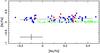 |
Fig. 5 Relation between the abundance of the iron peak element [Ni/Fe] vs. [Na/Fe]. The symbols are the same as in Fig. 3. |
4.4. Heavy elements abundances: Sr and Ba vs. [Na/Fe]
The cluster M 4 is known to be rich in neutron-capture elements like Sr and Ba. For our sample of turnoff and subgiant stars we found that, if we adopt the microturbulence velocity of Monaco et al. (2012), the mean value of [Ba/Fe] is equal to + 0.33 ± 0.13 (Fig. 6A), and + 0.45 ± 0.13 with vt =1.3 km s-1 (Fig. 6B) .
These values are in good agreement with Marino et al. (2008) who found in giants below the bump [Ba/Fe] = + 0.41. Ivans et al. (1999) found a higher value of the abundance of Ba: ([Ba/Fe] = 0.60 dex ± 0.10) but they studied a more evolved sample of giants and the NLTE correction can be higher for these stars.
We interpolated in the grid of Korotin et al. (2015) the NLTE corrections of the Ba abundance for our sample of turnoff stars and for a typical evolved giant. The mean correction is about − 0.05 dex for turnoff stars and − 0.15 dex for giants. Taking these corrections into account the main [Ba/Fe] value in our sample of turnoff stars is +0.28 dex, or +0.40 with vt = 1.3 km s-1 and it is +0.45 dex in the sample of giant stars studied by Ivans et al. (1999). These values are compatible within the errors.
In our sample of stars we measured [Sr/Fe] = + 0.37 ± 0.13 adopting the microturbulence velocity of Monaco et al. (2012), and [Sr/Fe] = + 0.41 ± 0.13 with vt =1.3 km s-1. Yong et al. (2008) found a significantly higher value of the abundance of Sr ([Sr/Fe] = 0.73 dex ± 0.10) in their sample of giants. But here again the difference can reflect the fact that the results of the LTE computations of the abundance of Ba are not affected in the same way by the NLTE effects when stars are dwarfs or giants. However our measurement of the strontium abundance is based on the profile of a complex feature (see Fig. 2) and should be affected by neighbouring lines.
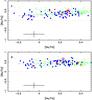 |
Fig. 6 Relation between [Ba/Fe] and [Na/Fe] computed with A) vt from Monaco et al. (2012), and B) vt = 1.3 km s-1. The symbols are the same as in Fig. 4. |
No significant trend is observed between the abundance of Na and the abundances of Sr or Ba (Figs. 6 and 7). However a difference of 0.2 dex in [Sr/Fe] between the Na-poor stars and the Na-rich stars, like the difference observed for Y in the giants by (Villanova & Geisler 2011, their Fig. 5, lower panel), cannot be excluded. One star M4-60462 seems to have a weak strontium feature but the abundance of barium is normal in this star. One more spectrum would be useful to confirm this anomaly.
4.5. Lithium abundance vs. [Na/Fe] and [C/Fe]
4.5.1. Subgiant stars
Low-mass stars leaving the main sequence develop surface convection zones, which deepen when the star continues to evolve. The surface convection mixes the surface layer with deeper material in which lithium has been depleted. Monaco et al. (2012) and Mucciarelli et al. (2011) have shown that the Li abundance decreases in M 4 subgiant stars with decreasing stellar effective temperature. This decline of A(Li) (Fig. 8) is the same in NGC 6397 (Korn et al. 2007) and in field stars with about the same metallicity as M 4 (see e.g. Pilachowski et al. 1993). The combined effects of diffusion and convection are expected to explain the decrease of A(Li) but Mucciarelli et al. (2011) were not able to reproduce the general behaviour of Li and Fe with Teff in M 4 (from turnoff stars to giants) starting with the cosmological lithium abundance predicted by WMAP+BBNS.
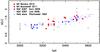 |
Fig. 8 Variation of the lithium abundance in evolved stars in M 4, NGC 6397, and field metal-poor stars as a function of the effective temperature. |
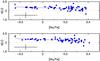 |
Fig. 9 A(Li) vs. [Na/Fe] for turnoff stars selected in our sample within a very small interval of temperature: 5880 ≤ Teff ≤ 5980 K and computed with A)vt from Monaco et al. (2012), and B) vt = 1.3 km s-1. |
4.5.2. Turnoff stars
In Figs. 9 and 10 we selected, as in Monaco et al. (2012), only stars in the temperature interval 5880 ≤ Teff ≤ 5980 K and we excluded the peculiar Li-rich star M4-37934 (70 stars are taken into account).
It has been shown (in Fig. 9 and Monaco et al. 2012) that the cluster stars in this sample display a mild but statistically significant Li–Na anticorrelation, at variance with the stars in NGC 6752 (Pasquini et al. 2005) where the anticorrelation is strong, and the turnoff stars in NGC 6397 (González Hernández et al. 2009; Lind et al. 2009) where no anticorrelation is observed.
When the lithium abundance is plotted versus [C/Fe] (Fig. 10) for the same sample of stars, a mild correlation is observed (correlation coefficient +0.30): A(Li) increases slightly with [C/Fe]. This behaviour is expected since the abundances of C and Na are anticorrelated (Fig. 3).
A change of the microturbulence velocity (panels A and B of Figs. 9 and 10) does not induce a significant change in the relations A(Li) vs. [Na/Fe] and A(Li) vs. [C/Fe].
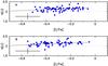 |
Fig. 10 A(Li) vs. [C/Fe] for turnoff stars selected in our sample within a very small interval of temperature: 5880 ≤ Teff ≤ 5980 K and with A) vt from Monaco et al. (2012) and B) vt = 1.3 km s-1. |
5. Conclusions
The abundances of C, Si, Ca, Ni, Sr, Ba have been measured in a sample of M 4 subgiant and turnoff stars, previously analysed for Li by Monaco et al. (2012).
-
In this paper all the abundance determinations have been donewith two options for the microturbulence velocity. In the firstoption (A) we adopted the same microturbulence velocity asin Monaco et al. (2012) and inthe second (B) we adopted vt = 1.3 km s-1 for all the turnoff and subgiant stars. With the hypothesis A,as in Monaco et al. (2012), wefound that [Fe/H] is higher (by 0.1 dex) insubgiant stars than in turnoff stars. This effect disappears if aconstant microturbulence velocity is adopted for all the starsof the sample (option B). In this case [Fe/H] is found to be close to− 1.16 ± 0.06 dex for all the stars. The relation A(Li) vs. [Na/Fe] and A(Li) vs. [C/Fe] are practically the same with the hypotheses A and B for the microturbulence velocity.
-
2.
In Fig. 3 the distribution of the dots suggest the existence of two subgroups of stars, one “Na-poor C-rich”, and one “Na-rich C-poor”, as also noted in giants by Marino et al. (2008) and Villanova & Geisler (2011) linking this difference to observed photometric differences, recently confirmed by Piotto et al. (2015).
-
3.
We confirm the enhancement of the heavy elements Sr and Ba previously found in giant stars. This enhancement has been found to be less important in turnoff or subgiant stars than in highly evolved giant stars (Ivans et al. 1999; Yong et al. 2008). However, taking into account the NLTE corrections in the computations, the mean Ba abundances become compatible. The ratio [Sr/Ba] is found to be almost solar. The trend between [Sr/Fe] and [Na/Fe] is not significant due to the large errors but a difference of 0.2 dex in [Sr/Fe] between the Na-poor stars and the Na-rich stars, like the difference observed for Y in the giants by Villanova & Geisler (2011), cannot be excluded. Additional data about M 4 (Yong et al. 2014) suggest that at least a part of the heavy elements of M 4 could have been produced by Fast Rotating Massive Stars (known to produce low velocity ejecta supposed to be retained in the cluster).
-
The observed correlations and anti-correlations between Li, C and Na are well represented by the predictions of the model of D’Ercole et al. (2010), based on the dilution of ejecta of Super-AGB and massive AGB, which includes sodium and lithium. D’Antona et al. (2012) propose also another interpretation. They show (their Fig. 3) that the dilution of the primordial (cosmological) lithium, at the level of A(Li) = 2.7 dex (or even lower), provides an even closer representation of the data of Monaco et al. (2012). It may be considered that the production of the elements of the second generation in M 4 could be made by fast rotating massive stars (FRMS), that produce sodium but no lithium. The abundances of Sr and Ba determined in this work are compatible with the abundance pattern produced by FRMS. It is therefore interesting to look at the abundances of the peculiar, very lithium rich star, M4-37934, observed among the sample of Monaco et al. (2012): this star could be in the middle of the dilution phase (D’Antona et al. 2012). However, this interesting star has been found similar to the stars of the sample, for all the chemical elements (including Na) that were measurable on the available data. A similar case appeared in a rather similar globular cluster NGC 6397 (Koch et al. 2011).
Acknowledgments
This work was supported by the “Programme National de Physique Stellaire” (CNRS-INSU), and it made use of SIMBAD (CDS, Strasbourg). E.C. acknowledges the FONDATION MERAC for funding her fellowship and A.J.G. acknowledges l’Observatoire de Paris for funding his fellowship. L.M. acknowledges support from “Proyecto interno” of the Universidad Andres Bello.
References
- Alvarez, R., & Plez, B. 1998, A&A, 330, 1109 [NASA ADS] [Google Scholar]
- Anstee, S. D., & O’Mara, B. J. 1991, MNRAS, 253, 549 [Google Scholar]
- Barklem, P. S., & O’Mara, B. J. 2000, MNRAS, 311, 535 [NASA ADS] [CrossRef] [Google Scholar]
- Barklem, P. S., Piskunov, N., & O’Mara, B. J. 2000, A&AS, 142, 467 [NASA ADS] [CrossRef] [EDP Sciences] [MathSciNet] [PubMed] [Google Scholar]
- Bastian, N., Cabrera-Ziri, I., & Salaris, M. 2015, MNRAS, 449, 3333 [NASA ADS] [CrossRef] [Google Scholar]
- Bragaglia, A., Carretta, E., Sollima, A., et al. 2015, A&A, 583, A69 [NASA ADS] [CrossRef] [EDP Sciences] [Google Scholar]
- Carretta, E., Bragaglia, A., Gratton, R., D’Orazi, V., & Lucatello, S. 2009, A&A, 508, 695 [NASA ADS] [CrossRef] [EDP Sciences] [Google Scholar]
- Cayrel, R. 1988, in The Impact of Very High S/N Spectroscopy on Stellar Physics, eds. G. Cayrel de Strobel, & M. Spite (Kluwer), Proc. IAU Symp. 132, 345 [Google Scholar]
- D’Antona, F., D’Ercole, A., Carini, R., Vesperini, E., & Ventura, P. 2012, MNRAS, 426, 1710 [NASA ADS] [CrossRef] [Google Scholar]
- D’Ercole, A., D’Antona, F., Ventura, P., Vesperini, E., & McMillan, S. L. W. 2010, MNRAS, 407, 854 [NASA ADS] [CrossRef] [MathSciNet] [Google Scholar]
- D’Orazi, V., Gratton, R. G., Angelou, G. C., et al. 2015, MNRAS, 449, 4038 [NASA ADS] [CrossRef] [Google Scholar]
- Edvardsson, B., Andersen, J., Gustafsson, B., et al. 1993, A&A, 275, 101 [NASA ADS] [Google Scholar]
- Freytag, B., Steffen, M., Ludwig, H.-G., et al. 2012, J. Comput. Phys., 231, 919 [Google Scholar]
- Gallagher, A. J., Caffau, E., Bonifacio, P., et al. 2016, A&A, 593, A48 [NASA ADS] [CrossRef] [EDP Sciences] [Google Scholar]
- Gehren, T., Shi, J. R., Zhang, H. W., Zhao, G., & Korn, A. J. 2006, A&A, 451, 1065 [NASA ADS] [CrossRef] [EDP Sciences] [Google Scholar]
- González Hernández, J. I., Bonifacio, P., Caffau, E., et al. 2009, A&A, 505, L13 [NASA ADS] [CrossRef] [EDP Sciences] [Google Scholar]
- Gratton, R. G., Carretta, E., & Bragaglia, A. 2012, A&ARv, 20, 50 [CrossRef] [Google Scholar]
- Gustafsson, B., Edvardsson, B., Eriksson, K., et al. 2008, A&A, 486, 951 [NASA ADS] [CrossRef] [EDP Sciences] [Google Scholar]
- Ivans, I. I., Sneden, C., Kraft, R. P., et al. 1999, AJ, 118, 1273 [NASA ADS] [CrossRef] [Google Scholar]
- Koch, A., Lind, K., & Rich, R. M. 2011, ApJ, 738, L29 [NASA ADS] [CrossRef] [Google Scholar]
- Korn, A. J., Grundahl, F., Richard, O., et al. 2007, ApJ, 671, 402 [NASA ADS] [CrossRef] [Google Scholar]
- Korotin, S. A., Andrievsky, S. M., Hansen, C. J., et al. 2015, A&A, 581, A70 [NASA ADS] [CrossRef] [EDP Sciences] [Google Scholar]
- Lind, K., Primas, F., Charbonnel, C., Grundahl, F., & Asplund, M. 2009, A&A, 503, 545 [NASA ADS] [CrossRef] [EDP Sciences] [MathSciNet] [Google Scholar]
- Ludwig, H.-G., Caffau, E., Steffen, M., et al. 2009, Mem. Soc. Astron. It., 80, 711 [NASA ADS] [Google Scholar]
- Marino, A. F., Villanova, S., Piotto, G., et al. 2008, A&A, 490, 625 [NASA ADS] [CrossRef] [EDP Sciences] [Google Scholar]
- Mashonkina, L., Gehren, T., & Bikmaev, I. 1999, A&A, 343, 519 [NASA ADS] [Google Scholar]
- McWilliam, A., Preston, G. W., Sneden, C., & Searle, L. 1995, AJ, 109, 2757 [NASA ADS] [CrossRef] [Google Scholar]
- Masseron, T., Plez, B., Van Eck, S., et al. 2014, A&A, 571, A47 [NASA ADS] [CrossRef] [EDP Sciences] [Google Scholar]
- Monaco, L., Villanova, S., Bonifacio, P., et al. 2012, A&A, 539, A157 [NASA ADS] [CrossRef] [EDP Sciences] [Google Scholar]
- Mucciarelli, A., Salaris, M., Lovisi, L., et al. 2011, MNRAS, 412, 81 [NASA ADS] [CrossRef] [Google Scholar]
- Pilachowski, C. A., Sneden, C., & Booth, J. 1993, ApJ, 407, 699 [NASA ADS] [CrossRef] [Google Scholar]
- Pasquini, L., Bonifacio, P., Molaro, P., et al. 2005, A&A, 441, 549 [NASA ADS] [CrossRef] [EDP Sciences] [Google Scholar]
- Piotto, G. 2009, The Ages of Stars, 258, 233 [Google Scholar]
- Piotto, G., Milone, A. P., Bedin, L. R., et al. 2015, AJ, 149, 91 [NASA ADS] [CrossRef] [Google Scholar]
- Plez, B. 2012, Astrophysics Source Code Library [record ascl:1205.004] [Google Scholar]
- Press, W. H., Teukolsky, S. A., Vetterling, W. T., & Flannery, B. P. 1992, Numerical Recipes, 2nd edn. (Cambridge: University Press) [Google Scholar]
- Reader, J., Kramida, A., & Ralchenko, Y. 2012, AAS Meeting Abstracts #219, 219, 443.01 [Google Scholar]
- Spite, M., Andrievsky, S. M., Spite, F., et al. 2012, A&A, 541, A143 [NASA ADS] [CrossRef] [EDP Sciences] [Google Scholar]
- Villanova, S., & Geisler, D. 2011, A&A, 535, A31 [NASA ADS] [CrossRef] [EDP Sciences] [Google Scholar]
- Yong, D., Karakas, A. I., Lambert, D. L., Chieffi, A., & Limongi, M. 2008, ApJ, 689, 1031 [NASA ADS] [CrossRef] [Google Scholar]
- Yong, D., Alves Brito, A., Da Costa, G. S., et al. 2014, MNRAS, 439, 2638 [NASA ADS] [CrossRef] [Google Scholar]
All Tables
Abundances measured in our sample of M 4 stars computed with the model parameters Tefflog g and vt given by Monaco et al. (2012).
Abundances measured in our sample of M 4 stars computed with the model parameters Tefflog g given by Monaco et al. (2012) but with vt = 1.3 km s-1.
All Figures
|
Fig. 1 Observed profile of the CH band in M4-1024 and M4-37934 (black line). In both cases synthetic profiles (blue thin lines) have been computed with A(C) = 6.4 6.9 7.4. The thick red line represent the best fit (1D computations) A(C) = 6.6 for M4-1024 and A(C) = 7.0 for M4-37934. |
| In the text | |
|
Fig. 2 Observed profile of the feature around the Sr ii line (black line). Three synthetic profiles (blue thin lines) have been computed with abundances A(Sr) = 1.9, 2.2, 2.5 and one with no strontium (dashed blue line). The thick red line represent the best fit (LTE computations) with A(Sr) = 2.1 for the star M4-32111. |
| In the text | |
|
Fig. 3 Relation between [C/Fe] and [Na/Fe] computed, A) with the model parameters Tefflog g and vt given in Monaco et al. (2012), and B) with the same parameters but vt =1.3 km s-1. The red squares represent the subgiant stars which have a temperature below 5600 K. The blue dots are for the turnoff stars with 5600 K < Teff < 5980 K. The very Li-rich star M4-37934 is surrounded by a red circle. A typical value of the total error is represented by the cross at the lower left corner of the figure. The mean values obtained for the two groups of RGB stars in M 4 by Villanova & Geisler (2011): C-rich N-poor stars and the C-poor N-rich stars are shown by black open stars symbols. |
| In the text | |
|
Fig. 4 Relations between the abundances of the α elements Si (upper panel) and Ca (lower panel) vs. [Na/Fe]. The symbols are as in Fig. 3. In these two figures we compare the abundance measured in the turnoff stars to the abundances measured by Ivans et al. (1999), Marino et al. (2008) and Villanova & Geisler (2011) in samples of bright giants (respectively green +, × and □). The α-elements Si and Ca are overabundant relative to iron. |
| In the text | |
|
Fig. 5 Relation between the abundance of the iron peak element [Ni/Fe] vs. [Na/Fe]. The symbols are the same as in Fig. 3. |
| In the text | |
|
Fig. 6 Relation between [Ba/Fe] and [Na/Fe] computed with A) vt from Monaco et al. (2012), and B) vt = 1.3 km s-1. The symbols are the same as in Fig. 4. |
| In the text | |
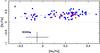 |
Fig. 7 Relation between [Sr/Fe] and [Na/Fe]. The symbols are the same as in Fig. 4. |
| In the text | |
|
Fig. 8 Variation of the lithium abundance in evolved stars in M 4, NGC 6397, and field metal-poor stars as a function of the effective temperature. |
| In the text | |
|
Fig. 9 A(Li) vs. [Na/Fe] for turnoff stars selected in our sample within a very small interval of temperature: 5880 ≤ Teff ≤ 5980 K and computed with A)vt from Monaco et al. (2012), and B) vt = 1.3 km s-1. |
| In the text | |
|
Fig. 10 A(Li) vs. [C/Fe] for turnoff stars selected in our sample within a very small interval of temperature: 5880 ≤ Teff ≤ 5980 K and with A) vt from Monaco et al. (2012) and B) vt = 1.3 km s-1. |
| In the text | |
Current usage metrics show cumulative count of Article Views (full-text article views including HTML views, PDF and ePub downloads, according to the available data) and Abstracts Views on Vision4Press platform.
Data correspond to usage on the plateform after 2015. The current usage metrics is available 48-96 hours after online publication and is updated daily on week days.
Initial download of the metrics may take a while.