| Issue |
A&A
Volume 654, October 2021
|
|
|---|---|---|
| Article Number | A170 | |
| Number of page(s) | 15 | |
| Section | Stellar structure and evolution | |
| DOI | https://doi.org/10.1051/0004-6361/202141288 | |
| Published online | 27 October 2021 | |
The metal-poor end of the Spite plateau
II. Chemical and dynamical investigation⋆,⋆⋆
1
GEPI, Observatoire de Paris, Université PSL, CNRS, 5 Place Jules Janssen, 92190 Meudon, France
e-mail: This email address is being protected from spambots. You need JavaScript enabled to view it.
2
ESO – European Southern Observatory, Alonso de Cordova 3107, Vitacura, Santiago, Chile
3
Indian Institute of Astrophysics, Koramangala II block, Bengaluru, 560034 Karnataka, India
4
Leibniz-Institut für Astrophysik Potsdam, 14482 Potsdam, Germany
5
GEPI, Observatoire de Paris, Université PSL, CNRS, 77 Av. Denfert-Rochereau, 75014 Paris, France
6
UPJV, Université de Picardie Jules Verne, 33 rue St Leu, 80080 Amiens, France
Received:
11
May
2021
Accepted:
22
August
2021
Abstract
Context. The study of old, metal-poor stars deepens our knowledge on the early stages of the universe. In particular, the study of these stars gives us a valuable insight into the masses of the first massive stars and their emission of ionising photons.
Aims. We present a detailed chemical analysis and determination of the kinematic and orbital properties of a sample of 11 dwarf stars. These are metal-poor stars, and a few of them present a low lithium content. We inspected whether the other elements also present anomalies.
Methods. We analysed the high-resolution UVES spectra of a few metal-poor stars using the Turbospectrum code to synthesise spectral lines profiles. This allowed us to derive a detailed chemical analysis of Fe, C, Li, Na, Mg, Al, Si, CaI, CaII, ScII, TiII, Cr, Mn, Co, Ni, Sr, and Ba.
Results. We find excellent coherence with the reference metal-poor First Stars sample. The lithium-poor stars do not present any anomaly of the abundance of the elements other than lithium. Among the Li-poor stars, we show that CS 22882-027 is very probably a blue-straggler. The star CS 30302-145, which has a Li abundance compatible with the plateau, has a very low Si abundance and a high Mn abundance. In many aspects, it is similar to the α-poor star HE 1424-0241, but it is less extreme. It could have been formed in a satellite galaxy and later been accreted by our Galaxy. This hypothesis is also supported by its kinematics.
Key words: stars: abundances / stars: Population II / line: formation / line: profiles / Galaxy: abundances / Galaxy: evolution
The table with equivalent widths discussed in this paper is only available at the CDS via anonymous ftp to cdsarc.u-strasbg.fr (130.79.128.5) or via http://cdsarc.u-strasbg.fr/viz-bin/cat/J/A+A/654/A170
Based on observations collected at the European Organisation for Astronomical Research in the Southern Hemisphere (Programmes 076.A-0463 PI(Lopez), 077.D-0299 PI(Bonifacio)), 086.D-0871(A) (PI Meléndez).
© A. M. Matas Pinto et al. 2021
 Open Access article, published by EDP Sciences, under the terms of the Creative Commons Attribution License (https://creativecommons.org/licenses/by/4.0), which permits unrestricted use, distribution, and reproduction in any medium, provided the original work is properly cited.
1. Introduction
The lithium observed in metal-poor stars is built up during the Big Bang nucleosynthesis (see e.g., Pitrou et al. 2018). It is a very fragile element that is destroyed by proton fusion when the temperature reaches about 2 106 K. In a main-sequence star, this element is destroyed when the convective zone of the atmosphere reaches the layers in which the temperature is higher than its characteristic fusion temperature. However, in the atmosphere of warm metal-poor dwarf stars, the convective zone is not so deep, and the initial lithium abundance is expected to be preserved. We refer to standard Big Bang nucleosynthesis (SBBN) when we assume that the Universe at the time that primordial nucleosynthesis occurred was homogeneous and isotropic, and there were only three light neutrinos. Under these assumptions, the amount of lithium produced is a non-monotonic function of baryonic density, or equivalently, of the baryon-to-photon ratio. The Planck measurements of the baryonic density (Planck Collaboration XIII 2016) imply that the lithium abundance in the Universe after the Big Bang was A(Li) = 2.75 ± 0.02 dex (Pitrou et al. 2018). In warm dwarf stars in the metallicity range −2.9 < [Fe/H] < −1.5, the observed value of the lithium abundance is constant (the so-called Spite plateau, as noted by Spite & Spite 1982b,a) and close to A(Li) = 2.1 dex (Bonifacio et al. 2007). This value is over three times lower than the expected primordial value.
Bonifacio et al. (2007) studied the lithium abundance of a sample of 18 very and extremely metal-poor (VMP and EMP) turnoff stars (−3.5 < [Fe/H] < −2.5). All the stars with a metallicity higher than [Fe/H] = −2.9 had a lithium abundance compatible with the Spite plateau within the measurement uncertainties, but surprisingly, in the 10 stars with ([Fe/H]< − 3.0, the scatter of the Li abundance was large. The Li abundance was sometimes at the level of the plateau, but sometimes significantly below, never above. It was then decided to increase the sample of the metal-poor turnoff stars in order to refute or confirm the behaviour of the lithium abundance at low metallicity. A new sample of 11 metal-poor stars was then studied (Sbordone et al. 2010, hereafter Paper I), the abundances of iron and lithium were computed in this sample, and a meltdown (see Paper I) of the lithium plateau at low metallicity was confirmed (see also e.g., Aoki et al. 2009; Matsuno et al. 2017a; Aguado et al. 2019).
The disagreement between the observed abundance of Li in the stars of the plateau and the abundance predicted by the standard Big Bang is known as the cosmological lithium problem and has recently been addressed by Molaro et al. (2020) and Simpson et al. (2021), for instance.
The aim of this new paper is to study the other problem that might be related to this: the variable decrease in Li abundance at metallicities lower than [Fe/H] ∼ −3. We present here a complete analysis of the abundance of the elements from Li to Ba in the 11 VMP or EMP stars studied in Paper I, and search for any definite correlation between the lithium abundance and the abundance of the other elements in these stars, which could constrain the behaviour of the lithium abundance at extremely low metallicity. We also investigate whether there is any correlation between the kinematic properties of the stars and their Li abundance.
Many of the stars of this sample have already been studied (see Appendix A), but it was important to have a homogeneous study of all the stars of this sample. In this appendix we only report recent analyses based on high-resolution spectra.
2. Observations
The observations of the stars we studied are described in detail in Paper I (see their Table 1). Briefly, observations were performed with the high-resolution spectrograph UVES (Dekker et al. 2000) at the ESO-VLT. The spectra have a resolving power R ≃ 40 000 and were centred at 390 nm (spectral range: 330–451 nm) and 580 nm (spectral range: 479–680 nm). For two stars (BS 17572-100 and HE 1413-1954) that were previously studied in the frame of the HERES program (Christlieb et al. 2004; Barklem et al. 2005) from UVES spectra centred at 437nm (spectral range: 376–497 nm), the blue spectra were centred at 346 nm (spectral range: 320–386 nm). The S/N of the spectra at 400 nm is only about half of the S/N measured at 670 nm (see Table 1 in Paper I) and thus generally does not exceed 50. For two stars, CS 22188-033 and HE 0148-2611, new UVES spectra from the ESO archives, centred at 390 and 580 nm, were also used, increasing the S/N ratio of the mean spectrum. The data were reduced using the standard UVES pipeline with the same procedures as used in Bonifacio et al. (2007).
3. Analysis
3.1. Stellar parameters
In Paper I, the stellar temperature was determined by different methods: photometry, and the profile of the wings of the hydrogen lines by using different theories for the self-broadening of H lines. The surface gravity was derived by enforcing the same Fe abundance from the Fe I and Fe II lines. As usual, the microturbulence (vt) was determined by ensuring that the abundance of iron is independent of the equivalent width of the lines.
In this investigation, we decided to take advantage of the information provided by the Gaia Data Release 2 (Gaia DR2 Gaia Collaboration 2016, 2018; Arenou et al. 2018) to derive the stellar parameters: effective temperature and surface gravity. In this sample of turnoff stars, the precision of the parallaxes is very high, always better than 12% and generally better than 5%, which allows a very good determination of these parameters. For consistency, we used the reddening E(B − V) given in Table 2 of Paper I, deduced from the maps of Schlegel et al. (1998) and corrected as described in Bonifacio et al. (2000). This reddening correction was converted into the Gaia photometric system by adopting the values derived for a G2V star recommended on the PARSEC site1. The Gaia DR2 photometry is provided in Table 1. By using the parallax provided by the Gaia DR2 catalogue and the reddening, we derived the absolute dereddenned G0 magnitude and the dereddenned colour (BP–RP)0. These values were then compared to the PARSEC isochrones (Bressan et al. 2012; Marigo et al. 2017) computed for different ages. Assuming the metallicity reported by Sbordone et al. (2010) for each star, we extracted from the PARSEC data base a grid of isochrones with ages of 9–14 Gyr, with Gaia DR2 colours, computed using the passbands of Evans et al. (2018). We then interpolated for the observed (BP–RP)0 colour and the absolute G magnitude for each age, and selected the age for which this value was closest to the observed absolute G magnitude. At this point, we obtained Teff and log g by interpolating in the isochrone. The Teff and log g values of the stars deduced from this comparison are given in Table 1. In Fig. 1, an example of the fit of the isochrones is given for the star CS 22188–033. We estimate that the uncertainty in Teff does not exceed 100 K and is about 0.3 dex in log g.
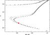 |
Fig. 1. Comparison of the Gaia DR2 photometry of CS 22188-033 to a PARSEC isochrone with a metallicity of −3.0 and age 8, 10, 12, and 14 Gyr. |
Photometric data of the sample, parameters of the atmosphere models, and resulting Fe I and Fe II abundances.
In Fig. 2 we compare our adopted parameters Teff and log g (Table 1) to those adopted in Paper I. The agreement is good within the uncertainties (Δ(Teff) = 8 ± 67 K, Δ(log g) = − 0.17 ± 0.14 dex, where the differences are ours – Paper I). Our log g value is systematically higher by about 0.1 dex than the value adopted in Paper I, however. This may reflect the fact that departures from local thermodynamic equilibrium (LTE) were not taken into account in the calculation of the ionisation equilibrium of Fe in Paper I. Following Thévenin & Idiart (1999), this error may sometimes reach 0.5 dex, in particular, if the low-excitation potential lines of Fe I, which are very sensitive to non-LTE effects, are used for this determination (but this was not the case in Paper I).
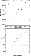 |
Fig. 2. Comparison of the Teff and log g we adopted and the values of the 3D model adopted in Paper I. |
When our microturbulence velocities are compared to the values adopted in Paper I, the differences never exceed 0.2 km s−1. This value corresponds to the uncertainty of the determination.
3.2. Abundance determination
A detailed chemical analysis based on the hypothesis of LTE was performed. MARCS model atmospheres (Gustafsson et al. 1975, 2003; Plez 2008) were used with the code Turbospectrum (Alvarez & Plez 1998; Plez 2012), which computes synthetic spectra to be compared to the observations, allowing us to carry out the study of the element abundances.
When the lines are severely blended or double (e.g., molecular lines or the Li feature), when the damping wings are important (strong Mg lines), or when the lines are affected by hyperfine structure like the Ba II lines, the determination of the abundance was conducted by spectral synthesis. Otherwise, we relied on equivalent width measurements.
The abundances of the elements are given in Table 2. (As usual, for each element X, A(X) = log(N(X)/N(H)) + 12, [X/H] = A(X)−A(X)⊙, and [X/Fe] = [X/H]–[Fe/H].) The iron abundances deduced from the Fe I and Fe II lines are given in Table 1. The value of [Fe/H] in Table 2 is the mean of these values.
Abundance of the elements in the Sun and in our sample of stars.
To calculate [X/Fe], we used the solar abundance values A(X)⊙ provided by Caffau et al. (2011) when available, otherwise we adopted those by Lodders et al. (2009) (see Table 2).
Because our sample of stars has been observed and analysed in almost the same conditions as the stars of the ESO Large Programme “First Stars, first nucleosynthesis” (First Stars, for short), we directly compare our results in the subsequent sections to those of Bonifacio et al. (2009) and Cayrel et al. (2004). However, we must note that the quality of the spectra obtained for these 11 stars is not as good as the quality of the spectra used in Cayrel et al. (2004) and Bonifacio et al. (2007, 2009). The S/N is generally lower than half the S/N obtained for these preceding papers. This parameter is very important in case of very or extremely metal-poor stars, where the lines of many elements are often very weak. In particular, we do not intend to study the star-to-star scatter of the different elements as a function of the metallicity, as was done in the previously cited papers, but only to try to detect some systematic abundance anomalies in the Li-poor stars.
3.3. Abundance uncertainties
Most of the lines of the elements we studied, between C to Ba, are located in the wavelength range 370–550 nm. In this region, the S/N of the spectra is only about half of the S/N obtained in the region of the Li feature (671 nm). As a consequence, the first cause of error for these elements is the uncertainty in the equivalent width (or the profile) of the lines. This uncertainty is generally dominated by the uncertainty in the position of the continuum. In case of weak lines (EW < 10 mA), when the S/N of the spectra is poor, the uncertainty on the equivalent width can be as large as a factor of two, which results in an error 0.3 dex on A(X). This is particularly the case for the lines of HE1413-1954. A second cause of error is the uncertainties in the gf values that are adopted.
The resulting error is estimated as  (where N is for each element X the number of the lines and σ the rms around the mean abundance). In a conservative way, when there are only two lines, an error of 0.15 dex was adopted even if it was σ < 0.15 dex. In case of only one line, we adopted an error of 0.2 dex.
To determine the uncertainties in the abundance determinations A(X) or [X/H], the uncertainties in Teff, log g, and microturbulence vt must be also considered. For these turnoff metal-poor stars, the adopted uncertainties on Teff, log g, and vt are 100 K, 0.3 dex, and 0.2 km s−1 (see Sect. 3.1). Following Bonifacio et al. (2009), these values correspond to an uncertainty on [Fe/H] of about 0.11 dex. We also computed the error on A(Li) due to the uncertainty in the atmospheric parameters (not given in Bonifacio et al. 2009). For turnoff stars, this error is about 0.07 dex, and it is dominated by the error on the effective temperature. The total error on A(X) or [X/H] includes errors linked to the choice of stellar parameters of the model and to observations.
For elements X heavier than Li, the interesting value is the ratio [X/Fe]. For most of the elements, an error on, for example, the temperature of the model induces about the same error on A(Fe) and A(X), and as a consequence, the error on [X/Fe] is small. We have adopted the values given in the Table 4 of Bonifacio et al. (2009), taking into account (linearly) that in our case the adopted error on log g is three times larger.
3.4. Lithium
3.4.1. 1D LTE computation
The lithium analysis was first conducted by spectral synthesis, investigating the Li 670.7 nm resonance doublet. The adopted atomic data for the Li doublet are the same as those used by Bonifacio et al. (2007) and Sbordone et al. (2010); they are based on Asplund et al. (2006). They take into account the hyperfine structure of the lines and also the isotopic components for an assumed solar isotopic ratio. The abundance A(Li), based on one-dimension models with the approximation of local thermodynamical equilibrium (1D-LTE), is given in Col. 3 of Table 3.
Lithium abundances.
3.4.2. 3D NLTE correction
Abundance corrections due to 3D and NLTE effects may be taken into account by using the analytic fitting functions developed by Mott et al. (2020). Using the individual stellar parameters from Table 1, the metallicity [Fe/H] from Table 2, and the 1D-LTE lithium abundance A(Li) from Table 3 as input for their function FFI, we obtain corrections in the range −0.01 ≲ Δ(FFI) ≲ +0.04 (assuming 6Li/7Li = 0). This closely agrees with the corrections for stars on the Spite plateau shown in Fig. 16 of Mott et al. (2020).
Alternatively, we can use fitting function FFIII with the equivalent width EW from Table 3 instead of the 1D LTE Li abundance. With this method, we obtain corrections in the range −0.05 ≲ Δ(FFIII) ≲ −0.03, significantly more negative than the corrections derived from FFI.
This disagreement arises because the treatment of the radiative opacities in the 3D CO5BOLD (Freytag et al. 2012) model atmosphere and the 1D MARCS model differs in its level of detail (CO5BOLD opacity groups versus detailed MARCS opacity sampling). The corrections Δ(FFI) are valid if the difference between A(Li)3D − NLTE − A(Li)1D − LTE is insensitive to the description of the opacities as long as the same treatment is used to construct the 3D and the 1D model. On the other hand, Δ(FFIII) is valid if the EW of the 3D NLTE synthetic line profile is insensitive to small changes in 3D temperature structure related to the description of the radiative opacities.
Comparison of 1D models with different opacity schemes shows that neither of the above conditions is strictly valid (see e.g., Fig. 15 in Mott et al. 2020). A better approximation is to assume that A(Li)3D − NLTE − A(Li)1D − NLTE is invariant under an identical change of the opacities in the 3D and the 1D model. In this case, the abundance correction is given by Δ3 = Δ(FFI , where
  and
and  denote the NLTE corrections computed from 1D models with CO5BOLD and OSMARCS opacities, respectively, but otherwise identical stellar parameters. We find that
  is approximately −0.03, and hence Δ3 ranges between −0.04 and +0.00 for our sample of stars.
We note that the Li abundance corrections for stars on the Spite plateau provided by Wang et al. (2021) appear to be slightly more negative than our Δ(FFI) by about 0.003 dex, judging from their Fig. 11, presumably owing to a different treatment of the UV background opacities in calculating the lithium line formation in statistical equilibrium. Nevertheless, their raw corrections agree almost perfectly with our refined (final) corrections Δ3.
3.4.3. Li abundance
The 3D NLTE Li abundances given in the last column of Table 3 are computed as A(Li)1D − LTE + Δ3.
In Fig. 3 we plot the 3D NLTE Li abundance versus metallicity for our sample of stars (black dots) and for the stars of the First Stars (green dots).
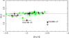 |
Fig. 3. Lithium abundance vs. [Fe/H] for the stars of our sample (black dots) and of the First Stars sample (green dots). The plateau is indicated by a red line. In both samples, the stars that deviate by more than 2σ from the plateau are surrounded by a red circle. |
The observational error is a function of the S/N of the spectrum. We estimated that in this region of the spectrum, it is close to 0.06 dex for S/N = 100 and 0.10 dex for S/N = 70. These estimates are based on the Cayrel formula (Cayrel 1988) and on a direct evaluation of the uncertainty of the best fit of the observed profile because the Cayrel formula does not take the uncertainty in the position of the continuum into account in particular. The estimation of the total error on the Li abundance (quadratic sum of the uncertainty of the model (0.07 dex) and of the observational error) is given in Col. 4 in Table 3. In Fig. 3, several stars deviate significantly from the average. We drew a red circle around the stars whose Li abundance deviates from the average by more than twice the total error given in Col. 4 in Table 3. When these stars are not taken into account, we find that for our sample, the level of the plateau is at A(Li) = 2.14 ± 0.07 and at A(Li) = 2.16 ± 0.07 when we also consider the First Stars sample. The level of this plateau is within the uncertainty compatible with the values found by Bonifacio et al. (2007) (A(Li) = 2.10) and in Paper I (A(Li)3D−NLTE = 2.20). In our sample, only two stars have a Li abundance that deviates from the plateau by more than 2σ: CS 22188-033 and CS 22882-027.
The star CS 22188-033 ([Fe/H] = −2.99) shows a significant lithium depletion (Fig. 3). It confirms a meltdown of the Spite plateau below [Fe/H] = −2.9.
Within the First Stars, three other stars with [Fe/H] < −2.9 were also found with a Li abundance deviating by more than 2 σ from the plateau: CS 22888-031, CS 22948-093, and CS 22966-011 (Bonifacio et al. 2007, and Paper I).
In CS 22882-027, the lithium line is not visible, and it was only possible to derive an upper limit of A(Li). This star is the least metal-poor star of our sample ([Fe/H] = −2.5). In the following, we say for convenience that this star is lithium free. It is discussed in Sect. 5.1.
3.5. Carbon and nitrogen
In this study, C and N abundances were derived from the analysis of molecular bands: for C, the G-band at 425-450 nm formed by CH lines, and for N, the NH band around 336 nm. The parameters of the G-band (Masseron et al. 2014), and the NH band2 were directly taken from the website of Bertrand Plez3.
For all stars in our sample, we analysed the G-band around 430 nm. It is rather weak in these very metal-poor and relatively hot stars, and generally, only an upper limit could be derived. This is provided in Table 2.
The NH band in the near-UV (around 336 nm) is generally outside the spectral range covered by our data. This wavelength range was observed in only two stars: BS 17572-100 and HE 1413-1954. The NH band could be measured in HE 1413-1954, but it is not visible in BS 17572-100 (as is generally the case in turnoff stars).
In our sample, one star, HE 1413-1954, has been reported to be a carbon-enhanced metal-poor (CEMP) star (Masseron et al. 2010; Pols et al. 2012). We confirm the high abundance of C in this hot turnoff star: [C/Fe] = +1.7 dex (Table 2). From the NH band, we found a very high N abundance (A(N) = 7.3, i.e. [N/Fe] = 2.7 dex) in agreement with the literature (see Pols et al. 2012; Lucatello et al. 2006).
In metal-poor stars, the proportion of CEMP stars increases when the metallicity decreases. Following Lucatello et al. (2006), at least 20% of the stars with [Fe/H] < −2.0 are CEMP stars. In these stars, the distribution of the C abundance is bimodally centred around A(C)≃7.0 (low-C band) and A(C)≃8.3 (high-C band) (Bonifacio et al. 2015, 2018). With A(C) = 6.9, HE 1413-1954 belongs to the low-carbon band (see Fig. 2 in Bonifacio et al. 2018).
3.6. α elements magnesium, silicon, calcium, and titanium
3.6.1. Magnesium
Magnesium is produced during hydrostatic phases, specifically, in the burning of carbon in the shells of massive stars. The Mg abundance from the three Mg lines blended by hydrogen lines (around 383 nm) was deduced by spectrum synthesis. The stars of our sample show positive and fairly constant ratios of [Mg/Fe] with values of ⟨[Mg/Fe]⟩ = + 0.24 ± 0.10 dex.
The CEMP star HE 1413-1954 has the highest [Mg/Fe] ratio of our sample. This has been observed for several CEMP stars. The star CS 30302-145 exhibits a significantly low Mg value, [Mg/Fe]= − 0.21, presenting a difference of 0.42 dex from the average value. This star was not taken into account in the computation of the mean [Mg/Fe] ratio. In Figs. 4–7, the position of this star is indicated by a blue square.
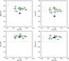 |
Fig. 4. Abundance ratios of the α-elements as a functions of [Fe/H]. The black dots refer to the present study, and the green dots to the First Stars sample. The very lithium-poor stars are surrounded by a pink circle. The α-poor star CS 30302-145 is represented by a blue square. |
3.6.2. Silicon
Silicon is formed during the oxygen burning and in smaller amounts, also by neon burning, in a combination of pre-explosive and explosive phases in type II supernovae (SNe). Abundances of silicon were determined using the line 390.55 nm. The mean value of [Si/Fe] is close to zero. The average value is 0.00 ± 0.22 dex. Following Shi et al. (2009), in the range of temperature and metallicity of the stars we studied, the LTE abundance of Si determined from the 390.55 nm line should be corrected by about +0.25 dex. (This correction was not applied in Table 2).
With [Si/Fe] = −0.49 dex, the star CS 30302-145, which was found to be Mg-poor, is also very Si-poor. (It was not taken into account in the computation of the mean [Si/Fe] ratio.)
3.6.3. Calcium
The Ca lines available in stellar spectra allow to derive A(Ca) in a wide range of metallicity. We took advantage of the investigation of the departure from local thermodynamical equilibrium (NLTE) in Spite et al. (2012) to correct our measurements. The NLTE correction in our stars is about +0.1 dex. The values given in Table 2 are corrected for NLTE effects. Moreover, we did not use the resonance line of neutral calcium at 421.6 nm because in metal-poor stars, the use of this line leads to an underestimation of the Ca abundance, which reaches up to 0.3 dex at [Ca/H] = −3.0 (see e.g., Spite et al. 2012). The mean abundance we found is ⟨[Ca I/Fe]⟩ = + 0.46 ± 0.18 dex.
The abundance of Ca deduced from the ionised lines is based on one single measured line, the Ca II-K line at 392.3 nm. The Ca abundance derived from Ca I and Ca II lines generally agrees well (see Table 2).
However, we note that CS 30302-145 is an exception, and if we had used the abundance of Ca deduced from the Ca II line, this star, poor in Mg and Si, would have the lowest value of [Ca/Fe] of our sample ([Ca/Fe] = 0.2 dex).
3.6.4. Titanium
The theoretical studies of core-collapse SNe and hypernovae predict the ejection of large quantities of titanium (Limongi & Chieffi 2003a,b). The explosion mechanisms have a substantial impact on the production of titanium. The abundance of titanium was derived using the lines of ionised titanium, which is the dominant species in our sample of stars. The titanium-to-iron ratio is very consistent in all the stars of the sample: ⟨[Ti/Fe]⟩ = 0.38 ± 0.17 dex.
3.7. Light odd-Z metals: sodium, aluminium
3.7.1. Sodium
In massive stars, sodium is created mostly during hydrostatic carbon burning and partly during hydrogen burning through the NeNa cycle (see e.g., Cristallo et al. 2009; Romano et al. 2010). Here we studied the sodium D doublet lines (588.99 nm and 589.59 nm), which are the only sodium lines observed in EMP stars. These lines are affected by NLTE effects. In Table 2 we applied the NLTE corrections provided by Andrievsky et al. (2007). In these warm metal-poor turnoff stars, the correction is only about −0.07 dex. The mean value of [Na/Fe] in our sample is ⟨[Na/Fe]⟩ = −0.43 ± 0.22 dex.
The Mg-Si-poor star CS 30302-145 has the lowest sodium abundance ratio [Na/Fe] = −0.90.
3.7.2. Aluminium
In massive stars, aluminium is a product of carbon and neon burning (Limongi & Chieffi 2003a,b; Nomoto et al. 2013). We analysed the resonance doublet of Al I at 394.40 and 396.15 nm. Both lines are sensitive to departure from LTE. We applied the corrections by Andrievsky et al. (2008). In these metal-poor turnoff stars, the NLTE correction is positive and very significant. It increases the LTE Al abundance by about +0.65 dex. The values given in Table 2 are corrected for NLTE. The mean [Al/Fe] value is −0.12 ± 0.10 dex (if we do not take into account CS 30302–145).
The [Al/Fe] value of the Mg-Si-poor star CS 30302–145 is 0.55 dex lower than the average value (see Fig. 5).
3.8. Elements formed during complete and incomplete Si burning
We included the iron peak elements Sc, Cr, Mn, Fe, Co, and Ni. Iron is the most tightly bound nucleus, and the iron peak elements are the last for which fusion reactions are the main mode of production. In the matter that formed the old very metal-poor stars, these elements were ejected by type II SNe, and their production occurs during Si burning in the pre-SN phase and in the explosive phase (Limongi & Chieffi 2003a,b).
3.8.1. Scandium
Scandium is exclusively observed in its singly ionised state. Our scandium abundances were measured using the Sc II line at 424.68 nm. When comparing our results with the First Stars sample (Bonifacio et al. 2009), we have an excellent agreement.
The nucleosynthesis of this element is linked to the mass of the parent stars (Chieffi & Limongi 2002). If the gas out of which these stars were formed had been enriched by a few SNe with slightly different masses, we could expect a high dispersion in scandium abundances, which in our case (Fig. 5) is not observed.
There is one exception: the very lithium-poor star CS 22882–027. This star stands out with the lowest scandium abundance at about 3 σ from the mean.
The chemical evolution models of the Galaxy do not represent the evolution of the abundance of this element well (Kobayashi et al. 2006; Matteucci 2016). They generally underestimate the scandium abundance at low metallicity.
3.8.2. Chromium
The explosive combustion of silicon is the main source of chromium (see e.g., Woosley & Weaver 1995; Chieffi & Limongi 2002; Umeda & Nomoto 2002). Our LTE analysis based on Cr I lines shows the well-known decrease in [Cr/Fe] with decreasing metallicity. Following Bergemann & Cescutti (2010), this is an effect of NLTE on neutral chromium. The NLTE correction is about +0.4 dex at [Fe/H] = −3 and only +0.2 dex at [Fe/H] = −2. If we apply this correction to our sample of stars and to the stars studied in Bonifacio et al. (2009), the ratio [Cr/Fe] is practically constant and close to zero in our metallicity range. The values given in Table 2 are not corrected for NLTE.
3.8.3. Manganese
At low metallicity, manganese is mainly made during silicon burning in core-collapse SNe. Our determination of the abundance of Mn in our sample of turnoff stars is based on the resonance Mn triplet at 403 nm, which is known to be strongly affected by departure from LTE (Bergemann & Gehren 2008; Bergemann et al. 2019). This NLTE correction has not been applied in Table 2 or in Fig. 6. The average value is ⟨[Mn/Fe]⟩ = −0.64. Moreover, in Fig. 6, the most metal-poor stars seem to be more Mn poor, but this can be explained by the strong increase in NLTE correction when the metallicity decreases (see Fig. 9 in Bergemann et al. 2019), but this correction has not been computed below [Fe/H] = −3.
Here again the Mg-Si-poor dwarf CS 30302-145 stands out in the sample. It shows a considerably higher manganese abundance than the remaining sample (see Fig. 6). This latter value has not been taken into account in the computation of the average (its value is 0.56 dex above this average).
3.8.4. Cobalt
In our very metal-poor turnoff stars, the Co abundance is derived from the Co I lines at 384.5, 399.5, and 412.1 nm. These lines are known to be widened by hyperfine splitting structure and are very sensitive to departure from LTE (Bergemann 2008; Bergemann et al. 2010). In our classical LTE analysis, we observe an increase in [Co/Fe] as the stellar metallicity decreases (see Fig. 6), as was noted by McWilliam et al. (1995), Cayrel et al. (2004), and Bergemann et al. (2010), for example. According to Bergemann et al. (2010), the NLTE correction leads to an even stronger increase in [Co/Fe] with decreasing [Fe/H]. Chemical evolution models of the Galaxy fail to explain this behaviour (see e.g., Romano et al. 2010; Matteucci 2016). Bergemann et al. (2010) suggested that compared to the predicted yields, Co is overproduced relative to Fe in short-lived massive stars.
In Fig. 6 the Mg- and Si-poor dwarf CS 30302-145 has the highest [Co/Fe] ratio of our sample.
3.8.5. Nickel
The mean value of the nickel-to-iron ratio is about zero (Fig. 6), ⟨[Ni/Fe]⟩ = 0.04 ± 0.15 dex, in good agreement with the data of Bonifacio et al. (2009).
The two stars CS 30302-145 and HE 1413-1954 have the highest values of the Ni abundance with respect to iron, see Fig. 6. The error on the Ni abundance of the second star is very large, however.
3.9. Neutron-capture elements Sr and Ba
While elements up to iron are formed by nuclear fusion in an exothermic way, for heavier nuclei, fusion reactions become endothermic because Fe nuclei are the most tightly bound. As a consequence, the preferred route for the formation of heavier nuclei is neutron capture (see e.g., Arnould & Goriely 2020; Cowan et al. 2021, and references therein). This capture can occur through two main processes. A very rapid process (main r-process) in violent events such as explosions following the core collapse of massive SNe, the merging of neutron stars or of black holes, jets, gamma ray bursts, etc. A slow process (main s-process) at a rate much lower than the β decay. This occurs at the end of the evolution of relatively low-mass stars in their asymptotic giant branch (AGB) phase. Because these low-mass stars have a long lifetime, they could not enrich the matter that formed the very old metal-poor stars we studied. In our sample of stars, the abundance of the neutron-capture elements mainly reflects the products of the main r-process.
However, the large scatter of [Sr/Ba] for instance for a given [Ba/Fe] suggests that another mechanism is able to enrich the matter in the early Galaxy (e.g., Spite et al. 2014; Cowan et al. 2021). In Fig. 8, the ratio [Sr/Ba] is plotted versus [Ba/Fe] for the stars of the First Stars sample (dwarfs and giants) and our sample of stars. A star can be Sr rich but Ba poor. Contributions of fast-rotating massive stars through a non-standard s-process (Meynet et al. 2006; Frischknecht et al. 2012, 2016), or supermassive AGB through an intermediate i-process (Cowan & Rose 1977) are generally evoked. The contributions of these other processes become relatively high only in Ba-poor stars, where the matter that formed the star has been little enriched in heavy elements by the main r-process.
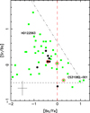 |
Fig. 8. [Sr/Ba] vs. [Ba/Fe]. Green symbols represent the First Stars, circles show dwarfs, and squares show giants. The black dots represent our sample of dwarfs (Ba could be measured in only seven stars of the sample). The three Li-poor dwarf stars (with a measured Ba abundance) are circled in red. The dotted line represents the value [Sr/Ba] provided by the r-process alone. CS 31082-001 is a typical r-rich star, and in contrast, HD 122563, is an r-poor star with a relative enrichment of the first peak elements. |
In warm very metal-poor dwarf stars such as those in our sample, only the abundances of Sr and Ba are measurable in the visible region of the spectrum. In this study, we analysed two ionised strontium lines at 407.7 nm and 421.6 nm and only the Ba line at 493.4 nm because the strongest Ba line at 455.4 nm is generally outside the wavelength range of our spectra: the Ba 455.4 nm line could be measured only in BS 17572-100 and HE 1413-1954.
We could measure the Ba abundance in the C-rich star HE 1413-1954, and we found (Table 2): [Ba/Fe] = 0.01 ± 0.2. This star, which belongs to the low-C band, is as expected not enriched in Ba (see e.g., Fig. 6 in Bonifacio et al. 2015). HE 1413-1954 can be classified as a CEMP-no star (following Beers & Christlieb 2005).
4. Kinematic and orbital properties of the star sample
In this section, we compare the kinematic and orbital parameters of our 11 stars to the First Stars sample that was extensively studied in Di Matteo et al. (2020). In particular, we try to detect, for instance, whether the Li-poor stars (from our sample or the First Stars sample) present any special characteristics.
We used the GalPot code4 (Dehnen & Binney 1998) together with the galactic model of McMillan (2017) to derive the kinematical properties of our sample of stars. In this model, the distance of the Sun from the Galactic centre is R⊙ = 8.21 kpc and the local standard of rest (LSR) velocity, VLSR = 233.1 km s−1 (McMillan 2017). The velocity of the Sun relative to the LSR is U⊙ = 11.1 km s−1, V⊙ = 12.24 km s−1 and W⊙ = 7.25 km s−1 (McMillan 2017). The disc rotates clockwise, and as a consequence, the z-component of the disc angular momentum, Lz, and the disc azimuthal velocity, Vphi, are negative. A star with negative Lz and Vphi is prograde.
The positions, proper motions, and parallaxes of our sample of stars are taken from Gaia DR2, but the radial velocities were measured on the spectra (Table 1 in Paper I) with a precision of 1 km s−1. The sample of stars we studied has about the same distance distribution, between 0.4 and 1.9 kpc (Table 1), as the sample of dwarfs studied in the frame of the First Stars (Di Matteo et al. 2020), which is used here also as a chemical comparison sample. The error on the parallax for all the stars is lower than 12% (see Table 1). The main kinematical data and orbital properties of these stars are presented in Table 4.
Galactic coordinates, velocities, and main orbital parameters of the stars we studied.
− X, Y, Z are the galactic coordinates of the stars, and VX, VY, VZ their velocities in the three directions. X, Y, Z, are given in kpc and the velocities in km s−1.
−  is the distance of the star to the Galactic centre in kpc, and VR is the component of the velocity in this direction: VR = (XVX + YVY)/R.
− Lz, the z component of the angular momentum, is equal to XVY − YVX.
− Lperp, the perpendicular angular momentum component, is equal to  (with Lx = YVZ − ZVY and Ly = ZVX − XVZ). Angular momenta are given in units of 100 kpc km s−1.
− The azimuthal velocity Vphi is defined as the z component of the angular momentum divided by R, that is, Vphi = Lz/R.
− The energy of the orbit is given in units of 100 km2 s−2. In Fig. 9 we compare the position of our stars (black dots) to the position of the First Stars (grey dots) in the five classical diagrams:
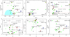 |
Fig. 9. Characteristics of the orbital kinematics. Our stars are represented by black dots, and the dwarfs of the First Stars by green dots. The Li-poor stars are circles in red, the Li-free star by a red square, and the low-α star by a blue square. The other very metal-poor and low-α star HE 1424-0241 (Cohen et al. 2007) is indicated by an open blue diamond. In panel A, the blue zone shows the location of the disc stars in this diagram. In panels C and E, the location occupied mainly by accreted stars is indicated. In panel D, the dotted lines delimit the region in which the Nissen & Schuster (2010) stars are located. Units of the plotted quantities are velocities in km s−1, distances in kpc, angular momenta in 100 kpc km s−1, and energy in 100 km2 s−2. It is important to note that in the zone marked as containing “accreted stars”, e.g., there is only a high probability that the stars in this zone are accreted, and this is the same for the zone marked “in situ”. Exceptions may exist (Schuster et al. 2012). |
– Fig. 9A Toomre diagram, Vphi vs.  ;
;
– Fig. 9B zmax vs. Rmax and arctan(Rmax/zmax) vs. Rmax
– Fig. 9C Lperp vs. Lz
– Fig. 9D eccentricity vs. Lz
– Fig. 9E Energy vs. Lz.
Generally speaking, in Fig. 9 our new set of stars (black dots) occupies the same location as the dwarfs of the First Stars sample (green dots). The Li-poor stars (with A(Li) < 2.0) in our new star sample and in the First Stars sample are circled in red, the Li-free star CS 22882-27 by a red square, and the low-α star CS 30302-145 by a blue square. In the remainder of this paper, we discuss the position of our new sample of stars and of the Li-poor stars from our sample or the First Stars sample.
Haywood et al. (2018) and Di Matteo et al. (2020) showed that the low-α and high-α stars of the Nissen & Schuster (2010) sample and the Gaia DR2-APOGEE sample (Di Matteo et al. 2019) occupy different positions in the diagrams of Fig. 9 (see in particular Fig. 5 in Di Matteo et al. 2020). From these positions, it has been possible to define different zones populated mainly by accreted stars or stars formed in situ. These different zones are reported in Fig. 9. Simulations suggested indeed that the low-α stars in the Nissen & Schuster (2010) and the Gaia DR2-APOGEE samples are the remnants of an accretion event in the early history of the Milky Way. The stars in these samples are more metal rich than the stars of the First Stars sample and the 11 stars we studied, but Di Matteo et al. (2020) showed that despite their different abundance content, they can share the same common origin.
However, we must insist on the fact that there is an important overlap in kinematics properties of the stars. It clearly appears that there is no sharp transition between the accreted stars and the stars formed in situ (in contrast to what might be thought from our Fig. 9). A star in a region noted “accreted stars” in Fig. 9 has only a higher probability to be an accreted star than a star located in a region noted “stars formed in situ”.
The Toomre diagram (see Fig. 9A) shows that, like the First Stars sample, our stars are mainly prograde. The light blue area shows the location of the disc stars. Most of our stars are rather close to this zone. The azimuthal velocity Vphi (and the z component of the angular momentum Lz) of the Li-poor stars is generally close to zero.
Most of the 11 stars we studied remain during their life in or close to the thick disc with zmax ≤ 5 kpc, (see Fig. 9B1). Only HE 0148-2611 and the Li-poor star of the First Stars sample, CS 22948-093, have a zmax value higher than 10 kpc. Two stars with Rmax > 40 kpc are moving far away from the Galactic centre : CS 29514-07 and the Li-poor star of the First Stars sample, CS 22948-93.
Following Di Matteo et al. (2020), the stars with arctan(Rmax/zmax) < 0.2 (see Fig. 9B2) are in a zone in which most of the stars are formed in situ. In the zone where arctan(Rmax/zmax) values are above 0.5, the stars are in contrast probably accreted. (The limits between accreted stars and stars formed in situ are discussed in detail in Sect. 5.3).
One Li-poor star CS22188-33 is in the zone of the “in situ stars”, but another Li-poor star, CS22948-93, is in the zone of the “accreted stars”. The Li-free star CS22882-27 is in the zone of the “accreted stars”.
In Fig. 9C, only one star of our sample (HE 1413-1954) is in the region Lz < −10 kpc km s−1, in which following Di Matteo et al. (2020), most of the stars were formed in situ.
Two stars with Lz > −10 kpc km s−1 associated with Lperp ≳ 13 kpc km s−1, are in a zone only populated by accreted stars, following Di Matteo et al. (2020): HE 0148-2611 and the Li-poor star CS 22948-93. The Li-free star CS22882-27 is at the limit of this zone, which is mostly occupied by the accreted stars.
The region with of Lz > −10 kpc km s−1 but Lperp < 13 kpc km s−1 is the locus in which stars of the Gaia-Sausage-Enceladus structure (GSE, Belokurov et al. 2018; Haywood et al. 2018; Helmi et al. 2018) are redistributed, but also the locus of in-situ stars is heated to halo-like kinematics by accretion (Di Matteo et al. 2019). The α-poor star CS 30302-145 belongs to this mixed region.
In Fig. 9D, the relation between the eccentricity and the angular momentum Lz is presented. The locations of most of the Gaia-DR2-APOGEE and Nissen & Schuster (2010) stars are indicated by dotted lines. The four Li-poor stars have an angular momentum close to zero, and as most of the stars with this Lz value, they have a high eccentricity (ecc > 0.85) (see Di Matteo et al. 2020).
Figure 9E shows the relation between the energy E and the angular momentum Lz. Following Di Matteo et al. (2020), stars with E > −1500 km2 s−2 are most probably accreted because they lie in a region that is populated only by accreted stars in the Gaia-DR2-APOGEE and Nissen & Schuster (2010) samples. In this region, we find three stars of our sample, CS22950-173, HE014826-11, and the α-poor star CS 30302-145. The Li-poor star CS22948-93 also belongs to this “accreted zone”.
The positions of our sample of stars in the different diagrams of Fig. 9 are summarised in Table 5. The Li-free CS22882-027 presents many characteristics of the accreted stars and also the Li-poor star CS22948-093. In contrast, the Li-poor star CS22188-033, with its very low value of arc tang (zmax/Rmax), seems to have been formed in situ. The other Li-poor stars CS22888-031 and CS22966-011 are in zones in which accreted stars and stars formed in situ are found (mixed zones).
Status of the stars of our sample.
We note that the star CS29514-007, with its low value of arctan(Rmax/zmax), seems to have been formed in situ. In contrast, its very high energy value suggests that it has been accreted.
5. Discussion
5.1. Colour-magnitude diagram, age of the stars, and the blue straggler CS 22882-027.
In Fig. 10 we plot the position of the PARSEC metallicity isochrones −3.0 for different ages (see also Sect. 3.1) in a G0 versus (Bp−Rp)0 diagram. The positions of the stars of our sample are marked by black dots, and the two Li-poor stars are circles in red.
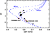 |
Fig. 10. Comparison of PARSEC metallicity isochrones of −3.0 and ages 8, 12, and 14 Gyr with the position of the stars in the colour-magnitude diagram. The colours (Bp−Rp)0 and the G0 magnitudes of the stars have been computed from the Gaia-DR2 photometry. The stars of our sample are represented by black dots, and the Li-poor stars (stars that deviate by more than 2σ from the Li plateau) are circled in red. The three Li-poor stars from the First Stars sample (green dots) have been added. |
All the stars in Fig. 10 are compatible with an age in the range of 12–14 Gyr, as expected from their low metallicity.
However, one star, CS 22882-027, seems to be much younger. According to the isochrone, its age is 8 Gyr and its mass is 0.8 M⊙, slightly higher than the masses estimated for the other stars, which are in the range 0.67–0.78 M⊙. Moreover, we have seen that it has no measurable lithium (Sect. 3.4). These are two characteristics of blue stragglers (Bonifacio et al. 2019). A blue straggler is the result of the merging of two stars. Lithium is destroyed in the merging process, and the newly formed star, which has a higher mass, occupies a position on the colour-magnitude diagram that would normally be populated by genuinely younger stars. Ryan et al. (2001) suggested that the stars with no detectable Li are blue-stragglers-to-be and Bonifacio et al. (2019) showed that three out of four of the stars investigated by Ryan et al. (2001) are indeed canonical blue-stragglers. We note that CS 22882-027 has a normal abundance of all the other elements except for Sc, whose abundance is very low (see Fig. 6).
5.2. Li-poor stars
In addition to the blue straggler CS 22882-027, another star of our sample, CS 22188-033, has a rather low Li abundance, and during the Large Programme First Stars, three other stars were also found with a Li abundance deviating by more than 2 σ from the plateau (see Sect. 3.4). These three stars are plotted in Fig. 10 as green dots. All these lithium-poor stars have a normal distribution of the other elements. They do not present any systematic chemical anomaly.
It is interesting to remark that although we mainly studied stars located at the turnoff, three out of four Li-poor stars (excluding the blue straggler CS 22882-027) are on the main sequence before the turnoff (see Fig. 10). This could suggest that in the most metal-poor dwarfs, some kind of atmospheric phenomenon (possibly diffusion) brings Li in the deep atmosphere, from where it is again mixed in the photosphere as the star reaches the turnoff and the surface convective zone deepens (see also Mucciarelli et al., in prep., priv. comm.).
5.3. Stars: accreted or formed in situ?
The kinematic properties reflect large intrinsic differences between the stars formed in situ and those derived from accretion events. The most massive galaxies have a higher percentage of stellar accretion, and they harbour the most metal-poor stars (Oser et al. 2010; Simon 2019). Table 5 provides the kinematical characteristics of the stars and their probability to be accreted or formed in situ.
However, we must note that all our interpretation is based on the assumption that the high-α stars observed by Nissen & Schuster (2010) (with [Fe/H] ≈ −1.2) mostly have an in-situ origin, and that low-α stars are mostly associated with accretion events (Di Matteo et al. 2020). On the one hand, Renaud et al. (2021) recently showed that a population of high-α stars can also be formed through accretion of massive satellites (see their Fig 8), and on the other hand, Khoperskov et al. (2021) showed that a population of low-metallicity, low-α stars can also be formed in situ in the outer regions of Milky Way-type galaxies, where the star formation efficiency may be low (see some of the cases shown in Fig. 8 of their paper).
On the basis of their orbital properties, and if we assume that our interpretation of the observations of Nissen & Schuster (2010) is correct, we can deduce that six stars of our sample have probably been accreted and that three stars were probably formed in situ (Table. 5).
The star CS 29514–007 presents ambiguous characteristics. It has a low value of arctan(Rmax/zmax), but a high Rmax (Fig. 9). It lies in a region where both accreted and in-situ stars are found. It may be possibly accreted, as suggested also by its high energy value. This interpretation does not contradict the finding of Amarante et al. (2020) and Koppelman et al. (2020), who showed that structures or wedges discussed by Haywood et al. (2018) in the zmax–Rmax plane depend on the different orbital families populated by halo stars and resonant orbits.
5.4. α-poor star CS 30302-145
The EMP star CS 30302-145 we studied has a low abundance of the α elements Mg and Si, but the [Ca/Fe] ratio is consistent with the sample average (see Fig. 4). In this star, the odd light metals Na and Al (see Fig. 5) are also deficient, but it is clearly Mn-rich and belongs to the stars with the highest ratios of [Co/Fe] and [Ni/Fe] (see Fig. 6).
A similar behaviour has been observed in another EMP star, HE 1424-0241, a giant with [Fe/H] ≃ −4 (Cohen et al. 2007). This star also has a very low [Si/Fe] ratio, but in contrast to CS 30302-145, Mg is about normal and Ca is deficient. Both stars are Mn rich. For these two stars, we computed the differences between their value of [X/Fe] and the value of [X/Fe] in similar “normal” stars. For HE 1424-0241, we took the normal giants from the 0Z survey as a reference, evaluated at [Fe/H] = −4 (Cohen et al. 2007, Col. 7), and for CS 30302-145, we adopted the mean value, estimated at [Fe/H] = −3, from Bonifacio et al. (2009). In Fig. 11 we plot this difference as a function of the atomic number. CS 30302-145 is much less extreme than HE 1424-0241.
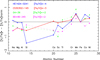 |
Fig. 11. Comparison of the abundances of the α-poor star. The star CS 30302-145 in our sample (red line, whose metallicity is [Fe/H] ∼ −3) compared with the stars in the literature, HE 1424-0241 (blue line, with [Fe/H] ∼ −4, Cohen et al. 2002). Two less metal-poor but α-poor stars BD+80 245 (pink line), and G4-36 (green line) have been added to this figure ([Fe/H] ∼ −2 following Ivans et al. 2003). |
In Fig. 11 we also add (dotted lines) two less metal-poor but α-poor subgiants BD+80 245 and G4-36 (Ivans et al. 2003; Salvadori et al. 2019) with [Fe/H] ≃ −2. For these stars, we adopted as a reference the mean value of [X/Fe] at [Fe/H] = −2.0 following Reggiani et al. (2017). Another α-poor star (and r-process-enhanced star) has been reported by Sakari et al. (2019), this horizontal-branch star with [Fe/H] = −1.9, RAVE J 0937-0626, is also poor in Mg, Al, Si, and Ca, but it does not seem to be enriched in Mn or in Co.
All the stars in Fig. 11 present a similar trend, but the differences from star to star are significant. In BD+80 245 and G4-36, which are less metal-poor ([Fe/H] = −2), Ivans et al. (2003) tried to explain the distribution of the elements as caused by the effect of the first SN Ia. They concluded that the abundance distribution they observed could only be explained by a strong contribution of the SN Ia events. The same explanation was suggested by Sakari et al. (2019) for RAVE J 0937-0626.
This is unlikely to occur in stars as metal-poor as CS 30302-145 or HE 1424-0241. The matter that formed these two stars could be enriched only by the ejecta of SN II, and following Cohen et al. (2007), the different models of SN II yields are not able to explain the peculiar distribution of the elements.
Salvadori et al. (2019) suggested that BD+80 245 ([Fe/H] = −2.0) had been enriched by very massive first stars exploding as pair-instability SNe (PISN). This star has indeed a very low abundance of Zn, a characteristic of the ejecta of PISN. This might be also possible for the matter that formed CS 30302-145. We thus tried to measure the Zn abundance in CS 30302-145 in order to detect a Zn deficiency. We found [Zn/Fe] < + 1, this does not allow us to decide if the star is Zn poor or not. In extremely metal-poor stars, it is in fact impossible to detect a deficiency of Zn with an S/N as low as about 65 around the zinc line at 481 nm.
In CS 30302-145, we were only able to measure the abundance of Sr of the neutron-capture elements. It is highly deficient, but at this metallicity, many normal metal-poor stars are Sr-poor (see e.g., François et al. 2007).
We note that the star CS 30302-145 has a retrograde orbit (see Fig. 9A) and that its energy is relatively high (Fig. 9E). As a consequence, this star may have been formed in a dwarf galaxy and have later been accreted by the Milky Way.
6. Conclusions
The aim of this study was to perform a detailed chemical analysis for a sample of 11 dwarf halo stars that extends from main sequence to turnoff, in order to detect abundance anomalies in Li-poor stars.
A few of these very metal-poor stars ([Fe/H] ≤ −3.0) are indeed characterised by a lower Li abundance than the Spite plateau. We were able to compare the chemical pattern of stars on this plateau to the Li-depleted stars, and we did not find any significant difference.
The star CS 22882-027, in which the lithium line is not visible, seems to be a canonical blue straggler, as suggested by Ryan et al. (2001), and Bonifacio et al. (2019). In this star, the Sc abundance is rather low.
The CEMP star HE 1413-1954 belongs to the low-carbon band, and as expected, it is a CEMP-no (without enrichment in heavy elements, see Bonifacio et al. 2015, 2018). We note that the Li abundance in this star is compatible with the Spite plateau (Masseron et al. 2012; Matsuno et al. 2017b).
The star CS 30302-145 shows low abundances of all the α elements except for Ca, but it has a high value of Mn. A similar behaviour was observed in the α-poor EMP star ([Fe/H] = −4) HE 1424-0241 Cohen et al. (2007), but with some differences.
i/ The odd elements Na and Al are over-deficient in CS 30302-145, but not in HE 1424-0241.
ii/ Unlike in CS 30302-145, Mg is normal in HE 1424-0241 and Ca is deficient.
iii/ The relatively high value of the energy of the orbit of CS 30302-145 might indicate that this star has been accreted, but this is not the case of HE 1424-0241.
The age of all the stars in our sample extends from 12 to 14 Gyr. (One star, CS 22882-027, seems to be younger, but we have shown that it is very likely a blue straggler.)
In the study of the kinematic and orbital properties of the stars, we observed (Table 5) that the parameters of 6 of the 11 stars are compatible to an accretion by our Galaxy. The orbital parameters of only one star, the C-rich star HE 1413-1954, suggest that this star was very probably formed in situ.
The blue straggler CS 22882-027 and the α-poor star CS 30302-145 may have been formed in another galaxy and been accreted later.
Considered collectively, the Li-poor stars do not have any specific orbital characteristics. All have highly eccentric orbits, and they are almost equally divided between prograde and retrograde stars.
http://stev.oapd.inaf.it/cgi-bin/cmd. Using the Cardelli et al. (1989) plus O’Donnell (1994) extinction curves with total-to-selective extinction ratio of 3.1 the following extinction coefficients are derived: AG/AV = 0.85926, ABP/AV = 1.06794, ARP = 0.65199.
Acknowledgments
We gratefully acknowledge support from the French National Research Agency (ANR) funded project “Pristine” (ANR-18-CE31-0017). This work has made use of data from the European Space Agency (ESA) mission Gaia (https://www.cosmos.esa.int/gaia), processed by the Gaia Data Processing and Analysis Consortium (DPAC, https://www.cosmos.esa.int/web/gaia/dpac/consortium). Funding for the DPAC has been provided by national institutions, in particular the institutions participating in the Gaia Multilateral Agreement.
References
- Aguado, D. S., González Hernández, J. I., Allende Prieto, C., et al. 2019, ApJ, 874, L21 [NASA ADS] [CrossRef] [Google Scholar]
- Allen, D. M., Ryan, S. G., Rossi, S., et al. 2012, A&A, 548, A34 [NASA ADS] [CrossRef] [EDP Sciences] [Google Scholar]
- Alvarez, R., & Plez, B. 1998, A&A, 330, 1109 [NASA ADS] [Google Scholar]
- Amarante, J. A. S., Smith, M. C., & Boeche, C. 2020, MNRAS, 492, 3816 [NASA ADS] [CrossRef] [Google Scholar]
- Andrievsky, S. M., Spite, M., Korotin, S. A., et al. 2007, A&A, 464, 1081 [NASA ADS] [CrossRef] [EDP Sciences] [Google Scholar]
- Andrievsky, S. M., Spite, M., Korotin, S. A., et al. 2008, A&A, 481, 481 [NASA ADS] [CrossRef] [EDP Sciences] [Google Scholar]
- Aoki, W., Barklem, P. S., Beers, T. C., et al. 2009, ApJ, 698, 1803 [NASA ADS] [CrossRef] [Google Scholar]
- Arnould, M., & Goriely, S. 2020, Prog. Part. Nucl. Phys., 112, 103766 [NASA ADS] [CrossRef] [Google Scholar]
- Arenou, F., Luri, X., Babusiaux, C., et al. 2018, A&A, 616, A17 [NASA ADS] [CrossRef] [EDP Sciences] [Google Scholar]
- Asplund, M., Lambert, D. L., Nissen, P. E., et al. 2006, ApJ, 644, 229 [Google Scholar]
- Barklem, P. S., Christlieb, N., Beers, T. C., et al. 2005, A&A, 439, 129 [NASA ADS] [CrossRef] [EDP Sciences] [Google Scholar]
- Beers, T. C., & Christlieb, N. 2005, ARA&A, 43, 531 [NASA ADS] [CrossRef] [Google Scholar]
- Belokurov, V., Erkal, D., Evans, N. W., et al. 2018, MNRAS, 478, 611 [NASA ADS] [CrossRef] [Google Scholar]
- Bergemann, M. 2008, Phys. Scr. Vol. T, 133, 014013 [NASA ADS] [CrossRef] [Google Scholar]
- Bergemann, M., & Gehren, T. 2008, A&A, 492, 823 [NASA ADS] [CrossRef] [EDP Sciences] [Google Scholar]
- Bergemann, M., & Cescutti, G. 2010, A&A, 522, A9 [NASA ADS] [CrossRef] [EDP Sciences] [Google Scholar]
- Bergemann, M., Pickering, J. C., & Gehren, T. 2010, MNRAS, 401, 1334 [CrossRef] [Google Scholar]
- Bergemann, M., Gallagher, A. J., Eitner, P., et al. 2019, A&A, 631, A80 [NASA ADS] [CrossRef] [EDP Sciences] [Google Scholar]
- Boehm-Vitense, E. 1981, ARA&A, 19, 295 [NASA ADS] [CrossRef] [Google Scholar]
- Bonifacio, P., Monai, S., & Beers, T. C. 2000, AJ, 120, 2065 [Google Scholar]
- Bonifacio, P., Molaro, P., Sivarani, T., et al. 2007, A&A, 462, 851 [NASA ADS] [CrossRef] [EDP Sciences] [Google Scholar]
- Bonifacio, P., Spite, M., Cayrel, R., et al. 2009, A&A, 501, 519 [NASA ADS] [CrossRef] [EDP Sciences] [Google Scholar]
- Bonifacio, P., Caffau, E., Spite, M., et al. 2015, A&A, 579, A28 [NASA ADS] [CrossRef] [EDP Sciences] [Google Scholar]
- Bonifacio, P., Caffau, E., Spite, M., et al. 2018, A&A, 612, A65 [NASA ADS] [CrossRef] [EDP Sciences] [Google Scholar]
- Bonifacio, P., Caffau, E., Spite, M., et al. 2019, Res. Notes Am. Astron. Soc., 3, 64 [Google Scholar]
- Bressan, A., Marigo, P., Girardi, L., et al. 2012, MNRAS, 427, 127 [NASA ADS] [CrossRef] [Google Scholar]
- Caffau, E., Ludwig, H.-G., Steffen, M., Freytag, B., & Bonifacio, P. 2011, Sol. Phys., 268, 255 [Google Scholar]
- Cardelli, J. A., Clayton, G. C., & Mathis, J. S. 1989, ApJ, 345, 245 [Google Scholar]
- Carretta, E., Gratton, R., Cohen, J. G., et al. 2002, AJ, 124, 481 [NASA ADS] [CrossRef] [Google Scholar]
- Cayrel, R. 1988, The Impact of Very High S/N Spectroscopy on Stellar Physics, 132, 345 [NASA ADS] [CrossRef] [Google Scholar]
- Cayrel, R., Depagne, E., Spite, M., et al. 2004, A&A, 416, 1117 [NASA ADS] [CrossRef] [EDP Sciences] [Google Scholar]
- Chieffi, A., & Limongi, M. 2002, ApJ, 577, 281 [NASA ADS] [CrossRef] [Google Scholar]
- Christlieb, N., Beers, T. C., Barklem, P. S., et al. 2004, A&A, 428, 1027 [NASA ADS] [CrossRef] [EDP Sciences] [Google Scholar]
- Cohen, J. G., Christlieb, N., Beers, T. C., et al. 2002, AJ, 124, 470 [NASA ADS] [CrossRef] [Google Scholar]
- Cohen, J. G., McWilliam, A., Christlieb, N., et al. 2007, ApJ, 659, L161 [NASA ADS] [CrossRef] [Google Scholar]
- Cowan, J. J., & Rose, W. K. 1977, ApJ, 212, 149 [Google Scholar]
- Cowan, J. J., Sneden, C., Lawler, J. E., et al. 2021, Rev. Mod. Phys., 93, 015002 [Google Scholar]
- Cristallo, S., Straniero, O., Gallino, R., et al. 2009, ApJ, 696, 797 [NASA ADS] [CrossRef] [Google Scholar]
- Dehnen, W., & Binney, J. 1998, MNRAS, 294, 429 [Google Scholar]
- Dekker, H., D’Odorico, S., Kaufer, A., et al. 2000, Proc. SPIE, 534 [NASA ADS] [CrossRef] [Google Scholar]
- Di Matteo, P., Haywood, M., Lehnert, M. D., et al. 2019, A&A, 632, A4 [NASA ADS] [CrossRef] [EDP Sciences] [Google Scholar]
- Di Matteo, P., Spite, M., Haywood, M., et al. 2020, A&A, 636, A115 [NASA ADS] [CrossRef] [EDP Sciences] [Google Scholar]
- Evans, D. W., Riello, M., De Angeli, F., et al. 2018, A&A, 616, A4 [NASA ADS] [CrossRef] [EDP Sciences] [Google Scholar]
- Freytag, B., Steffen, M., Ludwig, H.-G., et al. 2012, J. Comput. Phys., 231, 919 [Google Scholar]
- Frischknecht, U., Hirschi, R., & Thielemann, F.-K. 2012, A&A, 538, L2 [NASA ADS] [CrossRef] [EDP Sciences] [Google Scholar]
- Frischknecht, U., Hirschi, R., Pignatari, M., et al. 2016, MNRAS, 456, 1803 [Google Scholar]
- François, P., Depagne, E., Hill, V., et al. 2007, A&A, 476, 935 [Google Scholar]
- Gaia Collaboration (Prusti, T., et al.) 2016, A&A, 595, A1 [NASA ADS] [CrossRef] [EDP Sciences] [Google Scholar]
- Gaia Collaboration (Brown, A. G. A., et al.) 2018, A&A, 616, A1 [NASA ADS] [CrossRef] [EDP Sciences] [Google Scholar]
- Gustafsson, B., Bell, R. A., Eriksson, K., & Nordlund, Å. 1975, A&A, 42, 407 [Google Scholar]
- Gustafsson, B., Edvardsson, B., Eriksson, K., et al. 2003, in Stellar Atmosphere Modeling, eds. I. Hubeny, D. Mihalas, K. Werner, et al., ASP Conf. Ser., 288, 331 [NASA ADS] [Google Scholar]
- Haywood, M., Di Matteo, P., Lehnert, M. D., et al. 2018, ApJ, 863, 113 [Google Scholar]
- Helmi, A., Babusiaux, C., Koppelman, H. H., et al. 2018, Nature, 563, 85 [Google Scholar]
- Ivans, I. I., Sneden, C., James, C. R., et al. 2003, ApJ, 592, 906 [NASA ADS] [CrossRef] [Google Scholar]
- Khoperskov, S., Haywood, M., Snaith, O., et al. 2021, MNRAS, 501, 5176 [NASA ADS] [CrossRef] [Google Scholar]
- Kobayashi, C., Umeda, H., Nomoto, K., et al. 2006, ApJ, 653, 1145 [NASA ADS] [CrossRef] [Google Scholar]
- Koppelman, H. H., Bos, R. O. Y., & Helmi, A. 2020, A&A, 642, L18 [NASA ADS] [CrossRef] [EDP Sciences] [Google Scholar]
- Limongi, M., & Chieffi, A. 2003a, Mem. Soc. Astron. It. Suppl., 3, 58, http://sait.oats.inaf.it/MSAIS/3/POST/Limongi_talk.pdf [Google Scholar]
- Limongi, M., & Chieffi, A. 2003b, http://sait.oats.inaf.it/MSAIS/3/POST/Limongi_talk.pdf [Google Scholar]
- Lodders, K., Palme, H., & Gail, H. P. 2009, Landolt Börnstein, 712 [Google Scholar]
- Lucatello, S., Beers, T. C., Christlieb, N., et al. 2006, ApJ, 652, L37 [NASA ADS] [CrossRef] [Google Scholar]
- Marigo, P., Girardi, L., Bressan, A., et al. 2017, ApJ, 835, 77 [Google Scholar]
- Masseron, T., Johnson, J. A., Plez, B., et al. 2010, A&A, 509, A93 [NASA ADS] [CrossRef] [EDP Sciences] [Google Scholar]
- Masseron, T., Johnson, J. A., Lucatello, S., et al. 2012, ApJ, 751, 14 [NASA ADS] [CrossRef] [Google Scholar]
- Masseron, T., Plez, B., Van Eck, S., et al. 2014, A&A, 571, A47 [NASA ADS] [CrossRef] [EDP Sciences] [Google Scholar]
- Matsuno, T., Aoki, W., Beers, T. C., et al. 2017a, AJ, 154, 52 [NASA ADS] [CrossRef] [Google Scholar]
- Matsuno, T., Aoki, W., Suda, T., et al. 2017b, PASJ, 69, 24 [NASA ADS] [CrossRef] [Google Scholar]
- Matteucci, F. 2016, J. Phys. Conf. Ser., 703, 012004 [NASA ADS] [CrossRef] [Google Scholar]
- McMillan, P. J. 2017, MNRAS, 465, 76 [NASA ADS] [CrossRef] [Google Scholar]
- McWilliam, A., Preston, G. W., Sneden, C., et al. 1995, AJ, 109, 2757 [NASA ADS] [CrossRef] [Google Scholar]
- Meléndez, J., Casagrande, L., Ramírez, I., et al. 2010, A&A, 515, L3 [NASA ADS] [CrossRef] [EDP Sciences] [Google Scholar]
- Meyer, B. S. 1994, ARA&A, 32, 153 [NASA ADS] [CrossRef] [Google Scholar]
- Meynet, G., Ekström, S., & Maeder, A. 2006, A&A, 447, 623 [NASA ADS] [CrossRef] [EDP Sciences] [Google Scholar]
- Molaro, P., Cescutti, G., & Fu, X. 2020, MNRAS, 496, 2902 [Google Scholar]
- Mott, A., Steffen, M., Caffau, E., et al. 2020, A&A, 638, A58 [NASA ADS] [CrossRef] [EDP Sciences] [Google Scholar]
- Nissen, P. E., & Schuster, W. J. 2010, A&A, 511, L10 [NASA ADS] [CrossRef] [EDP Sciences] [Google Scholar]
- Nomoto, K., Kobayashi, C., & Tominaga, N. 2013, ARA&A, 51, 457 [CrossRef] [Google Scholar]
- O’Donnell, J. E. 1994, ApJ, 422, 158 [Google Scholar]
- Oser, L., Ostriker, J. P., Naab, T., et al. 2010, ApJ, 725, 2312 [NASA ADS] [CrossRef] [Google Scholar]
- Pitrou, C., Coc, A., Uzan, J.-P., et al. 2018, Phys. Rep., 754, 1 [NASA ADS] [CrossRef] [Google Scholar]
- Planck Collaboration XIII. 2016, A&A, 594, A13 [NASA ADS] [CrossRef] [EDP Sciences] [Google Scholar]
- Plez, B. 2008, Phys. Scr. Vol. T, 133, 014003 [NASA ADS] [CrossRef] [Google Scholar]
- Plez, B. 2012, Astrophysics Source Code Library [record ascl:1205.004] [Google Scholar]
- Pols, O. R., Izzard, R. G., Stancliffe, R. J., et al. 2012, A&A, 547, A76 [NASA ADS] [CrossRef] [EDP Sciences] [Google Scholar]
- Preston, G. W., & Sneden, C. 2000, AJ, 120, 1014 [Google Scholar]
- Reggiani, H., Meléndez, J., Kobayashi, C., et al. 2017, A&A, 608, A46 [NASA ADS] [CrossRef] [EDP Sciences] [Google Scholar]
- Renaud, F., Agertz, O., Read, J. I., et al. 2021, MNRAS, 503, 5846 [NASA ADS] [CrossRef] [Google Scholar]
- Roederer, I. U., Preston, G. W., Thompson, I. B., et al. 2014, AJ, 147, 136 [Google Scholar]
- Romano, D., Karakas, A. I., Tosi, M., et al. 2010, A&A, 522, A32 [NASA ADS] [CrossRef] [EDP Sciences] [Google Scholar]
- Ryan, S. G., Beers, T. C., Kajino, T., et al. 2001, ApJ, 547, 231 [NASA ADS] [CrossRef] [Google Scholar]
- Sakari, C. M., Roederer, I. U., Placco, V. M., et al. 2019, ApJ, 874, 148 [NASA ADS] [CrossRef] [Google Scholar]
- Salvadori, S., Bonifacio, P., Caffau, E., et al. 2019, MNRAS, 487, 4261 [NASA ADS] [CrossRef] [Google Scholar]
- Sbordone, L., Bonifacio, P., Caffau, E., et al. 2010, A&A, 522, A26 (Paper I) [NASA ADS] [CrossRef] [EDP Sciences] [Google Scholar]
- Shi, J. R., Gehren, T., Mashonkina, L., et al. 2009, A&A, 503, 533 [NASA ADS] [CrossRef] [EDP Sciences] [Google Scholar]
- Schlegel, D. J., Finkbeiner, D. P., & Davis, M. 1998, ApJ, 500, 525 [Google Scholar]
- Schuster, W. J., Moreno, E., Nissen, P. E., et al. 2012, A&A, 538, A21 [NASA ADS] [CrossRef] [EDP Sciences] [Google Scholar]
- Simon, J. D. 2019, ARA&A, 57, 375 [NASA ADS] [CrossRef] [Google Scholar]
- Simpson, J. D., Martell, S. L., Buder, S., et al. 2021, MNRAS, 507, 43 [NASA ADS] [CrossRef] [Google Scholar]
- Spite, F., & Spite, M. 1982a, A&A, 115, 357 [NASA ADS] [Google Scholar]
- Spite, M., & Spite, F. 1982b, Nature, 297, 483 [NASA ADS] [CrossRef] [Google Scholar]
- Spite, M., Cayrel, R., Hill, V., et al. 2006, A&A, 455, 291 [NASA ADS] [CrossRef] [EDP Sciences] [Google Scholar]
- Spite, M., Andrievsky, S. M., Spite, F., et al. 2012, A&A, 541, A143 [NASA ADS] [CrossRef] [EDP Sciences] [Google Scholar]
- Spite, M., Spite, F., Bonifacio, P., et al. 2014, A&A, 571, A40 [NASA ADS] [CrossRef] [EDP Sciences] [Google Scholar]
- Suda, T., Yamada, S., Katsuta, Y., et al. 2011, MNRAS, 412, 843 [NASA ADS] [Google Scholar]
- Thévenin, F., & Idiart, T. P. 1999, ApJ, 521, 753 [CrossRef] [Google Scholar]
- Tinsley, B. M. 1979, ApJ, 229, 1046 [Google Scholar]
- Umeda, H., & Nomoto, K. 2002, ApJ, 565, 385 [Google Scholar]
- Wallerstein, G. 1962, ApJS, 6, 407 [NASA ADS] [CrossRef] [Google Scholar]
- Wang, E. X., Nordlander, T., Asplund, M., et al. 2021, MNRAS, 500, 2159 [Google Scholar]
- Woosley, S. E., & Weaver, T. A. 1995, ApJS, 101, 181 [Google Scholar]
- Zhang, L., Karlsson, T., Christlieb, N., et al. 2011, A&A, 528, A92 [NASA ADS] [CrossRef] [EDP Sciences] [Google Scholar]
Appendix A: Comparison with the recent literature
-
BS 17572-100 (or HE 0926-0508): This star has been studied by Barklem et al. (2005) in the frame of the ESO-Hambourg survey, and Meléndez et al. (2010) determined its Li abundance. Zhang et al. (2011) determined the abundance of Si in this star, taking the NLTE effects into account. When we consider that our value of A(Si) has to be increased by 0.25 for NLTE correction and that the log gf value adopted by Zhang et al. (2011) is 0.05 lower than our value (from Vald3), the agreement between our determinations and theirs is very good (A(Si)NLTE = 4.94 and 5.01, rectively).
-
CS 22950-173: This is one of the blue metal-poor stars for which Preston & Sneden (2000) searched for a variation in radial velocity. They concluded that it was not a spectroscopic binary. They found a metallicity [Fe/H] 0.2 dex higher than our value, but this is explained by the fact that they adopted a temperature (based on the old relation B − V color versus Teff, following Boehm-Vitense (1981)) almost 500 K higher than ours. Spite et al. (2014) also found a metallicity slightly higher than ours, but this is also due to an adopted higher temperature, which in this case was based on the profile of the Hα wings. Moreover, in both cases, the Fe lines list is not exactly the same.
-
CS 29514-007: This star is considered a CEMP-no star in the extensive study of EMP stars carried out by Roederer et al. (2014). We obtained the same metallicity as Roederer et al. (2014) for this star, but they found A(C) = 6.49 while we were only able to estimate an upper limit of the carbon abundance: A(C) ≤ 6.33. We do not have a clear explanation for this difference in the A(C) determination. It might be that the G-band is so weak that the C determination is uncertain in any case. Unfortunately, unlike ESO, Magellan does not have a public archive, so we were unable to directly compare the UVES spectrum we analysed with that of Mike. In any case, this star is not a true CEMP star according to the Beers & Christlieb (2005) definition: metal-poor star with [C/Fe]> +1.
-
HE 0148-2611: This star was studied by Carretta et al. (2002) from HIRES Keck spectra. With about the same atmospheric parameters (Cohen et al. 2002) as those we deduced from the Gaia photometry, they obtained a lower metallicity [Fe/H]=–3.5 instead of [Fe/H]=–3.2 (Table 2).
-
HE 1413-1954: This star is classified as a CEMP star following Masseron et al. (2010) and Suda et al. (2011). Our values agree fairly well with those of Masseron et al. (2010). Our higher value of the [C/Fe] ratio can be explained by the large uncertainty of the C abundance due to to the low S/N of the spectrum in the region of the CH band. This star was also analysed by Allen et al. (2012), and their abundances agree with our determinations. The C abundance determination by Zhang et al. (2011) for this star perfectly agrees with our value. They also computed an NLTE profile of the Si 3905 line, however, and their A(Si) value was found to be much higher than ours. If we apply a NLTE correction (+0.25 dex following Shi et al. 2009) to our value, we find A(Si)NLTE = 4.25, to be compared to the value A(Si)NLTE = 5.04, after correcting the log gf value by 0.05 (see BS 17572-100 at the beginning of this section). These values are not compatible, although the same ESO-UVES spectra were used. The slight difference in the adopted effective temperature cannot explain this effect. In Fig A.1, we show the fit of our profile of the Si line.
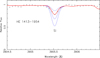 |
Fig. A.1. LTE profile of the Si line in HE 1413-1954 computed with A(Si) = 3.7, 4.3, and 4.8 (blue lines) and with the best-fit value A(Si) = 4.01 (red line). The NLTE value of A(Si) = 5.09 would in this figure correspond to an LTE A(Si) value of about 4.8, which is incompatible with the observed profile, |
All Tables
Photometric data of the sample, parameters of the atmosphere models, and resulting Fe I and Fe II abundances.
Galactic coordinates, velocities, and main orbital parameters of the stars we studied.
All Figures
|
Fig. 1. Comparison of the Gaia DR2 photometry of CS 22188-033 to a PARSEC isochrone with a metallicity of −3.0 and age 8, 10, 12, and 14 Gyr. |
| In the text | |
|
Fig. 2. Comparison of the Teff and log g we adopted and the values of the 3D model adopted in Paper I. |
| In the text | |
|
Fig. 3. Lithium abundance vs. [Fe/H] for the stars of our sample (black dots) and of the First Stars sample (green dots). The plateau is indicated by a red line. In both samples, the stars that deviate by more than 2σ from the plateau are surrounded by a red circle. |
| In the text | |
|
Fig. 4. Abundance ratios of the α-elements as a functions of [Fe/H]. The black dots refer to the present study, and the green dots to the First Stars sample. The very lithium-poor stars are surrounded by a pink circle. The α-poor star CS 30302-145 is represented by a blue square. |
| In the text | |
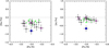 |
Fig. 5. Odd element abundance. Symbols are the same as in Fig. 4. |
| In the text | |
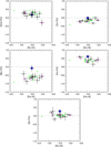 |
Fig. 6. Iron peak elements. Symbols are the same as in Fig. 4. |
| In the text | |
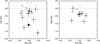 |
Fig. 7. Neutron-capture elements. Symbols are the same as in Fig. 4. |
| In the text | |
|
Fig. 8. [Sr/Ba] vs. [Ba/Fe]. Green symbols represent the First Stars, circles show dwarfs, and squares show giants. The black dots represent our sample of dwarfs (Ba could be measured in only seven stars of the sample). The three Li-poor dwarf stars (with a measured Ba abundance) are circled in red. The dotted line represents the value [Sr/Ba] provided by the r-process alone. CS 31082-001 is a typical r-rich star, and in contrast, HD 122563, is an r-poor star with a relative enrichment of the first peak elements. |
| In the text | |
|
Fig. 9. Characteristics of the orbital kinematics. Our stars are represented by black dots, and the dwarfs of the First Stars by green dots. The Li-poor stars are circles in red, the Li-free star by a red square, and the low-α star by a blue square. The other very metal-poor and low-α star HE 1424-0241 (Cohen et al. 2007) is indicated by an open blue diamond. In panel A, the blue zone shows the location of the disc stars in this diagram. In panels C and E, the location occupied mainly by accreted stars is indicated. In panel D, the dotted lines delimit the region in which the Nissen & Schuster (2010) stars are located. Units of the plotted quantities are velocities in km s−1, distances in kpc, angular momenta in 100 kpc km s−1, and energy in 100 km2 s−2. It is important to note that in the zone marked as containing “accreted stars”, e.g., there is only a high probability that the stars in this zone are accreted, and this is the same for the zone marked “in situ”. Exceptions may exist (Schuster et al. 2012). |
| In the text | |
|
Fig. 10. Comparison of PARSEC metallicity isochrones of −3.0 and ages 8, 12, and 14 Gyr with the position of the stars in the colour-magnitude diagram. The colours (Bp−Rp)0 and the G0 magnitudes of the stars have been computed from the Gaia-DR2 photometry. The stars of our sample are represented by black dots, and the Li-poor stars (stars that deviate by more than 2σ from the Li plateau) are circled in red. The three Li-poor stars from the First Stars sample (green dots) have been added. |
| In the text | |
|
Fig. 11. Comparison of the abundances of the α-poor star. The star CS 30302-145 in our sample (red line, whose metallicity is [Fe/H] ∼ −3) compared with the stars in the literature, HE 1424-0241 (blue line, with [Fe/H] ∼ −4, Cohen et al. 2002). Two less metal-poor but α-poor stars BD+80 245 (pink line), and G4-36 (green line) have been added to this figure ([Fe/H] ∼ −2 following Ivans et al. 2003). |
| In the text | |
|
Fig. A.1. LTE profile of the Si line in HE 1413-1954 computed with A(Si) = 3.7, 4.3, and 4.8 (blue lines) and with the best-fit value A(Si) = 4.01 (red line). The NLTE value of A(Si) = 5.09 would in this figure correspond to an LTE A(Si) value of about 4.8, which is incompatible with the observed profile, |
| In the text | |
Current usage metrics show cumulative count of Article Views (full-text article views including HTML views, PDF and ePub downloads, according to the available data) and Abstracts Views on Vision4Press platform.
Data correspond to usage on the plateform after 2015. The current usage metrics is available 48-96 hours after online publication and is updated daily on week days.
Initial download of the metrics may take a while.