| Issue |
A&A
Volume 667, November 2022
|
|
|---|---|---|
| Article Number | A139 | |
| Number of page(s) | 11 | |
| Section | Galactic structure, stellar clusters and populations | |
| DOI | https://doi.org/10.1051/0004-6361/202243960 | |
| Published online | 18 November 2022 | |
Detailed analysis of a sample of field metal-poor N-rich dwarfs⋆
GEPI, Observatoire de Paris, PSL Research University, CNRS, Place Jules Janssen, 92190 Meudon, France
e-mail: This email address is being protected from spambots. You need JavaScript enabled to view it.
Received:
5
May
2022
Accepted:
13
September
2022
Abstract
Aims. The aim of this work is to compare the detailed chemical composition of the field N-rich dwarf stars to the second-generation stars of globular clusters (GCs) in order to investigate the hypothesis that they originated in GCs.Methods. We measured the abundance of 23 elements (from Li to Eu) in a sample of six metal-poor N-rich stars (three of them pointed out for the first time), and we compared their chemical composition to (i) the chemical composition observed in a sample of classic metal-poor stars and (ii) the abundances observed in the second-generation stars of GCs.Results. In metal-poor N-rich stars, C and O are slightly deficient, but the scatter of [(C+N+O)/Fe] is very small, a strong indication that the N enrichment is the result of pollution by CNO-processed material. The N-rich stars of our sample, similarly to the second-generation stars in the GCs, show an excess of Na and sometimes of Al, as expected if the material from which these stars were formed, has been polluted by the ejecta of massive asymptotic giant branch (AGB) stars. For the first time, we have been able to establish an anti-correlation Na–O in field stars such as the one observed in NGC 6752. The N-rich star HD 74000 has a rather low [Eu/Ba] ratio for its metallicity. Such an anomaly is also observed in several second-generation stars of M 15.Conclusions. This analysis supports the hypothesis that the N-rich stars observed today in the field were born as second-generation stars in GCs.
Key words: stars: abundances / Galaxy: abundances / globular clusters: general / molecular data
Based on observations collected at the European Organisation for Astronomical Research in the Southern Hemisphere (archives of programmes 090.B-0504(A) PI Chaname; 095.D-0504(A) PI Melendez; 076.B-0166(A) PI Pasquini; 067.D-0086(A) PI Gehren; 071.B-0529(A) PI Silva; 065.L-0507(A) PI Primas), and collected at the W. M. Keck Observatory, archive programme G401H, PI Melendez. One star was also observed at ESO with the spectrograph ESPRESSO, programme 107.22RU.001 PI Spite, and two stars were observed at the Observatoire de Haute-Provence (archives of programme 10A.PNPS.HALB, PI Halbwachs) and at the Narval spectrograph of the Observatoire du Pic du Midi, programme L172N04, PI Spite.
Deceased on 2021.07.21, https://www.observatoiredeparis.psl.eu/disparition-de-francois-spite.html?lang=en
© M. Spite et al. 2022
 Open Access article, published by EDP Sciences, under the terms of the Creative Commons Attribution License (https://creativecommons.org/licenses/by/4.0), which permits unrestricted use, distribution, and reproduction in any medium, provided the original work is properly cited.
This article is published in open access under the Subscribe-to-Open model. This email address is being protected from spambots. You need JavaScript enabled to view it. to support open access publication.
1. Introduction
It is well known that most globular clusters (GCs) host multiple populations identified by their different chemical compositions. Compared to the first population, the second population is enriched in He, N, and Na and depleted in C and O (Bastian & Lardo 2018; Mucciarelli et al. 2019; Gratton et al. 2019).
To date, there is no complete consensus on the origin of these multiple populations. Generally, the second population of stars is supposed to be the result of a pollution by the ejecta of first-generation stars (see Bastian & Lardo 2018): intermediate mass asymptotic giant branch (AGB) stars (3 < M < 9 M⊙), fast rotating massive stars (FRMS) with M > 15 M⊙ (Maeder & Meynet 2006), and even very massive stars (VMS) with M ∼ 104 M⊙ (Denissenkov & Hartwick 2014).
Gieles & Charbonnel (2020) recently proposed that a very massive star with a mass of M > 1000 M⊙ forms via stellar collisions, during GC formation, and pollutes the intra-cluster medium. Precise determinations of the chemical composition of the first and second populations have been obtained (see, for example, Pasquini et al. 2005, 2007, 2008; Lind et al. 2009), and anti-correlation between the abundance of N, Na, and C, O has been found to be nearly universal among old and massive clusters (Gratton et al. 2019).
Thanks to the Gaia parallaxes and proper motions, we now have direct evidence of stellar streams formed by stars lost by GCs (Ibata et al. 2021). Some GCs also show extended tidal tails. In some cases, like C-19, the narrow metallicity dispersion and sizeable dispersion in Na abundances implies that a stream results from the disruption of a GC, although the cluster, as such, no longer exists (Martin et al. 2022; Yuan et al. 2022). Prior to the availability of the Gaia data, the identification of stars lost from GCs had to rely on their chemical properties.
Large systematic studies were undertaken to find field stars, presenting the same chemical anomalies as those observed in globular clusters (see e.g., Martell et al. 2011; Ramírez et al. 2012). More recently, N-rich metal-poor field giants have been discovered in the Galactic bulge thanks to the large spectroscopic survey APOGEE (Schiavon et al. 2017) and also in the field of our Galaxy with LAMOST (Tang et al. 2020) and APOGEE (Fernández-Trincado et al. 2022). Their analysis suggests that the origin of these stars is indeed related to the disintegration of GCs. However, such an origin is discussed in Bekki (2019), which suggests that N-rich stars in the bulge and in the halo can be formed from the destruction of high-density building blocks where nitrogen-rich stars are formed from an interstellar medium heavily polluted by AGB ejecta.
In the Galaxy, at least, three classes of metal-poor N-rich stars may be found. These are the following: i) the metal-poor giant stars after the bump undergo a deep mixing which brings the CNO-processed material to the surface (Gratton et al. 2000; Spite et al. 2005, 2006) and the stars appear to be C-poor and N-rich; ii) at low metallicity, many stars, dwarfs, and giants are N-rich and C-rich. Following Lucatello et al. (2006), more than 20% of the metal-poor stars with [Fe/H] ≤ −2.0 belong to this class of carbon-enhanced metal-poor (CEMP) stars. The peculiar chemical composition of these stars, rich in C and in N, and often also in neutron-captured elements, is generally explained by pollution from different kinds of AGB stars during the life of the observed stars or by a formation from a material ejected by rotating massive stars (e.g., Masseron et al. 2010; Hansen et al. 2016a,b; Choplin et al. 2016, 2017). Another possibility, invoked in particular to explain the CEMP stars not enriched in neutron-capture elements (CEMP-no), is an enrichment of the cloud that formed the star by faint supernovae, providing only carbon and the lighter elements (Ishigaki et al. 2014; Bonifacio et al. 2015); iii) a third class of stars, the one we are interested in in the present work, contains N-rich stars with a normal C abundance. This type of star seems to exist among field dwarf and giant stars. It is of particular interest to detect dwarf stars belonging to this class, since their atmosphere has not undergone any mixing with CNO-processed material of the deep layers. It is then safer to compare their chemical composition to the chemical composition of dwarfs in GCs.
In metal-poor giant stars, the nitrogen abundance can be measured in the visible or in the red from the CN bands (Schiavon et al. 2017; Tang et al. 2020), but in metal-poor dwarfs the lines of these bands are too weak and only the vibrational band of NH in the near UV (336 nm) can be used (see e.g., Israelian et al. 2004). As a consequence, very few N-rich metal-poor dwarfs have been detected so far. As far as we know, only five metal-poor dwarfs with [Fe/H] ≤ −1.0 have been reported to have a ratio of [N/Fe] > 0.6: HD 25329, HD 74000, HD 97916, HD 160617, and HD 166913 by, in particular, Harmer & Pagel (1973), Schuster (1981), Laird (1985), and Carbon et al. (1986; see also Spite & Spite 1986).
In the present paper, we analyse these five stars suspected (or already known) to be N-rich in detail, and we report the existence of three more metal-poor dwarfs strongly enriched in nitrogen ([N/Fe] ≥ 1.0). In most of these stars, we were able to measure the abundance of the elements extended from Li to Eu and compare the abundance pattern of the elements with the abundance pattern of normal metal-poor stars and of the second-generation stars in GCs.
2. Star sample and reduction
Near-UV spectra of metal-poor dwarf stars around 336 nm have been retrieved from the ESO-VLT-UVES and Keck-HIRES archives. These spectra have often been obtained with the aim of studying the behaviour of Be in these stars and the parameters of their model are, at least in a first approximation, already known. Among these stars, we visually selected three new dwarfs or turnoff stars presenting a very strong NH band: G24-3, G53-41, and G90-3. Following Ramírez et al. (2012), G53-41 is oxygen-poor and Na-rich, key signatures of the abundance anomalies observed in GCs, and thus it was already suspected to have been born in a GC.
Finally, a sample of eight metal-poor dwarfs has been selected, the five stars already known or suspected to be N-rich and three new stars selected for their strong NH band in high resolution spectra.
The characteristics of all the spectra used in this analysis are given in Table 1. All these spectra have a resolving power of R ≥ 40 000 and a signal to noise (S/N) in the region of the NH band larger than 100.
Spectral ranges (in nm) of the spectra used in this study.
2.1. Model parameters and ages
We took advantage of the information provided by the Gaia DR2 (Gaia Collaboration 2018; Arenou et al. 2018) to derive new stellar parameters: effective temperature and surface gravity. We used the distance-dependent reddening provided by Stilism1 (Lallement et al. 2019) to deduce the absolute magnitude G0 and the colours (BP − RP)0 of the stars. We then compared these values to PARSEC isochrones2 (Bressan et al. 2012; Marigo et al. 2017) and we derived Teff, log g, and the age of the star. The data are given in Table 2, and an example of the isochrones is shown in Fig. 1. The distance of the stars has been computed by a simple inversion of the parallax after correcting by the zero-point offset of 0.03 (Lindegren et al. 2018). Since the stars are close, the error on the distance of the star is always less than 3 pc, the error on G0 less than 0.06, and the error on (BP − RP)0 less than 0.03. We finally estimate that the error on Teff is less than 100 K and the error on log g less than 0.2 dex. The age of all the stars is between 12 and 14 Gyr (Table 2), with two exceptions. Firstly, we were not able measure the age of HD 25329 because it is a rather cool star and still on the main sequence; however, from a Bayesian estimation Pace (2013) reported an age of about 5 Gyr for this star (known to have a strong chromospheric activity), which is surprising for a star with a metallicity lower than [Fe/H] = –1.7. Secondly, the age of HD 97916 ([Fe/H] = –0.75) also seems close to 5 Gyr (Table 2). These two stars are discussed hereafter.
Gaia DR2 data, photometry, and model parameters of the stars.
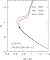 |
Fig. 1. Position of G53-41 (black dot) in a G vs. BP − RP diagram, compared to PARSEC isochrones computed for 10, 12, and 14 Gyr. |
2.2. Chemical composition of the stars
We carried out a classical LTE analysis of the stars using MARCS model atmospheres (Gustafsson et al. 1975, 2003; Plez 2008) and the turbospectrum spectral synthesis code (Alvarez & Plez 1998; Plez 2012). The microturbulence velocity was derived from the Fe I lines, requiring that the abundance derived for individual lines be independent of the equivalent width of the line. The abundances of the elements and [Fe/H] are given in Table 3. We note that we initially selected N-rich stars with [Fe/H] < −1.0, but with the new determination of the atmosphere parameters, HD 97916 was found to be less metal-poor ([Fe/H] = −0.75]). However we decided to keep this star in our sample.
Abundance of the elements.
2.2.1. Atomic data and NLTE corrections
The atomic data were mainly taken from the Vienna Atomic Line Database (VALD3)3. For Ba and Eu the isotopic and hyperfine structure of the lines has been taken into account.
In these dwarf stars, the NLTE effects are generally rather weak, and since the aim of this work is to compare the relative abundances in N-rich dwarfs to those in normal stars with very similar models, these effects were only taken into account for O I, Na I, and Al I.
In this type of star, the oxygen abundance can be generally determined from the red oxygen permitted triplet at 777 nm. Following Zhao et al. (2016) when −2.5 ≤ [Fe/H] ≤ −1.0, the NLTE correction is small and close to about –0.1 dex. This correction was applied in Table 3.
Our determination of the Na abundance is based on the secondary Na I lines at 5682, 5688, 6154, and 6160 Å. The NLTE correction was estimated from Lind et al. (2011). In all our stars it is very close to −0.1 dex, and this correction was applied in Table 3.
To determine the Al abundance, we had to use the resonance lines of Al I. The NLTE correction was computed by Nordlander & Lind (2017) for different atmospheric models. For the turnoff stars, the correction is large, (about +0.4 dex), and it was applied in Table 3.
2.2.2. Molecular data
The carbon abundance was determined from the CH band at 314.4 nm and between 430 and 432.5 nm. The abundances deduced from these two regions are in excellent agreement. The parameters of the CH molecular bands (Masseron et al. 2014) were taken directly from the Bertrand Plez site4.
The nitrogen abundance was derived from the NH band around 336 nm. Spite et al. (2006) showed that the nitrogen abundance based on the Kurucz data is, on average, 0.4 dex higher than the nitrogen abundance deduced from the CN band. At that time, since the data of the CN band seemed more robust, a correction of −0.4 dex was applied to the abundance deduced from the NH band. A similar correction was also used in the determination of the nitrogen abundance in GCs (Pasquini et al. 2008).
More recently, Fernando et al. (2018) presented a new line list of the A3Π−X3Σ− electronic transition of NH based on high-level calculations. This new line list seems to correct this effect (see Sect. 3.3 in Fernando et al. 2018) and has been adopted to compute the N abundance in our stars. The difference between the N abundance measured from the Fernando et al. (2018) line list and the Kurucz line list is 0.50 dex in the 3357–3365 Å region. However, it can be seen in Fig. 2 that the difference is a little smaller around 3364 Å (0.44 dex) and a little larger (0.52 dex) around 3359 Å.
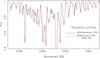 |
Fig. 2. Fit of theoretical NH band computed from the Fernando et al. (2018) data (black line) with A(N)=7.05 and the parameters of HD 74000, with synthetic spectra computed from Kurucz data. The best fit in the total interval 3357–3365 Å is obtained with A(N)=7.55 (red line). In this region, the mean difference of the N abundance computed with these two different sets of data is thus 0.50. |
In Fig. 3, we present the fit of the observed spectrum with synthetic profiles computed with the NH data of Fernando et al. (2018) for the eight stars suspected to be N-rich. In this sample, two stars (HD 97916 and HD 166913) with [N/H] ≤ [Fe/H] are not N-rich stars.
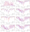 |
Fig. 3. Fit of NH band in our sample of stars known or suspected to be N-rich. The small black crosses are the observed spectrum. The red line represents the best fit of the observed spectrum, and the blue lines show synthetic spectra computed with two different values of A(N) indicated on the figure. For HD 25329, the cooler dwarf of our sample, the region between 3358 and 3362 Å is saturated, and thus we fitted the observed spectra between 3366 and 3369 Å. The values of [Fe/H] and [N/H] are indicated for each star in the figure. |
One of our stars, HD 160617, has already been extensively studied by Roederer & Lawler (2012) in order to determine the abundance distribution of the r-process elements in this star. They used a very similar model atmosphere, and, as expected, there is a good agreement between their abundance determinations and those given in Table 3, with one exception: the abundance of nitrogen. While Roederer & Lawler (2012) found A(N) = 6.61, we measured A(N) = 7.08. The difference is very probably due to the NH line list used by Roederer & Lawler (2012).
The adopted oxygen abundance has been determined as the mean of the abundance deduced from the oxygen triplet of O I (when these lines are not out of the extent of our spectra; see Table 1) and of the abundance deduced from the OH band around 313 nm (Rich & Boesgaard 2009) or 330 nm. As for the CH band, the parameters of the OH band were directly retrieved from the Bertrand Plez site; they are based on the Kurucz line list.
2.3. Comparison of the chemical composition of the NH-rich dwarfs and the normal metal-poor dwarf
To better estimate the peculiarities of the NH-rich stars, we first compared their chemical composition to the composition of normal turnoff metal-poor stars with about the same atmospheric parameters (temperature, gravity, and metallicity). We chose from the paper of Peterson et al. (2020) a sample of metal-poor turnoff stars studied with the same method as described in Sect. 2.2. The parameters of their models and their chemical abundances are given in Table 4. These stars were mainly observed with UVES. For HD 19445, a complementary spectrum was obtained with the spectrograph NARVAL at the Observatoire du Pic du Midi. For HD 140283, the abundances given by Siqueira-Mello et al. (2015) were adopted. We only added the N and O abundances measured from the NH and OH bands on UVES spectra.
Parameters of the model adopted for the comparison stars and abundances of the elements relative to iron.
2.3.1. Nitrogen abundance
In Fig. 4, we present the [N/Fe] ratio as a function of [Fe/H] in the normal field turnoff stars (black dots) and in the eight stars suspected to be N-rich. Among these eight stars, six indeed have a very high abundance of nitrogen with a ratio of [N/Fe] > 1.0 dex (Table 3); they are represented by red squares in Fig. 4. However, two of them, HD 97916 and HD 166913, suspected to be N-rich by Laird (1985), have a normal N abundance with [N/Fe] ≤ 0.0 (blue dots surrounded by red squares in Fig. 4). In Table 3, these two stars are at the end of the list of stars. They are considered as ‘normal’ turnoff stars in the following discussion and represented by blue dots in the subsequent figures.
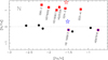 |
Fig. 4. [N/Fe] vs. [Fe/H] for stars studied in the present paper. Red filled square: N-rich stars. Blue dots surrounded by a red square: stars reported as being N-rich from low-resolution spectra and finally found to have a normal nitrogen abundance. Black dots: normal, metal-poor turnoff stars. The blue and red open star symbols represent two dwarf stars in NGC 6752 discussed in Sect. 3. |
From Fig. 4, it could be deduced that a gap exists between the N-rich stars with [N/Fe] > +1.0 and the normal metal-poor stars with [N/Fe] close to zero. In fact, since we visually chose turnoff stars with a very strong NH band, there is a strong bias in our selection. Only a large systematic study of the abundance of nitrogen in field metal-poor turnoff stars could allow us to know if all the N-rich stars have a [N/Fe] ratio close to +1.0 or if there is continuity.
2.3.2. Abundance of the light elements Li Be
In Fig. 5, we compare the lithium and beryllium abundance A(Li) and A(Be) in normal metal-poor dwarfs and in the NH-rich dwarfs. With the temperature scale adopted, based on the Gaia photometry and the PARSEC isochrones, no clear systematic difference between the N-rich stars and the normal turnoff stars is visible. This result is, on a more extended sample, in agreement with the result of Spite & Spite (1986). We note that HD 25329 has no detectable Li, but the temperature of this star is only 4870 K, thus, the convective zone in the atmosphere is deep and Li is brought to hot layers where it is destroyed little by little. This star is not plotted in Fig. 5.
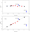 |
Fig. 5. A(Li) and A(Be) vs. [Fe/H] in the stars studied in the present paper. Red squares: N-rich stars. Blue dots: stars reported as being N-rich (from low resolution spectra) and finally found to have a normal nitrogen abundance, black dots normal stars. |
In addition, we note that in the ‘normal’ star, HD 97916, Li is not detected and it is very Be-poor. We derived A(Be) < −0.7, and Boesgaard (2007) measured A(Be) < −1.3 and considered that it is a blue straggler. The fact that we found a very young age for this star (Sect. 2.1) reinforces this interpretation. Moreover, we note that the ‘normal’ star, HD 166913 ([Fe/H) = −1.5), has a high Li abundance: A(Li) = 2.46 (see Fig. 5, upper panel). The Be abundance is also rather high in this star (Fig. 5, lower panel). The 6Li/7Li ratio estimated from the UVES spectrum could be close to 0.1, but the resolution of the spectrum (R = 40 000 in the region of the Li feature) is not sufficient to be confident in this result. An ESPRESSO spectrum of this star (R = 150 000) was recently obtained and is under study. If confirmed, these anomalies (rather high values of Li and Be and presence of 6Li) could be explained by the engulfment of a planet.
2.3.3. Abundance of the elements from C to O
In the −2.5 < [Fe/H] − 0.5 interval, the [C/Fe] and [O/Fe] ratios increase when the metallicity decreases (see Fig. 6), but the C and O abundances in N-rich stars are systematically lower by about 0.3 dex than the abundances in the comparison stars (see Fig. 7). The N-rich stars have practically the same [(C+N+O)/Fe] value as the normal stars. This suggests that the nitrogen in N-rich stars was largely formed at the expense of C and O.
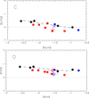 |
Fig. 6. [C/Fe] and [O/Fe] vs. [Fe/H] in the stars studied in the present paper. The symbols are the same as in Fig. 5. The blue star symbol represents NGC 6752-4428 a first-generation dwarf in NGC 6752, and the red star symbol NGC 6752-200613 is a second-generation dwarf (see Sect. 3). |
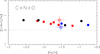 |
Fig. 7. [(C+N+O)/Fe] in our sample of stars. The symbols are the same as in Fig. 6. The [(C+N+O)/Fe] ratio is about the same in normal and N-rich stars. |
2.3.4. Abundance of the odd elements: Na and Al
In Fig. 8, we compare the abundance of Na and Al in N-rich stars and in normal metal-poor stars. We observe that [Na/Fe] is systematically higher in the N-rich stars. It seems that there is also an overabundance of Al in some of these stars, and it reaches almost 0.4 dex in G90-3. Zhao et al. (2016) already noted the high Na abundance in HD 74000 and G90-03 and the high Al abundance in G90-03.
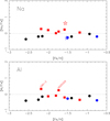 |
Fig. 8. [Na/Fe] and [Al/Fe] vs. [Fe/H] in the stars studied in the present paper. The symbols are the same as in Fig. 6. |
2.3.5. α and iron-peak elements
In nitrogen-rich stars, as in ‘normal’ metal-poor stars, the α elements Mg, Si, Ca, and Ti are enhanced by about 0.4 dex (Fig. 9). The iron-peak elements also behave as they do in normal stars; Cr and Ni have solar [X/Fe] ratios as well as Zn, [Co/Fe] is close to +0.2 dex, and [Mn/Fe] is sub-solar (≃−0.2 dex).
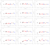 |
Fig. 9. [X/Fe] vs. [Fe/H] for the α elements (Mg to Ti), the iron peak elements (Cr to Zn) and the neutron capture elements (Sr to Eu). The symbols are the same as in Fig. 5. |
2.3.6. Heavy elements
The elements heavier than Zn are formed by the addition of neutrons to iron-peak elements. There are two basic mechanisms able to capture neutrons on existing seed nuclei; firstly, rapid relative to the average β decay (‘r’-process), happens in core-collapse supernovae or during the merging of neutron stars; another one, which is much slower (‘s’-process), happens in thermally pulsing asymptotic giant branch (AGB) stars.
In metal-poor stars, formation by the r-process dominates and the influence of the ‘s’-process appears only for [Fe/H] ≥ −1.4 dex (Roederer et al. 2010). For these heavy elements, the ratio [X/Fe] is more scattered than it is for the α or the iron-peak elements (see e.g., François et al. 2007); this large scatter is observed in Fig. 9, in particular for Ba and Eu. It is well known that some metal-poor stars are rich in Eu and Ba (r-rich stars), and others are Eu and Ba-poor (r-poor stars). HD 140283, the most metal-poor ‘normal’ star in Fig. 9, with [Fe/H] ≃ −2.6, is a classic ‘r-poor’ metal-poor star with a very low abundance of Ba and Eu. At the same metallicity ([Fe/H] ≃ −2.6), many ‘normal’ stars have a higher [Ba/Fe] ratio (see Fig. 10 in François et al. 2007).
In Fig. 10 (upper panel), we have plotted [Zr/Y] as a function of [Fe/H]. There is a rather good correlation of the abundance of Zr and Y in the normal stars of our sample, but there is some indication of a slightly lower ratio of [Zr/Y] in the N-rich stars. However, this difference has to be confirmed by a homogeneous study of larger samples.
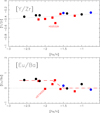 |
Fig. 10. [Zr/Y] and [Eu/Ba] vs. [Fe/H] in the stars studied in the present paper. The symbols are the same as in Fig. 5. |
In the most metal-poor stars, it has been shown that the [Eu/Ba] ratio is close to 0.5 dex (see e.g., François et al. 2007; Spite & Spite 2014; Mashonkina et al. 2010). This is also observed in the most metal-poor stars of our sample (Fig. 10, lower panel) with the exception of the N-rich star HD 74000, which has a solar [Eu/Ba] abundance ratio, despite its low metallicity ([Fe/H] = −2). This is discussed later in Sect. 3.5. When [Fe/H] > −1.5, [Eu/Ba] tends to be solar, as expected following Roederer et al. (2010).
3. Comparison of the abundances in the N-rich stars and in the second-generation stars of the GCs
It is now generally accepted that, inside a GC, first- and second-generation stars cohabit (see e.g., Prantzos et al. 2007; Charbonnel et al. 2014). The second-generation stars were formed from an intracluster gas polluted by H-processed material ejected by a first generation of massive stars. Different objects have been suggested as polluters: mainly fast rotating massive stars (FRMS) with a mass larger than 25 M⊙, massive AGB stars with 6 < M < 11 M⊙, and also massive binaries. The nature of the polluter depends on the initial mass of the GC. Compared to the first generation of stars, the second generation is low in Li, C, and O, but rich in N, Na (Carretta et al. 2005; Pasquini et al. 2005, 2007, 2008; Lind et al. 2009), and sometimes Al (Mészáros et al. 2020; Schiappacasse-Ulloa et al. 2022).
If the six N-rich stars studied here were born in GCs, they certainly do not come from the same cluster, and since the chemical anomalies depend on the mass of the cluster, we do not expect a perfect agreement between our sample of stars and the relations observed in a given GC. These field N-rich stars have different metallicities (from −1.2 dex to −2.2 dex), but they have almost the same value of [N/Fe] (i.e., 1.02 ≤ [N/Fe] ≤ 1.34), and thus any correlation between [N/Fe] and the other elements cannot be firmly established. However, it is interesting to check wether the values observed for Li, C, O, Na, and Al in these stars are comparable to the values in the GCs.
3.1. Comparison of the C, N, and O abundances
We would like to compare the C, N, and O abundance in our N-rich stars with these abundances in second-generation dwarfs of a GC. The nitrogen abundance has been measured from the NH band in two dwarf stars of NGC 6752: NGC 6752-4428 and NGC 6752-200613 by Pasquini et al. (2008). Carretta et al. (2005) measured the N abundance in nine NGC 6752 dwarfs from the CN band including the two stars observed by Pasquini et al. (2008). There is a rather good agreement for the nitrogen abundance in NGC 6752-200613 ([N/Fe] = +1.7 and +1.5), but a clear disagreement for NGC 6752-4428 ([N/Fe] = +1.1 and +0.3). Since in metal-poor dwarfs it is easier to measure the nitrogen abundance from the NH band, we adopted the Pasquini et al. (2008) values, and, in a first step, we did not take into account the nitrogen abundances computed by Carretta et al. (2005).
The star NGC 6752-200613 is strongly enriched in nitrogen ([N/Fe] = 1.5) and Carretta et al. (2005) measured the carbon abundance ([C/Fe] = −0.2 dex), but they could not measure the oxygen abundance from the red oxygen triplet. We tried to measure the oxygen abundance from the OH band in the near UV spectrum used by Pasquini et al. (2007) to measure Be in this star. We obtained [O/Fe] = +0.5 ± 0.3 (the uncertainty is large due to the low S/N in this region of the spectrum). We can thus compare the C, N, and O abundances in NGC 6752-200613 and in the stars of our sample. This is done in Figs. 4, 6, and 7. NGC 6752-200613 is more N-rich than the stars in our sample of N-rich field stars, but the general behaviour of these stars are similar.
In three stars of our N-rich sample, we were able to estimate the 12C/13C ratio (Fig. 11); we found a ratio of 12C/13C ≤ 15, indicating a pollution by CNO-processed material.
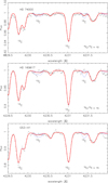 |
Fig. 11. 12C/13C in three of our sample of stars. The computations have been done for 12C/13C = 30 12C/13C = 5 (blue lines) and for the best fit (red line): 12C/13C = 10 for HD 74000 and 12C/13C = 15 for HD 160617 and G53-41. |
3.2. Anti-correlation Na-O
The main characteristic of the GC stars is the anti-correlation between the abundance of Na and the abundance of O (see e.g., Charbonnel et al. 2014). In Fig. 12, we present the [Na/Fe] vs. [O/Fe] relation for our sample of stars. We overplotted the position of the giant stars of NGC6752 following Bastian & Lardo (2018), and that of the dwarf stars following Carretta et al. (2005). The abundance of oxygen in dwarfs is estimated from the O I triplet; the lines are weak, and a precise estimation requires a high S/N. As a consequence, the error in the determination of the oxygen abundance in the dwarfs of NGC 6752 is large. We estimate that it is at least 0.2 dex, and even 0.3 dex in particular for NGC 6752-200613. The general trend of our sample of stars agrees with the trend of the NGC 6752 stars.
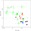 |
Fig. 12. Position of our stars in [Na/Fe] vs. [O/Fe] diagram compared to stars of GC NGC 6752. The symbols are the same as in Fig. 5, the giants in NGC 6752 are represented by small star symbols, and the dwarfs are represented by larger star symbols. The error is larger in the case of dwarfs since they are fainter, and an approximative estimation of this error is indicated in the figure. |
This is the first time that the existence of an Na–O anti-correlation has been demonstrated among field stars. This has been possible because the N-rich stars of our sample proved to be Na-rich and O-poor. This clearly indicates that they are second-generation GC stars. The corollary of this finding is that the first generation of GC stars have a chemical composition that is indistinguishable from that of field stars.
3.3. Anti-correlation Li–Na
A strong anti-correlation between Li and Na has been observed in NGC 6752 (Pasquini et al. 2005), but the slope of this anti-correlation is much weaker in M 4 (Monaco et al. 2012; Spite et al. 2016) and in NGC 6397 (González Hernández et al. 2009; Lind et al. 2009). As a consequence, and since we never observe a very high excess of Na in our metal-poor N-rich stars, we do not expect to observe a clear Li–Na anti-correlation, as it can be guessed from Fig. 5 where N-rich and normal reference stars seem to share the same Li abundance.
3.4. Anti-correlation Al–Mg
In some GCs, an anti-correlation Al–Mg is observed (Mészáros et al. 2020; Baeza et al. 2022, and references therein). The Mg–Al cycle needs large temperatures (> 70 million Kelvin) to operate, but Al-rich stars (with [Al/Fe] > 0.3) are sometimes observed in massive GCs. G 90-3 could be one of these stars. Compared to the other stars, G 90-3 is not Mg-poor, but since there is almost ten times more Mg than Al in the gas, the aluminium abundance is more sensitive to a pollution than Mg.
3.5. Neutron-capture elements in N-rich stars and in the GCs: The [Eu/Ba] ratio
The heavy elements have been studied in detail in very few GCs and only in giant stars. However, since the abundance of these elements in the atmosphere is not expected to vary during the evolution of a star, at least during the main-sequence and red-giant-branch (RGB) phases, it is possible to compare the abundances of the heavy elements in dwarfs and in RGB stars.
In metal-poor GCs (as in very metal-poor stars), r-process production dominates, and the [Eu/Ba] ratio is generally close to 0.5 dex as observed in the very metal-poor field stars. This value is characteristic of the ‘r’-process (see e.g., François et al. 2007; Spite & Spite 2014).
In a given cluster, the abundance of the n-capture elements does not tend to vary from star to star (see e.g., Roederer 2011; Kirby et al. 2020). However, a small number of GCs show variations; the best example of this phenomenon is M 15 (Sobeck et al. 2011; Worley et al. 2013). In this cluster, [Eu/Fe] and [Ba/Fe] vary, and no correlation was established between [Na/Fe] and [Eu/Fe] or [Ba/Fe]. The large scatter of these abundances is attributed to an inhomogeneity of the original cloud.
In this cluster, Johnson & Bolte (2002) found that the [Y/Zr] ratio is lower than in the field stars. From Fig. 10 (upper panel), it also seems that [Y/Zr] is lower in the N-rich stars than in the normal stars. However, the difference is not as large as that (0.3 dex) reported by Johnson & Bolte (2002).
Although [Eu/Fe] varies from star to star, in most of the M 15 stars the ratio [Eu/Ba] is constant, close to the ‘r’-process ratio (+0.5 dex). On the other hand, we remark that in this cluster, following the data of Worley et al. (2013), there are two stars in their ‘S97’ sample with a low [Eu/Ba] ratio (high [Ba/Eu]): K969 and K479 (Fig. 13a in Worley et al. 2013). These stars also have a rather high value of the Na abundance with [Na/Fe] ≥ 0.5 dex (Sneden et al. 1997). Likewise, the star ID42262 in the ‘W13’ sample with a very low [Eu/Ba] ratio (Fig. 13b in Worley et al. 2013) has the highest [Na/Fe] ratio of the sample ([Na/Fe] = +0.9 dex). As a consequence, it seems that in GC stars, a high value of [Na/Fe] is sometimes (not always) associated with a low value of [Eu/Ba], indicating ‘s’-process contamination.
One of our N-rich stars, HD 74000, with [Eu/Ba] = −0.05 at [Fe/H] = −2.0, seems to have a solar [Eu/Ba] ratio that is unexpected for its metallicity (see Fig. 10). This star, similarly to some Na-rich stars in M 15, has probably been polluted by ‘s’-process material ejected by a first-generation AGB stars.
4. Conclusion
We studied a sample of eight dwarf stars suspected to be N-rich (and not enhanced in C), similar to the second-generation stars of GCs. The N abundance is deduced from the computation of the NH band in the near UV, based on the new parameters of Fernando et al. (2018). Two stars suspected to be N-rich by Laird (1985), were found to have a normal N abundance. The other six stars were found to have a ratio of [N/Fe] > 1.0 dex. If the N-rich stars in the field are second-generation stars ejected from GCs, we do not expect the same homogeneity of their chemical composition as found in a given GC, since these stars were formed in different clusters with different initial masses and thus different histories and metal-enrichment.
The abundances of C, N, and O in our sample of N-rich stars present the same characteristics as those found in the second-generation stars of the GCs. C and O are slightly deficient, but the scatter of [(C+N+O)/Fe] is very small. When [Fe/H] decreases from −0.5 to −2.0 dex, [(C+N+O)/Fe] increases from about 0.2 to 0.6 dex as observed in normal stars. This is a strong indication that the N enrichment is the result of pollution by CNO-processed material.
The N-rich stars of our sample, such as the second-generation stars in the GCs, show an excess of Na and sometimes of Al, as expected if these stars have been polluted by the ejecta of AGB stars. An Na–O anti-correlation is observed, similar to the relation observed in NGC 6752.
The N-rich star HD 74000 has a solar value of the ratio [Eu/Ba]; this low value is unexpected for its metallicity ([Fe/H] = −2.0 dex). At this metallicity, the neutron-capture elements are generally only formed by the ‘r’-process and [Eu/Ba] = +0.5 dex. We show that this peculiarity is also observed in at least three stars of M 15, which all have an excess of the Na abundance, as expected for second-generation stars. We suppose that in these stars a first-generation of AGB stars has enriched the matter in ‘s’-process material.
This analysis supports the hypothesis that the N-rich stars observed in the field today were formed as second-generation stars in GCs and lost through the tidal interaction between the GC and the Galaxy.
Acknowledgments
This work uses results from the European Space Agency (ESA) space mission Gaia. Gaia data are being processed by the Gaia Data Processing and Analysis Consortium (DPAC). Funding for the DPAC is provided by national institutions, in particular the institutions participating in the Gaia MultiLateral Agreement (MLA). The Gaia mission website is https://www.cosmos.esa.int/gaia. The Gaia archive website is https://archives.esac.esa.int/gaia.
References
- Alvarez, R., & Plez, B. 1998, A&A, 330, 1109 [NASA ADS] [Google Scholar]
- Andrievsky, S. M., Spite, M., Korotin, S. A., et al. 2008, A&A, 481, 481 [NASA ADS] [CrossRef] [EDP Sciences] [Google Scholar]
- Arenou, F., Luri, X., Babusiaux, C., et al. 2018, A&A, 616, A17 [NASA ADS] [CrossRef] [EDP Sciences] [Google Scholar]
- Baeza, I., Fernández-Trincado, J. G., Villanova, S., et al. 2022, A&A, 662, A47 [NASA ADS] [CrossRef] [EDP Sciences] [Google Scholar]
- Bastian, N., & Lardo, C. 2018, ARA&A, 56, 83 [Google Scholar]
- Bekki, K. 2019, MNRAS, 490, 4007 [Google Scholar]
- Boesgaard, A. M. 2007, ApJ, 667, 1196 [NASA ADS] [CrossRef] [Google Scholar]
- Bonifacio, P., Caffau, E., Spite, M., et al. 2015, A&A, 579, A28 [NASA ADS] [CrossRef] [EDP Sciences] [Google Scholar]
- Bressan, A., Marigo, P., Girardi, L., et al. 2012, MNRAS, 427, 127 [NASA ADS] [CrossRef] [Google Scholar]
- Carbon, D. F., Kraft, R. P., Barbuy, B., et al. 1986, Rev. Mex. Astron. Astrofis., 12, 173 [Google Scholar]
- Carretta, E., Gratton, R. G., Lucatello, S., et al. 2005, A&A, 433, 597 [NASA ADS] [CrossRef] [EDP Sciences] [Google Scholar]
- Charbonnel, C., Chantereau, W., Krause, M., et al. 2014, A&A, 569, L6 [NASA ADS] [CrossRef] [EDP Sciences] [Google Scholar]
- Choplin, A., Maeder, A., Meynet, G., et al. 2016, A&A, 593, A36 [NASA ADS] [CrossRef] [EDP Sciences] [Google Scholar]
- Choplin, A., Hirschi, R., Meynet, G., et al. 2017, A&A, 607, L3 [NASA ADS] [CrossRef] [EDP Sciences] [Google Scholar]
- Denissenkov, P. A., & Hartwick, F. D. A. 2014, MNRAS, 437, L21 [Google Scholar]
- Fernández-Trincado, J. G., Beers, T. C., Barbuy, B., et al. 2022, A&A, 663, A126 [NASA ADS] [CrossRef] [EDP Sciences] [Google Scholar]
- Fernando, A. M., Bernath, P. F., Hodges, J. N., et al. 2018, J. Quant. Spectr. Rad. Transf., 217, 29 [NASA ADS] [CrossRef] [Google Scholar]
- François, P., Depagne, E., Hill, V., et al. 2007, A&A, 476, 935 [Google Scholar]
- Gaia Collaboration (Brown, A. G. A., et al.) 2018, A&A, 616, A1 [NASA ADS] [CrossRef] [EDP Sciences] [Google Scholar]
- Gieles, M., & Charbonnel, C. 2020, Star Clusters: From the Milky Way to the Early Universe, 351, 297 [NASA ADS] [Google Scholar]
- González Hernández, J. I., Bonifacio, P., Caffau, E., et al. 2009, A&A, 505, L13 [Google Scholar]
- Gratton, R. G., Sneden, C., Carretta, E., et al. 2000, A&A, 354, 169 [NASA ADS] [Google Scholar]
- Gratton, R., Bragaglia, A., Carretta, E., et al. 2019, A&ARv, 27, 8 [Google Scholar]
- Gruyters, P., Nordlander, T., & Korn, A. J. 2014, A&A, 567, A72 [NASA ADS] [CrossRef] [EDP Sciences] [Google Scholar]
- Gustafsson, B., Bell, R. A., Eriksson, K., & Nordlund, Å. 1975, A&A, 42, 407 [Google Scholar]
- Gustafsson, B., Edvardsson, B., Eriksson, K., et al. 2003, ASP Conf. Ser., 288, 331 [NASA ADS] [Google Scholar]
- Hansen, T. T., Andersen, J., Nordström, B., et al. 2016a, A&A, 588, A3 [NASA ADS] [CrossRef] [EDP Sciences] [Google Scholar]
- Hansen, T. T., Andersen, J., Nordström, B., et al. 2016b, A&A, 586, A160 [NASA ADS] [CrossRef] [EDP Sciences] [Google Scholar]
- Harmer, D. L., & Pagel, B. E. J. 1973, MNRAS, 165, 91 [NASA ADS] [CrossRef] [Google Scholar]
- Ibata, R., Malhan, K., Martin, N., et al. 2021, ApJ, 914, 123 [NASA ADS] [CrossRef] [Google Scholar]
- Ishigaki, M. N., Tominaga, N., Kobayashi, C., et al. 2014, ApJ, 792, L32 [NASA ADS] [CrossRef] [Google Scholar]
- Israelian, G., Ecuvillon, A., Rebolo, R., et al. 2004, A&A, 421, 649 [NASA ADS] [CrossRef] [EDP Sciences] [Google Scholar]
- Johnson, J. A., & Bolte, M. 2002, ApJ, 579, 616 [NASA ADS] [CrossRef] [Google Scholar]
- Kirby, E. N., Duggan, G., Ramirez-Ruiz, E., et al. 2020, ApJ, 891, L13 [CrossRef] [Google Scholar]
- Laird, J. B. 1985, ApJ, 289, 556 [NASA ADS] [CrossRef] [Google Scholar]
- Lallement, R., Babusiaux, C., Vergely, J. L., et al. 2019, A&A, 625, A135 [NASA ADS] [CrossRef] [EDP Sciences] [Google Scholar]
- Lind, K., Primas, F., Charbonnel, C., et al. 2009, A&A, 503, 545 [NASA ADS] [CrossRef] [EDP Sciences] [Google Scholar]
- Lind, K., Asplund, M., Barklem, P. S., et al. 2011, A&A, 528, A103 [NASA ADS] [CrossRef] [EDP Sciences] [Google Scholar]
- Lindegren, L., Hernández, J., Bombrun, A., et al. 2018, A&A, 616, A2 [NASA ADS] [CrossRef] [EDP Sciences] [Google Scholar]
- Lucatello, S., Beers, T. C., Christlieb, N., et al. 2006, ApJ, 652, L37 [NASA ADS] [CrossRef] [Google Scholar]
- Maeder, A., & Meynet, G. 2006, A&A, 448, L37 [NASA ADS] [CrossRef] [EDP Sciences] [Google Scholar]
- Marigo, P., Girardi, L., Bressan, A., et al. 2017, ApJ, 835, 77 [Google Scholar]
- Martell, S. L., Smolinski, J. P., Beers, T. C., et al. 2011, A&A, 534, A136 [NASA ADS] [CrossRef] [EDP Sciences] [Google Scholar]
- Martin, N. F., Venn, K. A., Aguado, D. S., et al. 2022, Nature, 601, 45 [NASA ADS] [CrossRef] [Google Scholar]
- Mashonkina, L., Christlieb, N., Barklem, P. S., et al. 2010, A&A, 516, A46 [NASA ADS] [CrossRef] [EDP Sciences] [Google Scholar]
- Masseron, T., Johnson, J. A., Plez, B., et al. 2010, A&A, 509, A93 [NASA ADS] [CrossRef] [EDP Sciences] [Google Scholar]
- Masseron, T., Plez, B., Van Eck, S., et al. 2014, A&A, 571, A47 [NASA ADS] [CrossRef] [EDP Sciences] [Google Scholar]
- Mészáros, S., Masseron, T., García-Hernández, D. A., et al. 2020, MNRAS, 492, 1641 [Google Scholar]
- Monaco, L., Villanova, S., Bonifacio, P., et al. 2012, A&A, 539, A157 [NASA ADS] [CrossRef] [EDP Sciences] [Google Scholar]
- Mucciarelli, A., Lapenna, E., Lardo, C., et al. 2019, ApJ, 870, 124 [NASA ADS] [CrossRef] [Google Scholar]
- Nordlander, T., & Lind, K. 2017, A&A, 607, A75 [NASA ADS] [CrossRef] [EDP Sciences] [Google Scholar]
- Pace, G. 2013, A&A, 551, L8 [NASA ADS] [CrossRef] [EDP Sciences] [Google Scholar]
- Pasquini, L., Bonifacio, P., Randich, S., et al. 2004, A&A, 426, 651 [NASA ADS] [CrossRef] [EDP Sciences] [Google Scholar]
- Pasquini, L., Bonifacio, P., Molaro, P., et al. 2005, A&A, 441, 549 [NASA ADS] [CrossRef] [EDP Sciences] [Google Scholar]
- Pasquini, L., Bonifacio, P., Randich, S., et al. 2007, A&A, 464, 601 [NASA ADS] [CrossRef] [EDP Sciences] [Google Scholar]
- Pasquini, L., Ecuvillon, A., Bonifacio, P., et al. 2008, A&A, 489, 315 [NASA ADS] [CrossRef] [EDP Sciences] [Google Scholar]
- Peterson, R. C., Barbuy, B., & Spite, M. 2020, A&A, 638, A64 [NASA ADS] [CrossRef] [EDP Sciences] [Google Scholar]
- Plez, B. 2008, Phys. Scr. V. T, 133, 014003 [NASA ADS] [CrossRef] [Google Scholar]
- Plez, B. 2012, Astrophysics Source Code Library [record ascl:1205.004] [Google Scholar]
- Prantzos, N., Charbonnel, C., & Iliadis, C. 2007, A&A, 470, 179 [CrossRef] [EDP Sciences] [Google Scholar]
- Ramírez, I., Meléndez, J., & Chanamé, J. 2012, ApJ, 757, 164 [Google Scholar]
- Rich, J. A., & Boesgaard, A. M. 2009, ApJ, 701, 1519 [Google Scholar]
- Roederer, I. U. 2011, ApJ, 732, L17 [CrossRef] [Google Scholar]
- Roederer, I. U., & Lawler, J. E. 2012, ApJ, 750, 76 [NASA ADS] [CrossRef] [Google Scholar]
- Roederer, I. U., Cowan, J. J., Karakas, A. I., et al. 2010, ApJ, 724, 975 [NASA ADS] [CrossRef] [Google Scholar]
- Schiappacasse-Ulloa, J., Lucatello, S., Rain, M. J., et al. 2022, MNRAS, 511, 231 [NASA ADS] [CrossRef] [Google Scholar]
- Schiavon, R. P., Johnson, J. A., Frinchaboy, P. M., et al. 2017, MNRAS, 466, 1010 [NASA ADS] [CrossRef] [Google Scholar]
- Schlegel, D. J., Finkbeiner, D. P., & Davis, M. 1998, ApJ, 500, 525 [Google Scholar]
- Schuster, W. J. 1981, Rev. Mex. Astron. Astrofis., 5, 69 [Google Scholar]
- Siqueira-Mello, C., Andrievsky, S. M., Barbuy, B., et al. 2015, A&A, 584, A86 [NASA ADS] [CrossRef] [EDP Sciences] [Google Scholar]
- Sneden, C., Kraft, R. P., Shetrone, M. D., et al. 1997, AJ, 114, 1964 [NASA ADS] [CrossRef] [Google Scholar]
- Sobeck, J. S., Kraft, R. P., Sneden, C., et al. 2011, AJ, 141, 175 [NASA ADS] [CrossRef] [Google Scholar]
- Spite, F., & Spite, M. 1986, A&A, 163, 140 [NASA ADS] [Google Scholar]
- Spite, M., & Spite, F. 2014, Astron. Nachr., 335, 65 [NASA ADS] [CrossRef] [Google Scholar]
- Spite, M., Cayrel, R., Plez, B., et al. 2005, A&A, 430, 655 [NASA ADS] [CrossRef] [EDP Sciences] [Google Scholar]
- Spite, M., Cayrel, R., Hill, V., et al. 2006, A&A, 455, 291 [NASA ADS] [CrossRef] [EDP Sciences] [Google Scholar]
- Spite, M., Spite, F., Gallagher, A. J., et al. 2016, A&A, 594, A79 [NASA ADS] [CrossRef] [EDP Sciences] [Google Scholar]
- Tang, B., Fernández-Trincado, J. G., Liu, C., et al. 2020, ApJ, 891, 28 [NASA ADS] [CrossRef] [Google Scholar]
- Worley, C. C., Hill, V., Sobeck, J., et al. 2013, A&A, 553, A47 [NASA ADS] [CrossRef] [EDP Sciences] [Google Scholar]
- Yuan, Z., Martin, N. F., Ibata, R. A., et al. 2022, MNRAS, 514, 1664 [CrossRef] [Google Scholar]
- Zhao, G., Mashonkina, L., Yan, H. L., et al. 2016, ApJ, 833, 225 [Google Scholar]
All Tables
Parameters of the model adopted for the comparison stars and abundances of the elements relative to iron.
All Figures
|
Fig. 1. Position of G53-41 (black dot) in a G vs. BP − RP diagram, compared to PARSEC isochrones computed for 10, 12, and 14 Gyr. |
| In the text | |
|
Fig. 2. Fit of theoretical NH band computed from the Fernando et al. (2018) data (black line) with A(N)=7.05 and the parameters of HD 74000, with synthetic spectra computed from Kurucz data. The best fit in the total interval 3357–3365 Å is obtained with A(N)=7.55 (red line). In this region, the mean difference of the N abundance computed with these two different sets of data is thus 0.50. |
| In the text | |
|
Fig. 3. Fit of NH band in our sample of stars known or suspected to be N-rich. The small black crosses are the observed spectrum. The red line represents the best fit of the observed spectrum, and the blue lines show synthetic spectra computed with two different values of A(N) indicated on the figure. For HD 25329, the cooler dwarf of our sample, the region between 3358 and 3362 Å is saturated, and thus we fitted the observed spectra between 3366 and 3369 Å. The values of [Fe/H] and [N/H] are indicated for each star in the figure. |
| In the text | |
|
Fig. 4. [N/Fe] vs. [Fe/H] for stars studied in the present paper. Red filled square: N-rich stars. Blue dots surrounded by a red square: stars reported as being N-rich from low-resolution spectra and finally found to have a normal nitrogen abundance. Black dots: normal, metal-poor turnoff stars. The blue and red open star symbols represent two dwarf stars in NGC 6752 discussed in Sect. 3. |
| In the text | |
|
Fig. 5. A(Li) and A(Be) vs. [Fe/H] in the stars studied in the present paper. Red squares: N-rich stars. Blue dots: stars reported as being N-rich (from low resolution spectra) and finally found to have a normal nitrogen abundance, black dots normal stars. |
| In the text | |
|
Fig. 6. [C/Fe] and [O/Fe] vs. [Fe/H] in the stars studied in the present paper. The symbols are the same as in Fig. 5. The blue star symbol represents NGC 6752-4428 a first-generation dwarf in NGC 6752, and the red star symbol NGC 6752-200613 is a second-generation dwarf (see Sect. 3). |
| In the text | |
|
Fig. 7. [(C+N+O)/Fe] in our sample of stars. The symbols are the same as in Fig. 6. The [(C+N+O)/Fe] ratio is about the same in normal and N-rich stars. |
| In the text | |
|
Fig. 8. [Na/Fe] and [Al/Fe] vs. [Fe/H] in the stars studied in the present paper. The symbols are the same as in Fig. 6. |
| In the text | |
|
Fig. 9. [X/Fe] vs. [Fe/H] for the α elements (Mg to Ti), the iron peak elements (Cr to Zn) and the neutron capture elements (Sr to Eu). The symbols are the same as in Fig. 5. |
| In the text | |
|
Fig. 10. [Zr/Y] and [Eu/Ba] vs. [Fe/H] in the stars studied in the present paper. The symbols are the same as in Fig. 5. |
| In the text | |
|
Fig. 11. 12C/13C in three of our sample of stars. The computations have been done for 12C/13C = 30 12C/13C = 5 (blue lines) and for the best fit (red line): 12C/13C = 10 for HD 74000 and 12C/13C = 15 for HD 160617 and G53-41. |
| In the text | |
|
Fig. 12. Position of our stars in [Na/Fe] vs. [O/Fe] diagram compared to stars of GC NGC 6752. The symbols are the same as in Fig. 5, the giants in NGC 6752 are represented by small star symbols, and the dwarfs are represented by larger star symbols. The error is larger in the case of dwarfs since they are fainter, and an approximative estimation of this error is indicated in the figure. |
| In the text | |
Current usage metrics show cumulative count of Article Views (full-text article views including HTML views, PDF and ePub downloads, according to the available data) and Abstracts Views on Vision4Press platform.
Data correspond to usage on the plateform after 2015. The current usage metrics is available 48-96 hours after online publication and is updated daily on week days.
Initial download of the metrics may take a while.