| Issue |
A&A
Volume 593, September 2016
|
|
|---|---|---|
| Article Number | A26 | |
| Number of page(s) | 10 | |
| Section | Interstellar and circumstellar matter | |
| DOI | https://doi.org/10.1051/0004-6361/201628725 | |
| Published online | 31 August 2016 | |
Modeling the shock-cloud interaction in SN 1006: Unveiling the origin of nonthermal X-ray and γ-ray emission
1 Dipartimento di Fisica &
ChimicaUniversità di Palermo, Piazza
del Parlamento 1, 90134 Palermo, Italy
e-mail: This email address is being protected from spambots. You need JavaScript enabled to view it.
2 INAF-Osservatorio Astronomico di
Palermo, Piazza del Parlamento 1, 90134
Palermo,
Italy
3 Dpto. de Astrofísica y CC de la
Atmósfera, Universidad Complutense de Madrid, 28040
Madrid,
Spain
4 Laboratoire AIM,
CEA-IRFU/CNRS/Université Paris Diderot, Service d’Astrophysique, CEA Saclay,
91191
Gif-sur-Yvette,
France
5 Department of Physics, Faculty of
Science & Engineering, Chuo University, 1-13-27 Kasuga, Bunkyo, 112-8551
Tokyo,
Japan
6 Service d’Astrophysique, CEA Saclay,
91191
Gif-sur-Yvette Cedex,
France
7 Department of Physics,
Middlebury College,
Middlebury, VT
05753,
USA
8 Department of Astronomy, University
of Michigan, 311 West Hall, 1085 S, University Ave, Ann Arbor, MI
48109-1107,
USA
9 Instituto de Astronomía y Física del
Espacio (IAFE), UBA-CONICET, CC 67,
Suc. 28, 1428
Buenos Aires,
Argentina
Received:
15
April
2016
Accepted:
24
June
2016
Abstract
Context. The supernova remnant SN 1006 is a source of high-energy particles and its southwestern limb is interacting with a dense ambient cloud, thus is a promising region for γ-ray hadronic emission.
Aims. We aim at describing the physics and the nonthermal emission associated with the shock-cloud interaction to derive the physical parameters of the cloud (poorly constrained by the data analysis), to ascertain the origin of the observed spatial variations in the spectral properties of the X-ray synchrotron emission, and to predict spectral and morphological features of the resulting γ-ray emission.
Methods. We performed 3D magnetohydrodynamic simulations modeling the evolution of SN 1006 and its interaction with the ambient cloud, and explored different model setups. By applying the REMLIGHT code on the model results, we synthesized the synchrotron X-ray emission and compared it with actual observations to constrain the parameters of the model. We also synthesized the leptonic and hadronic γ-ray emission from the models, deriving constraints on the energy content of the hadrons accelerated at the southwestern limb.
Results. We found that the impact of the SN 1006 shock front with a uniform cloud with density 0.5 cm-3 can explain the observed morphology, the azimuthal variations of the cutoff frequency of the X-ray synchrotron emission, and the shock proper motion in the interaction region. Our results show that the current upper limit for the total hadronic energy in the southwestern limb is 2.5 × 1049 erg.
Key words: X-rays: ISM / ISM: supernova remnants / ISM: individual objects: SN 1006 / ISM: clouds / acceleration of particles / magnetohydrodynamics (MHD)
© ESO 2016
1. Introduction
The shock fronts of supernova remnants (SNRs) are well-known sites of efficient electron acceleration, as shown by the ubiquitous presence of synchrotron radio shells (tracing the presence of GeV electrons) in most galactic SNRs (Green 2009) and by the detection of synchrotron X-ray emission in young SNRs (Reynolds 2008; Vink 2012), proving that in these sources the electron energy can reach values on the order of 10 TeV.
SN 1006 is an ideal target to study particle acceleration and it has been widely observed by the current generation of X-ray telescopes, especially through a dedicated XMM-Newton Large Programme of observations (XMM − LP; PI: A. Decourchelle, exposure time texp ~ 700 ks), a Chandra Large Project (Chandra − LP; PI: F. Winkler, texp ~ 670 ks), and several Suzaku observations. Despite its age, the remnant is dynamically young because it evolves in a tenuous environment ~550 pc above the galactic plane (assuming a distance of 2.2 kpc, Winkler et al. 2003), and its shock velocity exceeds 5000 km s-1 (Katsuda et al. 2009, 2013; Winkler et al. 2014). The analysis of the deep X-ray observations of the XMM − LP have revealed that the ambient density is nISM ~ 0.035 cm-3 in the southeastern limb (Miceli et al. 2012) and similar estimates have been obtained within the Chandra − LP (Winkler et al. 2014). The bilateral morphology of the nonthermal emission reflects highly efficient particle acceleration in the radio, X-ray, and γ-ray bright northeastern and southwestern limbs and regions with less efficient particle acceleration. The spatial distribution of the thermal emission has shown inhomogeneities in the physical and chemical properties of the plasma (Uchida et al. 2013; Winkler et al. 2014; Li et al. 2015) and has provided important insight on the shock-heating mechanism (Broersen et al. 2013). The nonthermal emission of SN 1006 presents significant variations in the cutoff energy of the synchrotron emission, hνcut, (Rothenflug et al. 2004; Miceli et al. 2009; Katsuda et al. 2010). Also, the shape of the cutoff in the X-ray spectra of the nonthermal limbs reveals that the maximum energy of the electrons is limited by their radiative losses (Miceli et al. 2013a, 2014b). Therefore hadrons, which do not undergo significant radiative losses, may be, in principle, accelerated up to higher energies. Indeed, the effects of shock modification induced by the back-reaction of energetic hadrons have been observed in SN 1006, through variations of the shock compression ratio in the southeastern limb (Miceli et al. 2012), and amplification of the magnetic field (e.g., Ressler et al. 2014, and references therein).
Miceli et al. (2014a, hereafter Paper I) studied a sharp indentation in the southwestern shock front of SN 1006 (visible in X-rays and in the radio band), finding several signatures for a shock-cloud interaction. The indentation corresponds to the position of an HI cloud having the same velocity as the northwestern cloud, which is interacting with SN 1006, and the variations of the NH derived from the X-ray spectra are consistent with those obtained from the HI observations. A clear proof of the shock-cloud interaction is provided by the azimuthal profile of the synchrotron cutoff energy, which is significantly lower in the indentation than in adjacent regions. This occurs because the shock is slowed down by the dense cloud and hνcut decreases with the square of the shock speed, vs, in the loss-limited scenario (Zirakashvili & Aharonian 2007).
The unique combination of efficient particle acceleration and high target density (i.e., the cloud) makes the southwestern limb of SN 1006 a promising region for γ-ray hadronic emission (i.e., proton-proton interactions with π0 production and subsequent decay). However, Paper I shows that the cutoff frequency in the interaction region is reduced only by a factor f ~ 1.7 and this would suggest that the cloud density, ncl, is higher than nISM by the same factor1, and therefore ncl< 0.1 cm-3 (assuming nISM ~ 0.03−0.05 cm-3). This value is much smaller than the average density of the southwestern cloud estimated by the HI data (~10 cm-3, see Paper I for details). This discrepancy may arise because other (non-interacting) parts of the shell may contribute to the projected synchrotron emission at the indentation, thus producing an enhancement in the measure of the cutoff energy. Also, the shock is probably interacting with the outer border of the cloud where the density is expected to be lower. Furthermore, the estimates based on the HI data rely on assumptions about the cloud geometry and its extension along the line of sight. In any case, the data analysis does not allow us to obtain accurate constraints on the physical properties of the cloud, which are crucial to estimate the expected hadronic flux.
The HESS observations of SN 1006 (Acero et al. 2010) are consistent with a pure leptonic model, i.e., inverse Compton emission (IC) from the electrons accelerated at the nonthermal limbs, in agreement with the morphology of the γ-ray emission of SN 1006, which also favors a leptonic origin (Petruk et al. 2009). Acero et al. (2010) have shown that a mixed scenario that includes leptonic and hadronic components also provides a good fit to the γ-ray data and the model by Berezhko et al. (2012) shows that the hadronic and leptonic components in the γ-ray emissions are of comparable strength. However, the most recent upper limits of the SN 1006 flux in the 3−30 GeV band obtained with the Fermi − LAT telescope by Acero et al. (2015) rule out a hadronic origin for the γ-ray emission at a >5σ confidence level, even in the southwestern limb. Nevertheless, given the small angular size of the shock-cloud interaction region, a hadronic contribution from the cloud can still be consistent with the data.
We present here a 3D magnetohydrodynamic (MHD) model of the shock-cloud interaction in SN 1006 to obtain a deeper level of diagnostics. We synthesize observables from the model that we test against actual X-ray and γ-ray observations to constrain the physical parameters of the cloud and to obtain accurate predictions on the resulting hadronic and leptonic emission. In particular, we take advantage of both the XMM − LP and Chandra − LP on SN 1006 to obtain tight observational constraints for our model, and of the HESS and Fermi − LAT observations for the γ-ray band. The paper is organized as follows: Sect. 2 describes our model and the setups of our simulations; Sect. 3 describes the procedures followed to synthesize the emission from the model; and Sect. 4 shows the comparison between model and observations. Our conclusions are summarized in Sect. 5.
2. MHD model and numerical setup
We performed 3D MHD simulations describing the expansion of the whole remnant of SN 1006 in a cartesian coordinate system with the FLASH code (Fryxell et al. 2000). The computational domain extends 24 pc in the x-, y-, and z-directions and we followed the evolution of the system for 1000 yr. We assumed zero-gradient (outflow) conditions at all boundaries. The model to describe the evolution of SN 1006 is the same as that presented in Orlando et al. (2012); in particular, we adopted their model PL-QPAR-G1.3, with slightly revised values of the explosion energy and ambient density (see below).
Our initial conditions were carefully tuned to reproduce SN 1006 after 1000 yr of evolution in terms of size and shock velocity. The setup consists of a spherically symmetric distribution of ejecta, centered at position (0,0,0) cm, with kinetic energy K = 1.3 × 1051 erg, mass Mej = 1.4M⊙, and initial radius R0 = 1.4 × 1018 cm (corresponding to an age of ~10 yr at the beginning of the simulations). The radial density profile of the ejecta follows a power-law distribution with index n = −7, which is typical for the outer layers of Type Ia SNe (e.g., Chevalier 1982). We compared our results with those obtained with different profiles, namely the models with an exponential profile presented in Orlando et al. (2012) and a step-like ejecta profile, as that adopted in Miceli et al. (2009). We found that the ejecta profile influences the shape and size of the Rayleigh-Taylor and Richtmyer Meshkov instabilities that develop at the contact discontinuity between the ejecta and the shocked ISM, but the global properties of the remnant (radius, shock velocity, distance between the forward shock and the contact discontinuity, etc.) at the age of SN 1006 do not change significantly among the inspected cases (see Orlando et al. 2012 for a quantitative comparison). The ejecta expand through an unperturbed magneto-static medium with density nISM = 0.035 cm-3 (in agreement with Miceli et al. 2012), where we placed a dense, isobaric, spherical cloud, in pressure equilibrium with the ambient medium.
Model setups.
The average ambient magnetic field in the environment of SN 1006 is expected to be directed along the southwest-northeast direction (Rothenflug et al. 2004; Reynoso et al. 2013) with a gradient pointing to southeast, in the direction of the Galactic plane (Bocchino et al. 2011, and references therein). We implemented this configuration by considering a dipole as a source of the magnetic field, as explained below. The coordinate system was chosen so as to have the average ambient magnetic field directed along the x-axis and its gradient along the z-axis. In particular, the ambient magnetic field was generated by a dipole at position (0,0, − dz) pc, placed outside the computational domain. We explored different values of dz (see below) and in all the simulations we tuned the magnetic field strength to get B0 ~ 30μG in the environment of the explosion site. The magnetic field gradient leads to a variation of a factor of ~1.3 over a scale of 20 pc and makes the polar caps (defined as the points where vs and B0 are parallel) converge on the side in which the magnetic field is increasing (thus effecting the morphology of the nonthermal limbs, see Orlando et al. 2007).
We exploited the adaptive mesh capabilities of the FLASH code by adopting up to 10 nested levels of resolution (the resolution increases by a factor of 2 at each level). The finest spatial resolution is 1.8 × 1016 cm at the beginning of the simulation (i.e., 85 computational cells per initial radius of the ejecta). We adopted an automatic mesh redefinition scheme to keep the computational cost approximately constant as the blast expanded, decreasing the spatial resolution down to 2.9 × 1017 cm (corresponding to 98 cells per radius of the remnant) at the end of the simulation.
We included the effects of shock modification induced by the particle acceleration as in Orlando et al. (2012) (based on the approach by Ferrand et al. 2010 which relies on the Blasi model; see Blasi 2002, 2004). We also considered the dependence of the particle acceleration on the obliquity angle θ (i.e., the angle between B0 and vs) in the quasi-parallel scenario, by following Eq. (1) in Orlando et al. (2012) with adiabatic index γmin = 4/3 (i.e., the shock compression ratio is σ = 7 at the polar caps and σ = 4 for θ = 90°, see Sect. 2 of Orlando et al. 2012 for further details). Our model does not include the effects of magnetic field amplification due to the CRs streaming at the shock front. We then chose a relatively high value of the upstream magnetic field B0 to obtain a downstream “compressed” magnetic field on the order if 100μG, in agreement with observations (Morlino et al. 2010; Ressler et al. 2014, see also Sect. 3.1).
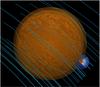 |
Fig. 1 Three-dimensional rendering of the MHD simulation RUN2_G, describing the expansion of SN 1006 through a magnetized medium and its interaction with an ambient cloud at t = 1000 yr (the model parameters are shown in Table 1). The image is rotated to match the actual conditions of SN 1006 and the orientation of the observations (north is up and east is to the left). The ejecta material and the shocked ambient medium are tracked with a “solid” and a semi-transparent surface, respectively. The cutaway drawing of the southwestern cloud reveals its interior: the color code traces the density, which increases radially from 0.07 cm-3 (dark blue) to 10 cm-3 (red). The magnetic field lines are superimposed. The (projected) gradient of the magnetic field points toward southeast. |
We considered the parameters of the cloud inferred from the observations in Paper I as fiducial values and ran different simulations around these observational estimates to constrain the physical properties of the cloud. In particular, the parameters explored include: i) the position and the radius of the cloud; ii) the position of the magnetic dipole (influencing the distance of the cloud to the polar caps of the remnant); iii) the cloud density; and iv) the radial density profile of the cloud, namely a uniform density profile (RUN1, 2_UN) and a centrally peaked Gaussian profile (RUN0-3_G). Table 1 summarizes our exploration of the parameter space. The cloud density, which is poorly constrained by the data analysis, varies by more than two orders of magnitude in runs RUN0-3_G. In these runs, we explored different distances of the cloud from the explosion site, therefore the SNR shock reaches different parts of the cloud at t = 1000 yr. This allowed us to study the effects of the propagation of the transmitted shock in the tenuous exterior part of the cloud (e.g., RUN1_G) or in its denser core (e.g., RUN0_G). The output of all our simulations were then rotated to match the actual conditions of SN 1006 and the orientation of the observations (where north is up and east is to the left). In particular, all the maps presented here are rotated by an angle αX = 15°, αZ = 8°, αY = 37°, about the x, z, and y axis, respectively (the rotations being performed in this order). With these rotations the magnetic field gradient points in the direction of the galactic plane, as suggested by Bocchino et al. (2011). As an example, Fig. 1 shows a rendering of the final stage of model RUN2_G. We also performed a convergence test, by increasing the resolution of model RUN2_G by a factor of 2, and found that the results do not differ significantly from those reported in Sect. 4.
Finally, we point out that Orlando et al. (2012) have shown that inhomogeneities in the ejecta density profile (“clumps”) can perturb the contact discontinuity and affect the distance between ejecta and shocked ISM, thus triggering the formation of shrapnel protruding even beyond the shock front (see also Miceli et al. 2013b). These ejecta clumps, well visible at different positions of the shell of SN 1006 (e.g., Rakowski et al. 2011; Winkler et al. 2014) are not present in the shock-interaction region we are modeling here (see the “pure thermal” image of the remnant in Miceli et al. 2009). Also, we are interested at modeling the interaction between the outer shock front and the ambient medium and not the details of the ejecta evolution. Therefore, we did not include ejecta clumps in our model.
3. Synthesis of observables
To get a quantitative comparison between our MHD models and actual observations of SN 1006, we followed a forward modeling approach, by synthesizing the emission from the simulations and comparing the synthesized observables and the corresponding data. The X-ray emission of the shock-cloud interaction region in the southwestern limb of SN 1006 is dominated by synchrotron radiation, the contribution of thermal emission being negligible (see Paper I). We then focused on the nonthermal emission and used REMLIGHT, a code developed to synthesize the synchrotron radio, X-ray, and IC γ-ray emission from MHD simulations, introduced and described in detail in Orlando et al. (2011). In particular, we derived the nonthermal emission in the loss-limited case (see Sect. 3.1 in Orlando et al. 2011), which is appropriate for the nonthermal limbs of SN 1006 (Miceli et al. 2013a, 2014b). The outputs of REMLIGHT are 3D data cubes of i) synchrotron monochromatic X-ray emission at selected energies; ii) cutoff energy of the electron spectrum; iii) IC monochromatic emission at selected energies.
3.1. Synthesis of X-ray emission
To produce synthetic X-ray images, we calculated the synchrotron 3D data cubes at 3 keV and summed the contribution of each cell to the emission along the line of sight. We also computed the cutoff energy hνcut of the X-ray synchrotron radiation, derived from the electron cutoff energy. In the loss limited scenario, it has the form (Zirakashvili & Aharonian 2007):  (1)where η is the gyrofactor (i.e., the ratio of the electron mean free path to the gyroradius), κ is the magnetic field compression ratio, v3000 is the shock speed in units of 3000 km s-1, and γs is the power-law index of particles accelerated at the absence of energy losses.
We included in our model two passive tracers (defined in the whole domain) storing the time of the shock impact and the shock velocity at the shock impact for each cell, respectively. As the fluid is advected away from the shock front, this information is used to update the electron energy spectrum. The value of hνcut varies with the azimuthal angle as explained before and with the distance to the shock, as the shape of the electron energy spectrum is modified by the radiative losses. We imposed the maximum value of hνcut to be  eV in the polar caps, in agreement with what is observed in the southwestern limb of SN 1006 (see Paper I). Then we calculated the “effective” synchrotron cutoff energy in specific regions of the synthetic X-ray image, by performing a weighted average of the cutoff energy along the line of sight for all the cells whose projected position lies within the region, the weight being the local X-ray luminosity (which is a good proxy of the actual X-ray luminosity in the southwestern limb of SN 1006, as shown in Sect. 4).
We point out that the parametric function adopted in our model to describe the shock obliquity dependence of the particle acceleration (described in Sect. 2) is purely heuristic and that we are not including the effects of magnetic field amplification (MFA). The physics of MFA at the shock precursor is still debated and extremely complicated, involving resonant and non-resonant cosmic-ray driven instabilities operating at different time scales and length scales (see the reviews by Bykov et al. 2012; and Schure et al. 2012). Different approaches have been adopted to treat this process and to couple it with the MHD evolution of a SNR (e.g., Amato & Blasi 2006; Caprioli 2012; Lee et al. 2012; Kang et al. 2013). Ferrand et al. (2014) considered two limit cases, namely, i) total damping of the amplified field in the plasma; ii) advection to the sub-shock region of the amplified field. They found that in the second case the post-shock magnetic field is one order of magnitude higher and this significantly influences the resulting synchrotron emission. In SN 1006 the situation is even more complicated, considering the (unknown) dependence of the efficiency of the particle acceleration (and then of the MFA) on the obliquity angle. To obtain the correct value of the post-shock magnetic field, we then tuned our ambient magnetic field so as to obtain B ~ 100μG at the polar caps, in agreement with the observations (Morlino et al. 2010; Ressler et al. 2014). However, even though we get the right magnetic field at the polar caps, its azimuthal profile may not reflect the actual conditions in the remnant and, as a consequence, the large-scale morphology of our synthetic X-ray synchrotron maps may not be an accurate proxy of the actual emission. However, the comparison between models and X-ray observations carried out here is not sensitive to this issue considering that i) the azimuthal extension of the interacting region is relatively small and concentrated in the polar cap region and that ii) the azimuthal modulation of the synchrotron cutoff frequency in the interaction region that we chose as a benchmark for a quantitative comparison between models and X-ray observations does not depend on B in the loss-limited scenario.
3.2. Synthesis of γ-ray emission
To derive the γ-ray synthetic spectral energy distribution, we adopted REMLIGHT to produce IC 3D data cubes at selected energies (in the 10-4−300 TeV range) and summed up the contribution of all the cells in the southwestern limb. We only considered IC scattering of the cosmic microwave background (CMB). Indeed, the expanding ejecta of young SNRs are expected to be important factories of cold dust, whose thermal infrared emission may also contribute to the total IC emission. However, a dedicated study performed with the Spitzer telescope at 24 μm and 70 μm showed no emission from the southwestern limb and, in general, no evidence for dust grain formation in the SN ejecta of SN 1006 (Winkler et al. 2013). On the other hand, Planck observations showed the presence of very cold gas (at a temperature Td ~ 15 K) in the direction of SN 1006 (Planck Collaboration XI 2014), but the association with the remnant cannot be proved. Therefore, we neglected any contributions from IR dust photons to the IC emission.
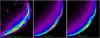 |
Fig. 2 Left panel: XMM-Newton EPIC count-rate image (MOS and pn mosaic) of the southwestern limb of SN 1006 in the 2−4.5 keV band. The regions selected for the spectral analysis of the rim performed in Paper I are superimposed. Central panel: synthetic synchrotron emission at 3 keV at t = 1000 yr derived from model RUN2_G (see Table 1). The regions selected to derive the azimuthal variation of the synchrotron cutoff energy at the shock front are superimposed. Right panel: same as central panel for model RUN2_UN. |
The recent results obtained by Acero et al. (2015) clearly indicate that the bulk of the SN 1006 γ-ray emission has a leptonic origin and rule out, at a confidence level >5σ, a standard hadronic emission scenario. Therefore, we rescaled the synthetic IC SED obtained with REMLIGHT (which is in arbitrary units) to fit the TeV HESS observations of the southwestern limb of SN 1006 (Acero et al. 2010).
We note that, because of the interaction with a dense cloud, the hadronic emission may have a non-negligible contribution in the Fermi − LAT band. To synthesize the hadronic γ-ray emission, we considered the particle density in each cell of the shocked ambient medium (distinguishing between ISM and cloud material). We assumed two populations of high-energy hadrons, both having a power law proton energy distribution (with index Γ = 2.0) and let the cutoff energy  of the protons accelerated at the shock transmitted inside the cloud (i.e., those colliding with the cloud material) be different from that of protons accelerated at the remnant forward shock and interacting with the tenuous ambient material (
 ). We explored different values of
  for the two populations, and of the total hadron energy in the southwestern limb,
  . We then computed in each cell the resulting hadronic emission at selected energies in the 10-4−300 TeV range and summed up all the contributions in the southwestern limb. The cross section for the proton-proton inelastic collision, the π0 production, and the γ-ray emission originating from the π0 decays were all obtained according to Kelner et al. (2006).
4. Results
4.1. X-ray emission
As a first step, we compared the synthetic X-ray images of SN 1006 with the actual observations in the 2−4.5 keV energy band. The X-ray data were collected in the framework of the XMM − LP and the data analysis is described in Paper I. Among the runs listed in Table 1, only models RUN2_G and RUN2_UN can reproduce the observed emission of the southwestern limb of SN 1006 in terms of azimuthal extension of the interacting region and depth of the indentation, as shown in Fig. 2.
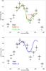 |
Fig. 3 Upper panel: azimuthal variations of the synchrotron cutoff energy. The black crosses show the best fit values obtained in Paper I by analyzing the X-ray spectra extracted from regions A − L of Fig. 2, left panel (error bars indicate the 90% confidence levels). The green/red curves show the values derived from our MHD models RUN2_G and RUN2_UN, respectively, by considering the 15 regions shown in the central and right panel of Fig. 2. The dashed crosses indicate the values in the bulge region. Lower panel: same as upper panel for model RUN1_G (blue curve). |
In RUN2_G the shocked cloud has an inward increasing density profile (in the range 0.07−10 cm-3) and is reached by the remnant shock front at t = 640 yr. For the first ~80 yr of interaction, the transmitted shock propagates relatively fast in the outermost parts of the cloud, being only a few percent slower than the remnant forward shock that engulfs the cloud. As the transmitted shock approaches the dense core of the cloud, its speed decreases significantly, reaching a minimum value of ~30% of the remnant shock speed at t = 1000 yr. At this stage, the density of the cloud material immediately behind the transmitted shock front is ~3 cm-3. In RUN2_UN the cloud has uniform density ncl = 0.5 cm-3 (~17 times higher than that of the surrounding medium). In this case, the cloud is slightly smaller than in RUN2_G and is reached by the remnant forward shock at t ~ 750 yr. At t = 1000 yr the minimum velocity of the transmitted shock is about 40% of the remnant shock speed, while the density of the shocked cloud material is ~1.5 cm-3.
In both models, the relatively low velocity of the transmitted shocks induces a drop in the synchrotron cutoff energy, which is lower by a factor f = 8−9 in the interaction region than in the other parts of the SN 1006 shock front. This is much higher than the observed drop of the cutoff frequency f ~ 1.7 derived in Paper I. However, the lateral (fast) shocks engulfing the cloud also contribute to the synchrotron emission in the (projected) interaction region and it is necessary to account for this effect to properly compare the models with the data. We then derived maps of X-ray emission projected in the plane of the sky and selected a set of 15 regions at the shock front (shown in the central and right panels of Fig. 2). We calculated the synchrotron cutoff energies in each region (as described in Sect. 3), and compared them to those obtained in Paper I from the analysis of the X-ray spectra extracted from regions A − L (shown in the left panel of 2). Upper panel of Fig. 3 shows the observed azimuthal profile of the cutoff energy and that derived with our models. Though RUN2_UN provides a slightly better description of the data points, both models can reproduce the observed dip in the cutoff energy and fit all the main features of the observed profile. This result shows that we cannot discriminate between the two models on the basis of the cutoff energy variations and that it is difficult to ascertain information on the cloud structure from this parameter, given the importance of the synchrotron emission from lateral shocks in the emerging X-ray radiation.
On the other hand, we verified that the azimuthal profile of the cutoff energy in all other runs do not fit the observations. As an example, lower panel of Fig. 3 shows the profile derived from RUN1_G, where the cloud is placed at a larger distance to the SNR center and produces a much smaller indentation than that obtained in RUN2_G. In this case, the dip in the cutoff energy profile is less pronounced and definitely not consistent with the data points.
We also calculated the cutoff energy in the relatively faint region “upstream” from the indentation, marked by the dashed contours in the central and right panels of Fig. 2, and compared it with that measured in the corresponding region of SN 1006 (named “bulge” in Paper I, white dashed region in the left panel of Fig. 2). The emission in this region originates in the non-interacting part of the shock front and, in model RUN2_G, is much softer than that observed (compare the red and black dashed line in Fig. 3). In RUN2_UN we achieve a better agreement between model and observations (green and black dashed line in Fig. 3, respectively). However, additional synchrotron emission from the bulge may arise from electrons produced by cosmic rays diffusing away from the southwestern limb in the nearby cloud and not included in our models. Also, deviations in the cloud morphology from the simple spherical/ellipsoidal shapes adopted in our simulations may affect the emission in this region. Therefore, we do not consider that these fits rule out model RUN2_G.
The different densities of the shocked cloud in RUN2_G and RUN2_UN induce differences in the velocity of the transmitted shock which, in turn, affects the proper motion of the indentation observed in the X-ray maps. To discriminate between the two models we then measured the proper motion of the indentation in RUN2_G and RUN2_UN, and in the southwestern limb of SN 1006. Winkler et al. (2014) performed a systematic study of the X-ray proper motion around the whole periphery of SN 1006 by comparing the observations of the Chandra − LP with previous Chandra images obtained from 2003 observations and found a local minimum at the position of the indentation (azimuthal angle θ ~ 245°). To resolve with higher resolution the azimuthal profile of the proper motion in the shock-cloud interaction region, we repeated their analysis by defining the 5 regions shown in the upper panel of Fig. 4. As for the models, we adopted the same procedure, by selecting narrow stripes (10 pixels wide) perpendicular to the limb in the synthetic X-ray images and deriving the average radial profiles therein. We selected a much wider region in the indentation (spanning 10 degrees), as done for the real data. The error bars in the proper motion estimated by our models are sensitivity errors associated with the spatial resolution of the computational grid. Because of the limited spatial resolution of our simulations, we adopted a baseline of 40 yr. Lower panel of Fig. 4 shows the comparison between the observed proper motion (black crosses) and that predicted by model RUN2_G (red) and RUN2_UN (green). We confirm that the proper motion measured in the indentation of SN 1006 with Chandra is significantly lower than that measured immediately outside the indentation and in the bulge. This result provides further observational evidence of the shock-cloud interaction occurring in the southwestern limb. RUN2_G predicts a decrease in the proper motion of the indentation which is much higher than that measured. On the other hand, the proper motion predicted by RUN2_UN is in very good agreement with the data, both for the indentation and for the bulge.
We conclude that RUN2_UN is the model that best describes the X-ray emission resulting from the interaction of the SN 1006 southwestern shock front and the ambient cloud. This model, in fact, can explain: i) the morphology of the synchrotron emitting southwestern limb; ii) the azimuthal variations of the cutoff energy of the X-ray synchrotron emission; iii) the azimuthal profile of the proper motion.
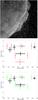 |
Fig. 4 Upper panel: Chandra ACIS close-up view of the SN 1006 southwestern limb in the 0.5−7 keV band. The regions selected for proper-motion measurements are shown in white. Central panel: azimuthal variation of the proper motion (normalized to its maximum value) in the southwestern limb of SN 1006 measured with Chandra (black crosses) and predicted by models RUN2_G (red crosses). Lower panel: same as central panel for RUN2_UN (green crosses). The dashed crosses refer to the bulge region. Error bars indicate the 1σ confidence level for the X-ray data (black solid lines) and the sensitivity errors for the models. |
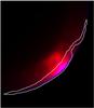 |
Fig. 5 Synthetic inverse Compton monochromatic emission of the southwestern limb of SN 1006 at 3 GeV (in red) and 3 TeV (in blue) derived from RUN2_UN. The contours of the X-ray emission are superimposed in white. |
4.2. γ-ray emission
Though expanding in a tenuous environment, almost six hundred pc above the Galactic plane, SN 1006 interacts with ambient interstellar clouds. A higher ambient density is observed in the northwestern rim, where the shock is slowed down by the interaction with dense material (the northwestern cloud), producing a relatively bright and sharp Hα filament and soft X-ray emission (e.g., Ghavamian et al. 2002; Winkler et al. 2003; Raymond et al. 2007; Acero et al. 2007; Li et al. 2015). Nikolić et al. (2013) have revealed suprathermal hadrons in the northwestern limb of SN 1006, but particle acceleration is not very efficient therein, as revealed by the very faint nonthermal emission. The southwestern limb, instead, shows both efficient particle acceleration and relatively high ambient density in the cloud, thus being a privileged site for the detection of γ-ray hadronic emission.
In Paper I we proposed a rough estimate of the expected emission on the basis of the radio and X-ray data analysis and we obtained a flux of ~5 × 10-13 erg cm-2 s-1 in the 3−30 GeV band, by assuming a cloud density of 10 cm-3. This flux was slightly below the Fermi − LAT upper limit available. However, the subsequent analysis of six years of Fermi − LAT data performed by Acero et al. (2015) has recently provided more stringent constraints which seem to rule out a possible hadronic origin for the bulk of the γ-ray emission of both the southwestern and northeastern limbs of SN 1006. In particular, the upper limits (at the 95% confidence level) for the flux of the southwestern limb are ~1.9 × 10⁻¹³ erg cm-2 s-1 at the median energy of the 3−30 GeV (i.e., at 9.48 GeV) band and ~3.5 × 10⁻¹³ erg cm-2 s-1 at 94.8 GeV.
Here, we can refine our predictions taking advantage of the results of the MHD simulations that allowed us to tightly constrain the cloud density and the mass of the shocked cloud material. The detailed description of the targets of the proton-proton collisions leaves only the spectrum of the accelerated particle as a free parameter to derive the possible hadron emission from SN 1006, thus allowing us to ascertain some properties of the cosmic rays accelerated at the SW limb of SN 1006. In particular, we explored what values of and are consistent with the observational constraints on the γ-ray emission.
To synthesize the γ-ray emission we then focused on our best-fit model RUN2_UN and considered three components, namely i) the IC emission; ii) the hadronic emission originating from the impact of high-energy protons with the cloud material; and iii) the hadronic emission originating from the impact of high-energy protons with the ambient tenuous medium (see Sect. 3.2 for details).
Fig. 5 shows the synthetic IC emission at 3 GeV (in red) and 3 TeV (in blue) obtained from RUN2_UN (a very similar map is obtained for RUN2_G). As expected, the TeV emission, which is associated with electrons at energies E> 10 TeV, is concentrated in the immediate post-shock region. The high-energy electrons lose rapidly their energy via radiative cooling as they are advected in the post-shock region and this makes the TeV emission radially thin (and pretty similar to the X-ray synchrotron emission). Electrons with energies of a few 1011 eV, which up-scatter the CMB photons up to GeV energies, are instead present at larger distances from the shock front, thus making the GeV emission much broader in the radial direction.
As for the hadron emission, we first explored the case proposed in Paper I, with  erg (i.e. a total hadronic energy
  erg in the whole remnant, corresponding to ~10% of the explosion energy),
  TeV, and
  TeV. We verified that, with this set of parameters, the resulting γ-ray emission is well above the latest Fermi − LAT upper limits, as shown in the upper panel of Fig. 6. We stress that the same happens also for RUN2_G, where, in general, we get higher hadronic emission, given the higher average density of the shocked cloud.
We then explored different proton spectra, by reducing the total hadronic energy. Central panel of Fig. 6 shows the synthetic γ-ray emission obtained for  erg (i.e., hadrons have drained ~5% of the explosion energy), TeV, and TeV. With this set of parameters, the synthetic spectrum fits the observed HESS spectrum at TeV energy (where the IC contribution dominates) and is consistent with the newest Fermi − LAT upper limits, being at the edge of detectability in the 3−30 GeV band. This emission, if present, will be detectable within a few more years. We note that a claim for a likely Fermi detection of SN 1006 has been recently proposed by Xing et al. (2016). Lower panel of Fig. 6 shows the γ-ray emission for
  erg: in this case, the γ-ray flux is well below the Fermi − LAT upper limits.
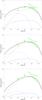 |
Fig. 6 Upper panel: synthetic γ-ray emission of the southwestern limb of SN 1006 obtained from RUN2_UN by assuming a total hadronic energy |
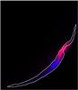 |
Fig. 7 Synthetic γ-ray (hadronic+leptonic) monochromatic emission of the southwestern limb of SN 1006 at 3 GeV (in red) and 3 TeV (in blue) derived from RUN2_UN with |
5. Summary and conclusions
We performed a set of 3D MHD simulations describing the evolution of SN 1006 and its interaction with an ambient cloud. Taking into account the estimates derived with the radio and X-ray data analysis performed in Paper I, we explored different simulation setups by modifying the properties of the ambient cloud and magnetic field. We adopted a forward modeling approach by synthesizing observables from the simulations and comparing them against actual data.
We first focused on the X-ray morphology and identified two possible configurations, namely RUN2_G and RUN2_UN, whose synchrotron X-ray maps exhibit a net indentation in the X-ray southwestern limb, corresponding to the shock-cloud interaction region, which is in very good agreement with the X-ray observations. We also verified that both these runs can explain the observed azimuthal profile of the synchrotron cutoff energy. In RUN_2G, the cloud has a radius Rcl = 8.1 × 1018 cm) and an inward increasing density profile (spanning from 0.07 cm-3 up to 10 cm-3). The downstream density is ~3 cm-3 at the stage of evolution corresponding to the current conditions of SN 1006. In RUN2_UN the cloud is slightly smaller (Rcl = 6.18 × 1018 cm), but has a uniform density ncl = 0.5 cm-3. The 3D modeling and the synthesis of the observables allowed us to explain the relatively low dip observed in the cutoff energy azimuthal profile, which appeared to be much lower than that expected by considering the cloud/ISM density contrast. In particular, we showed that the drop in the cutoff energy cannot be used as a reliable density contrast indicator because it does not trace the interacting region alone; it is also affected by the synchrotron emission originating from lateral shocks and integrated along the line of sight. To discriminate between the two models we then measured the proper motion of the X-ray emitting southwestern limb and found that only RUN2_UN provides results in agreement with that measured with the most recent Chandra observations. Therefore, the quantitative comparison between our models and X-ray data allowed us to explain all the puzzling features observed in the southwestern limb of SN 1006 (morphology, spectral inhomogeneities of the synchrotron emission, and azimuthal variations of the proper motion).
We tightly constrained the cloud density and the mass of the shocked cloud. In particular, we found that the pre-shock density of the cloud is 0.5 cm-3. In Paper I we estimated a higher cloud density from the HI data (~10 cm-3). However, we point out that the density estimate derived in Paper I strongly relies on (arbitrary) assumptions about the cloud geometry and its extension along the line of sight. Furthermore, the bulk of the HI cloud is still unshocked, so its density may be higher than that of the interacting part. We also note that our density estimate is similar to that derived for the northwestern cloud (Raymond et al. 2007; Acero et al. 2007), which is probably physically connected with the southwestern cloud, as suggested in Paper I. Future observations of the 12CO emission (in the 2−1 line transition) are planned in the direction of the interacting HI gas to resolve the cloud internal structure and identify the scale of gas clumpiness, which will then be compared with the predicted physical conditions.
The determination of the cloud properties obtained with our model is crucial because the hadronic γ-ray emission depends on the spectrum of the accelerated cosmic rays and on the ambient density. Therefore the knowledge of the physical parameters of the shocked cloud allowed us to ascertain information on the hadronic acceleration in the southwestern limb. In particular, we found that if we assume that the total cosmic ray energy is 10% of the explosion energy (i.e., the hadronic energy in the southwestern limb is 5 × 1049 erg), the γ-ray emission from the shocked cloud is expected to be much higher than the current Fermi − LAT upper limit (as shown in Fig. 6). We therefore have to exclude such an efficient energy drain, unless we impose that the cutoff energy of the proton spectrum in the shock-cloud interaction region is much lower than our assumed value TeV. In this case, the “hadronic bump” would be centered at much lower energies, well below the Fermi − LAT sensitivity band.
However, if the proton cutoff energy is on the order of a few TeV we derive that the upper limit for the hadronic energy in the southwestern limb is 2.5 × 1049 erg (indicating a total hadronic energy on the order of ~5% of the explosion energy). For such an energy value we expect to observe a significant hadronic emission originating in the shock-cloud interaction region and detectable with Fermi − LAT within a few years. This emission will be concentrated in the shock-cloud interaction, as shown in Fig. 7. A non-detection would imply a much lower energy for the cosmic rays accelerated at the shock front.
Because  .
.
Acknowledgments
We thank the anonymous referee for their comments and suggestions. The software used in this work was in part developed by the DOE-supported ASC/Alliance Center for Astrophysical Thermonuclear Flashes at the University of Chicago. We acknowledge the HPC facility at CINECA, Italy, and the HPC facility SCAN of the INAF – Osservatorio Astronomico di Palermo for the availability of high-performance computing resources and support. This paper was partially funded by the PRIN INAF 2014 grant “Filling the gap between supernova explosions and their remnants through magnetohydrodynamic modeling and high-performance computing”. M.M. thanks E. Amato for interesting discussions and suggestions. V.P. acknowledges the support of the Spanish Ministerio de Economía y Competitividad through grant AYA2011-29754-C03. P.F.W. acknowledges the support of the National Aeronautics and Space Administration through Chandra Grant Number GO2-13066. The work of G.D. is funded by PICT-ANPCyT 0571/11 and PIP-CONICET 0736/11 of Argentina.
References
- Acero, F., Ballet, J., & Decourchelle, A. 2007, A&A, 475, 883 [NASA ADS] [CrossRef] [EDP Sciences] [Google Scholar]
- Acero, F., Aharonian, F., Akhperjanian, A. G., et al. 2010, A&A, 516, A62 [NASA ADS] [CrossRef] [EDP Sciences] [Google Scholar]
- Acero, F., Lemoine-Goumard, M., Renaud, M., et al. 2015, A&A, 580, A74 [NASA ADS] [CrossRef] [EDP Sciences] [Google Scholar]
- Amato, E., & Blasi, P. 2006, MNRAS, 371, 1251 [NASA ADS] [CrossRef] [Google Scholar]
- Berezhko, E. G., Ksenofontov, L. T., & Völk, H. J. 2012, ApJ, 759, 12 [NASA ADS] [CrossRef] [Google Scholar]
- Blasi, P. 2002, Astropart. Phys., 16, 429 [Google Scholar]
- Blasi, P. 2004, Astropart. Phys., 21, 45 [Google Scholar]
- Bocchino, F., Orlando, S., Miceli, M., & Petruk, O. 2011, A&A, 531, A129 [NASA ADS] [CrossRef] [EDP Sciences] [Google Scholar]
- Broersen, S., Vink, J., Miceli, M., et al. 2013, A&A, 552, A9 [NASA ADS] [CrossRef] [EDP Sciences] [Google Scholar]
- Bykov, A. M., Ellison, D. C., & Renaud, M. 2012, Space Sci. Rev., 166, 71 [NASA ADS] [CrossRef] [Google Scholar]
- Caprioli, D. 2012, J. Cosmol. Astropart. Phys., 7, 038 [NASA ADS] [CrossRef] [Google Scholar]
- Chevalier, R. A. 1982, ApJ, 258, 790 [NASA ADS] [CrossRef] [Google Scholar]
- Ferrand, G., Decourchelle, A., Ballet, J., Teyssier, R., & Fraschetti, F. 2010, A&A, 509, L10 [NASA ADS] [CrossRef] [EDP Sciences] [Google Scholar]
- Ferrand, G., Decourchelle, A., & Safi-Harb, S. 2014, ApJ, 789, 49 [NASA ADS] [CrossRef] [Google Scholar]
- Fryxell, B., Olson, K., Ricker, P., et al. 2000, ApJS, 131, 273 [NASA ADS] [CrossRef] [Google Scholar]
- Ghavamian, P., Winkler, P. F., Raymond, J. C., & Long, K. S. 2002, ApJ, 572, 888 [NASA ADS] [CrossRef] [Google Scholar]
- Green, D. A. 2009, Bull. Astron. Soc. India, 37, 45 [Google Scholar]
- Kang, H., Jones, T. W., & Edmon, P. P. 2013, ApJ, 777, 25 [NASA ADS] [CrossRef] [Google Scholar]
- Katsuda, S., Petre, R., Long, K. S., et al. 2009, ApJ, 692, L105 [NASA ADS] [CrossRef] [Google Scholar]
- Katsuda, S., Petre, R., Mori, K., et al. 2010, ApJ, 723, 383 [NASA ADS] [CrossRef] [Google Scholar]
- Katsuda, S., Long, K. S., Petre, R., et al. 2013, ApJ, 763, 85 [NASA ADS] [CrossRef] [Google Scholar]
- Kelner, S. R., Aharonian, F. A., & Bugayov, V. V. 2006, Phys. Rev. D, 74, 034018 [NASA ADS] [CrossRef] [Google Scholar]
- Lee, S.-H., Ellison, D. C., & Nagataki, S. 2012, ApJ, 750, 156 [NASA ADS] [CrossRef] [Google Scholar]
- Li, J.-T., Decourchelle, A., Miceli, M., Vink, J., & Bocchino, F. 2015, MNRAS, 453, 3953 [NASA ADS] [CrossRef] [Google Scholar]
- Miceli, M., Bocchino, F., Iakubovskyi, D., et al. 2009, A&A, 501, 239 [NASA ADS] [CrossRef] [EDP Sciences] [Google Scholar]
- Miceli, M., Bocchino, F., Decourchelle, A., et al. 2012, A&A, 546, A66 [NASA ADS] [CrossRef] [EDP Sciences] [Google Scholar]
- Miceli, M., Bocchino, F., Decourchelle, A., et al. 2013a, A&A, 556, A80 [NASA ADS] [CrossRef] [EDP Sciences] [Google Scholar]
- Miceli, M., Orlando, S., Reale, F., Bocchino, F., & Peres, G. 2013b, MNRAS, 430, 2864 [NASA ADS] [CrossRef] [Google Scholar]
- Miceli, M., Acero, F., Dubner, G., et al. 2014a, ApJ, 782, L33 [NASA ADS] [CrossRef] [Google Scholar]
- Miceli, M., Bocchino, F., Decourchelle, A., et al. 2014b, Astron. Nachr., 335, 252 [NASA ADS] [CrossRef] [Google Scholar]
- Morlino, G., Amato, E., Blasi, P., & Caprioli, D. 2010, MNRAS, 405, L21 [NASA ADS] [Google Scholar]
- Nikolić, S., van de Ven, G., Heng, K., et al. 2013, Science, 340, 45 [NASA ADS] [CrossRef] [Google Scholar]
- Orlando, S., Bocchino, F., Reale, F., Peres, G., & Petruk, O. 2007, A&A, 470, 927 [NASA ADS] [CrossRef] [EDP Sciences] [Google Scholar]
- Orlando, S., Petruk, O., Bocchino, F., & Miceli, M. 2011, A&A, 526, A129 [NASA ADS] [CrossRef] [EDP Sciences] [Google Scholar]
- Orlando, S., Bocchino, F., Miceli, M., Petruk, O., & Pumo, M. L. 2012, ApJ, 749, 156 [NASA ADS] [CrossRef] [Google Scholar]
- Petruk, O., Bocchino, F., Miceli, M., et al. 2009, MNRAS, 399, 157 [NASA ADS] [CrossRef] [Google Scholar]
- Planck Collaboration XI. 2014, A&A, 571, A11 [NASA ADS] [CrossRef] [EDP Sciences] [Google Scholar]
- Rakowski, C. E., Laming, J. M., Hwang, U., et al. 2011, ApJ, 735, L21 [NASA ADS] [CrossRef] [Google Scholar]
- Raymond, J. C., Korreck, K. E., Sedlacek, Q. C., et al. 2007, ApJ, 659, 1257 [NASA ADS] [CrossRef] [Google Scholar]
- Ressler, S. M., Katsuda, S., Reynolds, S. P., et al. 2014, ApJ, 790, 85 [NASA ADS] [CrossRef] [Google Scholar]
- Reynolds, S. P. 2008, ARA&A, 46, 89 [Google Scholar]
- Reynoso, E. M., Hughes, J. P., & Moffett, D. A. 2013, AJ, 145, 104 [NASA ADS] [CrossRef] [Google Scholar]
- Rothenflug, R., Ballet, J., Dubner, G., et al. 2004, A&A, 425, 121 [NASA ADS] [CrossRef] [EDP Sciences] [Google Scholar]
- Schure, K. M., Bell, A. R., O’C Drury, L., & Bykov, A. M. 2012, Space Sci. Rev., 173, 491 [NASA ADS] [CrossRef] [EDP Sciences] [Google Scholar]
- Uchida, H., Yamaguchi, H., & Koyama, K. 2013, ApJ, 771, 56 [NASA ADS] [CrossRef] [Google Scholar]
- Vink, J. 2012, A&ARv, 20, 49 [Google Scholar]
- Winkler, P. F., Gupta, G., & Long, K. S. 2003, ApJ, 585, 324 [NASA ADS] [CrossRef] [Google Scholar]
- Winkler, P. F., Williams, B. J., Blair, W. P., et al. 2013, ApJ, 764, 156 [NASA ADS] [CrossRef] [Google Scholar]
- Winkler, P. F., Williams, B. J., Reynolds, S. P., et al. 2014, ApJ, 781, 65 [NASA ADS] [CrossRef] [Google Scholar]
- Xing, Y., Wang, Z., Zhang, X., & Chen, Y. 2016, ApJ, 823, 44 [NASA ADS] [CrossRef] [Google Scholar]
- Zirakashvili, V. N., & Aharonian, F. 2007, A&A, 465, 695 [NASA ADS] [CrossRef] [EDP Sciences] [Google Scholar]
All Tables
All Figures
|
Fig. 1 Three-dimensional rendering of the MHD simulation RUN2_G, describing the expansion of SN 1006 through a magnetized medium and its interaction with an ambient cloud at t = 1000 yr (the model parameters are shown in Table 1). The image is rotated to match the actual conditions of SN 1006 and the orientation of the observations (north is up and east is to the left). The ejecta material and the shocked ambient medium are tracked with a “solid” and a semi-transparent surface, respectively. The cutaway drawing of the southwestern cloud reveals its interior: the color code traces the density, which increases radially from 0.07 cm-3 (dark blue) to 10 cm-3 (red). The magnetic field lines are superimposed. The (projected) gradient of the magnetic field points toward southeast. |
| In the text | |
|
Fig. 2 Left panel: XMM-Newton EPIC count-rate image (MOS and pn mosaic) of the southwestern limb of SN 1006 in the 2−4.5 keV band. The regions selected for the spectral analysis of the rim performed in Paper I are superimposed. Central panel: synthetic synchrotron emission at 3 keV at t = 1000 yr derived from model RUN2_G (see Table 1). The regions selected to derive the azimuthal variation of the synchrotron cutoff energy at the shock front are superimposed. Right panel: same as central panel for model RUN2_UN. |
| In the text | |
|
Fig. 3 Upper panel: azimuthal variations of the synchrotron cutoff energy. The black crosses show the best fit values obtained in Paper I by analyzing the X-ray spectra extracted from regions A − L of Fig. 2, left panel (error bars indicate the 90% confidence levels). The green/red curves show the values derived from our MHD models RUN2_G and RUN2_UN, respectively, by considering the 15 regions shown in the central and right panel of Fig. 2. The dashed crosses indicate the values in the bulge region. Lower panel: same as upper panel for model RUN1_G (blue curve). |
| In the text | |
|
Fig. 4 Upper panel: Chandra ACIS close-up view of the SN 1006 southwestern limb in the 0.5−7 keV band. The regions selected for proper-motion measurements are shown in white. Central panel: azimuthal variation of the proper motion (normalized to its maximum value) in the southwestern limb of SN 1006 measured with Chandra (black crosses) and predicted by models RUN2_G (red crosses). Lower panel: same as central panel for RUN2_UN (green crosses). The dashed crosses refer to the bulge region. Error bars indicate the 1σ confidence level for the X-ray data (black solid lines) and the sensitivity errors for the models. |
| In the text | |
|
Fig. 5 Synthetic inverse Compton monochromatic emission of the southwestern limb of SN 1006 at 3 GeV (in red) and 3 TeV (in blue) derived from RUN2_UN. The contours of the X-ray emission are superimposed in white. |
| In the text | |
|
Fig. 6 Upper panel: synthetic γ-ray emission of the southwestern limb of SN 1006 obtained from RUN2_UN by assuming a total hadronic energy |
| In the text | |
|
Fig. 7 Synthetic γ-ray (hadronic+leptonic) monochromatic emission of the southwestern limb of SN 1006 at 3 GeV (in red) and 3 TeV (in blue) derived from RUN2_UN with |
| In the text | |
Current usage metrics show cumulative count of Article Views (full-text article views including HTML views, PDF and ePub downloads, according to the available data) and Abstracts Views on Vision4Press platform.
Data correspond to usage on the plateform after 2015. The current usage metrics is available 48-96 hours after online publication and is updated daily on week days.
Initial download of the metrics may take a while.