| Issue |
A&A
Volume 693, January 2025
|
|
|---|---|---|
| Article Number | A193 | |
| Number of page(s) | 8 | |
| Section | Interstellar and circumstellar matter | |
| DOI | https://doi.org/10.1051/0004-6361/202451944 | |
| Published online | 17 January 2025 | |
Hadronic particle acceleration in the supernova remnant SN 1006 as traced by Fermi-LAT observations
1
Univ. Bordeaux, CNRS,
LP2i Bordeaux, UMR 5797,
33170
Gradignan,
France
2
AIM, CEA, CNRS, Université Paris-Saclay, Université de Paris,
91191
Gif sur Yvette,
France
3
FSLAC IRL 2009, CNRS/IAC,
La Laguna,
Tenerife,
Spain
4
Dipartimento di Fisica e Chimica E. Segrè, Università degli Studi di Palermo,
Piazza del Parlamento 1,
90134
Palermo,
Italy
5
INAF – Osservatorio Astronomico di Palermo,
Piazza del Parlamento 1,
90134
Palermo,
Italy
★ Corresponding author; This email address is being protected from spambots. You need JavaScript enabled to view it.
Received:
21
August
2024
Accepted:
10
December
2024
Abstract
The supernova remnant SN 1006 is a source of high-energy particles detected in the radio, X-rays, and tera-electronvolt gamma rays. It was also announced as a source of gamma rays by Fermi-LAT, but only the north-east (NE) limb was detected at a significance level of more than 5σ. Using 15 years of Fermi-LAT observations and a thorough morphological analysis above 1 GeV, we report the detection of the NE rim at the 6σ level and the south–west (SW) rim at the 5.5σ level using radio templates from the GLEAM survey. The spectral analysis performed between 100 MeV and 1 TeV allows for the detection of a hard spectral index for the NE limb of 1.7 ± 0.1 ± 0.1, while the emission detected in the SW is reproduced well with a steeper spectral index of 2.2 ± 0.1 ± 0.1. A marginal detection (~3σ) of emission coincident with the bright north-west Hα filament is also described with a similar spectral index of ~2.1. We have successfully characterised the non-thermal multi-wavelength emission of the NE and SW limbs with a model in which inverse-Compton emission dominates in the NE, while proton-proton interactions becomes significant in the SW due to the enhanced density of the medium.
Key words: cosmic rays / ISM: supernova remnants / supernovae: individual: SN 1006
© The Authors 2025
 Open Access article, published by EDP Sciences, under the terms of the Creative Commons Attribution License (https://creativecommons.org/licenses/by/4.0), which permits unrestricted use, distribution, and reproduction in any medium, provided the original work is properly cited.
This article is published in open access under the Subscribe to Open model. This email address is being protected from spambots. You need JavaScript enabled to view it. to support open access publication.
1 Introduction
Located at 2.2 kpc from Earth (Winkler et al. 2003), the type Ia supernova remnant (SNR) SN 1006 is one of the few historical remnants observed from Earth. It is an ideal target with which to study the Fermi acceleration process in astrophysical shocks. Indeed, it is the first SNR in which a non-thermal component of hard X-rays was detected in the rims of the remnant by ASCA (Koyama et al. 1995), providing clear evidence for diffusive shock acceleration of electrons to high energies in the north– east (NE) and south–west (SW) limbs. Indications of efficient hadronic acceleration in the non-thermal limbs have also been provided recently (Giuffrida et al. 2022). High-resolution images by Chandra then revealed small-scale structure in the nonthermal X-ray filaments of the NE rim of SN 1006 (Long et al. 2003), supporting the idea of high magnetic fields in the bright limbs of the remnant. Deep observations at very high energy (VHE: above 100 GeV) were carried out with the H.E.S.S. telescopes from 2003 to 2008, allowing for the detection of a bipolar morphology, strongly correlated with the non-thermal X-rays (Acero et al. 2010). The two H.E.S.S. sources J1504–418 and J1502–421 correspond to the NE and SW shell regions and share similar flux values. Using 3.5 and 6 years of Fermi-Large Area Telescope (LAT) data, only upper limits have been obtained by Araya & Frutos (2012) and Acero et al. (2015), respectively. The detection at a 4σ level of a γ-ray source coincident with SN 1006 was claimed by Xing et al. (2016) using 7 years of LAT data. This was then confirmed by Condon et al. (2017) using 8 years of data, which enabled the detection of the SNR at 6σ as well as indication of an asymmetry of the high-energy γ-ray emission between the NE and SW regions. Xing et al. (2019) finally announced the detection of the SW limb at a 4σ significance level using 10 years of data. By performing broadband SED modelling of the two limbs, the authors concluded that, similarly to the case of the NE limb, the gamma-ray emission from the SW limb is likely dominated by the leptonic process in which high-energy electrons accelerated from the shell of the SNR inverse-Compton scatter background photons.
In this work, we aim to characterise the γ-ray emission detected at giga-electronvolt energies with Fermi-LAT using 15 years of observations (Section 2), and to undertake a full morphological analysis of the SNR (Section 3) and a spectral analysis of the different spatial components detected (Section 4). The results are then discussed using one-zone modelling of the multi-wavelength data (Section 5).
2 Fermi-LAT observations
The Fermi-LAT is a γ-ray telescope that detects photons by converting them into electron-positron pairs in the range from 20 MeV to higher than 500 GeV (Atwood et al. 2009). The following analysis was performed using 15 years of Fermi-LAT data (August 4 2008–August 3 2023) centred on SN 1006. Time intervals during which the satellite passed through the South Atlantic Anomaly were excluded. Our data were also filtered, removing time intervals around solar flares and bright gamma-ray bursts (GRBs), following the procedure used in all Fermi-LAT catalogs. The current version of the LAT data is P8R3 (Bruel et al. 2018). We used SOURCE class event selection, with the instrument response functions P8R3_SOURCE_V3. The Galactic diffuse emission was modelled by the standard file gll_iem_v07.fits and the residual background and extragalactic radiation are described by a single isotropic component with the spectral shape in the tabulated model iso_P8R3_SOURCE_V3_PSFn_v1.txt. The models are available from the Fermi Science Support Center (FSSC)1. The data reduction and exposure calculations were performed using the LAT fermitools version 2.2.0 and fermipy (Wood et al. 2017) version 1.2.0. We performed a binned likelihood analysis with 10 energy bins per decade over a region of 15° × 15°. We included all sources from the LAT 14-year source Catalog (4FGL-DR4)2 in a region of 25° × 25°. We accounted for the effect of energy dispersion (when the reconstructed energy differs from the true energy) by setting the parameter edisp_bins = –2. As such, the energy dispersion correction operates on the spectra with two extra bins below and above the threshold of the analysis3.
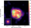 |
Fig. 1 Fermi-LAT TS map above 1 GeV for the 1.5° × 1.5° region around the SNR SN 1006. The black cross indicates the only 4FGL- DR4 source in the region (4FGL J1503.6–4146), while the magenta cross indicates the point source coincident with the SW rim added in our best model. The cyan contours represent the H.E.S.S. significance contours at 3, 5, and 7σ (Acero et al. 2010). White contours show the Hα template generated from the 4m Blanco telescope observations at CTIO (Winkler et al. 2014). Yellow contours present the radio spatial template derived using observations from the Murchison Widefield Array (Hurley-Walker et al. 2017). The inset on the bottom left corner provides the counts map from a simulated point source in the same coordinate system (more details in Appendix A). |
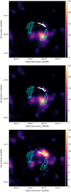 |
Fig. 2 Fermi-LAT TS map above 1 GeV after removing one of the three components from the best spatial model (Model 6, see Table 1): the H.E.S.S. NE limb (top panel), the Point source in the SW (middle panel), and the Hα component (bottom panel) with a reduced colour scale. For all TS maps, we present the 1.5° × 1.5° ROI around SN 1006. The cyan contours represent the H.E.S.S. significance contours at 3, 5, and 7σ (Acero et al. 2010). White contours show the Hα template used in our analysis. |
Results of the fit of the LAT data between 1 GeV and 1 TeV using different spatial models.
3 Morphological analysis of the LAT data
The morphological analysis was done between 1 GeV and 1 TeV to take advantage of the improved point spread function (PSF)4 (with a 68% containment radius smaller than 0.2° above 10 GeV). More details on the LAT PSF associated with our configuration are provided in Appendix A, in which we simulate a point source with a spectral index of 2.0. This simulation was added as an inset of Figure 1 to better visualise structures larger than our PSF.
We performed a binned analysis using all event types5 (PSF0, PSF1, PSF2, and PSF3) with spatial bins of 0.03°. As a first step, the spectral parameters of the sources located up to 3° from the centre of the region of interest (ROI) were fitted simultaneously with the Galactic and isotropic diffuse emissions. During this procedure, the 4FGL-DR4 power-law spectral model of the point source 4FGL J1503.6–4146 was used to reproduce the γ- ray emission of the SNR SN 1006. This source is coincident with the NE limb of the SNR and the only one included in the 4FGL-DR4 catalog located within a 1° radius from the centre of the SNR. To search for additional sources in the ROI, we computed a test statistic (TS) map that tests at each pixel the significance of a source with a generic E–2 spectrum against the null hypothesis: TS = 2(lnℒ1 – In ℒ0), where ℒ0 and ℒ1 are the likelihoods of the background (null hypothesis) and the hypothesis being tested (source plus background). We iteratively added two point sources in the model where the TS exceeded 25. We localised the two additional sources (RAJ2000 , DecJ2000 = 223.36° ± 0.03°, –45.62° ± 0.02°; 225.58° ± 0.03°, –42.04° ± 0.03°) and we fitted their power-law spectral parameters. The second point source is coincident with the SW limb, as can be seen in Figures 1 and 2 (middle), proving that the southern part of the SNR is now detected by the LAT with a TS value exceeding 25, assuming a point source hypothesis. We also calculated the improvement assuming extended Gaussians for these two additional sources and obtained TSext = 0 for the first source and 12 (below the threshold of 16 to claim for an extension) for the source coincident with the SW limb, which is called PS in the following. We then performed the morphological analysis of the SNR SN 1006. At each step, we replaced the point sources associated with the NE and SW limb of the emission with different geometrical and multi-wavelength templates, fitting both the morphological and spectral parameters of the new components. The results of all morphological tests performed are reported in Table 1. Since we cannot use the likelihood ratio test to compare models that are not nested, we used the Akaike information criterion (Akaike 1998, AIC). We calculated ∆AIC = AIC2pointsources – AICi = 2 × (∆ d.o.f. – ∆ln ℒ) to compare the different models. The different steps of the procedure are the following: fitting a disc, replacing the disc with the H.E.S.S. spatial template (Acero et al. 2010), or using a H.E.S.S. template for each limb separately. This last step provides an excellent fit to the data, though some residuals are still apparent on the NW of the SNR, coincident with the bright Hα filament, as can be seen in Figure 2 (right). The significance of this emission was tested by using an Hα spatial template generated from 4m Blanco telescope observations at CTIO (Winkler et al. 2014) in addition to the NE and SW H.E.S.S. templates, providing a better ∆AIC value (Model 5). Despite the larger number of degrees of freedom (d.o.f.), the best ∆AIC value is provided with a spatial model replacing the SW H.E.S.S. spatial template by the point source PS J1502.2–4203 (Model 6). This tends to demonstrate that the emission detected by the LAT does not correlate perfectly with the one observed at tera-electronvolt energies, despite a 3σ indication for an extension, and might have another origin. This will be discussed further in Section 5.
We also tested a radio spatial template (Model 7) using observations from the GLEAM survey performed with the Murchison Widefield Array (MWA) between 170 and 230 MHz (Hurley-Walker et al. 2017). This spatial template provides on its own an excellent fit to the data, as can be seen from the log-likelihood value in in Table 1. Then, dividing the radio spatial template to fit independently the NE and SW limb further improves the quality of the fit. In this case, the associated spectral indices differ by 2.7σ (the NE limb being harder than the SW one), confirming the previous indication of asymmetry derived by Condon et al. (2017). However, the best spatial model remains Model 6 even when fitting the NE and SW H.E.S.S. components in addition to the radio template.
Finally, focussing on the southern point source, we fixed its position at the coordinates of the nearby active galactic nucleus (AGN) candidate detected using NuSTAR observations (SW point source 2 located at RAJ2000 = 225.51°, DecJ2000 = –42.03°) by Li et al. (2018), which degrades the likelihood by 3.7 with respect to Model 6 in which the position of the point source is free. This spatial model (Model 10) is therefore not favoured. We also tested the synthetic (hadronic + leptonic) monochromatic emission of the southwestern limb of SN 1006 at 3 GeV derived for a spherically symmetric interstellar cloud by Miceli et al. (2016) instead of the point source. This Model 11 degrades the likelihood of the fit, demonstrating that the γ-ray emission might be more complex than foreseen. A similar degradation is seen when using Chandra X-ray templates between 2.5 and 7 keV instead of the H.E.S.S. ones for the NE and SW limbs (Model 12).
Table 2 summarises the morphological parameters of the best-fitting spatial model (Model 6), showing that the Hα component is detected at only 3.3 σ, assuming two degrees of freedom. The radio template divided in two halves (Model 8) is the spatial model that best fits the data with only two components or fewer (4 d.o.f. only instead of 6). In this case, the two halves are significantly detected, with a TS of 40 for the NE side (6σ for 2 d.o.f.) and 34 for the SW (5.5σ for 2 d.o.f.).
Fermi-LAT morphological parameters of the three sources in Model 6 and two sources in Model 8 derived between 1 GeV and 1 TeV.
Fermi-LAT spectral parameters of the components in Model 6 and Model 8 between 100 MeV and 1 TeV.
4 Spectral analysis of the LAT data
We performed the spectral analysis from 100 MeV to 1 TeV with a summed likelihood method to simultaneously fit events with different angular reconstruction quality (PSF0 to PSF3 event types). To ensure that our results are not affected by the spatial model assumed, the spectral analysis was performed assuming the best-fit spatial template with three components and with two components (Model 6 and Model 8, see Table 2). This summed likelihood method was used in several Fermi-LAT analyses, including the Kepler SNR (Acero et al. 2022), allowing for a more sensitive analysis. We used PSF1, PSF2, and PSF3 events below 1 GeV, and all event types above 1 GeV. Since one additional year of data was used with respect to the 4FGL-DR4 catalog, we first checked whether additional sources were needed in the model by examining the TS maps above 100 MeV. Three additional sources were detected at the following positions: RAJ2000, DecJ2000 = (226.88°, –43.20°); (231.30°, –43.77°); and (218.88°, –39.34°), with TS values of 32, 27, and 25, respectively. These sources were not detected significantly in the 1 GeV–1 TeV range used in Section 3 and are all located over 1.5° from the centre of our ROI.
Adding these three point sources in our model, we then tested a simple power-law model and a logarithmic parabola for the three (or two, depending on the spatial model assumed) components reproducing the γ-ray emission of SN 1006. During this procedure, the spectral parameters of sources located up to 3° from the ROI centre were again left free during the fit, like those of the Galactic and isotropic diffuse emissions. The improvement between the power-law model and the logarithmic parabola was tested using the likelihood ratio test (TSLP in Table 3) and is not significant for any of the component with the current statistics.
We finally derived the Fermi-LAT spectral points (spectral energy distribution or SED) for the three components of the SNR SN 1006, shown in Figure 3, by dividing the 100 MeV– 1 TeV energy range into eight logarithmically spaced energy bins and performing a maximum likelihood spectral analysis to estimate the photon flux in each interval, assuming a power-law shape with a fixed photon index of Γ=2 for the source of interest. The normalisations of the diffuse Galactic and isotropic emission were left free in each energy bin as well as those of the sources within 3°. A 95% confidence level upper limit was computed when the TS value was lower than 4. Figure 3 also presents the spectral points derived for the two components of Model 8 (the NE and SW radio halves, in green), which are in very good agreement with those derived with the three-component model within statistical errors.
We then estimated the systematic errors on the spectral parameters of the three- and two-component models. They depend on the uncertainties on the Galactic diffuse emission model, on the effective area, and on the spatial shape of the source. The first was calculated using eight alternative diffuse emission models, following the same procedure as in the first Fermi-LAT SNR catalog (Acero et al. 2016), and the second was obtained by applying two scaling functions on the effective area, following the standard method defined in Ackermann et al. (2012). Finally, we considered the impact on the spectral parameters of the NE and SW component when changing the spatial model. These different sources of systematic uncertainties were added in quadrature to represent the total systematic uncertainty. The spectral parameters of the three components of Model 6 and the two components of Model 8 are presented in Table 3, together with their estimated systematic errors.
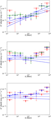 |
Fig. 3 Fermi-LAT SED of the three components included in the best spatial model (Model 6): the H.E.S.S. Top panel: NE limb. Middle panel: point source coincident with the SW limb. Bottom panel: Hα component. For all SEDs, blue error bars represent the statistical uncertainties, while the red ones correspond to the statistical and systematic uncertainties added in quadrature. For upper limits, the two red arrows indicate the extrema of upper limits obtained with the different systematics. The solid and dashed blue lines represent the best spectral fit and its 68% confidence band. For the NE and SW components, the green spectral points indicate the spectra derived for Model 8 using the two radio halves (only statistical errors are presented for better visibility; systematic uncertainties for this model are indicated in Table 3). |
5 Discussion and modelling of the multi-wavelength data
Located 550 pc above the plane (assuming a distance of 2.2 kpc), the SNR SN 1006 evolves in a tenuous environment and its shock velocity exceeds 5000 km s–1 (Katsuda et al. 2009; Winkler et al. 2014). Deep X-ray observations through a dedicated XMM-Newton Large Programme have revealed that the ambient density is ~0.035 cm–3 in the south-eastern (SE) limb (Miceli et al. 2012). Similar estimates have been obtained within the Chandra Large Programme (Winkler et al. 2014; Giuffrida et al. 2022) showing a homogeneous spatial distribution of the ambient medium around SN 1006 in the SE and up to the NE regions. Sano et al. (2022) recently proposed a different description of the circumstellar medium but there exist no indications of shocked gas at those high densities. The tenuous environment surrounding the remnant does not favour the proton–proton interactions to produce the γ-ray emission detected by the LAT, especially in the NE limb. However, Miceli et al. (2014) have revealed a dense atomic cloud interacting with the SW synchrotron rim of SN 1006, where efficient particle acceleration is at work. Our assumption is therefore that the observed giga-electronvolt γ-ray emission in the NE is dominated by the inverse Compton (IC) emission of accelerated electrons, explaining the excellent correlation between the X-ray synchrotron emission, the tera-electronvolt emission detected by H.E.S.S., and the signal detected by the LAT. On the other hand, the emission observed by the LAT in the SW would be mostly of a hadronic nature (proton-proton interactions). This might also be the case in the NW region of the remnant, where a bright Hα filament is detected due to the slowing down of the shock by interaction with dense material. However, the emission detected by the LAT in this region is too faint to provide strong constraints. We shall thus concentrate on the modelling of the two bright NE and SW rims using the spectral points derived in Model 8 (two radio halves), because they are directly comparable to the radio data, and the electrons emitting IC in the giga-electronvolt range and synchrotron in the giga-hertz range have similar energies.
For simplicity, we tried to model each limb separately using identical parameters, except for the density of the medium, to determine whether the increase in density in the SW could explain the different emission detected by Fermi. To this aim, we used the radio (Allen et al. 2001) and X-ray (Bamba et al. 2008) data from the whole remnant. At radio energies, we estimated the fraction of the flux in each component to be ≈50% of the whole SNR flux using observations from the GLEAM survey. Doing the same for the X-ray synchrotron flux between 2.5 and 7 keV, we derived a fraction of 57% of the whole SNR flux in the NE component and 43% in the SW part. We used these fractions in our modelling of each component. We also took into account the tera-electronvolt emission detected in the NE and SW limbs by H.E.S.S. (Acero et al. 2010).
In each limb, we adopted the simplest possible assumption that all emission originates from a single population of accelerated protons and electrons contained in a region characterised by a constant matter density and magnetic field strength. The particle spectra were assumed to follow a power law with an exponential cut-off, dN/dE ∝ ηe,pE–Γ exp(–E/Emax), with the same injection index for both electrons and protons set at 2.2 to reproduce the radio spectral index of ≈0.6. The cut-off energies for electrons and protons are different, allowing for a lower energy cut-off for electrons due to synchrotron losses. The radiative models from the naima packages (Zabalza 2015) were used with the Pythia8 parametrisation of Kafexhiu et al. (2014) for the πo decay. In each limb, we assumed an electron-to-proton ratio of Kep = ηe/ηp = 0.01 and a distance of 2.2 kpc. One should note that our model assumes simple diffuse shock acceleration, though Cristofari & Blasi (2019) have demonstrated that re-acceleration of particles at SNR shocks can play a significant role, especially at low gas density. That would change our modelling little because re-acceleration predicts the same spectral slope for electrons and protons.
Modelled SEDs are presented in Figure 4 and their associated parameters are given in Table 4. While the chosen parameters are not unique in their ability to fit the broadband spectrum, they are compatible with those considered in previous works (Acero et al. 2015; Xing et al. 2016) and they demonstrate that the difference in spectrum and morphology detected in the SW limb by the LAT could well be explained by a simple difference in density from an average value of 0.035 cm–3 in the NE to 0.35 cm–3 in the SW. In this case, the total energy transferred to accelerated protons is of the order of 2.6 × 1049 erg. This energy is concentrated in the limbs and would amount to 13% of the kinetic energy, assuming a volume factor of 20% and an explosion energy of 1051 erg. This is consistent with previous estimates in the limbs by Giuffrida et al. (2022) and with the value derived for the historical supernova Kepler (Acero et al. 2022). Our new LAT analysis and simple modelling thus confirms the magnetohydrodynamic simulations performed by Miceli et al. (2016). However, if the SW limb is dominated by gamma rays generated by proton-proton interaction, one would expect a correlation with the density of the medium and more precisely with the atomic cloud detected by Miceli et al. (2014). This does not seem to be the case here, though more statistics would be needed to characterise the morphology of the southwestern emission detected by the LAT. Similarly, we note some hint of a possible double-peaked feature in the SW spectrum, which is not statistically significant. More statistics with the LAT but also at tera-electronvolt energies with the future Cherenkov Telescope Array Observatory (CTAO) would be needed to confirm this effect. One can note that the modelling proposed here is in good agreement with the mixed scenario discussed in Xing et al. (2019). They found that the contribution of the leptonic component is only <30% lower than that of their purely leptonic model and that ~2% of the kinetic energy of the SNR was converted into hadrons to fit the multi-wavelength data of the SW limb. In our case as well, the gamma-ray emission is dominated by the leptonic component above a few giga-electronvolt and the hadronic component only dominates at low energy.
Since the cut-off energy for protons cannot be constrained with the current multi-wavelength data, two different values (20 TeV and 200 TeV) were tested for the SW limb in which γ- ray emission produced by proton-proton interaction is enhanced due to the higher density. As can be seen in Figure 4, an observation time larger than 50 hours will be needed for CTAO6 to be able to constrain the high-energy cut-off of the accelerated protons. In both limbs, the magnetic field value was set at 30 µG, constrained by the X-ray to TeV flux ratio. This value is well below the magnetic field value required to explain the very thin X-ray filaments in the NE rim of SN 1006 (Long et al. 2003). In addition, while our simple one-zone model can account for the measured γ-ray flux, it fails to reproduce the highest-energy spectral points detected by H.E.S.S. in the NE limb, which are higher than the expectations from the IC process, as was already noted by Acero et al. (2010). Such precise modelling at the highest energies would require one to derive the X-ray spectrum of the exact same region analysed with Fermi-LAT. Thanks to the careful scaling performed here on the X-ray spectrum of the whole SNR, we do not expect significant differences in the main parameters of the modelling, except for the maximum energy of the accelerated electrons.
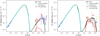 |
Fig. 4 Spectral energy modelling of the NE (left) and SW (right) regions of SN 1006. For all experiments except Fermi, only statistical errors are shown. Modelling parameters are listed in Table 4. The cyan and green lines represent the synchrotron emission and the IC emission, respectively. The black and red dotted lines represent the total and pion decay emission derived for a proton energy cut-off at 200 TeV while the solid ones are derived for 20 TeV. The dashed yellow line indicates the sensitivity of CTA for 50 hours of observation (latest response function: Southern array Prod 5). The blue radio (Allen et al. 2001) and green X-ray (Bamba et al. 2008) data from the whole SNR have been scaled for each limb (see Section 5 for more details). The H.E.S.S. spectral points for each limb (Acero et al. 2010) are indicated in purple. The data points derived in this analysis for the NE and SW limbs are presented in red. |
List of parameters obtained from the modelling of the SED in the NE and SW limbs.
6 Conclusion
By using 15 years of Fermi-LAT data and a summed likelihood analysis with the PSF event types, we were able to perform a complete morphological study of the gamma-ray emission of the SNR SN 1006. We significantly detected both the NE and SW rims of the SNR with TS values of 40 (6σ for 2 d.o.f.) and 34 (5.5σ for 2 d.o.f.), respectively, using radio templates using GLEAM survey data from MWA observations. Additionally, our analysis reveals a 3σ excess coincident with the bright NW Hα filament. We can confirm the harder spectrum of the NE rim with respect to the SW rim. This asymmetry can be reproduced well with a simple one-zone model in which the only difference is the gas density an order of magnitude higher in the SW than in the NE, enhancing the gamma-ray emission produced by proton-proton interaction in the SW especially below a few giga-electronvolt. In contrast, the gamma-ray emission in the NE is dominated by accelerated electrons radiating through IC processes. Assuming a gas density of 0.035 cm−3 in the NE to 0.35 cm−3 in the SW, the total energy transferred to accelerated protons is of the order of 2.6 × 1049 erg. While the cut-off energy is well constrained, especially by X- ray data, an observation time of more than 50 hours would be needed for the future Cherenkov Telescope Array Observatory to be able to constrain the high-energy cut-off of the accelerated protons.
Acknowledgements
The Fermi LAT Collaboration acknowledges generous ongoing support from a number of agencies and institutes that have supported both the development and the operation of the LAT as well as scientific data analysis. These include the National Aeronautics and Space Administration and the Department of Energy in the United States, the Commissariat à l’Energie Atom- ique and the Centre National de la Recherche Scientifique/Institut National de Physique Nucléaire et de Physique des Particules in France, the Agenzia Spaziale Italiana and the Istituto Nazionale di Fisica Nucleare in Italy, the Ministry of Education, Culture, Sports, Science and Technology (MEXT), High Energy Accelerator Research Organization (KEK) and Japan Aerospace Exploration Agency (JAXA) in Japan, and the K. A. Wallenberg Foundation, the Swedish Research Council and the Swedish National Space Board in Sweden. Additional support for science analysis during the operations phase is gratefully acknowledged from the Istituto Nazionale di Astrofisica in Italy and the Centre National d’Études Spatiales in France. This work performed in part under DOE Contract DE-AC02-76SF00515. M.L.G. acknowledges support from the Alexander von Humboldt Foundation and from ANR for the GAMALO project under reference ANR-19-CE31-0014. Softwares: This research made use of the Python package fermipy for the Fermi-LAT analysis (Wood et al. 2017). The naima package was used for the modelling (Zabalza 2015).
Appendix A Fermi-LAT angular resolution
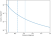 |
Fig. A.1 Fermi-LAT radial distribution of photons from a point source simulated with a spectral index of 2.0 between 1 GeV and 1 TeV, presented with a solid line. The dashed, dotted-dashed and dotted lines indicate the Half-Width at Half Maximum, the 50% and 68% containment radii, respectively. |
As already discussed in the main text, the angular resolution of the LAT depends strongly on the gamma-ray’s energy. Above 1 GeV, the PSF improves drastically, with a 68% containment radius smaller than 0.2° above 10 GeV. To better understand how this performance is characterised in our energy interval of interest (1 GeV—1 TeV for the morphological analysis in Section 3), we simulate a point source with a spectral index of 2.0 as a compromise between the hard component in the NE of the remnant and the softer component in the SW. Figure A.1 shows the distribution of photons from this point source and the associated performances between 1 GeV and 1 TeV: the Half-Width at Half Maximum (HWHM) of 0.05°, which contains 13% of photons in our case, the R50 (Half-Energy Width) of 0.25° and the R68 (68% containment radius) of 0.43°. The LAT PSF is quite peaked but still contains large tails of photons as can be seen in this Figure.
References
- Acero, F., Aharonian, F., Akhperjanian, A. G., et al. 2010, A&A, 516, A62 [NASA ADS] [CrossRef] [EDP Sciences] [Google Scholar]
- Acero, F., Lemoine-Goumard, M., Renaud, M., et al. 2015, A&A, 580, A74 [NASA ADS] [CrossRef] [EDP Sciences] [Google Scholar]
- Acero, F., Ackermann, M., Ajello, M., et al. 2016, ApJS, 224, 8 [NASA ADS] [CrossRef] [Google Scholar]
- Acero, F., Lemoine-Goumard, M., & Ballet, J. 2022, A&A, 660, A129 [NASA ADS] [CrossRef] [EDP Sciences] [Google Scholar]
- Ackermann, M., Ajello, M., Albert, A., et al. 2012, ApJS, 203, 4 [Google Scholar]
- Akaike, H. 1998, Information Theory and an Extension of the Maximum Likelihood Principle, eds. E. Parzen, K. Tanabe, & G. Kitagawa (New York, NY: Springer), 199 [Google Scholar]
- Allen, G. E., Petre, R., & Gotthelf, E. V. 2001, ApJ, 558, 739 [NASA ADS] [CrossRef] [Google Scholar]
- Araya, M., & Frutos, F. 2012, MNRAS, 425, 2810 [NASA ADS] [CrossRef] [Google Scholar]
- Atwood, W. B., Abdo, A. A., Ackermann, M., et al. 2009, ApJ, 697, 1071 [CrossRef] [Google Scholar]
- Bamba, A., Fukazawa, Y., Hiraga, J. S., et al. 2008, PASJ, 60, S153 [NASA ADS] [Google Scholar]
- Bruel, P., Burnett, T. H., Digel, S. W., et al. 2018, Fermi-LAT improved Pass 8 event selection [Google Scholar]
- Condon, B., Lemoine-Goumard, M., Acero, F., & Katagiri, H. 2017, ApJ, 851, 100 [NASA ADS] [CrossRef] [Google Scholar]
- Cristofari, P., & Blasi, P. 2019, Mon. Not. Roy. Astron. Soc., 489, 108 [CrossRef] [Google Scholar]
- Giuffrida, R., Miceli, M., Caprioli, D., et al. 2022, Nat. Commun., 13, 5098 [NASA ADS] [CrossRef] [Google Scholar]
- Hurley-Walker, N., Callingham, J. R., Hancock, P. J., et al. 2017, MNRAS, 464, 1146 [Google Scholar]
- Kafexhiu, E., Aharonian, F., Taylor, A. M., & Vila, G. S. 2014, Phys. Rev. D, 90, 123014 [Google Scholar]
- Katsuda, S., Petre, R., Long, K. S., et al. 2009, ApJ, 692, L105 [NASA ADS] [CrossRef] [Google Scholar]
- Koyama, K., Petre, R., Gotthelf, E. V., et al. 1995, Nature, 378, 255 [Google Scholar]
- Li, J.-T., Ballet, J., Miceli, M., et al. 2018, ApJ, 864, 85 [CrossRef] [Google Scholar]
- Long, K. S., Reynolds, S. P., Raymond, J. C., et al. 2003, ApJ, 586, 1162 [Google Scholar]
- Miceli, M., Bocchino, F., Decourchelle, A., et al. 2012, A&A, 546, A66 [NASA ADS] [CrossRef] [EDP Sciences] [Google Scholar]
- Miceli, M., Acero, F., Dubner, G., et al. 2014, ApJ, 782, L33 [NASA ADS] [CrossRef] [Google Scholar]
- Miceli, M., Orlando, S., Pereira, V., et al. 2016, A&A, 593, A26 [NASA ADS] [CrossRef] [EDP Sciences] [Google Scholar]
- Sano, H., Yamaguchi, H., Aruga, M., et al. 2022, ApJ, 933, 157 [NASA ADS] [CrossRef] [Google Scholar]
- Winkler, P. F., Gupta, G., & Long, K. S. 2003, ApJ, 585, 324 [Google Scholar]
- Winkler, P. F., Williams, B. J., Reynolds, S. P., et al. 2014, ApJ, 781, 65 [NASA ADS] [CrossRef] [Google Scholar]
- Wood, M., Caputo, R., Charles, E., et al. 2017, in 35th International Cosmic Ray Conference (ICRC2017), 301, 824 [Google Scholar]
- Xing, Y., Wang, Z., Zhang, X., & Chen, Y. 2016, ApJ, 823, 44 [NASA ADS] [CrossRef] [Google Scholar]
- Xing, Y., Wang, Z., Zhang, X., & Chen, Y. 2019, PASJ, 71, 77 [NASA ADS] [CrossRef] [Google Scholar]
- Zabalza, V. 2015, in 34th International Cosmic Ray Conference (ICRC2015), 922 [Google Scholar]
The energy dispersion correction is applied to all sources in the model, except for the isotropic diffuse emission model. More details can be found in the FSSC: https://fermi.gsfc.nasa.gov/ssc/data/analysis/documentation/Pass8_edisp_usage.html
The sensitivities for CTAO are available at https://www.ctao.org/for-scientists/performance/
All Tables
Results of the fit of the LAT data between 1 GeV and 1 TeV using different spatial models.
Fermi-LAT morphological parameters of the three sources in Model 6 and two sources in Model 8 derived between 1 GeV and 1 TeV.
Fermi-LAT spectral parameters of the components in Model 6 and Model 8 between 100 MeV and 1 TeV.
List of parameters obtained from the modelling of the SED in the NE and SW limbs.
All Figures
|
Fig. 1 Fermi-LAT TS map above 1 GeV for the 1.5° × 1.5° region around the SNR SN 1006. The black cross indicates the only 4FGL- DR4 source in the region (4FGL J1503.6–4146), while the magenta cross indicates the point source coincident with the SW rim added in our best model. The cyan contours represent the H.E.S.S. significance contours at 3, 5, and 7σ (Acero et al. 2010). White contours show the Hα template generated from the 4m Blanco telescope observations at CTIO (Winkler et al. 2014). Yellow contours present the radio spatial template derived using observations from the Murchison Widefield Array (Hurley-Walker et al. 2017). The inset on the bottom left corner provides the counts map from a simulated point source in the same coordinate system (more details in Appendix A). |
| In the text | |
|
Fig. 2 Fermi-LAT TS map above 1 GeV after removing one of the three components from the best spatial model (Model 6, see Table 1): the H.E.S.S. NE limb (top panel), the Point source in the SW (middle panel), and the Hα component (bottom panel) with a reduced colour scale. For all TS maps, we present the 1.5° × 1.5° ROI around SN 1006. The cyan contours represent the H.E.S.S. significance contours at 3, 5, and 7σ (Acero et al. 2010). White contours show the Hα template used in our analysis. |
| In the text | |
|
Fig. 3 Fermi-LAT SED of the three components included in the best spatial model (Model 6): the H.E.S.S. Top panel: NE limb. Middle panel: point source coincident with the SW limb. Bottom panel: Hα component. For all SEDs, blue error bars represent the statistical uncertainties, while the red ones correspond to the statistical and systematic uncertainties added in quadrature. For upper limits, the two red arrows indicate the extrema of upper limits obtained with the different systematics. The solid and dashed blue lines represent the best spectral fit and its 68% confidence band. For the NE and SW components, the green spectral points indicate the spectra derived for Model 8 using the two radio halves (only statistical errors are presented for better visibility; systematic uncertainties for this model are indicated in Table 3). |
| In the text | |
|
Fig. 4 Spectral energy modelling of the NE (left) and SW (right) regions of SN 1006. For all experiments except Fermi, only statistical errors are shown. Modelling parameters are listed in Table 4. The cyan and green lines represent the synchrotron emission and the IC emission, respectively. The black and red dotted lines represent the total and pion decay emission derived for a proton energy cut-off at 200 TeV while the solid ones are derived for 20 TeV. The dashed yellow line indicates the sensitivity of CTA for 50 hours of observation (latest response function: Southern array Prod 5). The blue radio (Allen et al. 2001) and green X-ray (Bamba et al. 2008) data from the whole SNR have been scaled for each limb (see Section 5 for more details). The H.E.S.S. spectral points for each limb (Acero et al. 2010) are indicated in purple. The data points derived in this analysis for the NE and SW limbs are presented in red. |
| In the text | |
|
Fig. A.1 Fermi-LAT radial distribution of photons from a point source simulated with a spectral index of 2.0 between 1 GeV and 1 TeV, presented with a solid line. The dashed, dotted-dashed and dotted lines indicate the Half-Width at Half Maximum, the 50% and 68% containment radii, respectively. |
| In the text | |
Current usage metrics show cumulative count of Article Views (full-text article views including HTML views, PDF and ePub downloads, according to the available data) and Abstracts Views on Vision4Press platform.
Data correspond to usage on the plateform after 2015. The current usage metrics is available 48-96 hours after online publication and is updated daily on week days.
Initial download of the metrics may take a while.