| Issue |
A&A
Volume 591, July 2016
|
|
|---|---|---|
| Article Number | A34 | |
| Number of page(s) | 11 | |
| Section | Stellar atmospheres | |
| DOI | https://doi.org/10.1051/0004-6361/201628453 | |
| Published online | 07 June 2016 | |
ζ2 Reticuli, its debris disk, and its lonely stellar companion ζ1 Ret
Different Tc trends for different spectra⋆,⋆⋆
1
Instituto de Astrofísica e Ciências do Espaço, Universidade do
Porto, CAUP, Rua das
Estrelas, 4150-762
Porto,
Portugal
e-mail:
Vardan.Adibekyan@astro.up.pt
2
Departamento de Física e Astronomia, Faculdade de Ciências,
Universidade do Porto, Rua do Campo
Alegre, 4169-007
Porto,
Portugal
3
Instituto de Astrofísica de Canarias, 38200, La Laguna, Tenerife, Spain
4
Departamento de Astrofísica, Universidad de La
Laguna, 38206, La
Laguna, Tenerife,
Spain
5
Leibniz Institute for Astrophysics Potsdam (AIP),
An der Sternwarte 16,
14482
Potsdam,
Germany
6
Byurakan Astrophysical Observatory, 0213 Byurakan, Aragatsotn province,
Armenia
Received: 7 March 2016
Accepted: 24 April 2016
Context. Several studies have reported a correlation between the chemical abundances of stars and condensation temperature (known as Tc trend). Very recently, a strong Tc trend was reported for the ζ Reticuli binary system, which consists of two solar analogs. The observed trend in ζ2 Ret relative to its companion was explained by the presence of a debris disk around ζ2 Ret.
Aims. Our goal is to re-evaluate the presence and variability of the Tc trend in the ζ Reticuli system and to understand the impact of the presence of the debris disk on a star.
Methods. We used very high-quality spectra of the two stars retrieved from the HARPS archive to derive very precise stellar parameters and chemical abundances. We derived the stellar parameters with the classical (nondifferential) method, while we applied a differential line-by-line analysis to achieve the highest possible precision in abundances, which are fundamental to explore for very tiny differences in the abundances between the stars.
Results. We confirm that the abundance difference between ζ2 Ret and ζ1 Ret shows a significant (~2σ) correlation with Tc. However, we also find that the Tc trends depend on the individual spectrum used (even if always of very high quality). In particular, we find significant but varying differences in the abundances of the same star from different individual high-quality spectra.
Conclusions. Our results for the ζ Reticuli system show, for example, that nonphysical factors, such as the quality of spectra employed and errors that are not accounted for, can be at the root of the Tc trends for the case of individual spectra.
Key words: stars: abundances / planetary systems / stars: individual: Zet1 Ret (HD 20766) / techniques: spectroscopic / stars: individual: Zet2 (HD 20807) / binaries: general
Based on data obtained from the ESO Science Archive Facility under request number vadibekyan204818, vadibekyan204820, and vadibekyan185979.
The tables with EWs of the lines and chemical abundances are only available at the CDS via anonymous ftp to cdsarc.u-strasbg.fr (130.79.128.5) or via http://cdsarc.u-strasbg.fr/viz-bin/qcat?J/A+A/591/A34
© ESO, 2016
1. Introduction
In the last decade, noticeable advances were made in the characterization of atmospheric properties and chemical compositions of cool, sun-like stars. The achieved high precision in chemical abundances allowed observers to study the chemical abundances of stars with and without planets in detail (e.g., Gilli et al. 2006; Robinson et al. 2006; Delgado Mena et al. 2014, 2015; Kang et al. 2011; Adibekyan et al. 2012a,b, 2015c). These studies are very important since the chemical abundances of stars with planets provide a huge wealth of information about the planet formation process (e.g., Bond et al. 2010; Delgado Mena et al. 2010), composition of planets (e.g., Thiabaud et al. 2014; Dorn et al. 2015; Santos et al. 2015), and even about the habitability of the planets (e.g., Adibekyan et al. 2015a).
The achieved extremely high precision in chemical abundances also facilitated the study of very subtle chemical peculiarities in stars that had initially appeared to be Sun-like. The quintessential example, the so-called Tc trend, is the trend of individual chemical abundances with the condensation temperature (Tc) of the elements. Many studies, beginning with Gonzalez (1997) and Smith et al. (2001), attempted to search for planet accretion and/or formation signatures in the photospheric chemical compositions of cool stars by looking at the Tc trends (e.g., Takeda et al. 2001; Ecuvillon et al. 2006; Sozzetti et al. 2006; Meléndez et al. 2009; Ramírez et al. 2009; González Hernández et al. 2010, 2013; Schuler et al. 2011b; Maldonado et al. 2015; Nissen 2015; Biazzo et al. 2015; Saffe et al. 2015).
Meléndez et al. (2009) claimed that the Sun shows a deficiency in refractory elements with respect to other solar twins because these elements were trapped in the terrestrial planets in our solar system. The same conclusion was also reached by Ramírez et al. (2009), who analyzed 64 solar twins and analogs with and without detected planets. However, later results by González Hernández et al. (2010) and González Hernández et al. (2013) strongly challenge the relation between the presence of planets and the abundance peculiarities of the stars.
Rocky material accretion is by far not the only explanation for the Tc trend. Recently, Adibekyan et al. (2014) showed that the Tc trend strongly depends on the stellar age1 and they found a tentative dependence on the galactocentric distances of the stars. The authors concluded that the Tc trend depends on the Galactic chemical evolution (GCE) and suggested that the difference in Tc slopes, observed between planet hosting solar analogs and solar analogs without detected planets, may reflect their age difference. Maldonado et al. (2015) and Maldonado & Villaver (2016) also confirmed the correlation of the Tc trend with age, and further suggested a significant correlation with the stellar radius and mass. Önehag et al. (2014) in turn showed that while the Sun shows a different Tc trend when compared to the solar-field twins, it shows a very similar abundance trend with Tc when compared to the stars from the open cluster M 67. These authors suggested that the Sun, unlike most stars, was formed in a dense stellar environment where the protostellar disk was already depleted in refractory elements before the star formation. Gaidos (2015) also suggested that gas-dust segregation in the disk can be responsible for the Tc trends.
While above mentioned mechanisms and processes (e.g., GCE or age effect) can be responsible for the general Tc trends for field-star samples, they cannot easily explain trends observed between companions of binary systems. Several authors studied the Tc trend in binary stars with and without planetary companions (e.g., Liu et al. 2014; Saffe et al. 2015; Mack et al. 2016) or binary stars where both components host planets (e.g., Biazzo et al. 2015; Teske et al. 2015, 2016; Ramírez et al. 2015). The results and conclusions of these studies show that there are no systematic differences in the chemical abundances of stars with and without planets in binary systems. Moreover, there is no consensus on the results even for the same, individual systems (e.g., 16 Cyg AB; Laws & Gonzalez 2001; Takeda 2005; Schuler et al. 2011a; Tucci Maia et al. 2014).
Recently, Maldonado et al. (2015) studied a large sample of stars with and without debris disks to search for chemical anomalies related to the formation of planets. They found no significant differences in chemical abundances or in the Tc trends between the two samples. However, very recently, Saffe et al. (2016,hereafter S16) reported a positive Tc trend in the binary system, ζ1 Ret – ζ2 Ret, where one of the stars (ζ2 Ret) hosts a debris disk. The authors explained the deficit of the refractory elements relative to volatiles in ζ2 Ret as caused by the depletion of about ~3 M⊕ rocky material.
The two stars have very similar atmospheric parameters, which in principle allows for a very high-precision relative abundance characterization of the stars. Taking full advantage of this, S16 carried out a detailed and careful analysis of the system. However, the authors chose to use only the spectra of the stars observed during the same night with the same instrument (High Accuracy Radial velocity Planet Searcher – HARPS). The final signal-to-noise ratio (S/N) of the spectra that they used was ~300 (S16), while we noticed that much higher S/N (see Table 1) can be achieved if all of the spectra from the European Southern Observatory HARPS (ESO) archive2 are combined. Moreover, some of the individual spectra found in the archive have S/N of more than 350, which allows us to carry out a differential abundance analysis between different spectra of the same star, which in turn provides an independent estimation of the precision of our measurements.
This case motivated us to explore whether the observed differences in the chemical abundances of the stars could be simply due to some systematics in the spectra. In this work, we use very high-quality spectra of the ζ1 Ret and ζ2 Ret binary star system to re-evaluate the presence and variability of the Tc trend in this system and, as such, better understand the impact of the presence of the debris disk on a star. We organized this paper as follows. In Sect. 2 we present the data, in Sect. 3 we present the methodology used to derive the stellar parameters and chemical abundances, and in Sect. 4 we explain how we calculate and evaluate the significance of the Tc trends. After presenting the main results in Sect. 5, we conclude in Sect. 6.
Stellar parameters, S/N, and observation dates of ζ1 Ret and ζ2 Ret derived from individual and combined spectra.
2. Data
Both stars of this binary system were extensively observed with the HARPS high-resolution spectrograph (Mayor et al. 2003) at the 3.6 m telescope (La Silla Paranal Observatory, ESO). The HARPS archive contains ~70 and ~170 spectra for ζ1 Ret and ζ2 Ret, respectively. We use the combined spectra of the stars (referred as “starname_comb” in Table 1), spectra that were used in S16 (referred as “starname_S16” in Table 1), and three individual spectra with the highest S/N for each star (referred as “starname_a”, “starname_b”, and “starname_c” in Table 1). The highest S/N spectra are used to provide the final characteristics of this system. The individual high S/N spectra are selected to estimate the internal precision of the methods, while the spectra used by S16 are selected for external comparison.
A few of the spectra of these stars were obtained under poor atmospheric conditions (the headers of the fits files report −1.00 value for seeing), and we considered these spectra unsuitable for this work and, therefore, chose not to use them. These spectra had very low S/N and combining them would increase the total S/N of the combined spectra (listed in Table 1) by 0.03 and 1.6% for ζ1 Ret and ζ2 Ret, respectively. The S/N at the 40th fiber order (central wavelength ~5060 Å) for each of the HARPS spectra (retrieved from the header of the spectra) are presented in Table 13. As one can see, even the individual spectra of the stars have a much higher S/N than that of the spectra used in S16 and, in the combined spectra, the S/N are higher by a factor of about six and ~13 for ζ1 Ret and ζ2 Ret, respectively. We note again that S16 chose to use the spectra of the stars obtained during the same night, probably to minimize the time-dependent systematics. For the Sun, we used a combined HARPS reflected spectrum from Vesta (extracted from the same public archive, S/N ~ 1300).
3. Stellar parameters and chemical abundances
We derived the stellar parameters (Teff, [Fe/H], log g, and Vtur) for the stars from the various spectra and for the Sun with the procedure described in Sousa (2014). In short, we first automatically measured the equivalent widths (EWs) of iron lines (~250 Fe i and ~40 Fe ii lines) using the ARES v2 code4 (Sousa et al. 2015). Then the spectroscopic parameters were derived by imposing excitation and ionization balance assuming LTE (see Fig. 1). We used the grid of ATLAS9 plane-parallel model of atmospheres (Kurucz 1993) and the 2014 version of MOOG5 radiative transfer code (Sneden 1973). We derived the parameters of the stars with a classical rather than a line-by-line differential approach. In general, when stars with similar stellar parameters are compared, the two methods give very similar results and the estimated errors in case of differential line-by-line analysis are slightly smaller. The uncertainties of the parameters are derived as in our previous works and they are well described in Neuforge-Verheecke & Magain (1997). The derived stellar parameters are listed in Table 1.
The values in Table 1 show that the stellar parameters of the same stars derived from different spectra agree very well within the estimated errors. Furthermore, when the same spectra are used, our atmospheric parameters agree very well with those derived in S16. In particular, we obtained ΔTeff = 12 K, Δ[Fe/H] = 0.004 dex, Δlog g = −0.03 dex, and ΔVtur = 0.06 km s-1 for ζ1 Ret, where the differences are defined as our values minus those of S16. For ζ2 Ret, the differences are ΔTeff = −21 K, Δ[Fe/H] = −0.003 dex, Δlog g = −0.06 dex, and ΔVtur = 0.00 km s-1.
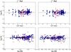 |
Fig. 1 Iron abundance vs. excitation potential (upper panels) and iron abundance vs. reduced EW (lower panels) for ζ1 Ret_comb and ζ2 Ret_comb. The blue and red symbols correspond to the neutral and ionized iron lines. The black solid line indicates the linear fit of the data. |
Similar to S16, we derived 0.027 dex higher metallicity for ζ1 Ret compared to ζ2 Ret with the same spectra. However, the difference decreases to 0.009 dex when the spectra with the highest S/N ratio are considered. Also, when different pairs of spectra of the stars are compared, the maximum difference is obtained when the ζ1 Ret_S16 and ζ2 Ret_S16 are used, and when ζ1 Ret_comb and ζ2 Ret_a pairs are compared, the ζ2 Ret appears even slightly more metal rich than ζ1 Ret by −0.001 dex. These results suggest that one should be cautious when reaching such an extremely small difference in stellar parameters.
Elemental abundances for the stars were also determined using an LTE analysis and the same tools and codes as for stellar parameters determination. We adopted the initial line list for Na, Mg, Al, Si, Ca, Ti, Cr, Ni, Co, Sc, Mn, and V from Adibekyan et al. (2012c), but several lines (two Si i lines λ5701.11, λ6244.48, two Ca i lines λ5261.71, λ5352.05, three Ti i lines λ4722.61, λ5039.96, λ5965.84, one Ti ii line λ 5381.03, two Cr i lines λ5122.12, λ6882.52, and two Ni i lines λ5081.11, λ6767.78) were excluded because of large [X/Fe] star-to-star scatter at solar metallicities (Adibekyan et al. 2015b). Finally, Ni i line at λ6360.81 was excluded because of unreliable EW measurements (because of a depressed continuum) and the Sc i line at λ5520.50 was excluded because there is no data about the hyperfine structure splitting (HFS) of the lines in Kurucz atomic line database6 nor in Prochaska et al. (2000), which are our two sources for the relative log gf values.
We determined oxygen abundances using two weak lines at 6158.2 Å and 6300.3 Å following the work of Bertran de Lis et al. (2015), although it was only possible to measure the 6158.2 Å lines for the combined spectra of ζ1 Ret and ζ2 Ret and for the three individual spectra of ζ2 Ret. Sulfur abundances were calculated by performing spectral synthesis with MOOG around the lines 6046.0 Å, 6052.5 Å, 6743.5Å, and 6757.1 Å. The atomic data of those lines and the surrounding lines were taken from VALD3 database7. The lines at 6046.0 Å and 6052.5 Å (used in S16) suffer from non-negligible blends of CN bands, thus, our initial abundances derived from EWs yielded higher abundances than the other two lines. To fit the lines in the solar spectra, we had to calibrate the log gfs of the S lines (the line list and atomic data are available at the CDS), to match a solar sulfur abundance A(S) = 7.16 (Asplund et al. 2009). Cerium abundances were derived using the three spectral lines presented in Reddy et al. (2003) and the line at 5274.2 Å for which the atomic data was extracted from VALD3. Carbon abundances were based on the two well-known CI optical lines at 5052 Å and 5380 Å. The atomic data for carbon and elements heavier than Ni were also extracted from VALD3 (a more detailed line list will be shown in Delgado Mena et al., in prep).
When available, the Barklem damping van der Waals constants were used for all of the elements. Otherwise, the Unsöld approximation multiplied by a factor (1.0 + 0.67 × E.P., where E.P. is the excitation potential of a line) suggested by the Blackwell group was used (option 2 in the damping parameter inside MOOG). For the Sc, V, Mn, Co, Cu, and Ba lines, HFS was considered. We adopted the atomic parameters and isotopic ratios from Prochaska et al. (2000) for Ba, and the relative log gf values and isotopic ratios for the lines were taken from Kurucz database for the remaining elements.
The EWs of the lines were derived with ARES v2 code, but with careful visual inspection. In a few cases, when the ARES measurements were not satisfactory (this can happen, e.g., as a result of a presence of cosmic rays or bad pixels), we measured the EWs using the task splot in IRAF8. We calculated the final abundance of the elements (when several spectral lines were available) as a weighted mean of all of the abundances, where the distance from the median abundance was considered as a weight. As demonstrated in Adibekyan et al. (2015b), this method can be effectively used without removing suspected outlier lines.
We performed differential line-by-line analysis relative to the Sun for the combined and S16 spectra. We also performed differential abundance analysis of ζ2 Ret_comb relative to ζ1 Ret_comb, and ζ2 Ret_S16 relative to ζ1 Ret_S16. Finally, for both stars we derived differential abundances from each of the individual three spectra (“starname_b” and “starname_c” relative to “starname_a”) relative to each other.
The errors of the [X/H] abundances are calculated as a quadrature sum of the errors due to EW measurements and errors due to uncertainties in the atmospheric parameters. When three or more lines were available, the EW measurement error is estimated as σ/ , where σ is the line-to-line abundance scatter and n is the number of the observed lines. The errors arising from uncertainties in the stellar parameters are calculated as a quadratic sum of the abundance sensitivities on the variation of the stellar parameters by their one σ uncertainties. These errors are usually much smaller (because of very small uncertainties in stellar parameters) than the errors due to EW measurements.
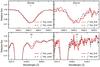 |
Fig. 2 Spectral regions containing oxygen lines in ζ1 Ret_comb, ζ2 Ret_comb, ζ1 Ret_S16, and ζ2 Ret_S16 spectra. |
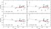 |
Fig. 3 Differential abundances [X/H] against condensation temperature for ζ1 Ret and ζ2 Ret. The abundances are derived relative to the Sun with the combined spectra and spectra from S16. The black dashed line represents the trend when all of the elements are used for the linear regression and the red line is the result of the linear regression when only elements with Tc> 900 K are used. |
The error estimation method described in the previous paragraph is most frequently used, even when only two lines are observed. However, the dispersion (σsample) calculated using only two lines can be very different from the dispersion rooted in the uncertainty on the abundances, a value that can only be efficiently estimated if large number of lines are available. A simple calculation shows that if one assumes that the errors follow a normal distribution and that σsample is the standard deviation of that distribution, then the σtwo−lines calculated from two random lines from that distribution peaks close to zero, underestimating σsample. The σtwo−lines is smaller than 0.5σreal in ~38% cases and σtwo−lines is five times smaller than σreal in ~16% cases. Moreover, in the cases when two lines of an element give exactly the same abundance, then the calculated dispersion is zero and the final error is equal to the error due to uncertainties in the atmospheric parameters. Since the latter is usually very small, the weight given to this element when calculating the Tc slope is extremely high (see Sect. 4). Such underestimated errors can play a crucial role in the incorrect determination of the slopes.
We calculated the errors on EWs following Cayrel (1988) to provide more realistic errors for the abundances of elements that only have two observed spectral lines in our spectra (except oxygen) . The calculated uncertainty takes into account the statistical photometric error due to the noise in each pixel and the error related to the continuum placement, which is the dominant contribution to the error (Cayrel 1988; Bertran de Lis et al. 2015). Then, these errors are propagated to derive the abundance uncertainties for each line. The final uncertainties for the average abundance are propagated from these individual errors.
When only one line for a given element is available, as is the case for O (for some spectra) and Sr, we determine the error by measuring a second EW with the position of the continuum displaced within the root mean square (rms) due to the noise of the spectra, and calculating the difference in abundance with respect to the original value. In this manner, the elements with only a weak line (as for oxygen in some cases) have a large error in their abundance measurements. This is in contrast to elements with strong lines, such as Sr, where the fact of having a single line does not affect the final error too much; see, for comparison, the error bars in Fig. 3 for O and Sr and how they vary between the highest and lowest S/N spectra). We stress here the case of oxygen for which we find a very different value than S16. Their differential abundance (ζ1 Ret – ζ2 Ret) is almost 0.1 dex lower than ours and their reported error is much smaller. In Fig. 2 we show a part of the spectra used by S16 around the 6300 Å region; it is strongly affected by noise. The EW values are very similar for both stars, but our abundance determinations have a larger error because of the strong effect of a small change in the continuum in this very weak line. As mentioned by S16, this line is blended with a Ni line, and if we consider that the two stars have similar Ni abundances, it seems difficult to reconcile such a large difference in abundance values even if our atomic parameters for the Ni blend are different. However, for the combined, very high S/N spectra we can also measure with better precision the oxygen line at 6158.2 Å, which suggests very similar oxygen abundance to that derived from the 6300.3 Å line. This example shows the difficulty in measuring oxygen abundances. Such an issue is very important in the context of Tc trend analysis, as the low condensation temperature of oxygen leads to a strong leverage on the final slope value.
Since both oxygen lines are very weak and deserve special attention (see, e.g., Bertran de Lis et al. 2015), even when both lines were observed for a spectrum we calculated individual errors for each line (as described in the previous paragraph) and then propagated the error of the average oxygen abundance. The EWs of all of the measured lines and the abundances of the elements derived from all of the spectra are available on the CDS.
4. Tc slope
Once the differential abundances and corresponding errors are derived we can search for abundance trends with the condensation temperature of the elements. The 50% Tc equilibrium condensation temperatures for a gas of solar system composition are taken from Lodders (2003). It is common practice to plot [X/Fe] (and not just [X/H]) versus Tc, which allows us to remove the trends related to Galactic chemical evolution (e.g., González Hernández et al. 2013; Saffe et al. 2016). Although this procedure can be justified when stars with different metallicities are compared, it can produce a bias in the derived slope. Subtracting the iron abundance (a constant value) from each elemental abundance should only shift the trend but should not change the slope. However, since iron abundance has an error itself, the propagated errors of the [X/Fe] abundance ratios should be adjusted. This change in turn can have an impact on the original slope. In an extreme (although not very realistic) case that the error of iron abundance is much larger than the errors of individual [X/H] abundances, then the propagated errors of [X/Fe] abundance ratios would be dominated by the error of [Fe/H]. In this case the weighted least-squares regression would give a result similar to an ordinary least-squares regression, i.e., the weights of all of the elements would be similar. This discussion suggests that if the abundances are normalized to another element (not iron), the result would be different depending on the error of the element used for normalization. Moreover, if the abundances are not normalized to the iron abundance, the [Fe/H] value can also be used in the calculations of the slopes. For these reasons we use [X/H] in our analysis when deriving the Tc trend.
Slopes of the [X/H] vs. Tc for different pairs of spectra.
In Table 2 we present the Tc slopes, corresponding standard errors, 95% confidence intervals (CI) and p-values (at α = 0.05 significance level). The Tc slopes refer to the slope of the linear dependence between [X/H] and Tc. We calculated the slopes with the weighted least-squares (WLS) technique, whereas we calculated the weights as the inverse of the variance (σ2) of the abundance. The p-values come from the F-statistics that tests the null hypothesis that the data can be modeled accurately by setting the regression coefficients to zero. The 95% confidence intervals are calculated using the standard error of the slopes and the p-value from T-statistics that tests the null hypothesis that the coefficient of a predictor variable is zero, i.e., slope is zero.
We also use a Bayesian approach to assess the presence of a dependence of [X/H] on Tc and to calculate the slope of the dependence. It has been shown that p-value analysis, even if very widespread, is not as robust as expected; the assessment of the significance of a correlation is further complicated when the p-value is close to the significance level. In Figueira et al. (2016) we provided a straightforward alternative Bayesian approach to the assessment and characterization of a correlation in a dataset. However, relying on the Pearson correlation coefficient and Sperman’s rank, Figueira et al. (2016) did not consider the impact of error bars on the measurements. We consider the case of a linear regression in which the value of each ordinate Yi follows a Gaussian distribution of center dictated by the evaluation of a linear slope on the abscissa Xi and variance given by σ2. Using the MCMC (Markov Chain Monte Carlo) algorithm implemented in PyMC (Patil et al. 2010), and assuming uninformative Gaussian distributions of center 0 and σ = 1000 as priors for the slope parameters and intersect, we estimated the best fit to the data. In Table 2 we present the Tc slopes and the associated 95% credible intervals (highest posterior density; HPD) calculated by applying this Bayesian approach.
The Bayesian and frequentist analyses differ in important ways. Since both approaches are addressing and solving exactly the same problem, the slopes calculated by the two methods are almost identical. However, since the CI (in frequentist analysis) and the HPD (in Bayesian approach) have different meanings, their values can be different and should be interpreted differently (e.g., Morey et al. 2015). A 95% CI is an interval that in repeated sampling has a 0.95 probability of containing the true value of the parameter, i.e, if a large number of samples are used, the true value of the slope will fall within the CI in 95% of the cases. A 95% HPD is the interval that contains the true value of slope with a probability of 0.95 given the current sample (data). This said, it should not come as a surprise that a 95% HPD is usually much smaller than the 95% CI, which makes most of the correlations significant (at 95% level).
In Table 2 we present the Tc slopes that were derived for different pairs of stars and spectra. The slopes are derived by considering all of the elements and also by considering only refractory elements that have Tc> 900 K.
To understand better how the calculated Tc slopes are sensitive to the abundance uncertainties, we also calculated the slopes without considering the errors. In the frequentist approach giving the same error (which means the same weight) to all of the elements or not considering errors yields the same results, since the calculated slope value is only sensitive to the relative weights of the points. In the Bayesian approach, the absolute error value of each point is important when evaluating the significance of the correlations, i.e., assuming 0.01 dex error for all of the elements produces a result that is very different if an error of 0.1 dex was assumed for all of the elements.
In the Appendix we present all of the Tc trend calculations discussed in the main text, without considering the errors for the individual abundances, i.e., applying an ordinary linear regression (OLS).
5. Results
In Fig. 3 we show the dependence of differential [X/H] abundances of ζ1 Ret and ζ2 Ret relative to the Sun on the corresponding Tc. The abundances are derived using the combined spectra and spectra that were used in S16. Table 2 and the corresponding plot shows that there is no trend with Tc for ζ1 Ret, while ζ2 Ret shows a significant trend when the frequentist p-values are considered for null-hypothesis rejection testing. This trend, seen both from the combined and S16 spectra, is heavily driven by SI and ZnI (due to their small errors and hence large weight) and disappears when only refractory elements with Tc> 900 K are considered. We note that S16 did not find a significant Tc trend for the two stars when compared with the Sun. However, direct comparison of the slopes is not straightforward since we use different elements than S16 and, furthermore, those investigators corrected the abundances for the Galactic chemical evolution effect, while we did not.
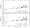 |
Fig. 4 Differential abundances (ζ2 Ret – ζ1 Ret) against condensation temperature. The abundances are derived for the combined spectra and spectra that were used in S16. The black dashed line and red line are the same as in Fig. 3. |
Since the differential abundances of the stars relative to the Sun can be affected by several factors, such as GCE, age, or the relative effect of NLTE on stars with similar, but not exactly the same stellar parameters, and we are interested in testing whether the two stars of the binary system show different refractory-to-volatile element ratios, in Fig. 4 we plot the differential abundances of ζ1 Ret relative to ζ2 Ret. The plot and corresponding Table 2 shows that there is a strong and significant correlation with the Tc in both cases when all of the elements and only refractory elements are considered for the linear regression. The slopes derived from the combined and S16 spectra are very similar, but the errors of the slopes for the case of combined spectra are smaller and the significance is higher. Following the interpretation of Meléndez et al. (2009), in S16 the authors based on this result proposed that refractory elements depleted in ζ2 Ret are locked up in the debris disk that the star hosts.
To test the hypothesis that the observed Tc trend is due to the presence of a debris around ζ2 Ret, we performed the following test. We used the three highest S/N individual spectra for each star (ζ1 Ret and ζ2 Ret) and derived differential abundances for each star using different spectra as reference. The results are plotted in Fig. 5 and presented in Table 2. This test clearly shows that the slope of the Tc trend significantly changes depending on which pair of spectra are compared. It is interesting to note that some of the observed trends are relatively significant (e.g., ζ2 Ret_b – ζ2 Ret_a). These results, in turn, mean that if different spectra of the two stars are used to derive the Tc trend between the two stars, very different results can be obtained, ranging in significance from nonsignificant (i.e., having a slope compatible with zero) to very significant.
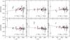 |
Fig. 5 Differential abundances against condensation temperature for ζ1 Ret and ζ2 Ret, derived from three highest S/N individual spectra. The black dashed line and red line are the same as in Fig. 3. |
It is difficult to identify the main reason(s) of the observed Tc trend between different spectra of the same star. All of the spectra are observed with the same, and most stable spectrograph, HARPS, which minimizes the possible effects of spectral resolution and instrumental profile. While the three spectra of ζ2 Ret are taken at different dates (on 11 August 2006, 27 August 2009, and 31 January 2010, for ζ2 Ret_a, ζ2 Ret_b, and ζ2 Ret_c, respectively), the selected three individual high S/N spectra of ζ1 Ret are taken on the same night (15 November 2005). This means that time-dependent systematics are much less likely to play an important role for the observed trend for ζ1 Ret. This could be the reason that the Tc slopes for this star are less significant compared to those of its companion. The two stars exhibit different levels of activity; ζ1 Ret ( ) is more active than ζ2 Ret (
 ) (Zechmeister et al. 2013). Although ζ1 Ret is more active than its companion, the stellar variability should not play a significant role in the observed difference in the chemical abundances between the different spectra of the star since, again, the observations are carried out on the same night.
Recently, Bedell et al. (2014) analyzed solar spectra observed with different instruments, from different asteroids, and at different times, i.e, conditions. The authors reached a conclusion that the major effect on differential relative abundances is caused by the use of different instruments. They also found no significant (more than 2σ) Tc trend between the different spectra they used.
One of the main factors that can produce (or affect) the Tc trend is the correct derivation of stellar parameters and their errors. Different elements (and corresponding spectral lines) show different sensitivities to atmospheric temperature (depending on the excitation potential), surface gravity (depending on the ionization state), and stellar metallicity (see, e.g., Adibekyan et al. 2012c).
Another very important factor that can determine the Tc slope is the error estimation for the individual elements. Since we use the errors as weights for each abundance, the elements with the smallest errors have the largest weights and may determine the slope and its confidence interval. As discussed in Sect. 3, the errors can be underestimated only if two lines are used and the line-to-line dispersion is used to estimate the errors on the EWs. It is also important to mention the high weights of elements with a large number of lines in the derivation of the Tc slopes. Since the error of the abundances is calculated as a σ/, the elements such as Ni and Ti, which have many spectral lines, show the smallest errors and, hence, have a key role in the determination of the slope value.
The importance of the errors of individual chemical abundances is well illustrated in Figs. A.1−A.3, and in Table A.1. In these plots and table, we present the derivation of the Tc slopes for the above discussed stars and spectra, but applying OLS, i.e., no errors (or equal errors) are considered. We can clearly see that for the same star or spectra the OLS and WLS give very different results. Table A.1 also shows that the most significant trends are observed for (ζ1 Ret_comb – ζ2 Ret_comb), (ζ2 Ret_b – ζ2 Ret_a), and (ζ2 Ret_c – ζ2 Ret_a). Moreover, the only significant trend that remains when considering only the refractory elements with Tc> 900K is for the (ζ2 Ret_c – ζ2 Ret_a) pair.
6. Conclusion
The ζ Reticuli binary system, composed of two solar analogs, is a very interesting and well-known system not only in the scientific literature, but also in science fiction literature9 and movies,10 as a word of Zeta Reticulans11.
Both stars of this binary system are in planet search programs and the presence of short-period small (or massive) planets or larger period massive planets can be excluded (see S16). However, there is indirect evidence that the ζ2 Ret may have a massive eccentric companion that perturbed its eccentric debris disk (Faramaz et al. 2014).
We used several high-quality (S/N> 360) individual and combined spectra (S/N of 1300 and 3000) of ζ1 Ret and ζ2 Ret to revisit the results obtained in S16, namely that ζ2 Ret shows a deficit of refractory elements (relative to volatiles) when compared to ζ1 Ret probably because of the presence of the debris disk that ζ2 Ret hosts. We first derived the stellar parameters using the classical (nondifferential) method, then applied careful line-by-line differential abundance analysis of the stars relative to the Sun and relative to each other.
When we consider the combined, highest S/N spectra of the two stars we obtain similar Tc trend as was reported in S16. The trend exists when all of the elements and only refractory elements are considered in the derivation of the Tc slope. We also show that when comparing the chemical abundances of the same individual stars (ζ1 Ret with ζ1 Ret and ζ2 Ret with ζ2 Ret) derived from different individual spectra, we observe different and sometimes significant Tc trends. The trends observed between different individual spectra of ζ1 Ret that are observed during the same night, are less significant than those observed for the ζ2 Ret that are observed on different nights.
In this context, there is no consensus on the results of the Tc trend for some individual systems (e.g., 16 Cyg AB; Laws & Gonzalez 2001; Takeda 2005; Schuler et al. 2011a; Tucci Maia et al. 2014). The reported differences can be due to the same sort of effect that we discussed in this study.
Our results show that when studying tiny chemical abundance trends with condensation temperature, it is very important to use very high-quality combined spectra. The combination of several spectra increase the S/N and may minimize possible time-dependent effects. The results also show that there are other nonastrophysical factors (such as over- or underestimation of the errors of the individual elements) that may be responsible for the observed Tc trends and indicate that one should be very careful when analyzing very subtle differences in chemical abundances between stars. However, we should stress that this result does not imply that all of the observed Tc trends do not have an astrophysical origin.
We note that Ramírez et al. (2014) also observed a correlation between the Tc slope and stellar age for metal-rich solar analogs, but apparently with opposite sign. In contrast to our results, they found that most refractory element depleted stars are younger than the those with the highest refractory element abundances.
The last version of ARES code (ARES v2) can be downloaded at http://www.astro.up.pt/~sousasag/ares
The source code of MOOG can be downloaded at http://www.as.utexas.edu/~chris/moog.html
Acknowledgments
This work was supported by Fundação para a Ciência e Tecnologia (FCT) through national funds (project ref. PTDC/FIS-AST/7073/2014) and by FEDER through COMPETE2020 (project ref. POCI-01-0145-FEDER-007672). This work was also supported by FCT through the research grants (ref. PTDC/FIS-AST/7073/2014 and ref. PTDC/FIS-AST/1526/2014) through national funds and by FEDER through COMPETE2020 (ref. POCI-01-0145-FEDER-016880 and ref. POCI-01-0145-FEDER-016886). This work results within the collaboration of the COST Action TD1308. P.F., N.C.S., and S.G.S. also acknowledge the support from FCT through Investigador FCT contracts of reference IF/01037/2013, IF/00169/2012, and IF/00028/2014, respectively, and POPH/FSE (EC) by FEDER funding through the program “Programa Operacional de Factores de Competitividade − COMPETE”. P.F. further acknowledges support from FCT in the form of an exploratory project of reference IF/01037/2013CP1191/CT0001. V.A. and E.D.M acknowledge the support from the FCT in the form of the grants SFRH/BPD/70574/2010 and SFRH/BPD/76606/2011, respectively. V.A. also acknowledges the support from COST Action TD1308 through STSM grant with reference Number: COST-STSM-TD1308-32051. G.I. acknowledges financial support from the Spanish Ministry project MINECO AYA2011-29060. JIGH acknowledges financial support from the Spanish Ministry of Economy and Competitiveness (MINECO) under the 2013 Ramón y Cajal program MINECO RYC-2013-14875, and the Spanish ministry project MINECO AYA2014-56359-P.
References
- Adibekyan, V. Z., Delgado Mena, E., Sousa, S. G., et al. 2012a, A&A, 547, A36 [NASA ADS] [CrossRef] [EDP Sciences] [Google Scholar]
- Adibekyan, V. Z., Santos, N. C., Sousa, S. G., et al. 2012b, A&A, 543, A89 [NASA ADS] [CrossRef] [EDP Sciences] [Google Scholar]
- Adibekyan, V. Z., Sousa, S. G., Santos, N. C., et al. 2012c, A&A, 545, A32 [NASA ADS] [CrossRef] [EDP Sciences] [Google Scholar]
- Adibekyan, V. Z., González Hernández, J. I., Delgado Mena, E., et al. 2014, A&A, 564, L15 [NASA ADS] [CrossRef] [EDP Sciences] [Google Scholar]
- Adibekyan, V., Figueira, P., & Santos, N. C. 2015a, ArXiv e-prints [arXiv:1509.02429] [Google Scholar]
- Adibekyan, V., Figueira, P., Santos, N. C., et al. 2015b, A&A, 583, A94 [NASA ADS] [CrossRef] [EDP Sciences] [Google Scholar]
- Adibekyan, V., Santos, N. C., Figueira, P., et al. 2015c, A&A, 581, L2 [NASA ADS] [CrossRef] [EDP Sciences] [Google Scholar]
- Asplund, M., Grevesse, N., Sauval, A. J., & Scott, P. 2009, ARA&A, 47, 481 [NASA ADS] [CrossRef] [Google Scholar]
- Bedell, M., Meléndez, J., Bean, J. L., et al. 2014, ApJ, 795, 23 [NASA ADS] [CrossRef] [Google Scholar]
- Bertran de Lis, S., Delgado Mena, E., Adibekyan, V. Z., Santos, N. C., & Sousa, S. G. 2015, A&A, 576, A89 [NASA ADS] [CrossRef] [EDP Sciences] [Google Scholar]
- Biazzo, K., Gratton, R., Desidera, S., et al. 2015, A&A, 583, A135 [NASA ADS] [CrossRef] [EDP Sciences] [Google Scholar]
- Bond, J. C., O’Brien, D. P., & Lauretta, D. S. 2010, ApJ, 715, 1050 [NASA ADS] [CrossRef] [Google Scholar]
- Cayrel, R. 1988, in The Impact of Very High S/N Spectroscopy on Stellar Physics, eds. G. Cayrel de Strobel, & M. Spite, IAU Symp., 132, 345 [Google Scholar]
- Delgado Mena, E., Israelian, G., González Hernández, J. I., et al. 2010, ApJ, 725, 2349 [NASA ADS] [CrossRef] [Google Scholar]
- Delgado Mena, E., Israelian, G., González Hernández, J. I., et al. 2014, A&A, 562, A92 [NASA ADS] [CrossRef] [EDP Sciences] [Google Scholar]
- Delgado Mena, E., Bertrán de Lis, S., Adibekyan, V. Z., et al. 2015, A&A, 576, A69 [NASA ADS] [CrossRef] [EDP Sciences] [Google Scholar]
- Dorn, C., Khan, A., Heng, K., et al. 2015, A&A, 577, A83 [EDP Sciences] [Google Scholar]
- Ecuvillon, A., Israelian, G., Santos, N. C., Mayor, M., & Gilli, G. 2006, A&A, 449, 809 [NASA ADS] [CrossRef] [EDP Sciences] [Google Scholar]
- Faramaz, V., Beust, H., Thébault, P., et al. 2014, A&A, 563, A72 [NASA ADS] [CrossRef] [EDP Sciences] [Google Scholar]
- Figueira, P., Faria, J. P., Adibekyan, V. Z., Oshagh, M., & Santos, N. C. 2016, ArXiv e-prints [arXiv:1601.05107] [Google Scholar]
- Gaidos, E. 2015, ApJ, 804, 40 [NASA ADS] [CrossRef] [Google Scholar]
- Gilli, G., Israelian, G., Ecuvillon, A., Santos, N. C., & Mayor, M. 2006, A&A, 449, 723 [NASA ADS] [CrossRef] [EDP Sciences] [Google Scholar]
- Gonzalez, G. 1997, MNRAS, 285, 403 [NASA ADS] [CrossRef] [Google Scholar]
- González Hernández, J. I., Israelian, G., Santos, N. C., et al. 2010, ApJ, 720, 1592 [NASA ADS] [CrossRef] [Google Scholar]
- González Hernández, J. I., Delgado-Mena, E., Sousa, S. G., et al. 2013, A&A, 552, A6 [NASA ADS] [CrossRef] [EDP Sciences] [Google Scholar]
- Kang, W., Lee, S.-G., & Kim, K.-M. 2011, ApJ, 736, 87 [NASA ADS] [CrossRef] [Google Scholar]
- Kurucz, R. L. 1993, SYNTHE spectrum synthesis programs and line data, Kurucz CD-ROM (Cambridge, MA: Smithsonian Astrophysical Observatory) [Google Scholar]
- Laws, C., & Gonzalez, G. 2001, ApJ, 553, 405 [NASA ADS] [CrossRef] [Google Scholar]
- Liu, F., Asplund, M., Ramírez, I., Yong, D., & Meléndez, J. 2014, MNRAS, 442, L51 [NASA ADS] [CrossRef] [Google Scholar]
- Lodders, K. 2003, ApJ, 591, 1220 [NASA ADS] [CrossRef] [Google Scholar]
- Mack, III, C. E., Stassun, K. G., Schuler, S. C., Hebb, L., & Pepper, J. A. 2016, ApJ, 818, 54 [NASA ADS] [CrossRef] [Google Scholar]
- Maldonado, J., & Villaver, E. 2016, A&A, 588, A98 [NASA ADS] [CrossRef] [EDP Sciences] [Google Scholar]
- Maldonado, J., Eiroa, C., Villaver, E., Montesinos, B., & Mora, A. 2015, A&A, 579, A20 [NASA ADS] [CrossRef] [EDP Sciences] [Google Scholar]
- Mayor, M., Pepe, F., Queloz, D., et al. 2003, The Messenger, 114, 20 [NASA ADS] [Google Scholar]
- Meléndez, J., Asplund, M., Gustafsson, B., & Yong, D. 2009, ApJ, 704, L66 [NASA ADS] [CrossRef] [Google Scholar]
- Morey, R. D., Hoekstra, R., Rouder, J. N., Lee, M. D., & Wagenmakers, E.-J. 2015, Psychonomic Bull. Rev., 23, 103 [CrossRef] [Google Scholar]
- Neuforge-Verheecke, C., & Magain, P. 1997, A&A, 328, 261 [NASA ADS] [Google Scholar]
- Nissen, P. E. 2015, A&A, 579, A52 [NASA ADS] [CrossRef] [EDP Sciences] [Google Scholar]
- Önehag, A., Gustafsson, B., & Korn, A. 2014, A&A, 562, A102 [NASA ADS] [CrossRef] [EDP Sciences] [Google Scholar]
- Patil, A., Huard, D., & Fonnesbeck, C. J. 2010, J. Stat. Software, 35, 1 [Google Scholar]
- Prochaska, J. X., Naumov, S. O., Carney, B. W., McWilliam, A., & Wolfe, A. M. 2000, AJ, 120, 2513 [NASA ADS] [CrossRef] [Google Scholar]
- Ramírez, I., Meléndez, J., & Asplund, M. 2009, A&A, 508, L17 [NASA ADS] [CrossRef] [EDP Sciences] [Google Scholar]
- Ramírez, I., Meléndez, J., & Asplund, M. 2014, A&A, 561, A7 [NASA ADS] [CrossRef] [EDP Sciences] [Google Scholar]
- Ramírez, I., Khanal, S., Aleo, P., et al. 2015, ApJ, 808, 13 [NASA ADS] [CrossRef] [Google Scholar]
- Reddy, B. E., Tomkin, J., Lambert, D. L., & Allen de Prieto, C. 2003, MNRAS, 340, 304 [NASA ADS] [CrossRef] [Google Scholar]
- Robinson, S. E., Laughlin, G., Bodenheimer, P., & Fischer, D. 2006, ApJ, 643, 484 [NASA ADS] [CrossRef] [Google Scholar]
- Saffe, C., Flores, M., & Buccino, A. 2015, A&A, 582, A17 [NASA ADS] [CrossRef] [EDP Sciences] [Google Scholar]
- Saffe, C., Flores, M., Jaque Arancibia, M., Buccino, A., & Jofre, E. 2016, A&A, 588, A81 [NASA ADS] [CrossRef] [EDP Sciences] [Google Scholar]
- Santos, N. C., Adibekyan, V., Mordasini, C., et al. 2015, A&A, 580, L13 [NASA ADS] [CrossRef] [EDP Sciences] [Google Scholar]
- Schuler, S. C., Cunha, K., Smith, V. V., et al. 2011a, ApJ, 737, L32 [NASA ADS] [CrossRef] [Google Scholar]
- Schuler, S. C., Flateau, D., Cunha, K., et al. 2011b, ApJ, 732, 55 [NASA ADS] [CrossRef] [Google Scholar]
- Smith, V. V., Cunha, K., & Lazzaro, D. 2001, AJ, 121, 3207 [NASA ADS] [CrossRef] [Google Scholar]
- Sneden, C. A. 1973, Ph.D. Thesis, The University of Texas at Austin [Google Scholar]
- Sousa, S. G. 2014, ArXiv e-prints [arXiv:1407.5817] [Google Scholar]
- Sousa, S. G., Santos, N. C., Adibekyan, V., Delgado-Mena, E., & Israelian, G. 2015, A&A, 577, A67 [NASA ADS] [CrossRef] [EDP Sciences] [Google Scholar]
- Sozzetti, A., Yong, D., Carney, B. W., et al. 2006, AJ, 131, 2274 [NASA ADS] [CrossRef] [Google Scholar]
- Takeda, Y. 2005, PASJ, 57, 83 [NASA ADS] [Google Scholar]
- Takeda, Y., Sato, B., Kambe, E., et al. 2001, PASJ, 53, 1211 [NASA ADS] [CrossRef] [Google Scholar]
- Teske, J. K., Ghezzi, L., Cunha, K., et al. 2015, ApJ, 801, L10 [NASA ADS] [CrossRef] [Google Scholar]
- Teske, J. K., Khanal, S., & Ramírez, I. 2016, ApJ, 819, 19 [NASA ADS] [CrossRef] [Google Scholar]
- Thiabaud, A., Marboeuf, U., Alibert, Y., et al. 2014, A&A, 562, A27 [NASA ADS] [CrossRef] [EDP Sciences] [Google Scholar]
- Tucci Maia, M., Meléndez, J., & Ramírez, I. 2014, ApJ, 790, L25 [NASA ADS] [CrossRef] [Google Scholar]
- Zechmeister, M., Kürster, M., Endl, M., et al. 2013, A&A, 552, A78 [NASA ADS] [CrossRef] [EDP Sciences] [Google Scholar]
Appendix A: Tc slope in OLS
In this section we present the calculation of the Tc slopes for the stars without considering the errors of the individual chemical abundances.
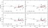 |
Fig. A.1 Same as Fig. 3, but the slopes are calculated without considering the errors of the individual abundances. |
Slopes of the [X/H] vs. Tc for different pairs of spectra.
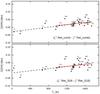 |
Fig. A.2 Same as Fig. 4, but the slopes are calculated without considering the errors of the individual abundances. |
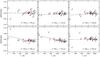 |
Fig. A.3 Same as Fig. 5, but the slopes are calculated without considering the errors of the individual abundances. |
All Tables
Stellar parameters, S/N, and observation dates of ζ1 Ret and ζ2 Ret derived from individual and combined spectra.
All Figures
|
Fig. 1 Iron abundance vs. excitation potential (upper panels) and iron abundance vs. reduced EW (lower panels) for ζ1 Ret_comb and ζ2 Ret_comb. The blue and red symbols correspond to the neutral and ionized iron lines. The black solid line indicates the linear fit of the data. |
| In the text | |
|
Fig. 2 Spectral regions containing oxygen lines in ζ1 Ret_comb, ζ2 Ret_comb, ζ1 Ret_S16, and ζ2 Ret_S16 spectra. |
| In the text | |
|
Fig. 3 Differential abundances [X/H] against condensation temperature for ζ1 Ret and ζ2 Ret. The abundances are derived relative to the Sun with the combined spectra and spectra from S16. The black dashed line represents the trend when all of the elements are used for the linear regression and the red line is the result of the linear regression when only elements with Tc> 900 K are used. |
| In the text | |
|
Fig. 4 Differential abundances (ζ2 Ret – ζ1 Ret) against condensation temperature. The abundances are derived for the combined spectra and spectra that were used in S16. The black dashed line and red line are the same as in Fig. 3. |
| In the text | |
|
Fig. 5 Differential abundances against condensation temperature for ζ1 Ret and ζ2 Ret, derived from three highest S/N individual spectra. The black dashed line and red line are the same as in Fig. 3. |
| In the text | |
|
Fig. A.1 Same as Fig. 3, but the slopes are calculated without considering the errors of the individual abundances. |
| In the text | |
|
Fig. A.2 Same as Fig. 4, but the slopes are calculated without considering the errors of the individual abundances. |
| In the text | |
|
Fig. A.3 Same as Fig. 5, but the slopes are calculated without considering the errors of the individual abundances. |
| In the text | |
Current usage metrics show cumulative count of Article Views (full-text article views including HTML views, PDF and ePub downloads, according to the available data) and Abstracts Views on Vision4Press platform.
Data correspond to usage on the plateform after 2015. The current usage metrics is available 48-96 hours after online publication and is updated daily on week days.
Initial download of the metrics may take a while.