| Issue |
A&A
Volume 591, July 2016
|
|
|---|---|---|
| Article Number | A91 | |
| Number of page(s) | 11 | |
| Section | Interstellar and circumstellar matter | |
| DOI | https://doi.org/10.1051/0004-6361/201527703 | |
| Published online | 21 June 2016 | |
Closer view of the IGR J11014-6103 outflows
1
Université de Genève, Departement d’Astronomie –
ISDC, chemin d’Écogia
16, 1290
Versoix,
Switzerland
e-mail:
This email address is being protected from spambots. You need JavaScript enabled to view it.
2
Institut für Astronomie und Astrophysik, Universität
Tübingen, Sand 1,
72076
Tübingen,
Germany
3
Max-Planck-Institut für Kernphysik Saupfercheckweg
1, 69117
Heidelberg,
Germany
4
Western Sydney University, Locked Bag 1797, Penrith South DC, NSW
1797,
Australia
5
Department for Astrophysics, University of Vienna,
Türkenschanzstr. 17,
1180
Vienna,
Austria
Received: 5 November 2015
Accepted: 5 April 2016
Abstract
IGR J11014-6103 (also known as the Lighthouse Nebula) is composed of a bow-shock pulsar wind nebula (PWN) and large-scale X-ray jet-like features, all powered by PSR J1101-6101. Previous observations suggest that the jet features stem from a ballistic jet of relativistic particles. In order to confirm the nature of the jet and the counter-jet, we obtained a new deep 250 ks Chandra observation of the Lighthouse Nebula. We performed detailed spatial and spectral analysis of all X-ray components of the system. The X-ray PWN is now better resolved and shows a peculiar morphology resembling the shape of an arrow. The overall helical pattern of the main jet is confirmed. However, there are large deviations from a simple helical model at small and large scales. Significant extended emission is now detected, encompassing the main jet all along its length. The presence of an apparent gap along the main jet at ~50″ distance from the pulsar is confirmed; however, the surrounding extended emission prevents conclusions on the coherence at this position of the jet. The counter-jet is now detected at high statistical significance. In addition, we found two small-scale arcs departing from the pulsar towards the jets. We also looked for possible bow-shock emission due to the pulsar motion, with a short VLT/FORS2 H-α observation. No clear emission is found, most likely because of the contamination from a diffuse nebulosity. The results of our X-ray analysis show that both a ballistic jet scenario and an alternative scenario involving the diffusion of particles along pre-existing interstellar magnetic field lines are able to satisfactorily explain some of the observational evidence, but cannot fully reproduce the observations.
Key words: X-rays: individuals: IGR J11014-6103 / stars: neutron / stars: jets / ISM: jets and outflows / ISM: supernova remnants / supernovae: individual: MSH 11-61A
© ESO, 2016
1. Introduction
Neutron stars are one of the possible end points of the stellar evolution and are produced in most cases through the degenerate collapse of the core of a massive star (once the internal part of the star has reached an unstable condition). This core-collapse supernova explosion can provide a strong natal kick to the newly born neutron star, which can consequently move with high velocity into the ambient medium (see e.g. the review by Janka 2012). Detailed analyses of the galactic pulsar population found a mean velocity of vPSR ~ 400 km s-1 (Hobbs et al. 2005). The highest velocity directly measured is that of PSR B1508+55 with  km s-1 (Chatterjee et al. 2005).
When the spatial velocity of a pulsar is sufficiently large, it will escape its progenitor’s supernova remnant (SNR) while the remnant is still young and actively emitting in X-rays. The subsequent pulsar’s motion in the interstellar medium (ISM) is typically supersonic. In this case, a bow-shock is generated and the swept-up matter prevents the wind expelled by the pulsar from propagating in the direction of motion. This wind is collimated backwards, forming a nebula confined in a conical shape whose aperture angle depends, among other parameters, on the pulsar linear velocity (for a review see e.g. Gaensler 2005).
MSH 11-61A (also known as G290.1-0.8) is a mixed morphology SNR detected from radio to soft X-rays (up to ~3 keV) that was formed by the core collapse of a massive progenitor star (mass ≳25 M⊙; Filipović et al. 2005; Reynoso et al. 2006; García et al. 2012; Kamitsukasa et al. 2015; Auchettl et al. 2015a). Following these authors, the distance to the SNR is in the range 6−11 kpc; the most recently determined values converge towards 7 ± 1 kpc. We adopt a distance of 7 kpc throughout the paper1. The INTEGRAL source IGR J11014-6103 is located close to MSH 11-61A and is powered by PSR J1101-6101 (Pavan et al. 2011, hereafter Paper I; Tomsick et al. 2012; Pavan et al. 2014, hereafter Paper II; Halpern et al. 2014). The pulsar shows spin-down parameters typical for pulsars of its age: a period of P = 62.8 ms and a pulse period derivative Ṗ = (8.56 ± 0.51) × 10-15 s s-1. The estimated spin-down energy is Ė = 1.36 × 1036 erg s-1 and the surface dipolar magnetic field is 7.4 × 10¹¹ G (Halpern et al. 2014). Previous Chandra observations aimed at the INTEGRAL source showed that PSR J1101-6101 simultaneously powers several outflows: an X-ray and radio PWN, shaped in a narrow cone elongated towards the parent SNR, and an X-ray jet and counter-jet, both oriented nearly perpendicular to the PWN axis (Tomsick et al. 2012; Paper II). The main jet extends for nearly 5′ in the sky, which corresponds to a projected length of ~11 pc, and showed a remarkable helicoidal pattern (see Paper II). Already in the data set analysed in Paper II, indications for a spatial deviation from the helical pattern of the main jet were noticed at a distance of ~50″ from the pulsar. At this position the surface brightness of the jet was low, forming what looked like a gap, but its brightness profile was compatible with expectations of Doppler-deboosting in the jet-helix model. The spatial deviation was therefore not considered significant at the time because the data were hampered by the presence of CCD chip gaps, resulting in only 50% effective exposure in that region. The counter-jet was detected at 3.7σ in the Chandra image and its flux was estimated to be ~5% that of the main jet. The conical shape of the PWN in IGR J11014-6103 was ascribed to the supersonic motion of PSR J1101-6101 in the ISM (Tomsick et al. 2012).
Although several examples of bow-shock pulsar wind nebulae (bsPWNe) have now been detected in connection with their pulsars travelling at supersonic velocities in the interstellar medium (see e.g. Gaensler et al. 2004; McGowan et al. 2006; Kargaltsev & Pavlov 2008), only a few other systems share a geometry similar to the one seen in the Lighthouse Nebula: the Guitar Nebula, powered by PSR B2224+65 (Cordes et al. 1993; Chatterjee & Cordes 2002; Johnson & Wang 2010; Hui et al. 2012), and possibly the PWN system powered by PSR J1509-5850, for which the presence of a large-scale outflow misaligned to the direction of motion have only very recently been reported (Klingler et al. 2016). Similarly to the IGR J11014-6103 case, the Guitar Nebula’s pulsar is producing a bright and elongated X-ray jet, extending over ~1 pc in a direction almost perpendicular to the pulsar direction of motion. In both the Lighthouse Nebula and the Guitar Nebula, the mechanism leading to the production of such peculiar jets is still poorly understood (Bandiera 2008; Johnson & Wang 2010; Paper I; Hui et al. 2012; Paper II).
To solve a series of questions that could not be conclusively addressed with the previous data set, in 2014 we obtained a much deeper Chandra X-ray observation (250 ks) of IGR J11014-6103. We describe the analysis of these data in Sect. 2. We also report on the analysis of an exploratory observation performed with VLT to search for possible H-α emission close to PSR J1101-6101 (Sect. 3). In Sect. 4 we discuss the results of our data analyses and provide our conclusion in Sect. 5.
2. Chandra X-ray observations and data analysis
While our initial Chandra observation was aimed at imaging the pulsar and the PWN (Paper II) with the highest accuracy, we aimed the new observation in order to investigate the complex morphology of the main jet. The observation was split into five smaller exposures because of planning constraints (see Table 1). We then chose to optimise the pointing displacement to have the main jet and the pulsar entirely included in a single CCD in order to optimally investigate the gap region along the main jet, and the region connecting the pulsar and the jet base. This was achieved with a simZ offset of 6.0 mm and a Y offset of 1.0′. The offsets were kept identical in all exposures to ensure a good handling of the combined events. The data were processed with Chandra CIAO v.4.7, using the latest available calibrations (CALDB v. 4.6.7). All observations were reprocessed with the CIAO tool chandra_repro, using vfaint mode background cleaning and subpixel resolution (edser method), unless differently specified. After cleaning, we verified that the vfaint filter used did not significantly affect the event counts of the extended structures in IGR J11014-6103. Only the pulsar was partially affected by this filter, with ~6% of good events being rejected. Therefore, we used the vfaint background cleaned evt2 files for the following analysis. We also verified that the observations were not affected by high flaring background. The effective final exposure time was 247 ks.
By computing and inspecting the point spread function (PSF) map of each observation, we verified that in all cases the characteristics of the instrument PSF were constant in the region including the pulsar, the jets, and the PWN.
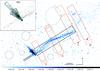 |
Fig. 1 Chandra 250 ks mosaic of the Lighthouse Nebula (exposure corrected and smoothed with a Gaussian kernel of σ = 1.5 pixel). The colour scale at the bottom of the plot is in units of photon/cm2/s. Solid red rectangles a–d (and the corresponding dashed background boxes) indicate the regions used to extract brightness profiles perpendicularly to the main jet (Sect. 2.3). The regions used for spectral extraction are also shown: the average spectra of the main jet, the counter-jet, and the PWN were extracted from the solid black regions (Sect. 2.4.1). For the point source PSR J1101-6101 we used a circle of radius 1.6′′ centred on the pulsar position (not shown). Background regions are marked with dashed black circles. In the inset: the details of the PWN shape and the attaching points of the two jets to the pulsar are visible. Coloured rectangles along the PWN indicate the regions used to extract spatially resolved spectra (Sect. 2.4.2). In this image, as in the rest of the paper, north is up and east is to the left. |
Summary of the Chandra observations of IGR J11014-6103.
2.1. Imaging
The new observations were combined in an exposure corrected mosaic with the ciao tool merge_obs, in the energy range 0.5−7 keV (see Fig. 1). The main spatial features seen in this mosaic are as listed here:
PWN: the PWN has a sharp conical shape, but it also shows a more extended and collimated component. The overall structure resembles the shape of an arrow, with the “shaft” extending over ~1.7′ in a compact cylindrical shape, and the “head” spanning a wider and slightly dimmer cone, with an aperture of ~30° up to ~0.7′ from the pulsar (see inset in Fig. 1). Comparing the new image to our previous 50 ks observation, we note that the same structure was also present in that case, although less evident because of the lower statistics.
Counter-jet: the counter-jet is now detected with a high significance and it extends remarkably linearly for 1.5′ to the SE. It appears to be somewhat aligned with the first 50′′ of the main jet, and is thus not pointing directly at the pulsar position. Within ~18′′ from the pulsar, the linear counter-jet stops abruptly and the mosaic reveals instead an arched structure (described below), pointing towards the pulsar.
Main jet: the main jet still shows the same overall pattern found in our previous shorter observation (Paper II), including a gap at about 50−90′′ from the pulsar. In the previous observation this region was coincident with a factor two lower exposure due to the presence of ACIS chip gaps; instead, the new data have equal exposure along the jet without chip gaps or other significant dead chip columns. We can thus confirm that the gap feature is intrinsic to the emission from this region, and not due to instrumental artefacts. Lower surface-brightness emission is now also clearly detected, enshrouding the jet all along its length. Because of this emission, it is not possible to determine whether the gap is a true spatial break/decollimation of the jet or whether the emission from the main jet is just dimming and overlapping with the surrounding emission in this region (see also Sect. 2.3).
Arcs: in addition to the main spatial features described above, visual inspection of the mosaic image at small scales around the pulsar reveals the presence of an arc departing from the pulsar and oriented towards the counter-jet (see inset in Fig. 1). We also detected hints of a second almost symmetric arc placed on the west side of the pulsar and directed towards the main jet. The arcs are visible up to ~12′′ and 18′′ from the pulsar, respectively. Because of the relatively low signal-to-noise ratio (S/N) level of the arc emission at larger distances from the pulsar and the presence of diffuse emission around the edge of the PWN, it is impossible to verify whether this arc structure (and possibly also the symmetric one) exists only between the pulsar and the base of the counter-jet, or if it extends further.
To reveal the signal in low surface-brightness regions, we extracted an adaptively binned image of the Lighthouse Nebula by applying the Voronoi tessellation algorithm (Cappellari & Copin 2003), as implemented in Eckert et al. (2015). We used a target S/N of 3 for the algorithm, which allows us to visualise statistically significant brightness variations across the nebula. The resulting image is shown in Fig. 2. All the known structures of the Lighthouse Nebula (pulsar, PWN, main jet and counter-jet) are detected at high significances, as is the diffuse emission around the main jet. This diffuse emission appears organised in “stripes” that are almost parallel to the main jet and more prominent at its far end. Closer to the pulsar, the algorithm is not able to resolve the apparent parallel lines (Fig. 1), and the emission appears more diffused. This broad region of emission encircling the main jet is analysed in more detail in Sects. 2.3 and 2.5.
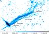 |
Fig. 2 Mosaic image of IGR J11014-6103 with Voronoi adaptive binning. Each cell in this image has a S/N ≥ 3. The image is colour-coded in units of photon/cm2/s/arcmin2 as detailed in the colour map at the bottom of the plot. The pulsar, the main jet, the counter-jet, and the PWN are all detected at high significance. The broader emission around the main jet is also clearly detected. The black ruler shows linear distances along the jet. |
2.2. Pulsar proper motion
The absolute astrometric accuracy of 0.6′′ of Chandra permits sensitive proper motion searches of bright point-like sources and in particular of isolated pulsars by comparing the position measured in observations separated by several years (see e.g. Auchettl et al. 2015b; Van Etten et al. 2012; Motch et al. 2009). Moreover, the relative positional accuracy between different observations can be significantly improved with respect to the absolute accuracy by removing systematic uncertainties that affect the different observations in the same way2. Here, we used our previous 50 ks observation and the new 250 ks Chandra observation of IGR J11014-6103 to search for the proper motion of the pulsar (details of each observation are listed in Table 1). In each observation, the pulsar is almost on-axis, although the telescope was operated in different configurations. To study the pulsar and the surrounding region, we used event files reprocessed without the vfaint mode background cleaning, as we included the old observation performed in FAINT mode. We used as reference frame Obs ID 16007, which has the longest exposure time (116 ks) and therefore the largest number of field point sources detected. We then registered with the CIAO tool wcs_match all other exposures by creating a list of common field point sources with a detection significance above 4σ in each frame3 to minimise the observed displacements. The number of common field sources between the reference frame (where we identified a total of 36 field sources satisfying the above criteria) and each of the other frames varied between 8 and 20, depending on the frame exposure. We corrected the reference positions for known proper motions of the field sources (we found four field point sources with optical counterpart in USNO B-2, for which a significant proper motion is known).
By comparing the residuals of the field source positions after registration of the frames, we found a relative positional accuracy of 0.2′′ between all observations. We verified that inclusion or exclusion of the four sources with high proper motion does not affect the final positional accuracy. No significant pulsar displacement was detected between the different epochs (which are approximately 2 years apart), resulting in a pulsar proper motion μPSR ≤ 0.3″/yr (at 3σ level). This upper limit is not constraining as it is consistent with the expected value of 0.03′′/yr (vPSR/ 1000 km s-1)·(7 kpc /dPSR), assuming a pulsar velocity of 1000 km s-1 (Paper II).
2.3. Brightness profiles
We extracted exposure-corrected, background-subtracted brightness profiles along the PWN and the main jet, using counts in rectangular regions. We defined 20 regions along the jet, extended for 20′′ each, and 18 regions of 5′′ in length each along the PWN (see Fig. 3). From the counts recorded in each region we computed the brightness profiles with the CIAO tool dmextract. In Fig. 3, we compare the profiles extracted from the new 250 ks data with those obtained from the same regions in the previous 50 ks observation. The images are normalised for the corresponding exposure maps, thus correcting for the effects related to the different integration time and satellite roll angle (and hence also the different positions of the chips gaps on the images). The brightness profiles, both for the PWN and main jet, do not show any relevant difference between the two observations (to within the uncertainties).
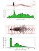 |
Fig. 3 Top panels: brightness profile as a function of distance from the pulsar, extracted along the jets, from the regions shown in the image above (the brightness in the pulsar bin is not to scale). The horizontal scale is the same in the profile plot and in the extraction region image. The black profile is computed from the new 250 ks data; for comparison the profile obtained from the previous 50 ks observation is represented with a filled green histogram. Bottom panels: same as above, but for the extraction regions along the PWN. |
Along the main jet, at 50–90′′ from the pulsar – where the images seem to show a gap – we do not measure any significant brightness decrease. In our deep mosaic (Fig. 1), a diffused emission component is also visible around the main jet. The Voronoi-binned image (Fig. 2) suggests that this emission comprises several stripes developing almost parallel to the main jet. To further investigate the structure of the region around the main jet, we computed the brightness profiles in different cuts perpendicularly to the jet (Fig. 4). These profiles clearly show multiple brightness peaks located on both sides of the main jet supporting the presence of the linear features hinted by the images. Given the relatively low S/N of the data, we are currently unable to put firm constraints on the geometrical shape of these structures; however, we discuss different possibilities of their nature in Sects. 2.5 and 4.
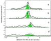 |
Fig. 4 Surface brightness profiles (black histograms) extracted in four cuts perpendicular to the main jet (see regions a–d in Fig. 1). For comparison we also plot the corresponding profiles obtained from a model with a single narrow (green histogram) or large (green solid curve) helical jet (see Sect. 2.5). In each plot the distance from the jet axis increases towards the pulsar direction of motion (SW). |
2.4. Spectra
We extracted from each Chandra observation in Table 1 all the spectra that are described in Sects. 2.4.1 and 2.4.2 with the CIAO tool specextract, computing at the same time the ancillary response file (ARF) and the response matrix file (RMF) of each data set. We used the same extraction regions in all frames, and then combined the spectra of the same region with the CIAO tool combine_spectra. This allowed us to obtain merged spectra with higher S/N and their corresponding weighted ARF and RMF. We verified that compatible results within the statistical uncertainties were provided by using the combined spectra or by fitting the spectra from the various Obs ID simultaneously. In the following we thus discuss only the combined spectra.
2.4.1. Average spectra of the extended regions
We extracted the average spectra of the pulsar, the PWN, and the jets from the regions defined in Fig. 1. The extraction regions were chosen to avoid the chip gaps in each exposure wherever possible. The only exception to this is for the counter-jet and the PWN, which fall between two chips in all Obs IDs.
All spectra are described well by a simple absorbed power-law model (reduced χ2 = 0.85–0.99). The absorption column density is estimated, here and in the following, by using a phabs model with standard XSPEC solar abundances (Anders & Grevesse 1989) and photoionisation cross sections (Balucinska-Church & McCammon 1992, 1998). The results of the spectral analysis obtained from the fits to the pulsar, the PWN, and the main jet are compatible with those reported previously in Paper II. The best fit value of Γ obtained from the main jet is significantly different from the value obtained from the PWN, as can be seen in Fig. 5. The new data on IGR J11014-6103 allowed us to extract for the first time the spectrum of the counter-jet (from the corresponding boxed region in Fig. 1). This is reliably fitted (reduced χ2 = 0.9) with a simple absorbed power-law model as well. The total flux extracted from the counter-jet is 2−3% of the total extracted main jet flux in the 2−10 keV band. The best fit parameters are reported in Table 2.
Best fit parameters for the spectra of the different Lighthouse Nebula components.
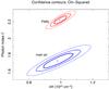 |
Fig. 5 Contour plots of the power-law fit parameters Γ and NH computed for the main jet (in blue) and the PWN (in red). Contours at 68%, 90%, and 99% confidence levels are shown for both cases. |
2.4.2. Spatially resolved spectra
In order to analyse possible spectral variations as a function of distance from the pulsar, we extracted a number of spectra from small rectangular regions covering the PWN (as shown in Fig. 1). The regions match the brightest parts of the PWN to maximise the S/N ratio. Here we used the background regions shown in Fig. 1 (the same used for the average spectra) and we verified that a different reasonable choice of the background regions did not significantly affect the results. All spectra could be accurately fit with a simple absorbed power-law model. The absorption column density remained constant within the uncertainties, and thus we fixed it at the average value of 9.9 × 1021 cm-2. The photon index distribution is shown in Fig. 6. The photon index of the PWN X-ray emission increases noticeably with the distance from the pulsar. A fit with a parabolic function gives an acceptable description of the data (reduced χ2 = 0.7) and provides a significant improvement with respect to the fit with a linear function (reduced χ2 = 2.6).
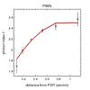 |
Fig. 6 Photon index along the PWN (uncertainties at 1σ level). The best fit with a parabolic function is shown in red. |
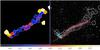 |
Fig. 7 Left panel: photon index map along the main jet and PWN. The colours represent different spectral indices, as shown in the colourbar at the bottom of the plot. Contours are drawn around the regions for clarity at levels of Γ = 1.1,1.5,1.8,2.8. Typical uncertainties on the spectral indices are of the order of ± 0.1. Right panel: the same contours are reported on the spatial map to aid the visual identification of the regions used for the spectral extractions and of the regions clustering around similar values of Γ. The region in red was used to extract spectra from the main jet. |
We performed a similar spectral analysis along the main jet. In this case, however, a more complex variation of the photon index with the distance from the pulsar is found. To study these variations in more detail, we extracted a photon index map (Fig. 7) using the method presented in Rossetti et al. (2007). We defined an adaptive 2D binning using the Voronoi tessellation technique presented in Sect. 2.1 with a target of 300 counts per bin. Then, we extracted the surface brightness in five logarithmically spaced energy bands spanning the 1−6 keV range where the main jet is predominantly emitting. We estimated the local background rate in each band and subtracted it from the data, adding in quadrature the uncertainty in the background rate. We then used XSPEC to fold the model spectrum with the Chandra response files to create a template of the expected count rate per band as a function of the photon index. The absorption column density was fixed to its mean value of NH = 9 × 1021 cm-2. A χ2 minimisation procedure was then used to fit the templates to the spectra in each individual band and estimate the photon index with its uncertainty. By analysing several background regions surrounding the main jet, we further verified that the background does not change significantly along the extended feature. The photon index map confirms the smooth spectral softening along the PWN, and the complex evolution of Γ within the main jet.
To further investigate the spectral changes along the jet, we analysed the correlation between Γ and the distance from the pulsar, and between Γ and the flux in each Voronoi bin. This analysis was repeated for the collimated main jet alone (red region in Fig. 7; right), and for the brighter emission around it. In the latter case, we did not find any significant correlation. When considering only the collimated main jet, we found that Γ follows a curved trend as a function of distance; there is a positive correlation up to ~200′′ from the pulsar, followed by a negative trend at larger distances (Fig. 8). We found no obvious trend between Γ and the flux.
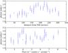 |
Fig. 8 Upper panel: photon index Γ as a function of the distance along the collimated main jet (see extraction region in red in Fig. 7). Bottom panel: same as for the upper panel, but here plotted against flux in each Voronoi cell. |
2.5. Jet model
We applied the same 2D helical model described in Paper II to the new 250 ks image to verify whether the helical pattern that we detected in the previous shorter Chandra observation can still fully account for this deeper observation. This is relevant in particular for the portion of the jet within the first 100′′ from the pulsar where the new data set confirmed the presence of a gap (see discussion in Sect. 2.3). Following the same treatment as in Paper II, we assume that counter-jet and jet are intrinsically identical and that the observed ratio between the total extracted fluxes of the two jets is due only to Doppler effects. With the refined measure of the counter-jet flux that we obtained with the current deeper observation (see Sect. 2.4.1), we inferred a mean particle bulk velocity β = 0.95. We fixed this value in our model. We used the ciao/sherpa tools in a Python environment as well as the cstat implementation of the Cash statistic4. We fit the helical model to the mosaic image, using the corresponding exposure map and adding a constant 2D function to simulate the background level. We restricted the modelling to the main jet, excluding the counter-jet and the small-scale arcs close to the pulsar.
The helical model includes a parameter used to modify the cross section of the jet around its axis (forming a 2D Gaussian cross section). Given the presence of significant diffuse emission around the main jet as discussed in Sects. 2.1, 2.3, and 2.4.2, we tuned this parameter to match the brighter collimated main jet, and in a second run we left it free to account for the diffuse emission. In both cases (i.e. when using a narrow or a broader helical model), we found fit statistics of ~1.5. This provides a significant improvement with respect to the value of 2.3 that is obtained from a flat bi-dimensional background model (i.e. with no helix). The best fit parameters that we obtained were inclination angle 38°, helical period 50 yr, and cone semi-aperture angle of 5.0° (see Paper II for the full description of the model parameters). The residual map, however, shows that the image is not reconstructed well because only the large-scale features have been reproduced. Limiting the fitting to the regions at distances greater than 90′′ from the pulsar to avoid the region of the gap along the main jet does not provide a significant improvement in the fits results. The portion of the main jet closer to the pulsar fails to be fully reproduced by the same model parameters found while fitting the regions further apart. The addition of a symmetrical helix to account for the counter-jet fails to reproduce even the main orientation of this feature (see Fig. 9). A comparison of the brightness profiles extracted from transversal cuts to the main jet (Fig. 4) shows that the single helix model does not follow well the profiles measured from the data: the narrow helical model only partly reproduces the brightness peaks of the collimated main jet, while a broad helical model fails to reproduce the profiles observed from the extended emission around the jet.
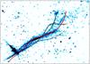 |
Fig. 9 Solid red line: best fit to the main jet with a simple helical model, superimposed on the 250 ks Chandra mosaic with Voronoi adaptive binning (Fig. 2). The model is in relatively good agreement with the shape of the jet at distances >90′′ from the pulsar; however, it fails to reproduce the regions closer to the pulsar and the counter-jet. Solid black lines represent tentative additional helices, each with a different helical phase. An additional tentative helix with different viewing angle is drawn with a dashed line. |
Motivated by these mismatches and by the presence of a significant diffuse emission distributed non-symmetrically around the main jet (see transversal cuts in Figs. 2 and 4), we tentatively included additional helical outflows in the model (see Fig. 9). Given the relatively low surface brightness of this region, we did not attempt to fit this model to the data. We inspected only qualitatively whether this phenomenological model was able to improve the description of the diffuse emission encompassing the jet with respect to the single helical model. All the parameters describing the additional helices are fixed to match those used for the main helix, except for the helical phase and normalisation. We found that the main collimated jet was better described by a helix at phase5 260 deg, while adding more helices at phases 340 and 85 deg could satisfactorily mimic the extended emission seen around the jet. Without attempting a fit, we computed the corresponding statistic values with the ciao tool calc_stat obtaining a reduced statistic of 1.4, for 15 350 degrees of freedom. In addition, a dim fourth helix with the same phase as the dominant one (260°) and slightly modified inclination angle of 30° could reproduce the emission observed south of the main jet at distances greater than 200′′ from the pulsar (see Fig. 2). Together with the helical phase and normalisation, the three additional helices were also slightly shifted to match the brightest regions characterising the diffuse emission. As a side result, the launching points of the additional helices turn out to be aligned with the PWN axis, backwards with respect to the dominant helix.
3. VLT/FORS2 Hα images
Our group obtained a VLT imaging observing run of IGR J11014-6103 (run 092.D-0729, PI: Pavan), which we carried out in service mode with FORS2 (Appenzeller et al. 1998) at Cerro Paranal on December 23, 2013. The aim of the observation was to search for a bow-shock created by the supersonic motion of the pulsar in the ISM.
The observation was performed using a narrow-band filter centred on the Hα line. The total exposure time in this filter was 1 h 36 min. Additional short exposures (Texp = 35 s) were also taken with the r_special filter in order to have a handle on the continuum emission.
The images were reduced using the Theli pipeline (Schirmer 2013; Erben et al. 2005), which takes care of all processing steps, including bias subtraction, flat fielding, astrometric calibration, and coaddition. The Hα narrow-band images were calibrated by observing the spectrophotometric standard LTT4364 (Hamuy et al. 1992, 1994) with exposure times short enough to avoid saturation of the detector. These images were reduced in the same way as the science images. The tabulated flux of the standard star f(λ) was integrated within the filter transmission RHα(λ) and this value was compared with the measured count rate cHα. The derived zeropoint following this procedure is ![Mathematical equation: \begin{eqnarray} k = \frac{\int f(\lambda) R_{\rm H\alpha}(\lambda) }{ c_{\rm H\alpha} \text{[counts/s]} } = 3.97 \times 10^{-18}\,erg\,s^{-1}\,cm^{-2}\,counts^{-1}. \end{eqnarray}](/articles/aa/full_html/2016/07/aa27703-15/aa27703-15-eq54.png) (1)Visual inspection of the narrow-band and continuum subtracted image (Fig. 10) reveals a general nebulosity over a large fraction of the field of view. This nebulosity, together with the general crowding of stars (typical of the galactic plane), makes the detection of the bow-shock difficult. We computed upper limits on the bow-shock emission by placing 100 random apertures of 1×1′′2 around the expected region of the bow shock, obtaining F(Hα)BS ≤ 1.25 × 10⁻¹⁷ erg s-1 cm-2 arcsec-2 at the 3σ level.
(1)Visual inspection of the narrow-band and continuum subtracted image (Fig. 10) reveals a general nebulosity over a large fraction of the field of view. This nebulosity, together with the general crowding of stars (typical of the galactic plane), makes the detection of the bow-shock difficult. We computed upper limits on the bow-shock emission by placing 100 random apertures of 1×1′′2 around the expected region of the bow shock, obtaining F(Hα)BS ≤ 1.25 × 10⁻¹⁷ erg s-1 cm-2 arcsec-2 at the 3σ level.
 |
Fig. 10 Lighthouse Nebula region in the H-α narrow band (continuum subtracted). Overplotted are the X-ray contours from the mosaic image in Fig. 1. At the bottom of PSR J1101-6101 a bright field star was masked with a MOS occulting bar. The diffuse emission is likely unrelated to the Lighthouse Nebula, and prevents detection of any possible emission from a bow-shock in front of PSR J1101-6101. |
4. Discussion
4.1. Main jet
The mosaic image obtained from the new 250 ks Chandra observation of the Lighthouse Nebula (Fig. 1) still provides evidence of helical pattern(s) of the main jet region, already detected in the previous 50 ks Chandra observation (Paper II), and confirms the presence of a gap along the main jet between 50′′ and 90′′ from the pulsar. A diffuse emission surrounding the main jet is now detected at a significant level (see e.g. Figs. 2 and 4).
The simple helical model suggested in Paper II shows some discrepancies with the new data. The helical modulation still seems a good first-order approximation to fit the spatial properties of the main jet. However, the higher statistics now available shows small- and large-scale departures from such a relatively simple picture. In particular, the helical model fails to reproduce the portion of the jet within the first 100′′ from the pulsar (including the gap) and the counter-jet, both for the collimated main jet and for the diffuse emission surrounding it (see Sect. 2.5). The surface brightness profile extracted from a broader region along the main jet of IGR J11014-6103 (Fig. 3) shows no significant decrease at the gap position. As discussed in Paper II, a helical pattern along a jet could be due either to a modulation of the jet launch direction by a free precession of the pulsar or to the development of kink instabilities along the jet (see e.g. Lyubarskii 1999; Moll 2010). In the latter case it seems natural to expect some small-scale departures from an overall helicoidal trend. In particular, the gap along the main jet of IGR J11014-6103 might resemble the filament breaks occurring along magnetised plasma jets, in regions where kink instabilities are accompanied by Rayleigh-Taylor instabilities (Moser & Bellan 2012). Alternatively, the gap region could be interpreted as the projected superposition of the main jet and the broader diffuse emission surrounding it, possibly due to several outflows (see below), degrading the coherence that characterises other portions of the main jet. Conclusive evidence for either intrinsic decollimation of the jet due to Rayleigh-Taylor instabilities or for the superposition of several emission components to explain the diffuse emission along the gap cannot be derived from the observations reported here.
The average spectrum extracted from the main jet is accurately reproduced by an absorbed power-law model and is interpreted, following the discussion in Paper II, as synchrotron emission from relativistic electrons. The large exposure time of the new data set enabled us to study not only the average jet spectrum, but also to analyse the spatially resolved spectral properties. The spectra extracted from small regions along the main jet are described well by absorbed power-law models with varying photon indexes (Sect. 2.4.2). The photon index distribution along the diffuse region surrounding the main jet is rather complex, and no clear trend has been observed for the photon index as a function of distance from the pulsar or as a function of the X-ray flux. Nevertheless, when restricting the analysis only to the brighter collimated main jet, we found a possible softening trend up to ~200′′ (see discussion in Sect. 2.4.2), which could be interpreted as energy losses of the emitting particles due to synchrotron cooling. However, even invoking variable magnetic fields would not explain the spectral hardening trend seen in the jet further away from the pulsar. On the other hand, this hardening might arise from particle re-acceleration along the jet (see e.g. Rieger et al. 2007).
The data do not support the possibility that the spectral modulation results from Doppler boosting. If the spectrum emitted along the jet is intrinsically constant but deviates from a pure power-law (e.g. owing to a spectral curvature or a break), harder and softer spectra might be detected from approaching and receding portions of a helicoidal jet, respectively (see e.g. Fig. 5 in Fraix-Burnet 1997, for the case of a cutoff power-law spectrum). However, the Γ-distance relation shows no clear imprint of the helicoidal pattern, nor does the X-ray spectrum itself display any obvious spectral break or curvature.
The new deep Chandra image suggests that the previously detected diffuse emission around the main jet comprises a number of adjacent fainter structures, all resembling in shape the helical appearance of the main jet (see Fig. 9). Whereas the counter-jet misalignment with respect to the main jet could also be due to not completely symmetric outflows and polar caps of the pulsar (as seen already in both isolated and accreting pulsars, see e.g. Harding & Muslimov 2011; Bogdanov 2014; Venter et al. 2015), we note that a model that includes several simultaneous helices could also qualitatively recover the counter-jet direction. The complexity of the Γ-distance and Γ-flux distributions along the main jet and the surrounding diffuse emission could at least be partially accommodated for in this multiple-helices model. The diffuse emission would result from the projection of several independent helices, each with a different projected photon index distribution. Theoretical and numerical models suggest that the Crab PWN jet can be launched through the collimation of shocked wind plasma by hoop stresses in the wind magnetic field (Lyubarsky 2002). At the Crab and other low velocity pulsars, this would occur relatively close to the pulsar polar caps, at a distance of a few neutron star radii, and the jets finally appear as if originating close to the pulsar (Lyubarsky 2002; Komissarov & Lyubarsky 2004). In the case of bow shock nebulae, however, the overall geometry and the occurrence of hoop stresses might be modified (see e.g. the discussions in Kargaltsev et al. 2015 and Morlino et al. 2015).
An alternative interpretation of the main jet was introduced in Paper II, in which highly energetic particles are accelerated at the termination shock and then trapped by the underlying ISM magnetic field. This scenario has also been proposed (and is still being debated) for the Guitar Nebula (Bandiera 2008; Johnson & Wang 2010; Hui et al. 2012). In the case of electrons diffusing into the ambient magnetic field, the existence of additional helices would require the presence of a particular geometry of the ISM magnetic field. The jets would then be a visualisation of the ISM magnetic field in the surroundings of IGR J11014-6103 (compare the ISM magnetic field lines in e.g. Giacinti et al. 2013; see also the discussions on the Double Helix Nebula, Morris et al. 2006; Torii et al. 2014). There is no obvious reason for which the underlying ISM structure would be comprised of similar conical helices converging towards the pulsar location; however, we note that the motion of the pulsar in the ISM could affect the distribution of the surrounding ISM material together with its magnetic field, for example through magnetic draping effects (e.g. Lyutikov 2006).
4.2. PWN
The new observations reveal a peculiar morphology of the PWN which resembles the shape of an arrow (Sect. 2.1). This structure of the wind flow from PSR J1101-6101 can be compared to the structures seen in other bow-shock PWNe, and noticeably in the Mushroom Nebula powered by PSR B0355+54 (McGowan et al. 2006). The main differences between the two objects are the presence in the Lighthouse Nebula of a strong narrowing region immediately behind the pulsar (up to 7′′ from the pulsar, see Fig. 3) which is not seen in the Mushroom, and the absence of an extended emission surrounding PSR J1101-6101. A displacement between the highest intensity of the bow-shock PWN and the pulsar location has been observed, for example in the case of the Turtle Nebula (PSR J0357+3205; De Luca et al. 2011, 2013; Marelli et al. 2013). In this case, however, an alternative interpretation has been proposed where the X-ray trail was modelled as thermal emission from the shocked ISM along the pulsar path (Marelli et al. 2013). In the case of PSR J0357+3205, no H-α emission has been detected, since the surrounding ISM is fully ionised (De Luca et al. 2013). Similarly, in the case of PSR J1101-6101 we were not able to detect any H-α emission (see Sect. 3), although the non-detection in our case is not conclusive given the presence of a large surrounding nebulosity. In the case of the Mushroom Nebula, the presence of a jet has been invoked to explain the more extended “stem” part of the PWN (Kargaltsev et al. 2015). For IGR J11014-6103, interpreting this PWN shaft feature as a jet would be at odds with the current interpretation of the helical structures. In addition to the clear differences discussed above, we note that the X-ray emitting PWN population is characterised by a wide variety of morphologies (see e.g. Kargaltsev & Pavlov 2008; Kargaltsev et al. 2015) and both the Mushroom Nebula and the Lighthouse Nebula could be explained under the same general bow-shock PWN model, assuming differences in the ISM, pulsar velocities6, and other pulsar properties (for example alignment between the pulsar magnetic field axis and its direction of motion or spin axis).
Similarly to what is observed for the main jet, the average spectrum extracted along the PWN is reliably described by an absorbed power-law model (with a different photon index, Sect. 2.4.1). The spectrum is thus readily interpreted as being due to synchrotron emission from relativistic electrons. The spatially resolved spectra that we obtained thanks to the new deep Chandra observation, reveal a significant softening of the X-ray emission along the PWN axis ranging from Γ = 1.7 to 2.5 (Sect. 2.4.2), strengthening the synchrotron cooling interpretation suggested in Paper II. With this additional information, we can then refine the BPWN estimation. Close to the pulsar, the angular scales on which the spectral variations are observed are as small as ~0.1′−0.2′, which corresponds to a linear scale of ℓ ~ 6 × 10¹⁷ (dPSR/ 7 kpc) cm. If the spectral variations are due to synchrotron losses of the electron population in the nebular magnetic field, then the emitting population has already cooled down while travelling these distances. Electrons radiating mainly in the ~1−10 keV X-ray band require energies Ee− ≈ 45 (BPWN/ 100 μG)−1/2 (ϵ/ 5 keV)1/2 TeV, with ϵ the X-ray photon energy. Equaling the synchrotron cooling time for these X-ray emitting electrons tsync(ϵ) ≈ 9 × 10⁸ (BPWN/ 100 μG)−3/2 (ϵ/ 5 keV)−1/2 s to the dynamic time for the cooling electrons to propagate within the nebula τ ~ ℓ/vPSR, we can infer the updated value for the nebular magnetic field BPWN ≳ 30 μG. If the dynamic propagation time for the cooling electrons is much higher than the pulsar speed (as discussed in e.g. Bucciantini et al. 2005), an even larger value of BPWN would be retrieved.
The photon index profile measured along the PWN shows that the softening rate is higher at regions close to the pulsar, and flattens down at larger distances. Similar profiles for the X-ray photon index have been observed in a few other PWN (e.g. 3C 58, Slane et al. 2004; G21.5–0.9, Slane et al. 2000; and MSH 15–52, An et al. 2014), and have been interpreted in terms of energy-dependent diffusion caused by Rayleigh-Taylor instabilities at the boundaries of the PWN and/or due to instabilities in the nebular magnetic field (Tang 2012; Begelman 1998). A turbulent magnetic field structure may indeed be expected in the strongly perturbed nebula of IGR J11014-6103 given the high proper motion velocity of the system through the ISM.
4.3. Arcs
Much closer to the pulsar and towards the counter-jet, we detected a well-defined arc structure in the Chandra mosaic (Fig. 1). The image also suggests the presence of a symmetric arc departing from the pulsar towards the main jet. It is not clear whether these structures directly connect smoothly to the jets, or whether they continue in the direction of the PWN (see Sect. 2.1). Given the low number of counts collected from these structure(s), no detailed spectral analysis could be performed. The arcs could be interpreted either as emission from the shocked ISM7 or as outflows from the pulsar itself, in analogy to what has already been observed in several other PWNe (see e.g. in Geminga, Kargaltsev et al. 2015). Alternatively, we note that in cases of highly magnetic plasma moving supersonically through a weakly magnetised medium, the “magnetic draping” effect can produce very thin, strongly magnetised boundary layers that lead to localised enhancements of synchrotron emissivity (Lyutikov 2006; Komissarov 2013).
4.4. PSR-SNR association
Current 3D simulations drawn in the ideal case of non-rotating progenitor stars predict that asymmetric ejections caused by hydrodynamic instabilities could impart strong kicks to a newborn neutron star during a core collapse event (Janka 2012; Wongwathanarat et al. 2013). In this case, following Wongwathanarat et al. (2013), heavy elements should be distributed asymmetrically in the SNR, clustering in the direction opposite to that of the pulsar kick. To this end, we inspected the published results about a spatially resolved spectral analysis of SNR MSH 11-61A performed with XMM by García et al. (2012) and with Suzaku by Kamitsukasa et al. (2015). While the relatively large uncertainties obtained by Kamitsukasa et al. (2015) did not permit us to detect differences in the abundances of the elements in these regions, the spectra and best fit results presented by García et al. (2012) clearly show (at 7−10σ level) that the presence of the Fe line is much stronger in the NE and SW regions (Fe/[Fe⊙ ] = 0.09 ± 0.01 and 0.12 ± 0.01, respectively) than in the other regions analysed (Fe/[Fe⊙ ] = 0.02 ± 0.01; the regions used by García et al. 2012 are shown in Fig. 11). However, no strong variation between the direction towards (SW) and against (NE) the initial kick could be seen.
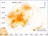 |
Fig. 11 Mosaic including all archival Chandra observations of the SNR MSH 11-61A and IGR J11014-6103 region. The dashed blue polygons are a reproduction of the extraction regions used by García et al. (2012) for the spectral analysis of the SNR (see discussion in Sect. 4). |
5. Conclusions
The overall structures of the PWN and main/counter-jet in the Lighthouse Nebula system are confirmed in the new deep Chandra observations. The PWN is now more clearly characterised as a wide flow up to 0.7′ from the pulsar and a more collimated region extended up to 1.7′, generally resembling the shape of an arrow. A clear softening of the spectrum along the PWN is observed and a nebular magnetic field of BPWN ≳ 30 μG is inferred.
The main jet still presents the same overall helical pattern seen in the previous Chandra observation, although several features at small and large scales cannot be fully explained in this model. A significant diffuse emission is detected around it, distributed asymmetrically with respect to the main jet axis. Different tentative interpretations of this outflow have been outlined. In particular, we analysed the scenario of a ballistic jet, possibly with kink instabilities, and the scenario of the diffusion of particles in the local ISM magnetic field. None, however, can reproduce satisfactorily all the observed spatial and spectral characteristics of the main jet, and the real nature of this feature remains to be investigated in greater detail.
The lack of H-α detection (given the presence of a strong surrounding nebulosity) and of detectable proper motion of the pulsar (given the short timescale spanned by the available data, and our distance from the system) are both compatible with the high linear speed (>1000 km s-1) derived previously for this pulsar.
For reference, at the distance of 7 kpc an angular scale of 1′ corresponds to ~2 pc.
See the Chandra documentation at http://cxc.harvard.edu/cal/ASPECT/celmon/
We included only sources within 8′ from the pulsar to avoid including boresite effects that are too strong.
In ciao/sherpa, the cstat implementation provides an approximate goodness of fit; the reduced statistic is approximately 1 for good fits.
The helical phase angle is computed from an arbitrary zero point.
PSR B0355+54 is travelling at only  km s-1 (Chatterjee et al. 2004), while IGR J11014-6103 is travelling at ~1000 km s-1.
A velocity of 1000 km s-1 – like that inferred for PSR J1101-6101 – is indeed considered a lower limit for a shock to start emitting X-rays.
Acknowledgments
The data analysed in this paper are based on Chandra and VLT observations obtained by our group. This research has made use of software provided by the Chandra X-ray Center (CXC) in the application packages CIAO, ChIPS, and Sherpa; the Heasarc ftools provided by NASA http://heasarc.gsfc.nasa.gov/ftools/Blackburn (1995); and the ATNF Pulsar Catalogue (Manchester et al. 2005). We thank M. Capasso, S. Fotopoulou, and C. Baldovin-Saavedra for useful discussions.
References
- An, H., Madsen, K. K., Reynolds, S. P., et al. 2014, ApJ, 793, 90 [NASA ADS] [CrossRef] [Google Scholar]
- Anders, E., & Grevesse, N. 1989, Geoch. Cosmoch. Acta, 53, 197 [Google Scholar]
- Appenzeller, I., Fricke, K., Fürtig, W., et al. 1998, The Messenger, 94, 1 [NASA ADS] [Google Scholar]
- Auchettl, K., Slane, P., Castro, D., Foster, A. R., & Smith, R. K. 2015a, ApJ, 810, 43 [NASA ADS] [CrossRef] [Google Scholar]
- Auchettl, K., Slane, P., Romani, R. W., et al. 2015b, ApJ, 802, 68 [NASA ADS] [CrossRef] [Google Scholar]
- Balucinska-Church, M., & McCammon, D. 1992, ApJ, 400, 699 [NASA ADS] [CrossRef] [Google Scholar]
- Balucinska-Church, M., & McCammon, D. 1998, ApJ, 496, 1044 [NASA ADS] [CrossRef] [Google Scholar]
- Bandiera, R. 2008, A&A, 490, L3 [NASA ADS] [CrossRef] [EDP Sciences] [Google Scholar]
- Begelman, M. 1998, ApJ, 493, 291 [NASA ADS] [CrossRef] [Google Scholar]
- Blackburn, J. K. 1995, in ASP Conf. Ser. 77, eds. R. A. Shaw, H. E. Payne, & J. J. E. Hayes (San Francisco: ASP), 367 [Google Scholar]
- Bogdanov, S. 2014, ApJ, 790, 94 [NASA ADS] [CrossRef] [Google Scholar]
- Bucciantini, N., Amato, E., & Del Zanna, L. 2005, A&A, 434, 189 [NASA ADS] [CrossRef] [EDP Sciences] [Google Scholar]
- Cappellari, M., & Copin, Y. 2003, MNRAS, 342, 345 [NASA ADS] [CrossRef] [Google Scholar]
- Chatterjee, S., & Cordes, J. M. 2002, ApJ, 575, 407 [NASA ADS] [CrossRef] [Google Scholar]
- Chatterjee, S., Cordes, J. M., Vlemmings, W. H. T., et al. 2004, ApJ, 604, 339 [NASA ADS] [CrossRef] [Google Scholar]
- Chatterjee, S., Vlemmings, W. H. T., Brisken, W. F., et al. 2005, ApJ, 630, L61 [NASA ADS] [CrossRef] [Google Scholar]
- Cordes, J. M., Romani, R. W., & Lundgren, S. C. 1993, Nature, 362, 133 [NASA ADS] [CrossRef] [Google Scholar]
- De Luca, A., Marelli, M., Mignani, R., et al. 2011, ApJ, 733, 104 [NASA ADS] [CrossRef] [Google Scholar]
- De Luca, A., Mignani, R. P., Marelli, M., et al. 2013, ApJ, 765, L19 [NASA ADS] [CrossRef] [Google Scholar]
- Eckert, D., Roncarelli, M., & Ettori, S. e. a. 2015, MNRAS, 447, 2198 [NASA ADS] [CrossRef] [Google Scholar]
- Erben, T., Schirmer, M., Dietrich, J. P., et al. 2005, Astron. Nachr., 326, 432 [NASA ADS] [CrossRef] [Google Scholar]
- Filipović, M., Payne, J., & Jones, P. 2005, Serb. Astron. J., 170, 47 [NASA ADS] [CrossRef] [Google Scholar]
- Fraix-Burnet, D. 1997, MNRAS, 284, 911 [NASA ADS] [CrossRef] [Google Scholar]
- Gaensler, B. 2005, Adv. Space Res., 35, 1116 [Google Scholar]
- Gaensler, B., Swaluw, E., Camilo, F., et al. 2004, ApJ, 616, 383 [NASA ADS] [CrossRef] [Google Scholar]
- García, F., Combi, J. A., Albacete-Colombo, J. F., et al. 2012, A&A, 546, A91 [NASA ADS] [CrossRef] [EDP Sciences] [Google Scholar]
- Giacinti, G., Kachelrieß, M., & Semikoz, D. V. 2013, Phys. Rev. D, 88, 023010 [NASA ADS] [CrossRef] [Google Scholar]
- Halpern, J. P., Tomsick, J. A., Gotthelf, E. V., et al. 2014, ApJ, 795, L27 [NASA ADS] [CrossRef] [Google Scholar]
- Hamuy, M., Walker, A. R., Suntzeff, N. B., et al. 1992, PASP, 104, 533 [NASA ADS] [CrossRef] [Google Scholar]
- Hamuy, M., Suntzeff, N. B., Heathcote, S. R., et al. 1994, PASP, 106, 566 [NASA ADS] [CrossRef] [Google Scholar]
- Harding, A. K., & Muslimov, A. G. 2011, ApJ, 743, 181 [NASA ADS] [CrossRef] [Google Scholar]
- Hobbs, G., Lorimer, D. R., Lyne, A. G., & Kramer, M. 2005, MNRAS, 360, 974 [NASA ADS] [CrossRef] [Google Scholar]
- Hui, C. Y., Huang, R. H. H., Trepl, L., et al. 2012, ApJ, 747, 74 [NASA ADS] [CrossRef] [Google Scholar]
- Janka, H.-T. 2012, Annu. Rev. Nucl. Part. Sci., 62, 407 [NASA ADS] [CrossRef] [Google Scholar]
- Johnson, S. P., & Wang, Q. D. 2010, MNRAS, 408, 1216 [NASA ADS] [CrossRef] [Google Scholar]
- Kamitsukasa, F., Koyama, K., Uchida, H., et al. 2015, PASJ, 67, 16 [NASA ADS] [Google Scholar]
- Kargaltsev, O., & Pavlov, G. G. 2008, AIP Conf. Proc., 983, 171 [Google Scholar]
- Kargaltsev, O., Cerutti, B., Lyubarsky, Y., & Striani, E. 2015, Space Sci. Rev., 191, 391 [NASA ADS] [CrossRef] [Google Scholar]
- Klingler, N., Kargaltsev, O., Rangelov, B., et al. 2016, ApJ, submitted [arXiv:1601.07174] [Google Scholar]
- Komissarov, S. S. 2013, MNRAS, 428, 2459 [NASA ADS] [CrossRef] [Google Scholar]
- Komissarov, S. S., & Lyubarsky, Y. E. 2004, MNRAS, 349, 779 [NASA ADS] [CrossRef] [Google Scholar]
- Lyubarskii, Y. E. 1999, MNRAS, 308, 1006 [NASA ADS] [CrossRef] [Google Scholar]
- Lyubarsky, Y. E. 2002, MNRAS, 329, 34 [Google Scholar]
- Lyutikov, M. 2006, MNRAS, 373, 73 [NASA ADS] [CrossRef] [Google Scholar]
- Manchester, R. N., Hobbs, G., Teoh, A., & Hobbs, M. 2005, AJ, 129, 1993 [NASA ADS] [CrossRef] [Google Scholar]
- Marelli, M., De Luca, A., Salvetti, D., et al. 2013, ApJ, 765, 36 [NASA ADS] [CrossRef] [Google Scholar]
- McGowan, K. E., Vestrand, W. T., Kennea, J. A., et al. 2006, ApJ, 647, 1300 [NASA ADS] [CrossRef] [Google Scholar]
- Moll, R. 2010, Ph.D. Thesis, Faculteit der Natuurwetenschappen, Wiskunde en Informatica [Google Scholar]
- Morlino, G., Lyutikov, M., & Vorster, M. 2015, MNRAS, 454, 3886 [NASA ADS] [CrossRef] [Google Scholar]
- Morris, M., Uchida, K., & Do, T. 2006, Nature, 440, 308 [NASA ADS] [CrossRef] [Google Scholar]
- Moser, A. L., & Bellan, P. M. 2012, Nature, 482, 379 [NASA ADS] [CrossRef] [Google Scholar]
- Motch, C., Pires, A. M., Haberl, F., Schwope, A., & Zavlin, V. E. 2009, A&A, 497, 423 [NASA ADS] [CrossRef] [EDP Sciences] [Google Scholar]
- Pavan, L., Bozzo, E., Pühlhofer, G., et al. 2011, A&A, 533, A74 (Paper I) [NASA ADS] [CrossRef] [EDP Sciences] [Google Scholar]
- Pavan, L., Bordas, P., Pühlhofer, G., et al. 2014, A&A, 562, A122 (Paper II) [NASA ADS] [CrossRef] [EDP Sciences] [Google Scholar]
- Reynoso, E. M., Johnston, S., Green, A. J., & Koribalski, B. S. 2006, MNRAS, 369, 416 [NASA ADS] [CrossRef] [Google Scholar]
- Rieger, F. M., Bosch-Ramon, V., & Duffy, P. 2007, Ap&SS, 309, 119 [NASA ADS] [CrossRef] [Google Scholar]
- Rossetti, M., Ghizzardi, S., Molendi, S., & Finoguenov, A. 2007, A&A, 463, 839 [NASA ADS] [CrossRef] [EDP Sciences] [Google Scholar]
- Schirmer, M. 2013, ApJS, 209, 21 [NASA ADS] [CrossRef] [Google Scholar]
- Slane, P., Chen, Y., Schulz, N. S., et al. 2000, ApJ, 533, L29 [NASA ADS] [CrossRef] [PubMed] [Google Scholar]
- Slane, P., Helfand, D. J., van der Swaluw, E., & Murray, S. S. 2004, ApJ, 616, 403 [NASA ADS] [CrossRef] [Google Scholar]
- Tang, X., & Chevalier, R. 2012, ApJ, 752, 83 [NASA ADS] [CrossRef] [Google Scholar]
- Tomsick, J. A., Bodaghee, A., Rodriguez, J., et al. 2012, ApJ, 750, L39 [NASA ADS] [CrossRef] [Google Scholar]
- Torii, K., Enokiya, R., Morris, M. R., et al. 2014, ApJS, 213, 8 [NASA ADS] [CrossRef] [Google Scholar]
- Van Etten, A., Romani, R. W., & Ng, C.-Y. 2012, ApJ, 755, 151 [NASA ADS] [CrossRef] [Google Scholar]
- Venter, C., Kopp, A., Harding, A. K., Gonthier, P. L., & Büsching, I. 2015, ApJ, 807, 130 [NASA ADS] [CrossRef] [Google Scholar]
- Wongwathanarat, A., Janka, H.-T., & Müller, E. 2013, A&A, 552, A126 [NASA ADS] [CrossRef] [EDP Sciences] [Google Scholar]
All Tables
Best fit parameters for the spectra of the different Lighthouse Nebula components.
All Figures
|
Fig. 1 Chandra 250 ks mosaic of the Lighthouse Nebula (exposure corrected and smoothed with a Gaussian kernel of σ = 1.5 pixel). The colour scale at the bottom of the plot is in units of photon/cm2/s. Solid red rectangles a–d (and the corresponding dashed background boxes) indicate the regions used to extract brightness profiles perpendicularly to the main jet (Sect. 2.3). The regions used for spectral extraction are also shown: the average spectra of the main jet, the counter-jet, and the PWN were extracted from the solid black regions (Sect. 2.4.1). For the point source PSR J1101-6101 we used a circle of radius 1.6′′ centred on the pulsar position (not shown). Background regions are marked with dashed black circles. In the inset: the details of the PWN shape and the attaching points of the two jets to the pulsar are visible. Coloured rectangles along the PWN indicate the regions used to extract spatially resolved spectra (Sect. 2.4.2). In this image, as in the rest of the paper, north is up and east is to the left. |
| In the text | |
|
Fig. 2 Mosaic image of IGR J11014-6103 with Voronoi adaptive binning. Each cell in this image has a S/N ≥ 3. The image is colour-coded in units of photon/cm2/s/arcmin2 as detailed in the colour map at the bottom of the plot. The pulsar, the main jet, the counter-jet, and the PWN are all detected at high significance. The broader emission around the main jet is also clearly detected. The black ruler shows linear distances along the jet. |
| In the text | |
|
Fig. 3 Top panels: brightness profile as a function of distance from the pulsar, extracted along the jets, from the regions shown in the image above (the brightness in the pulsar bin is not to scale). The horizontal scale is the same in the profile plot and in the extraction region image. The black profile is computed from the new 250 ks data; for comparison the profile obtained from the previous 50 ks observation is represented with a filled green histogram. Bottom panels: same as above, but for the extraction regions along the PWN. |
| In the text | |
|
Fig. 4 Surface brightness profiles (black histograms) extracted in four cuts perpendicular to the main jet (see regions a–d in Fig. 1). For comparison we also plot the corresponding profiles obtained from a model with a single narrow (green histogram) or large (green solid curve) helical jet (see Sect. 2.5). In each plot the distance from the jet axis increases towards the pulsar direction of motion (SW). |
| In the text | |
|
Fig. 5 Contour plots of the power-law fit parameters Γ and NH computed for the main jet (in blue) and the PWN (in red). Contours at 68%, 90%, and 99% confidence levels are shown for both cases. |
| In the text | |
|
Fig. 6 Photon index along the PWN (uncertainties at 1σ level). The best fit with a parabolic function is shown in red. |
| In the text | |
|
Fig. 7 Left panel: photon index map along the main jet and PWN. The colours represent different spectral indices, as shown in the colourbar at the bottom of the plot. Contours are drawn around the regions for clarity at levels of Γ = 1.1,1.5,1.8,2.8. Typical uncertainties on the spectral indices are of the order of ± 0.1. Right panel: the same contours are reported on the spatial map to aid the visual identification of the regions used for the spectral extractions and of the regions clustering around similar values of Γ. The region in red was used to extract spectra from the main jet. |
| In the text | |
|
Fig. 8 Upper panel: photon index Γ as a function of the distance along the collimated main jet (see extraction region in red in Fig. 7). Bottom panel: same as for the upper panel, but here plotted against flux in each Voronoi cell. |
| In the text | |
|
Fig. 9 Solid red line: best fit to the main jet with a simple helical model, superimposed on the 250 ks Chandra mosaic with Voronoi adaptive binning (Fig. 2). The model is in relatively good agreement with the shape of the jet at distances >90′′ from the pulsar; however, it fails to reproduce the regions closer to the pulsar and the counter-jet. Solid black lines represent tentative additional helices, each with a different helical phase. An additional tentative helix with different viewing angle is drawn with a dashed line. |
| In the text | |
|
Fig. 10 Lighthouse Nebula region in the H-α narrow band (continuum subtracted). Overplotted are the X-ray contours from the mosaic image in Fig. 1. At the bottom of PSR J1101-6101 a bright field star was masked with a MOS occulting bar. The diffuse emission is likely unrelated to the Lighthouse Nebula, and prevents detection of any possible emission from a bow-shock in front of PSR J1101-6101. |
| In the text | |
|
Fig. 11 Mosaic including all archival Chandra observations of the SNR MSH 11-61A and IGR J11014-6103 region. The dashed blue polygons are a reproduction of the extraction regions used by García et al. (2012) for the spectral analysis of the SNR (see discussion in Sect. 4). |
| In the text | |
Current usage metrics show cumulative count of Article Views (full-text article views including HTML views, PDF and ePub downloads, according to the available data) and Abstracts Views on Vision4Press platform.
Data correspond to usage on the plateform after 2015. The current usage metrics is available 48-96 hours after online publication and is updated daily on week days.
Initial download of the metrics may take a while.