| Issue |
A&A
Volume 591, July 2016
|
|
|---|---|---|
| Article Number | A73 | |
| Number of page(s) | 13 | |
| Section | Extragalactic astronomy | |
| DOI | https://doi.org/10.1051/0004-6361/201527647 | |
| Published online | 17 June 2016 | |
ALMA finds dew drops in the dusty spider’s web⋆
1 European Southern Observatory, Karl-Schwarzschild-Str. 2, 85748 Garching, Germany
e-mail: This email address is being protected from spambots. You need JavaScript enabled to view it.
2 Institut d’Astrophysique de Paris, UMR 7095, CNRS, Université Pierre et Marie Curie, 98bis boulevard Arago, 75014 Paris, France
3 Max-Planck-Institut für Extraterrestrische Physik, Giessenbachstraße 1, 85748 Garching, Germany
4 Centre for Extragalactic Astronomy, Department of Physics, Durham University, South Road, Durham DH1 3LE, UK
5 Université de Bordeaux, LAB, UMR 5804, 33270 Floirac, France
6 Universität Wien, Institut für Astrophysik, Türkenschanzstraße 17, 1180 Wien, Austria
7 Department of Earth and Space Science, Chalmers University of Technology, Onsala Space Observatory, 43992 Onsala, Sweden
8 Centro de Astrobiología (INTA-CSIC), Ctra de Torrejón a Ajalvir, km 4, 28850 Torrejń de Ardoz, Madrid, Spain
9 School of Physics and Astronomy, University of Nottingham, University Park, Nottingham NG7 2RD, UK
10 Institut d’Astrophysique Spatiale, CNRS, Université Paris-Sud, Bât. 120-121, 91405 Orsay, France
11 International Center for Radio Astronomy Research, Curtin University, GPO Box U1987, Perth, WA 6845, Australia
Received: 26 October 2015
Accepted: 10 February 2016
Abstract
We present 0.̋5 resolution ALMA detections of the observed 246 GHz continuum, [CI] 3P2→3P1 fine structure line ([CI]2–1), CO(7–6), and H2O lines in the z = 2.161 radio galaxy MRC1138-262, the so-called Spiderweb galaxy. We detect strong [CI]2–1 emission both at the position of the radio core, and in a second component ~4 kpc away from it. The 1100 km s-1 broad [CI]2–1 line in this latter component, combined with its H2 mass of 1.6 × 10¹⁰ M⊙, implies that this emission must come from a compact region <60 pc, possibly containing a second active galactic nucleus (AGN). The combined H2 mass derived for both objects, using the [CI]2–1 emission, is 3.3 × 10¹⁰ M⊙. The total CO(7–6)/[CI]2–1 line flux ratio of 0.2 suggests a low excitation molecular gas reservoir and/or enhanced atomic carbon in cosmic ray dominated regions. We detect spatially-resolved H2O 211−202 emission – for the first time in a high-z unlensed galaxy – near the outer radio lobe to the east, and near the bend of the radio jet to the west of the radio galaxy. No underlying 246 GHz continuum emission is seen at either position. We suggest that the H2O emission is excited in the cooling region behind slow (10–40 km s-1) shocks in dense molecular gas (103−5 cm-3). The extended water emission is likely evidence of the radio jet’s impact on cooling and forming molecules in the post-shocked gas in the halo and inter-cluster gas, similar to what is seen in low-z clusters and other high-z radio galaxies. These observations imply that the passage of the radio jet in the interstellar and inter-cluster medium not only heats gas to high temperatures, as is commonly assumed or found in simulations, but also induces cooling and dissipation, which can lead to substantial amounts of cold dense molecular gas. The formation of molecules and strong dissipation in the halo gas of MRC1138-262 may explain both the extended diffuse molecular gas and the young stars observed around MRC1138-262.
Key words: galaxies: evolution / galaxies: high-redshift / galaxies: active / galaxies: ISM / Galaxy: halo
The reduced data cubes are only available at the CDS via anonymous ftp to cdsarc.u-strasbg.fr (130.79.128.5) or via http://cdsarc.u-strasbg.fr/viz-bin/qcat?J/A+A/591/A73
© ESO, 2016
1. Introduction
The high-z radio galaxy (HzRG) MRC1138-262 at z = 2.161 is one of the best studied HzRG (e.g. Pentericci et al. 1997, 1998, 2000; Carilli et al. 1997, 2002; Stevens et al. 2003; Kurk et al. 2004b,a; Greve et al. 2006; Miley et al. 2006; Hatch et al. 2008, 2009; Humphrey et al. 2008; Kuiper et al. 2011; Ogle et al. 2012; Seymour et al. 2012), with a well sampled spectral energy distribution (SED) that covers from radio to X-ray. Its radio morphology is typical of distant radio galaxies with a string of radio bright knots along the radio jet that extends to the west and a single lobe to the east of the central radio core (Carilli et al. 1997). The radio core has an “ultra steep” spectral index of α = −1.2, and the spectral indices of the radio knots systematically steepen with increasing distance from the core (Pentericci et al. 1997).
The radio source is embedded in an environment that is over-dense in galaxies, over scales of hundreds of kpc (Pentericci et al. 1998; Miley et al. 2006) to Mpc scales (Pentericci et al. 2002; Kurk et al. 2004b,a; Dannerbauer et al. 2014). Many of these galaxies are clumpy and star-forming (Pentericci et al. 1998; Miley et al. 2006; Dannerbauer et al. 2014). Hatch et al. (2009) predict that most of the satellite galaxies within 150 kpc will merge with the central HzRG and that the final merger galaxy will contain very little gas owing to the high star formation rate (SFR) of the satellite galaxies. X-ray observations of MRC1138-262 are inconclusive about the existence of an extended X-ray atmosphere (cf. Carilli et al. 2002; Pentericci et al. 2000, the extended X-ray emission could be due to inverse Compton or shocks generated by the passage of the radio jets). Pentericci et al. (2000), who favour the existence of a large thermal hot X-ray emitting atmosphere, conclude that MRC1138-262 has many of the necessary ingredients of a forming galaxy cluster, i.e. an irregular velocity distribution of the Ly α emitting galaxies, an over-density of galaxies, a massive central galaxy, and a hot X-ray halo. Owing to the large number of companion galaxies surrounding the HzRG being analogous to “flies caught in a spiders web”, MRC1138-262 was dubbed the Spiderweb galaxy (Miley et al. 2006).
Multi-wavelength photometry, including the infrared continuum emission (Stevens et al. 2003; Greve et al. 2006; De Breuck et al. 2010), implies an extremely high SFR in the Spiderweb galaxy. Fitting an active galactic nucleus (AGN) and starburst component SED to the mid- to far-IR SED, Seymour et al. (2012) find a SFR for the starburst component of 1390 ± 150 M⊙ yr-1 (see also Ogle et al. 2012). This should be compared with the rest-frame UV estimates of only a couple 100 M⊙ yr-1 (even with an extinction correction) by Hatch et al. (2008), who emphasise how deeply embedded the majority of the intense star formation is in MRC1138-262. Although the star formation is intense, the characteristics of the vigorous outflow (Ṁ ≳ 400 M⊙ yr-1) that is observed in the optical emission line gas suggest that this is predominately driven by the radio jet (Nesvadba et al. 2006).
Beyond the companion galaxies of the HzRG, the diffuse stellar and gaseous environment of MRC1138-262 on larger scales is also fascinatingly complex. MRC1138-262 has a significant amount of diffuse UV intergalactic light (IGL) within 60 kpc of the radio galaxy, which indicates ongoing star formation in the circumgalactic environment (Hatch et al. 2008). This diffuse light is embedded in a large (~100 kpc in diameter) Lyα emitting halo (Pentericci et al. 1997). Using semi-analytical models, Hatch et al. (2008) ruled out the possibility that the observed circumgalactic light originates from unresolved, low-mass satellite galaxies. Spectra extracted at the position of the central HzRG, of a nearby galaxy and the IGL, show Ly α emission lines with absorption troughs superimposed, which suggests the presence of warm neutral gas mixed with the ionised gas that surrounds the HzRG (Pentericci et al. 1997; Hatch et al. 2008). This leads to the conclusion that the large Ly α halo emission is powered not only by the extended and diffuse star formation (Pentericci et al. 1998; Miley et al. 2006; Hatch et al. 2008) but also by AGN photoionisation and shock heating (Nesvadba et al. 2006).
The influence of the radio jet from the AGN is seen in the VLA observations, which reveal a bend in the western string of clumps detected ~20 kpc from the core towards the south-west. Ly α line emitting gas has a bright spot associated with this bend and the two hotspots, implying the presence of a massive cloud of gas deflecting the radio jet and causing these features (Pentericci et al. 1997; Lonsdale & Barthel 1986). Several different models exist for how gas might deflect radio jets, such as the jet drilling into a gas cloud where it blows a bubble in the hot plasma (Lonsdale & Barthel 1986) or through the counter pressure generated by oblique reverse shocks in the cloud generated by a jet-cloud interaction (Bicknell et al. 1998). Given this situation, Pentericci et al. (1997) argue that the relation between the radio emitting knots in the jet and the high surface brightness Ly α halo emission, especially where the eastern jet bends, suggest an interaction between the jet and the ambient gas in the halo of MRC1138-262. However, the origin of the Ly α emitting gas reservoir is still uncertain.
This high an SFR of the HzRG means that a significant molecular gas reservoir fuelling the star formation must be present. Emonts et al. (2013) probe the diffuse extended molecular gas reservoir using the CO(1–0) line. They find that there is approximately 6 × 10¹⁰M⊙ of cold H2 gas over a scale of 10 s of kpc, which surrounds the HzRG (also Emonts et al., in prep.). The kinematics of the cold molecular gas is relatively quiescent (Emonts et al., in prep.). More surprisingly, Ogle et al. (2012) detect the 0-0 S(3) rotational line of H2 in MRC1138-262. The strength of the line, allowing for a range of plausible excitation temperatures of H2, imply warm (T> 300 K) H2 masses of order 107 to 109M⊙. While the large Spitzer beam does not allow the H2 emission to be spatially resolved, a plausible interpretation of the relatively large mass of warm H2 gas in MRC1138-262 is that a fraction of the jet energy is being dissipated as supersonic turbulence and shocks in the dense gas in the immediate environment of the AGN.
Although the optically thick CO(1–0) emission line is a good tracer of the diffuse molecular gas, the emission lines from neutral carbon ([CI]) are arguably even better. The [CI] lines have critical densities similar to the low-J CO lines, meaning that they probe the same phases of the molecular gas. As they are both optically thin, they therefore probe higher column densities than CO (Papadopoulos et al. 2004). While the [CI] lines are good tracers of the diffuse molecular gas, they are poor tracers of the very dense star-forming gas. Molecular lines from, for example, H2O, HCN, and CS have a much higher critical density, and therefore probe the dense molecular star-forming phase. Omont et al. (2013) find a relation between the far-infrared (FIR) and H2O luminosities for a sample of high-z starburst galaxies. The H2O detections for this sample are all associated with underlying FIR emission, implying that the H2O emission traces star-forming regions. However, the H2O molecules can also be excited in the dissipation of supersonic turbulence in molecular gas or by slow shocks (e.g. Flower & Pineau Des Forêts 2010). In the case of purely shock-excited H2O, it is unlikely that underlying FIR emission would be detected in regions of strong H2O emission (e.g. Goicoechea et al. 2015).
Motivated to determine the energy source and distribution of the strong dissipation as possibly observed through H2 emission and to determine the state of the molecular gas in MRC1138-262, we proposed for ALMA observations in Cycle 1. In this paper, we present our results for the observed 246 GHz continuum emission (rest-frame ~740 GHz), H2O 211−202 transition (at νrest = 752.03 GHz, which hereafter is often referred to as H2O), [CI] 3P2→3P1 fine structure emission line (at νrest = 809.34 GHz, which hereafter is referred to as [CI]2–1), and CO(7–6) emission line observations towards the Spiderweb galaxy. We find strong 246 GHz continuum emission at the position of the HzRG. Near both radio lobes, we detect emission from H2O, the first spatially resolved detection of H2O in a high-z unlensed galaxy. We also detect strong [CI]2–1 emission that is blended with weak CO(7–6) emission at the position of the HzRG. In Sect. 2, we present our Atacama Large Millimeter/submillimeter Array (ALMA) submm observations. The results of these observations are given in Sect. 3. We analyse and discuss them in Sect. 4 and summarise our conclusions in Sect. 5. We assume H0 = 73 km s-1 Mpc-1, ΩM = 0.27, and ΩΛ = 0.73, which implies a scale of 8.172 kpc/′′ at z = 2.161.
2. Observations
2.1. ALMA observations
The ALMA cycle 1 Band 6 observations were carried out on 2014 April 27 for 49 min on-source time with 36 working antennas. The four 1.875 GHz spectral windows were tuned to cover the frequency ranges 237.3−240.9 GHz and 252.6−256.7 GHz. We used the supplied Common Astronomy Software Applications (CASA) calibration script to produce the data cube, continuum map, and moment-0 maps. The quasar J1146-2859 was used as a bandpass calibrator, and the UV range was well covered within 400 kλ.
We made a natural weighted map (Briggs robust parameter of 2), which exhibits the highest signal-to-noise ratio (S/N), at the expense of a lower spatial resolution. The frequency range between 254.9−265.7 GHz (i.e. half of the upper side band) is dominated by strong [CI]2–1 and CO(7–6) line emission and is therefore not included in the continuum map. This results in a continuum map with a synthesised beam of  with PA 89.3° and a root mean square (rms) of 50 μJy/beam. We corrected the continuum map for the primary beam of 26.̋3.
The H2O emission is spatially offset from the continuum emission and a continuum subtraction is therefore not required, as it would only, unnecessarily, add noise. The H2O observations are therefore not continuum-subtracted. The [CI]2–1 and CO(7–6) emission lines are within the frequency range at z = 2.1606, and we subtract the continuum in the UV-plane by fitting a first order polynomial to the line free channels. The [CI]2–1 emission is so broad that it leaves no line-free channels in spectral window 0. We therefore fit the continuum to spectral window 1, which shows no signs of line emission. We bin the [CI]2–1 line data to 20 km s-1, which has an rms of 0.5 mJy and the H2O line data to 60 km s-1, which has an rms of 0.3 mJy. We primary beam-correct the H2O line data, since we find H2O emission ~6 from the phase centre, where the sensitivity is at 87%.
3. Results
The Spiderweb galaxy is detected in both 246 GHz continuum and [CI]2–1, CO(7–6) and H2O line emission. Figure 1 shows an overview of the spatial distribution of the different components. The strong [CI]2–1 line emission is seen in two components that are separated by 0.̋5. The [CI]2–1 component 1 is centred at the position of the HzRG (shown with a blue ellipse in Fig. 1) and the [CI]2–1 component 2 is located 0.̋5 to the south-east (shown with a red ellipse in Fig. 1). The 246 GHz continuum emission peaks at the position of the HzRG (shown with green ellipses in Fig. 1), but shows an extension in the direction of the [CI]2–1 component 2. Emission from H2O is also detected south-west of the HzRG (shown with the orange ellipse, south of the 246 GHz continuum component in Fig. 1), which is co-spatial with the bend in the radio jet (Carilli et al. 1997). H2O emission is detected east of the HzRG – west of knot A in the radio jet (shown with an orange ellipse to the left, in Fig. 1). We now discuss each of the components separately. Table 2 lists the derived line parameters. Throughout, we adopt the [CI]2–1 emission at the position of the radio core as the systemic redshift z = 2.1606.
3.1. Continuum emission
The continuum map contains bright 246 GHz continuum emission at the position of the HzRG, ~20 kpc to the west and tentative emission to the north (see Fig. 1).
3.1.1. The HzRG
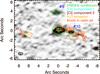 |
Fig. 1 Overview of the spatial distribution of the detected components. The naturally weighted 246 GHz continuum map is in greyscale and the two [CI]2–1 components, 1 and 2, are shown with blue and red ellipses, respectively. The two H2O detections are shown with orange ellipses, and the 246 GHz continuum components shown with green ellipses. The sizes of the ellipses represent the extractions used for the photometry. The knots in the radio jet are indicated with red-orange diamonds and labeled according to Pentericci et al. (1997). The numbers correspond to the numbering in Kuiper et al. (2011). The ALMA beam is shown as a black ellipse in the lower left corner. |
The 246 GHz continuum emission at the position of the HzRG shows an east-west elongation, in the same orientation as the radio source (see Fig. 1). A similar orientation was seen in the SCUBA and LABOCA maps (Stevens et al. 2003; Dannerbauer et al. 2014), but those extensions were on a much larger scale than the separation seen in Fig. 1. Although the continuum only has one peak, the elongation suggests a two component system, similar to that seen in the [CI]2–1 line emission (see Sect. 3.2.1). Using the peak positions from component 1 and 2 in the [CI]2–1 moment-0 maps, we fit a double 2D Gaussian profile to the continuum by fixing the centres of the Gaussians at the peak positions of the [CI]2–1 emission line. This results in a continuum ratio for the two components of ~5. Integrating the fitted double 2D Gaussian yields the flux density of 1.78 ± 0.29 mJy (see Table 1). This emission is probably dominated by thermal dust emission, although we warn that a linear extrapolation of the S(8.2 GHz) = 1.88 mJy (Pentericci et al. 1997) and the S(36.5 GHz) = 1.02 mJy (Emonts et al., in prep.) for the core predicts a synchrotron contribution of 0.47 mJy at 246 GHz. Any star formation parameters derived directly from the 246 GHz should therefore be considered as an upper limit.
Peak positions and 246 GHz continuum flux of the HzRG and companion #8 and #10.
3.1.2. The companion sources
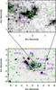 |
Fig. 2 Bottom panel: HST F814W image (Hatch et al. 2008) in greyscale overlaid with the naturally weighted 246 GHz continuum map in green contours with levels of 1.5σ, 3σ, and 5σ. In the naturally weighted continuum map, we detect emission from companion #10 (and tentatively from #8) of Kuiper et al. (2011). The purple cross indicate the position of the nearby Ly α emitter at the position of the HzRG. The purple circles indicate the positions of Ly α emitters, the squares show the position of Hα and the triangles extremely red objects within the Ly α halo of MRC1138-262. The Ly α emitter #491 is offset by 0.̋8 from the companion source seen in the 246 GHz continuum emission west of the HzRG. Top panel: zoom in of the region around the companion sources. The purple circle shows the position of the Hα emitter #491 (Kurk et al. 2004b), which is close to the companion source seen in dust continuum emission. |
We detect 246 GHz continuum emission from a bright companion ~20 kpc to the west of the HzRG (see Fig. 1). This companion is associated with knot B3 in the radio jet (Carilli et al. 1997; Pentericci et al. 1997, see Fig. 1) and a small group of galaxies (denoted D by Pentericci et al. 1997, and #10 by Kuiper et al. 2011, see Fig. 2). This is also the position of a high surface brightness region of Lyα emission (Pentericci et al. 1997). This companion is also seen in, for example, HST F814W imaging (Miley et al. 2006) and at other optical wavelengths, e.g. R-band (Pentericci et al. 1997). Companion #10 is co-spatial with companion D in Pentericci et al. (1997) at RA = 11:40:48.14, Dec = −26.29.09.2, and is offset by only 0.̋8 to the Ly α emitter #491 from Kurk et al. (2004b). This Ly α emitter at RA = 11:40:48.2, Dec = −26.29.09.5 (shown with the purple circle in Figs. 2) is inside the Ly α halo of the Spiderweb galaxy (Kurk et al. 2004b), and so are three other Ly α emitters, three Hα emitters, and two extremely red objects (ERO, also indicated in Fig. 2). Fitting a 2D Gaussian profile to companion #10, we find a flux density of 0.19 ± 0.01 mJy (see Table 1).
To examine the nature of the 246 GHz emission of companion #10, we compared the flux density in the spectral windows that were not contaminated by line emission. The expected ratio between 238.28 and 253.48 GHz (i.e. the lower and upper side bands: LSB and USB) from thermal blackbody radiation at 40 K is 0.80, while the observed ratio is 1.19 ± 0.22. The Decreasing spectral slope with increasing frequency of #10 is more consistent with a synchrotron rather than a thermal dust origin. Indeed, a straight extrapolation of the S8.2 GHz = 5.9 mJy (Pentericci et al. 1997) and the S36.5 GHz = 1.8 mJy (Emonts et al., in prep.) implies S239 GHz = 0.4 mJy. Our observed 0.2 mJy is therefore fully consistent with synchrotron emission, and even allows for the expected spectral steepening at high frequencies. Thus synchrotron-dominated submm emission is consistent with companion #10 having very blue UV colours with no signs of a Balmer break or significant extinction (Hatch et al. 2009). On the other hand, it could also be that the most obscured regions are not visible in the optical images, but only the bluest, least obscured regions are. Higher resolution dust continuum and a broad sub-millimetre wavelength coverage can test these hypotheses.
3.2. [CI]2–1 and CO(7–6) line emission
3.2.1. The HzRG
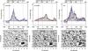 |
Fig. 3 [CI]2–1 spectra and moment-0 maps for component 1, component 2, and the total [CI]2–1 and CO(7–6) emission. Top row: the spectra extracted from beam-sized areas for component 1, component 2, and the total. The areas from which the spectra of component 1 and component 2 are extracted do not overlap. The Lorentzian profile for the component 1 [CI]2–1 line (top left), the double Gaussian profile for the component 2 [CI]2–1 line (top middle), and the single Gaussian fits for the two CO(7–6) lines are over-plotted as black curves. The sum of the Lorentzian and Gaussian profiles is over-plotted in black in the total spectrum (top right). The dashed lines indicate the 0-velocity of the [CI]2–1 frequency at z = 2.1606, and the dotted lines indicate the 0-velocity for the CO(7–6) frequency at the same redshift. This redshift is in agreement with the redshift determined from the CO(1–0) line (Emonts et al. 2013). The dotted-dashed line indicate the 0-velocity of the [CI]2–1 frequency at z = 2.156, determined from the HeII λ1640Å line (which, as a non-resonant line, should represent the systemic velocity of the AGN, Humphrey et al. 2008). Bottom row: the moment-0 maps of the [CI]2–1 emission from component 1 (bottom left), component 2 (bottom middle), and the total (bottom right) [CI]2–1 emission and zoom-ins of the centres of the images. The total [CI]2–1 moment-0 maps is overlaid with [CI]2–1 line contours of component 1and 2. The blue and red crosses indicate the peaks of the [CI]2–1 emission of component 1 (blue) and component 2 (red). |
Strong emission from the [CI] 3P2 → 3P1 fine structure emission line is detected at the position of the HzRG. The [CI]2–1 emission line has a double peaked velocity profile with peaks at 0 km s-1 and ~350 km s-1 (see top right in Fig. 3). Moment-0 maps of the channels containing the emission of the first (see bottom left in Fig. 3) and second (see bottom middle in Fig. 3) peaks reveal a spatial mis-alignment of the two [CI]2–1 peaks, which suggests two components. The emission that corresponds to the 0 km s-1 peak is at the location of the HzRG (component 1, indicated with a blue cross in Fig. 3), while the ~350 km s-1 gas is shifted 0.̋5 to the south-east (component 2, indicated with the red cross in Fig. 3). A broad underlying component is visible in the spectrum for component 2. Unfortunately, the spatial resolution of the data and the broad underlying component do not allow for a clearer separation of the two components.
The spectral velocity profile of component 1, with no overlap with component 2 (see Fig. 3 left), has a Lorentzian-shaped profile, with a full-width at half-maxima (FWHM) of 270 ± 15 km s-1 and a redshift of z = 2.1606 ± 0.0041, which agrees with the redshift determined from the CO(1–0) line (Emonts et al. 2013). We adopt this as the systemic redshift since the [CI]2–1 line has higher spectral resolution and S/N compared to the HeII λ1640 Å (Hatch et al. 2008). At the expected frequency of the CO(7–6) line, we detect a 3.5σ Gaussian shaped CO(7–6) emission line with FWHM of 435 ± 85 km s-1. The broadness of the [CI]2–1 line makes the spectroscopic separation of the [CI]2–1 and CO(7–6) lines difficult, as very few line-free channels separate them. To avoid the lines contaminating each other, the velocity integrated line flux for the [CI]2–1 line is calculated by integrating the fitted profile from −610 km s-1 to 530 km s-1, while the integrated CO(7–6) line flux is integrated from 690 km s-1 to 1390 km s-1. The CO(7–6) to [CI]2–1 line luminosity ratio is 0.2. The peak ratio of the two [CI]2–1 components is ~3 times lower than the ratio of the 246 GHz continuum at these positions, implying that component 2 is relatively brighter in [CI]2–1 than in 246 GHz emission.
The velocity profile of component 2 shows evidence for two components, one broad and one much narrower component (see Fig. 3). The best two-component Gaussian fit has a FWHM of 1100 ± 65 km s-1 for the broad, and 230 ± 35 km s-1 for the narrow components. The centre of the narrow component is shifted ~360 km s-1 redward of the systemic velocity of the [CI]2–1 line for component 1. The CO(7–6) emission line is also detected for component 2, at a level of 4.8σ, which is more significant than the CO(7–6) detection for component 1. The CO(7–6) line peaks at ~1275 km s-1 relative to the centre of the [CI]2–1 line, corresponding to a rest velocity for the CO(7–6) line of ~280 km s-1. The narrow component of the [CI]2–1 line and the CO(7–6) line both have an offset of 80 km s-1 relative to the systemic redshift of component 1. Just as for component 1, separating the two lines spectroscopically is difficult and we therefore calculate the integrated flux of the [CI]2–1 line from −825 km s-1 to 990 km s-1 and the integrated flux of the CO(7–6) line from 1000 km s-1 to 1490 km s-1. We additionally derive the flux of the narrow and broad components separately, by integrating the fitted Gaussian profiles. The CO(7–6) to [CI]2–1 line luminosity ratio is 0.14, lower than for component 1. The two components have a [CI]2–1 line peak ratio of 1.7, and a CO(7–6) line peak ratio of 0.4.
The total spectrum of the two components (see Fig. 3 right) clearly shows a double peaked [CI]2–1 line and a broad CO(7–6) line. We sum the Lorentzian fit of component 1 and the two Gaussian fits of component 2, which results in a profile that fits the observed integrated [CI]2–1 line of both components well. We likewise sum the two single Gaussians fitted to the CO(7–6) lines in component 1 and component 2. The full [CI]2–1 plus CO(7–6) profile is over-plotted on the full spectrum in the top right panel of Fig. 3. The CO(7–6) line in the total spectrum is even broader than for component 1 and 2, making the separation even more difficult. We therefore calculate the [CI]2–1 integrated line flux from −590 km s-1 to 700 km s-1 and the CO(7–6) integrated line flux is integrated from 700 km s-1 to 1390 km s-1. The CO(7–6) to [CI]2–1 line luminosity ratio for the total spectrum is 0.2, the same as for component 1.
3.2.2. The companion source
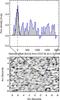 |
Fig. 4 Bottom panel: moment-0 map of the CO(7–6) emission at the position of the brightest companion. Top panel: spectrum extracted from the beam-size area shown by the blue ellipse at the position of the companion sources in the bottom panel and is binned to 30 km s-1 channels. The spectrum shows both the continuum and CO(7–6) line emission. The redshift of the line is consistent with the optical z = 2.1446 (Kuiper et al. 2011), which was taken as zero velocity in the spectrum. |
We detect line emission in companion #10 ~20 kpc to the west of the HzRG (see Fig. 4). SINFONI spectroscopy of this companion shows line emission from Hα, [OII] and [OIII], and that companion #10 has a velocity offset of ~−1360 km s-1, which corresponds to a redshift of z = 2.1446 (Kuiper et al. 2011). Unfortunately, the [CI]2–1 is shifted out of the observed band at this redshift and the H2O line falls in a gap in the response of the band. However, the CO(7–6) line is offset by 997 km s-1 from the [CI]2–1 line and therefore still lies within the band at this redshift. We identify the detected emission line as CO(7–6) line emission from companion #10 (see Fig. 4). It is therefore highly likely that the 246 GHz continuum emission that we detect at this position is related to companion #10. This CO(7–6) line can be fitted with a Gaussian profile with a FWHM of 130 ± 20 km s-1 and the integrated line flux from − 170 km s-1 to 150 km s-1 of 0.08 ± 0.01 Jy km s-1 (Table 2). We do not detect any line emission at the position of the tentative 246 GHz continuum companion #8.
H2O, [CI]2–1 and CO(7–6) emission line positions, velocity integrated fluxes, and FWHMs.
3.3. H2O line emission
We detect emission from the H2O 211−202 transition ~25 kpc to the west and ~50 kpc to the east of the radio core at the expected observed frequency for H2O at z = 2.1606. The western 4σ detection is located just south of the strongest 246 GHz continuum companion, at the bend of the radio jet, i.e. at radio knot B4 (see Fig. 5). The eastern 3.7σ detection is located west of the radio knot A (see Fig. 5). To establish that this emission is real, we perform a Jackknife test, cutting the observed time in half. The two H2O lines show up in both halves of the data with a ≳2σ significance, which suggests that the emission lines are real and not simply noise peaks. Fitting Gaussian profiles to the emission lines result in FWHMs and relative velocities of 230 ± 50 and 160 ± 20 km s-1 for the western detection and 350 ± 70 and 125 ± 30 km s-1 for the eastern detection respectively. No 246 GHz continuum emission is detected at the positions of the two H2O detections down to an rms of 40 μJy, and no H2O emission line is detected at the position of the HzRG (see Fig. 5) down to an rms of 40 μJy in 60 km s-1 wide channels; assuming that the 720 km s-1 width of the CO(7–6) line from the total spectrum yields a 3σ upper limit of 0.9 Jy km s-1.
4. Analysis and discussion
The lines we detected in the Spiderweb galaxy are useful for a wide range of gas diagnostics. The atomic forbidden line of carbon, [CI]2–1, is a good tracer of relatively diffuse, low extinction molecular gas (e.g. Papadopoulos et al. 2004), since its line strength is linearly proportional to the column density of molecular gas (Glover et al. 2015). CO(7–6) emission is strong in dense, highly excited optically thick molecular gas. The thermal dust continuum over the range of a few 100 GHz represents the cooling of dust that is heated by the intense stellar and AGN radiation fields within the Spiderweb galaxy. The H2O 211−202 line is excited either in slow shocks (10−40 km s-1) in dense molecular gas (103−5 cm-3; Flower & Pineau Des Forêts 2010) or by IR pumping (e.g. van der Werf et al. 2011). Thus our data, in principle, probe a wide range of conditions and heating/excitation mechanisms in (relatively dense) molecular and atomic gas.
4.1. Diffuse and dense molecular gas
4.1.1. Line velocity profiles
Fitting of Lorentzian and Gaussian profiles for the emission line shows that the [CI]2–1 and CO(7–6) lines component 1 and 2 have very different velocity profiles. Figure 6 compares the velocity profiles of the [CI]2–1 and CO(7–6) emission lines for component 1 (left), component 2 (middle), and the total (right). Both the [CI]2–1 and CO(7–6) emission lines of component 1 are broad, but though [CI]2–1 and CO(7–6) do not trace exactly the same phases of the molecular gas, the broadness of the two lines does suggest that the two phases are related. The velocity profiles of the [CI]2–1 and CO(7–6) lines for component 2 show similarities between the narrow [CI]2–1 component and the CO(7–6) line. The broad [CI]2–1 component is not seen in the CO(7–6) line because of both the limited spectral coverage of our observations on the high velocity end of our bandpass, and limited S/N of this faint line. The fact that the narrow velocity gas in component 2 is detected in both [CI]2–1 and CO(7–6) emission and with similar FWHM indicates that this is a well-defined object. High spatial resolution observations would be required to determine if this is a separate self-gravitating object, or a kinematic feature within the same physical object. The broadness of the CO(7–6) emission in the total spectrum indicates that this emission is dominated by the CO(7–6) emission from component 1.
The CO(7–6) lines for both component 1 and 2, show an offset from the systemic redshift of ~90–100 km s-1. A similar offset between the [CI] and CO lines is seen in a study of H1413+117 (the Cloverleaf Galaxy) by Weiß et al. (2003). They conclude that the reason for the shift is unclear, but that gravitational amplification should not alter the frequency of the lines, unless the distribution of the [CI] and CO emitting gas is different. Because the [CI] and CO lines for the Cloverleaf Galaxy have low S/N, Weiß et al. (2003) conclude that high S/N observations are necessary to confirm the offset and its origin, but that, if it is genuine, it is most likely due to opacity effects. Since we see a similar offset for the Spiderweb galaxy, which is an unlensed source, differential lensing cannot be the cause of this offset, however, differences in the opacity of the two lines f. The CO(7–6) line has a higher optical depth than the [CI]2–1 line (τ[ CI ] = 0.1, Weiß et al. 2003), meaning that the CO(7–6) emitted photons go through internal absorption and emission. The line photons, whose frequencies have been shifted away from the systemic frequency of the CO(7–6) emission line, have a higher probability of escaping, thus shifting the overall observed frequency.
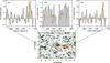 |
Fig. 5 Non-continuum subtracted H2O spectra for the detection of the west and east and the non-detection at the position at the HzRG and H2O moment-0 map. Top left panel: H2O line detected ~50 kpc to the east of the radio core, has a 3.7σ significance. The emission is located due west of the knot A in the radio jet. The fitted Gaussian is over-plotted in orange. Top middle panel: spectrum at the position of the radio core, shows no detection of H2O emission – only continuum emission. A small separation between the two spectral windows results in the gap in the continuum between − 1300 and − 1500 km s-1. Top right panel: H2O line detected ~25 kpc to the west of the radio core, showing a 4σ H2O detection at the expected frequency for z = 2.161. The emission is located at the bend of the radio jet, B4 (Pentericci et al. 1997). The best-fit Gaussian is over-plotted in orange. Bottom panel: moment-0 map of the H2O emission (without continuum subtraction), overlaid with the 246 GHz continuum emission in green contours. The orange ellipses show the H2O emission and the orange-red diamonds the positions of the knots in the radio jet, given by Pentericci et al. (1997). |
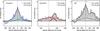 |
Fig. 6 [CI]2–1 spectra (dark blue, dark red and black histograms) for component 1, component 2, and the total over-plotted with the respective CO(7–6) lines (light blue, orange and white histograms) to compare the velocity profiles. The fitted profiles from Sect. 3 are over-plotted as black curves, with the individual velocity components as dotted lines. The narrow [CI]2–1 component of component 2 is offset by 365 km s-1 from the systemic redshift. The bar above the velocity profiles in the right plot, marked the HeII redshift and errors (olive bar) from Röttgering et al. (1997) and the CO(1–0) redshift and error (blue bar) from Emonts et al. (2013). |
The Hα line for the Spiderweb galaxy was detected with SINFONI (Nesvadba et al. 2006) and ISAAC (Humphrey et al. 2008). The Hα (λ 6550), [NII] (λ 6585) lines, and [SII] (λλ 6718, 6733) doublet are spectrally very close and the lines are therefore blended together. Both studies fit the blended lines with multiple Gaussians. Nesvadba et al. (2006) finds FWHM = 14 900 km s-1 for the AGN component and FWHM< 2400 km s-1 for the emission originating from a region that surrounds the AGN. This is the same order of magnitude that Humphrey et al. (2008) find by fitting six Gaussian profiles, including two Hα components. These two Hα components consist of a transmitted broad line region from the AGN (FWHM = 13 900 ± 500 km s-1), and a component with FWHM = 1200 ± 80 km s-1. The relatively low spectral resolution of the ISAAC spectrum does not allow for a further de-blending of the lines. However, the Hα line profile does show the presence of a broad and narrow component, similar to what we observe in the [CI]2–1 emission of component 2. This strengthens the idea that the [CI]2–1 emission traces the bulk of the gas in the galaxy, which is consistent with the [CI] emitting gas being distributed throughout and, generally, tracing gas of moderate extinctions and relatively low density molecular gas (Papadopoulos et al. 2004).
4.1.2. Line ratios
SMGs and QSOs from the literature with published [CI]2–1, CO(7–6) and H2O detections along with published IR luminosities used for comparison to the Spiderweb galaxy.
The utility of using the [CI] emission lines as tracers of the H2 column density has been examined by Papadopoulos et al. (2004) by considering the [CI]2–1 to CO line ratio. The [CI] lines, [CI]3P P0 ([CI]1–0) and [CI] 3P
 P1 ([CI]2–1), have critical densities of ncr, [ CI ] 1 - 0 ~ 500 cm-3 and ncr, [ CI ] 2 - 1 ~ 103 cm-3, similar to that of CO(1–0) and CO(2–1), which are often used as H2 tracers. The [CI] lines have low to moderate optical depths (τ ≈ 0.1−1), which means that these lines have the advantage, compared to CO, of tracing higher column-density cold diffuse molecular gas. The [CI] lines are also more easily excited. These properties make the [CI] lines more direct tracers of the molecular gas mass than the optically thick 12CO lines. Though the H2-tracing capability of [CI] decreases for low metallicities, Papadopoulos et al. (2004) conclude it is still a better H2 tracer than 12CO (see also Glover et al. 2015).
The ground-state transition, [CI]1-0, is the most direct H2 gas-mass tracer of the two [CI] lines because it is (relatively) less sensitive to the excitation conditions of the gas. However, the [CI]2–1 is still a much better tracer of the H2 gas than the CO(7–6) line at a similar frequency. The much higher critical density of the CO(7–6) line of ncr,CO(7 - 6) ~ 3 × 106 cm-3 and higher excitation energy of E76/k ~ 155 K, compared to E21/k ~ 62 K for the [CI]2–1 line, means that the [CI]2–1 and CO(7–6) lines are unlikely to trace exactly the same molecular gas phases. The CO(7–6) line is likely tracing the higher density, more highly excited molecular gas.
We searched the literature for high-z sources with observations of both the [CI]2–1 and CO(7–6) emission lines and determined IR luminosities, and find nine lensed sub-millimetre galaxies (SMG) and QSOs (see Table 3). To compare the lensed sources and the un-lensed Spiderweb galaxy, which have different luminosities, we normalise the [CI]2–1 and CO(7–6) line luminosities by the IR luminosity, which cancels out the lensing magnification for the lensed sources (assuming there is no differential lensing between the IR and line emission). Figure 7 shows a positive correlation between these normalised line luminosities. The only outlier in the comparison sample is the highly lensed Cloverleaf Galaxy (Alloin et al. 1997; Weiß et al. 2003; van der Werf et al. 2011). The Spiderweb galaxy is an outlier, but on the low side of the correlation.
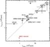 |
Fig. 7 CO(7–6) vs. the [CI]2–1 luminosity for a sample of high-z SMGs and QSO (grey circles) and the Spiderweb galaxy (red circles). The dotted curve is the 1–1 relation. |
4.1.3. Possible causes of observed line ratio
The Spiderweb galaxy is, like the Cloverleaf galaxy, an outlier, compared to lensed galaxies. This unusually low CO(7–6)/[CI]2–1 line ratio could be due to the Spiderweb galaxy being an extraordinary HzRG with a highly unusual ratio between the diffuse and dense molecular gas, or due to the impact of cosmic-ray heating and ionisation, or differential lensing.
Comparing  K km s-1 pc2 with
  K km s-1 pc2 (Emonts et al. 2013), we find that the CO(7–6) emission is only 18% of the value for thermalised gas. This indicates that the molecular gas phase is not thermalised and dominated by the cold and diffuse gas, which is traced by the [CI]2–1 emission line1. Alternatively, a fraction of the CO in the Spiderweb galaxy may be dissociated by cosmic-rays, increasing the fraction of atomic carbon in the molecular gas without strongly affecting the excitation of [CI]2–1 or the ionisation state of carbon (Bisbas et al. 2015). In the circum-nuclear region of a powerful radio galaxy, it is likely that cosmic rays may have had a significant impact on the nature of the molecular gas. More observations of other atomic and molecular species in the Spiderweb galaxy are necessary to investigate this quantitatively.
However, since the comparison sample are all lensed galaxies, the difference could also be caused by differential lensing in the comparison sample. Dense (traced by CO(7–6)) and diffuse (traced by [CI]2–1) gas in galaxies may be subject to differential lensing, where the emission from the densest gas has a higher overall magnification than the diffuse gas. Serjeant (2012) showed that for lensing magnifications μ> 2, the CO ladder can be strongly distorted by differential lensing. Since all the SMGs and QSOs listed in Table 3 have a magnification μ> 2, it may be that their line ratios are all influenced by the affect of differential lensing. If so, this implies that the CO(7–6) emission probably has a higher magnification than the [CI]2–1 emission, which would mean that the intrinsic CO(7–6)/[CI]2–1 ratio would be lower. We note, however, that although some of the data are limited by S/N and/or low resolution, the line profiles of CO(7–6) and [CI]2–1 are consistent with each other (see references listed in Table 3). While not conclusive, the similarity of their dynamics suggests that the gas probed by CO(7–6) and [CI]2–1 follow the same overall dynamics and are perhaps not strongly affected by differential lensing.
We are planning to extend our ALMA [CI] observations to eight HzRGs to verify if this low CO/[CI] ratio is a common feature and also carry out more detailed studies of the Spiderweb galaxy to investigate this puzzle.
4.2. Cooling of the post-shock gas owing to slow shocks in molecular halos
Interestingly, the two regions of H2O emission that we detect do not appear to be associated with significant dust continuum emission. This is puzzling since a close association between a dense gas tracer such as H2O and dust is expected when the excitation of the H2O emission in other high-z (lensed) sources has been attributed to IR pumping (van der Werf et al. 2011; Omont et al. 2013). Moreover, no H2O emission is detected at the position of the HzRG (Fig. 5), which is surprising, given its strong IR emission and high rate of mechanical energy injection via the radio jets (Fig. 5). Specifically, Omont et al. (2013) detect H2O for seven high-z lensed sources from the H-ATLAS survey. Five are detected in H2O 211−202 emission, and three in H2O 202−111 emission. Comparing these H2O detections to the 8–1000 μm IR luminosity, Omont et al. (2013) find a correlation between the IR and H2O line luminosity of  , with the exact exponent being dependent on which of the two H2O lines is used in the analysis. From this relation, they conclude that IR pumping is the most likely mechanism for exciting the water molecules and their line emission. This is consistent with H2O tracing dense gas that surrounds regions of intense star formation. Furthermore, a similar conclusion was reached in a more detailed study of the H2O emission from the lensed QSO, APM 08279+5255 at z = 3.9 (van der Werf et al. 2011) and by Yang et al. (2013), who detected H2O emission lines in 45 low-z galaxies.
Figure 8 plots LH2O/LIR versus LIR and shows an anti-correlation for IR luminous high-z lensed sources (Omont et al. 2013; van der Werf et al. 2011). SDP.81 is an outlier in this relation, most likely because of an underestimation of the H2O luminosity as a result of low S/N in the spectrum, and the large extent of the source (Omont et al. 2013). We plot the Spiderweb galaxy as the sum of the H2O luminosities of the western and eastern detections and the total infrared luminosity. The H2O emission originates from two small regions, and any more widespread emission would not be detected owing to the lack of sensitivity of our ALMA data on larger spatial scales. The IRAM Plateau de Bure observations of the comparison sample of Omont et al. (2013) have two to seven times larger synthesised beam sizes, and may be more sensitive to emission at larger scales. The LH2O/LFIR ratio for the Spiderweb galaxy is therefore a lower limit and the Spiderweb galaxy could therefore be an outlier in this trend. The lack of 246 GHz continuum emission at the H2O positions, which would imply a much larger deviation from the trend, implies that the emission is not pumped by the IR emission. The H2O detection is spatially located at the bend in the radio continuum emission (knot B3) and upstream to the radio jet. Similarly, the eastern H2O detection upstream from knot A in the radio emission is likely associated with the jet, which is projected onto the plane of the sky.
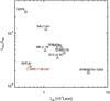 |
Fig. 8 LH2O/LIR-ratio versus intrinsic LIR for the H2O detections from Omont et al. (2013) along with the H2O detection for the Spiderweb galaxy. The grey circles are sources from Omont et al. (2013) with directed detections of the 202−111 line and the grey triangles are sources with 211−202 detection, scaled using Mrk231 as a template to get an estimate on the 202−111 luminosity. The Spiderweb galaxy is shown with the red point. We plot the summed H2O emission of the western and eastern detection, since the IR luminosity is integrated over the full source. |
The most straightforward explanation for the H2O emission at these positions, the lack of significant associated 246 GHz continuum emission, and the offset from the anti-correlation in Fig. 8, is that the H2O emitting gas is shock-heated and represents strong cooling in post-shock heated gas by the passage of the radio jet. H2O is one of the main carriers of oxygen along with CO, but has many more radiative degrees of freedom, meaning that it can lose energy efficiently under a wide range of (low energy) excitation conditions and thus contribute significantly to the overall cooling of dense molecular gas, in particular after the shock impact (Flower & Pineau Des Forêts 2010). Given the small offset of the line peaks from the systemic [CI]2–1 redshift, only 100 to 200 km s-1, and the average line width of 290 km s-1 of the two H2O lines, it is likely that the width of the lines represents the dispersion of the clouds and that mechanical energy is being dissipated within the dense molecular gas. Not only H2O, but also the detection of strong mid-infrared H2 emission (Ogle et al. 2012), suggest excitation of molecules in low-velocity shocks (see discussion in Guillard et al. 2009; Appleton et al. 2013). Moreover, we emphasise that, owing to the position of the H2O emission in our bandpass, higher negative offset velocity emission, such as that from companion #10, would not lie within our bandpass (Kuiper et al. 2011).
Furthermore, it is unlikely that the dense molecular gas has been entrained during the passage of the radio jet and lifted out of the radio galaxy or any of its companions. There are several reasons why this is unlikely. First, both regions of H2O emission are almost at the systemic velocity of the radio galaxy (as determined from CO(1–0), [CI]2–1 or CO(7–6)). The H2O lines have systemic velocities that are significantly lower than any of the companion galaxies with determined redshifts near the sites of H2O emission. Second, the cooling time of the dense shock gas is of-order 103−104 yr for a 20 km s-1 shock that was driven into a gas with a density of 105 cm-3 (Flower & Pineau Des Forêts 2010), which is much shorter than any plausible dynamical time. These facts suggest that the dense molecular gas is forming in situ in the post-shocked gas after the passage of the radio jet. Within this context, it is not surprising to see the emission near the bend in the jet and near the terminal hotspot of the western radio lobe since these are sites where the interaction between the jet and ambient medium are likely to be strong. In such strong interaction zones, dissipation of energy in a turbulent cascade is important (e.g. Guillard et al. 2010). The eastern terminal lobe of the jet is, for example, the working surface of the jet as it propagates outwards, which exactly the region where you would expect strong dissipation of the bulk kinetic energy of the jet.
The molecular gas likely formed in situ in the post-shock gas, which has important implications for the state of the circum-galactic halo and cluster gas. Recent observations of the Spiderweb galaxy using ATCA discovered a large region of CO(1–0) surrounding the HzRG with strong emission near some of the radio knots and lobes, which suggests that the passage of the radio jet enhances the molecular column densities (Emonts et al., in prep.). Finding strong H2O line emission near the radio jet provides evidence of the formation of molecular gas in the post-shocked gas of the expanding radio source (see Guillard et al. 2010, 2012; Appleton et al. 2013,for a discussion of this mechanism in the violent collision in the Stephan’s Quintet group). This is also substantiated by the low relative velocities of the H2O emission, which are consistent with the low velocities observed in the extended diffuse CO emission. Such a mechanism might also explain the distribution of the CO emission observed in local clusters (Salomé et al. 2011) and around other HzRGs (Emonts et al. 2014, and references therein). Finding H2O emission that indicates strong dissipation of the bulk kinetic energy of expanding radio jets provides a direct link between the jets and the formation of molecular gas and stars in the halo of the radio galaxy.
4.3. Mass estimates
As argued above, the [CI]2–1 line is a better tracer of the cold molecular gas than the high-J CO lines, owing to their lower critical density. We therefore use the [CI]2–1 to estimate the total molecular gas mass, following the approach of Papadopoulos et al. (2004) and Alaghband-Zadeh et al. (2013): ![Mathematical equation: \begin{eqnarray} \label{eq:Mh2} M_{\text{\Htwo}} &=& 1375.8\,D_{\rm L}^2\,(1+z)^{-1}\,{\left[\frac{X_{\text{[CI]}}}{10^{-5}}\right]}^{-1} \\ \nonumber &&\quad\times{\left[\frac{A_{21}}{10^{-7}\text{s}^{-1}}\right]}^{-1}Q_{21}^{-1} \left[\frac{S_{\text{[CI]2-1}}{\rm d}V}{\text{Jy\,km\,s}^{-1}}\right], \end{eqnarray}](/articles/aa/full_html/2016/07/aa27647-15/aa27647-15-eq168.png) (1)where X[ CI ] is the [CI]-to-H2 abundance for which we adopt the literature-standard of 3 × 10⁻⁵, Q21 is the density dependent excitation factor, for which we assume the median value of 0.57 (see Papadopoulos et al. 2004), and A21 is the Einstein A coefficient of 2.68 × 10⁻⁷ s-1. We find a total H2 molecular gas mass for both components of 3.3 × 10¹⁰ M⊙. We note that this value depends on the adopted Q21: for the highest Q21 = 1.0, the M(H2) drops to 2.2 × 10¹⁰ M⊙, while for the lowest Q21 = 0.15, the M(H2) is 1.5 × 10¹¹ M⊙ The median value is close to M(H2) = 6 × 10¹⁰ M⊙ that is derived from CO(1–0) (Emonts et al. 2013). This total mass of diffuse molecular gas, as probed by the [CI]2–1 emission, is clearly higher than the warm (T> 300 K) molecular gas mass of order 107 to 109 M⊙ (Ogle et al. 2012), which suggests an order of magnitude ratio of warm-to-cold molecular gas between 0.1−10%. Ogle et al. (2012) suggest that the gas is heated by the radio jet from the AGN interacting with the ambient ISM of the HzRG. Furthermore, Nesvadba et al. (2006) find a mass of ionised gas of ~3 × 10⁹ M⊙. The gas masses of various components of the ISM of the HzRG are up to one order of magnitude lower than the stellar mass of <1.8 × 10¹² M⊙ (De Breuck et al. 2010), suggesting that this is already quite an evolved galaxy.
(1)where X[ CI ] is the [CI]-to-H2 abundance for which we adopt the literature-standard of 3 × 10⁻⁵, Q21 is the density dependent excitation factor, for which we assume the median value of 0.57 (see Papadopoulos et al. 2004), and A21 is the Einstein A coefficient of 2.68 × 10⁻⁷ s-1. We find a total H2 molecular gas mass for both components of 3.3 × 10¹⁰ M⊙. We note that this value depends on the adopted Q21: for the highest Q21 = 1.0, the M(H2) drops to 2.2 × 10¹⁰ M⊙, while for the lowest Q21 = 0.15, the M(H2) is 1.5 × 10¹¹ M⊙ The median value is close to M(H2) = 6 × 10¹⁰ M⊙ that is derived from CO(1–0) (Emonts et al. 2013). This total mass of diffuse molecular gas, as probed by the [CI]2–1 emission, is clearly higher than the warm (T> 300 K) molecular gas mass of order 107 to 109 M⊙ (Ogle et al. 2012), which suggests an order of magnitude ratio of warm-to-cold molecular gas between 0.1−10%. Ogle et al. (2012) suggest that the gas is heated by the radio jet from the AGN interacting with the ambient ISM of the HzRG. Furthermore, Nesvadba et al. (2006) find a mass of ionised gas of ~3 × 10⁹ M⊙. The gas masses of various components of the ISM of the HzRG are up to one order of magnitude lower than the stellar mass of <1.8 × 10¹² M⊙ (De Breuck et al. 2010), suggesting that this is already quite an evolved galaxy.
For component 2, the H2 gas mass of the broad component is 1.6 × 10¹⁰ M⊙. We use this to constrain the size of this region by knowing that the molecular mass has to be smaller than the dynamical mass (M(H2) <Mdyn = R·v2/G), and by using the velocity from the FWHM (see Table 2), we find that R< 60 pc. Though uncertain, this region has a size comparable to those of the obscuring torus and the inner narrow line regions of QSOs, thus suggesting the presence of an additional radio-quiet AGN merging with the radio-loud AGN in component 1 (Emonts et al. 2015). Applying the same methods to component 1, which has a H2 gas mass of 1.7 × 10¹⁰, puts an upper limit of 1 kpc on the size of the emitting region.
To determine the dust mass, we need to integrate over the full SED of the dust emission. As we only have a single observation at 246 GHz, we fix the shape of the SED by assuming a greybody that is characterised by β = 1.5 and Td = 40 K. Following the approach of De Breuck et al. (2003), using  (2)where Sobs is the flux density at the observed frequency, DL is the luminosity distance, κd(νrest) is the rest-frequency mass absorption coefficient, which we here calculate by scaling the 850 μm absorption coefficient of 0.076 m2 kg-1 from Stevens et al. (2003) to 246 GHz, and B(νrest,Td) is the Planck function for isothermal dust grain emission at a dust temperature Td (De Breuck et al. 2003), we derive a dust mass of Md = 6.1 × 10⁸ M⊙ for the HzRG. This is marginally higher than what was estimated by Stevens et al. 2003 of 4.6 × 10⁸ M⊙ using the 850 μm flux peak flux.
Taking the same approach and assumed dust temperature, we find the dust masses of the two companions #8 and #10 (see Table 4).
4.4. Star formation rate
Using Spitzer and Herschel PACS+SPIRE photometry, Seymour et al. (2012) show that the strong AGN and vigorous star formation contribute with roughly equal amounts to the IR luminosity in the Spiderweb galaxy. While the AGN component dominates at the high frequency end of the thermal dust emission, the star formation is expected to contribute >90% of the flux at the observed (comparatively low) frequencies of our ALMA data. However, the flux spectral index of the HzRG and companion #10, implies that the flux at these wavelength are likely to be contaminated by synchrotron emission. We can therefore use our continuum flux to determine upper limits on the SFR in the host galaxy and the companions.
We estimate the SFR of the HzRG and companions by fixing the dust temperature and emissivity index (as for the dust masses) and calculating LFIR using  (3)which yields
 ![Mathematical equation: \begin{eqnarray} L_{\text{FIR}}=4 \pi \Gamma[\beta+4] \zeta [\beta+4] D_{\rm L}^2x^{-(\beta+4)}({\rm e}^x-1)S_{\text{obs}}\nu_{\text{obs}}, \end{eqnarray}](/articles/aa/full_html/2016/07/aa27647-15/aa27647-15-eq214.png) (4)where Γ and ζ are the Gamma and Riemann ζ functions and x = hνrest/kTd (De Breuck et al. 2003). Again, assuming β = 1.5 and Td = 40 K, we find the LFIR< 5.1 × 10¹² L⊙ for the HzRG, and <7.2 × 10¹¹ L⊙ for companion #8 and <5.4 × 10¹¹ L⊙ for companion #10 (see Table 4).
(4)where Γ and ζ are the Gamma and Riemann ζ functions and x = hνrest/kTd (De Breuck et al. 2003). Again, assuming β = 1.5 and Td = 40 K, we find the LFIR< 5.1 × 10¹² L⊙ for the HzRG, and <7.2 × 10¹¹ L⊙ for companion #8 and <5.4 × 10¹¹ L⊙ for companion #10 (see Table 4).
Using  (5)where δMF is the stellar mass function and δSB is the fraction of FIR emission that is heated by the starburst, which we assume to be unity at these long wavelengths, the LFIR can be converted to the SFR. We assume δMF = 1 and derive the SFRs of <440 M⊙ yr-1 for the HzRG, <62 M⊙ yr-1 for companion #8 and <47 M⊙ yr-1 for companion #10 (see Table 4). The sum of the estimated FIR luminosity of the HzRG and the two companion sources is higher than the total starburst-heated IR luminosity of 5.6 × 10¹²L⊙ of Drouart et al. 2014, less than the 7.9 × 10¹²L⊙ of Seymour et al. (2012). We warn that our approximation of the SED with a single greybody function with an assumed emissivity index is rather crude; moreover the 246 GHz emission from the HzRG and companion #10 may also contain a contribution from synchrotron emission, which would over-estimate the SFR.
4.4.1. SFR of the Spiderweb galaxy and its companions
Kuiper et al. (2011) find a bi-model velocity distribution of galaxies close in projection to the Spiderweb galaxy, which suggests two groups (or regions) of galaxies flowing into the circum-galactic environment at high velocity (~400 to 1600 km s-1). Comparing the velocity and spatial distribution of the galaxies with that found in massive halos at z ~ 2 within the Millennium simulation, they conclude that the Spiderweb galaxy is best described by the merger of two galaxy groups or flows of galaxies into the over-dense environment of the powerful HzRG.
The SFRs that we determine here for the HzRG and companion #10 and #8 are ~10–50 times higher than determined by Hatch et al. (2009) using optical HST imaging. However, the continuum emission in both the HzRG and companion #10 are contaminated by synchrotron emission. For the HzRG there are two components and only one of them, the AGN core, is contaminated up to ~50% (see Sect. 3.1). The fact that the continuum emission is extended in the direction that connects these two components (see Fig. 1) suggests that both must have roughly similar 246 GHz flux densities. The synchrotron contamination for the combined Spiderweb galaxy is therefore estimated to be no more than ~25%. For companion #10, all of the emission could be due to synchrotron (see Sect. 3.1). Observations of the synchrotron spectrum around ~100 GHz are needed to determine if it remains straight out to 246 GHz, or if there is a downturn owing to energy losses of the most energetic electrons. In the latter case, even companion #10 could still be dominated by star formation. In this extreme case, then its SFR and that of companion #8 would suggest that (over the scale of our ALMA data) about ~20% of the star formation is taking place outside the HzRG in companion sources. We note that companion #8 is a marginal 3σ detection and that the two additional companions (#12 and #17) show hints of 246 GHz emission at ~1.5σ significance. To confirm if these hints of emission are real requires deeper 246 GHz observations. For the remaining sources in the surroundings of the Spiderweb galaxy, the sensitivity of our data is too low to detect them, meaning that their SFR is ≲50 M⊙ yr-1.
5. Conclusions
We have observed the HzRG MRC1138-262 (the Spiderweb galaxy) with ALMA Band 6 in Cycle 1 for 49 min on-source.
-
We detect strong 246 GHz continuum emission at the position of the HzRG, weaker 246 GHz continuum emission for a companion to the west, and tentative emission to the north. Companion #10 of Kuiper et al. (2011) at z = 2.1446 is the brightest of the two companions and is detected in CO(7–6), while [CI]2–1 is shifted out of the observed band. The other companion is too weak to be detected in line emission.
-
The flat spectral indexes of the HzRG and companion #10 suggest a contribution to the 246 GHz continuum emission from synchrotron emission. This means that the FIR luminosities and SFRs of these two components are upper limits.
-
We detect strong [CI]2–1 emission in two components: one at the position of the HzRG, and one with a small offset of 0.̋5 to the south-east from the central position. The [CI]2–1 emitting components show significantly different velocity profiles: component 1 shows a Lorentzian profile, and component 2 is a double Gaussian with velocity widths of 250 and 1100 km s-1.
-
Using the molecular gas-mass estimate of the broad [CI]2–1 of component 2, we put an upper limit on the size of the emitting region of 60 pc. This size suggests the possible existence of an additional radio quiet AGN, merging with the radio loud AGN in component 1.
-
The CO(7–6)/[CI]2–1 line ratio for the Spiderweb galaxy is lower than that of a comparison sample. This ratio can be due to a relatively low excitation molecular gas reservoir and/or a strong cosmic ray field which, preferentially, destroys CO. As the comparison sample is composed of only lensed sources from the literature, differential lensing may also have an influence, where the dense CO(7–6) gas in the comparison sample is amplified more than the more diffuse [CI]2–1 gas.
-
We detect ~4σ H2O emission lines at two positions: to the west at knot B4 (at the bend) in the radio jet and to the east, upstream of knot A. No 246 GHz continuum emission is detected at the position of the H2O emission lines, meaning that heating from IR emission cannot be the source of the H2O emission. The positions (upstream of the two knots in the radio jet), the lack of 246 GHz continuum emission at these positions and the small offset of the line centres, are consistent with heating by slow shocks in dense molecular gas. The relatively bright H2O emission indicates strong dissipation of the energy of the expanding jets in the halo of MRC1138-262.
Multiple studies have established that the Spiderweb galaxy is a system of merging galaxies, and the likely progenitor of a cD galaxy. Our water detections upstream of the main radio hotspots show that the radio jets can cause the gas in the ISM and inter-cluster gas to cool, increasing the fraction of extended molecular gas (Emonts et al., in prep.). The formation of this molecular reservoir likely supports the formation of the young stars that are observed in the halo of MRC1138-262. The much brighter than expected [CI]2–1 emission indicates the power of this line to study the detailed distribution of the molecular gas reservoir in this intriguing source, and possibly other HzRGs.
Note, however, that the high spatial resolution of the ALMA observation means that up to 2/3 of the CO(7–6) emission may not be detected owing to lack of sensitivity to very extended, low surface-brightness line emission (Emonts et al., in prep.).
Acknowledgments
This paper makes use of the following ALMA data: ADS/JAO.ALMA#2012.1.01087.S. ALMA is a partnership of ESO (representing its member states), NSF (USA) and NINS (Japan), together with NRC (Canada), NSC and ASIAA (Taiwan), and KASI (Republic of Korea), in cooperation with the Republic of Chile. The Joint ALMA Observatory is operated by ESO, AUI/NRAO, and NAOJ. B.G. acknowledges support from the ERC Advanced Investigator programme DUSTYGAL 321334. B.E. acknowledges funding through the European Union FP7-PEOPLE-2013-IEF grand 62435.
References
- Alaghband-Zadeh, S., Chapman, S. C., Swinbank, A. M., et al. 2013, MNRAS, 435, 1493 [Google Scholar]
- Alloin, D., Guilloteau, S., Barvainis, R., Antonucci, R., & Tacconi, L. 1997, A&A, 321, 24 [NASA ADS] [Google Scholar]
- Appleton, P. N., Guillard, P., Boulanger, F., et al. 2013, ApJ, 777, 66 [NASA ADS] [CrossRef] [Google Scholar]
- Bicknell, G. V., Dopita, M. A., Tsvetanov, Z. I., & Sutherland, R. S. 1998, ApJ, 495, 680 [NASA ADS] [CrossRef] [Google Scholar]
- Bisbas, T. G., Papadopoulos, P. P., & Viti, S. 2015, ApJ, 803, 37 [NASA ADS] [CrossRef] [Google Scholar]
- Carilli, C. L., Röttgering, H. J. A., van Ojik, R., et al. 1997, ApJS, 109, 1 [NASA ADS] [CrossRef] [Google Scholar]
- Carilli, C. L., Harris, D. E., Pentericci, L., et al. 2002, ApJ, 567, 781 [NASA ADS] [CrossRef] [Google Scholar]
- Cox, P., Krips, M., Neri, R., et al. 2011, ApJ, 740, 63 [NASA ADS] [CrossRef] [Google Scholar]
- Danielson, A. L. R., Swinbank, A. M., Smail, I., et al. 2011, MNRAS, 410, 1687 [NASA ADS] [Google Scholar]
- Dannerbauer, H., Kurk, J. D., De Breuck, C., et al. 2014, A&A, 570, A55 [NASA ADS] [CrossRef] [EDP Sciences] [Google Scholar]
- De Breuck, C., Neri, R., Morganti, R., et al. 2003, A&A, 401, 911 [NASA ADS] [CrossRef] [EDP Sciences] [Google Scholar]
- De Breuck, C., Seymour, N., Stern, D., et al. 2010, ApJ, 725, 36 [NASA ADS] [CrossRef] [Google Scholar]
- Downes, D., & Solomon, P. M. 2003, ApJ, 582, 37 [NASA ADS] [CrossRef] [Google Scholar]
- Drouart, G., De Breuck, C., Vernet, J., et al. 2014, A&A, 566, A53 [NASA ADS] [CrossRef] [EDP Sciences] [Google Scholar]
- Emonts, B. H. C., Feain, I., Röttgering, H. J. A., et al. 2013, MNRAS, 430, 3465 [NASA ADS] [CrossRef] [Google Scholar]
- Emonts, B. H. C., Norris, R. P., Feain, I., et al. 2014, MNRAS, 438, 2898 [NASA ADS] [CrossRef] [Google Scholar]
- Emonts, B. H. C., De Breuck, C., Lehnert, M. D., et al. 2015, A&A, 584, A99 [NASA ADS] [CrossRef] [EDP Sciences] [Google Scholar]
- Ferkinhoff, C., Brisbin, D., Parshley, S., et al. 2014, ApJ, 780, 142 [NASA ADS] [CrossRef] [Google Scholar]
- Flower, D. R., & Pineau Des Forêts, G. 2010, MNRAS, 406, 1745 [NASA ADS] [Google Scholar]
- Glover, S. C. O., Clark, P. C., Micic, M., & Molina, F. 2015, MNRAS, 448, 1607 [NASA ADS] [CrossRef] [Google Scholar]
- Goicoechea, J. R., Chavarría, L., Cernicharo, J., et al. 2015, ApJ, 799, 102 [NASA ADS] [CrossRef] [Google Scholar]
- Greve, T. R., Ivison, R. J., & Stevens, J. A. 2006, Astron. Nachr., 327, 208 [NASA ADS] [CrossRef] [Google Scholar]
- Guillard, P., Boulanger, F., Pineau Des Forêts, G., & Appleton, P. N. 2009, A&A, 502, 515 [NASA ADS] [CrossRef] [EDP Sciences] [Google Scholar]
- Guillard, P., Boulanger, F., Cluver, M. E., et al. 2010, A&A, 518, A59 [NASA ADS] [CrossRef] [EDP Sciences] [Google Scholar]
- Guillard, P., Boulanger, F., Pineau des Forêts, G., et al. 2012, ApJ, 749, 158 [NASA ADS] [CrossRef] [Google Scholar]
- Hatch, N. A., Overzier, R. A., Röttgering, H. J. A., Kurk, J. D., & Miley, G. K. 2008, MNRAS, 383, 931 [NASA ADS] [CrossRef] [Google Scholar]
- Hatch, N. A., Overzier, R. A., Kurk, J. D., et al. 2009, MNRAS, 395, 114 [NASA ADS] [CrossRef] [Google Scholar]
- Humphrey, A., Villar-Martín, M., Vernet, J., et al. 2008, MNRAS, 383, 11 [NASA ADS] [CrossRef] [Google Scholar]
- Kneib, J.-P., Neri, R., Smail, I., et al. 2005, A&A, 434, 819 [NASA ADS] [CrossRef] [EDP Sciences] [Google Scholar]
- Kuiper, E., Hatch, N. A., Miley, G. K., et al. 2011, MNRAS, 415, 2245 [NASA ADS] [CrossRef] [Google Scholar]
- Kurk, J. D., Pentericci, L., Overzier, R. A., Röttgering, H. J. A., & Miley, G. K. 2004a, A&A, 428, 817 [NASA ADS] [CrossRef] [EDP Sciences] [Google Scholar]
- Kurk, J. D., Pentericci, L., Röttgering, H. J. A., & Miley, G. K. 2004b, A&A, 428, 793 [NASA ADS] [CrossRef] [EDP Sciences] [Google Scholar]
- Lestrade, J.-F., Combes, F., Salomé, P., et al. 2010, A&A, 522, L4 [NASA ADS] [CrossRef] [EDP Sciences] [Google Scholar]
- Lonsdale, C. J., & Barthel, P. D. 1986, AJ, 92, 12 [NASA ADS] [CrossRef] [Google Scholar]
- Lupu, R. E., Scott, K. S., Aguirre, J. E., et al. 2012, ApJ, 757, 135 [NASA ADS] [CrossRef] [Google Scholar]
- Miley, G. K., Overzier, R. A., Zirm, A. W., et al. 2006, ApJ, 650, L29 [NASA ADS] [CrossRef] [Google Scholar]
- Nesvadba, N. P. H., Lehnert, M. D., Eisenhauer, F., et al. 2006, ApJ, 650, 693 [NASA ADS] [CrossRef] [Google Scholar]
- Ogle, P., Davies, J. E., Appleton, P. N., et al. 2012, ApJ, 751, 13 [NASA ADS] [CrossRef] [Google Scholar]
- Omont, A., Yang, C., Cox, P., et al. 2013, A&A, 551, A115 [NASA ADS] [CrossRef] [EDP Sciences] [Google Scholar]
- Papadopoulos, P. P., Thi, W.-F., & Viti, S. 2004, MNRAS, 351, 147 [NASA ADS] [CrossRef] [Google Scholar]
- Pentericci, L., Röttgering, H. J. A., Miley, G. K., Carilli, C. L., & McCarthy, P. 1997, A&A, 326, 580 [NASA ADS] [Google Scholar]
- Pentericci, L., Röttgering, H. J. A., Miley, G. K., et al. 1998, ApJ, 504, 139 [NASA ADS] [CrossRef] [Google Scholar]
- Pentericci, L., Kurk, J. D., Röttgering, H. J. A., et al. 2000, A&A, 361, L25 [NASA ADS] [Google Scholar]
- Pentericci, L., Kurk, J. D., Carilli, C. L., et al. 2002, A&A, 396, 109 [NASA ADS] [CrossRef] [EDP Sciences] [Google Scholar]
- Riechers, D. A., Bradford, C. M., Clements, D. L., et al. 2013, Nature, 496, 329 [Google Scholar]
- Röttgering, H. J. A., van Ojik, R., Miley, G. K., et al. 1997, A&A, 326, 505 [NASA ADS] [Google Scholar]
- Salomé, P., Combes, F., Revaz, Y., et al. 2011, A&A, 531, A85 [NASA ADS] [CrossRef] [EDP Sciences] [Google Scholar]
- Serjeant, S. 2012, MNRAS, 424, 2429 [NASA ADS] [CrossRef] [Google Scholar]
- Seymour, N., Altieri, B., De Breuck, C., et al. 2012, ApJ, 755, 146 [NASA ADS] [CrossRef] [Google Scholar]
- Stevens, J. A., Ivison, R. J., Dunlop, J. S., et al. 2003, Nature, 425, 264 [NASA ADS] [CrossRef] [PubMed] [Google Scholar]
- van der Werf, P. P., Berciano Alba, A., Spaans, M., et al. 2011, ApJ, 741, L38 [NASA ADS] [CrossRef] [Google Scholar]
- Walter, F., Weiß, A., Downes, D., Decarli, R., & Henkel, C. 2011, ApJ, 730, 18 [NASA ADS] [CrossRef] [Google Scholar]
- Weiß, A., Henkel, C., Downes, D., & Walter, F. 2003, A&A, 409, L41 [NASA ADS] [CrossRef] [EDP Sciences] [Google Scholar]
- Yang, C., Gao, Y., Omont, A., et al. 2013, ApJ, 771, L24 [NASA ADS] [CrossRef] [Google Scholar]
All Tables
H2O, [CI]2–1 and CO(7–6) emission line positions, velocity integrated fluxes, and FWHMs.
SMGs and QSOs from the literature with published [CI]2–1, CO(7–6) and H2O detections along with published IR luminosities used for comparison to the Spiderweb galaxy.
All Figures
|
Fig. 1 Overview of the spatial distribution of the detected components. The naturally weighted 246 GHz continuum map is in greyscale and the two [CI]2–1 components, 1 and 2, are shown with blue and red ellipses, respectively. The two H2O detections are shown with orange ellipses, and the 246 GHz continuum components shown with green ellipses. The sizes of the ellipses represent the extractions used for the photometry. The knots in the radio jet are indicated with red-orange diamonds and labeled according to Pentericci et al. (1997). The numbers correspond to the numbering in Kuiper et al. (2011). The ALMA beam is shown as a black ellipse in the lower left corner. |
| In the text | |
|
Fig. 2 Bottom panel: HST F814W image (Hatch et al. 2008) in greyscale overlaid with the naturally weighted 246 GHz continuum map in green contours with levels of 1.5σ, 3σ, and 5σ. In the naturally weighted continuum map, we detect emission from companion #10 (and tentatively from #8) of Kuiper et al. (2011). The purple cross indicate the position of the nearby Ly α emitter at the position of the HzRG. The purple circles indicate the positions of Ly α emitters, the squares show the position of Hα and the triangles extremely red objects within the Ly α halo of MRC1138-262. The Ly α emitter #491 is offset by 0.̋8 from the companion source seen in the 246 GHz continuum emission west of the HzRG. Top panel: zoom in of the region around the companion sources. The purple circle shows the position of the Hα emitter #491 (Kurk et al. 2004b), which is close to the companion source seen in dust continuum emission. |
| In the text | |
|
Fig. 3 [CI]2–1 spectra and moment-0 maps for component 1, component 2, and the total [CI]2–1 and CO(7–6) emission. Top row: the spectra extracted from beam-sized areas for component 1, component 2, and the total. The areas from which the spectra of component 1 and component 2 are extracted do not overlap. The Lorentzian profile for the component 1 [CI]2–1 line (top left), the double Gaussian profile for the component 2 [CI]2–1 line (top middle), and the single Gaussian fits for the two CO(7–6) lines are over-plotted as black curves. The sum of the Lorentzian and Gaussian profiles is over-plotted in black in the total spectrum (top right). The dashed lines indicate the 0-velocity of the [CI]2–1 frequency at z = 2.1606, and the dotted lines indicate the 0-velocity for the CO(7–6) frequency at the same redshift. This redshift is in agreement with the redshift determined from the CO(1–0) line (Emonts et al. 2013). The dotted-dashed line indicate the 0-velocity of the [CI]2–1 frequency at z = 2.156, determined from the HeII λ1640Å line (which, as a non-resonant line, should represent the systemic velocity of the AGN, Humphrey et al. 2008). Bottom row: the moment-0 maps of the [CI]2–1 emission from component 1 (bottom left), component 2 (bottom middle), and the total (bottom right) [CI]2–1 emission and zoom-ins of the centres of the images. The total [CI]2–1 moment-0 maps is overlaid with [CI]2–1 line contours of component 1and 2. The blue and red crosses indicate the peaks of the [CI]2–1 emission of component 1 (blue) and component 2 (red). |
| In the text | |
|
Fig. 4 Bottom panel: moment-0 map of the CO(7–6) emission at the position of the brightest companion. Top panel: spectrum extracted from the beam-size area shown by the blue ellipse at the position of the companion sources in the bottom panel and is binned to 30 km s-1 channels. The spectrum shows both the continuum and CO(7–6) line emission. The redshift of the line is consistent with the optical z = 2.1446 (Kuiper et al. 2011), which was taken as zero velocity in the spectrum. |
| In the text | |
|
Fig. 5 Non-continuum subtracted H2O spectra for the detection of the west and east and the non-detection at the position at the HzRG and H2O moment-0 map. Top left panel: H2O line detected ~50 kpc to the east of the radio core, has a 3.7σ significance. The emission is located due west of the knot A in the radio jet. The fitted Gaussian is over-plotted in orange. Top middle panel: spectrum at the position of the radio core, shows no detection of H2O emission – only continuum emission. A small separation between the two spectral windows results in the gap in the continuum between − 1300 and − 1500 km s-1. Top right panel: H2O line detected ~25 kpc to the west of the radio core, showing a 4σ H2O detection at the expected frequency for z = 2.161. The emission is located at the bend of the radio jet, B4 (Pentericci et al. 1997). The best-fit Gaussian is over-plotted in orange. Bottom panel: moment-0 map of the H2O emission (without continuum subtraction), overlaid with the 246 GHz continuum emission in green contours. The orange ellipses show the H2O emission and the orange-red diamonds the positions of the knots in the radio jet, given by Pentericci et al. (1997). |
| In the text | |
|
Fig. 6 [CI]2–1 spectra (dark blue, dark red and black histograms) for component 1, component 2, and the total over-plotted with the respective CO(7–6) lines (light blue, orange and white histograms) to compare the velocity profiles. The fitted profiles from Sect. 3 are over-plotted as black curves, with the individual velocity components as dotted lines. The narrow [CI]2–1 component of component 2 is offset by 365 km s-1 from the systemic redshift. The bar above the velocity profiles in the right plot, marked the HeII redshift and errors (olive bar) from Röttgering et al. (1997) and the CO(1–0) redshift and error (blue bar) from Emonts et al. (2013). |
| In the text | |
|
Fig. 7 CO(7–6) vs. the [CI]2–1 luminosity for a sample of high-z SMGs and QSO (grey circles) and the Spiderweb galaxy (red circles). The dotted curve is the 1–1 relation. |
| In the text | |
|
Fig. 8 LH2O/LIR-ratio versus intrinsic LIR for the H2O detections from Omont et al. (2013) along with the H2O detection for the Spiderweb galaxy. The grey circles are sources from Omont et al. (2013) with directed detections of the 202−111 line and the grey triangles are sources with 211−202 detection, scaled using Mrk231 as a template to get an estimate on the 202−111 luminosity. The Spiderweb galaxy is shown with the red point. We plot the summed H2O emission of the western and eastern detection, since the IR luminosity is integrated over the full source. |
| In the text | |
Current usage metrics show cumulative count of Article Views (full-text article views including HTML views, PDF and ePub downloads, according to the available data) and Abstracts Views on Vision4Press platform.
Data correspond to usage on the plateform after 2015. The current usage metrics is available 48-96 hours after online publication and is updated daily on week days.
Initial download of the metrics may take a while.