| Issue |
A&A
Volume 588, April 2016
|
|
|---|---|---|
| Article Number | A28 | |
| Number of page(s) | 15 | |
| Section | Stellar structure and evolution | |
| DOI | https://doi.org/10.1051/0004-6361/201527832 | |
| Published online | 14 March 2016 | |
Simulating the environment around planet-hosting stars
I. Coronal structure
1 European Southern Observatory, Karl-Schwarzschild-Str. 2, 85748 Garching bei München, Germany
e-mail: This email address is being protected from spambots. You need JavaScript enabled to view it.
2 Universitäts-Sternwarte München, Ludwig-Maximilians-Universität, Scheinerstr. 1, 81679 München, Germany
3 Institut de Recherche en Astrophysique et Planétologie, Université de Toulouse, UPS-OMP, 31400 Toulouse, France
4 Harvard-Smithsonian Center for Astrophysics, 60 Garden Street, Cambridge, MA 02138, USA
5 Center for Space Environment Modeling, University of Michigan, 2455 Hayward St., Ann Arbor, MI 48109, USA
Received: 25 November 2015
Accepted: 17 January 2016
Abstract
We present the results of a detailed numerical simulation of the circumstellar environment around three exoplanet-hosting stars. A modern global magnetohydrodynamic model is considered that includes Alfvén wave dissipation as a self-consistent coronal heating mechanism. This paper contains the description of the numerical set-up, evaluation procedure, and the simulated coronal structure of each system (HD 1237, HD 22049, and HD 147513). The simulations are driven by surface magnetic field maps, recovered with the observational technique of Zeeman-Doppler imaging. A detailed comparison of the simulations is performed, where two different implementations of this mapping routine are used to generate the surface field distributions. Quantitative and qualitative descriptions of the coronae of these systems are presented, including synthetic high-energy emission maps in the extreme ultraviolet (EUV) and soft X-ray (SXR) ranges. Using the simulation results, we are able to recover similar trends as in previous observational studies, including the relation between the magnetic flux and the coronal X-ray emission. Furthermore, for HD 1237 we estimate the rotational modulation of the high-energy emission that is due to the various coronal features developed in the simulation. We obtain variations during a single stellar rotation cycle of up to 15% for the EUV and SXR ranges. The results presented here will be used in a follow-up paper to self-consistently simulate the stellar winds and inner astrospheres of these systems.
Key words: stars: coronae / stars: magnetic field / stars: late-type / stars: individual: HD 1237 / stars: individual: HD 22049 / stars: individual: HD 147513
© ESO, 2016
1. Introduction
Analogous to the 11-year solar activity cycle, a large portion of late-type stars (~60%) show chromospheric activity cycles, with periods ranging from 2.5 to 25 years (Baliunas et al. 1995). For a very limited number of these systems, including binaries, the coronal X-ray counterparts of these activity cycles have also been identified (e.g. Favata et al. 2008; Robrade et al. 2012). These periodic signatures appear as a result of the magnetic cycle of the star. In the case of the Sun, this is completed every 22 years, during which the polarity of the large-scale magnetic field is reversed twice (Hathaway 2010). These elements, the cyclic properties of the activity and magnetic field, constitute a major benchmark for any dynamo mechanism proposed for the magnetic field generation (Charbonneau 2014).
Planet-hosting systems and their observational properties.
Recent developments in instrumentation and observational techniques have opened a new window for stellar magnetic field studies across the HR diagram (see Donati & Landstreet 2009). In particular, the large-scale surface magnetic field topology in stars different from the Sun can be retrieved using the technique of Zeeman-Doppler imaging (ZDI, Semel 1989; Brown et al. 1991; Donati & Brown 1997; Piskunov & Kochukhov 2002; Hussain et al. 2009; Kochukhov & Wade 2010). Several studies have shown the robustness of this procedure, successfully recovering the field distribution on the surfaces of Sun-like stars, over a wide range of activity levels (e.g. Donati et al. 2008; Petit et al. 2008; Alvarado-Gómez et al. 2015; Hussain et al. 2016). Long-term ZDI monitoring of particular Sun-like targets have shown different time-scales of variability in the large-scale magnetic field. This includes fast and complex evolution without polarity reversals (e.g. HN Peg, Boro Saikia et al. 2015), erratic polarity changes (e.g. ξ Boo, Morgenthaler et al. 2012), and hints of magnetic cycles with single (e.g. HD 190771, Petit et al. 2009) and double (e.g. τ Boo, Fares et al. 2009) polarity reversals on a time-scale of 1−2 years.
Furthermore, ZDI maps have proven to be very useful in other aspects of cool stellar systems research. Applications cover magnetic activity modelling for radial velocity jitter corrections (Donati et al. 2014), transit variability and bow-shocks (Llama et al. 2013), coronal X-ray emission (Johnstone et al. 2010; Arzoumanian et al. 2011; Lang et al. 2014), and mass-loss rates in connection with stellar winds (Cohen et al. 2010; Vidotto et al. 2011).
In the case of planet-hosting systems, ZDI-based studies have tended to focus on close-in exoplanet environments by applying detailed global three-dimensional magnetohydrodynamic (MHD) models that were originally developed for the solar system (BATS-R-US code, Powell et al. 1999). This numerical treatment includes all the relevant physics for calculating a stellar corona and wind model, using the surface magnetic field maps as driver of a steady-state solution for each system. Within the MHD regime, two main approaches have been considered: an ad hoc thermally driven polytropic stellar wind (i.e. P ∝ ργ, with γ as the polytropic index, Cohen et al. 2011; Vidotto et al. 2012, 2015), and a more recent description, with Alfvén wave turbulence dissipation as a self-consistent driver of the coronal heating and the stellar wind acceleration in the model (Cohen et al. 2014). This last scheme is based on the strong observational evidence that Alfvén waves that are of sufficient strength to drive the solar wind permeate the solar chromosphere (De Pontieu et al. 2007; McIntosh et al. 2011). Additionally, this numerical approach has been extensively validated against STEREO/EUVI and SDO/AIA measurements (see van der Holst et al. 2014). The models presented in this paper are based on this latest treatment of the heating and energy transfer in the corona.
In this work we present the results of a detailed numerical simulation of the circumstellar environment around three late-type exoplanet-hosts (HD 1237, HD 22049 and HD 147513), using a 3D MHD model. This first article contains the results of the simulated coronal structure, while the wind and inner astrosphere domains will be presented in a follow-up paper. The simulations are driven by the radial component of the large-scale surface magnetic field in these stars, which have been recovered using two different implementations of ZDI (Sect. 2). All three systems have similar coronal (X-ray) activity levels (see Table 1). While these are more active than the Sun, they would be classified as moderately active stars and well below the X-ray/ activity saturation level. A description of the numerical set-up is provided in Sect. 3, and the results are presented in Sect. 4. Section 5 contains a discussion in the context of other studies, and the conclusions of our work are summarized in Sect. 6.
2. Large-scale magnetic field maps
HD 1237, HD 147513, and HD 22049 are cool main-sequence stars (G8, G5, and K2, respectively) with relatively slow rotation rates (Prot ~ 7−12 days). Each of these systems hosts a Jupiter-mass planet (Mpsini>M♃), with orbital separations similar to the solar system planets (Hatzes et al. 2000; Naef et al. 2001; Mayor et al. 2004; Benedict et al. 2006). Table 1 contains a summary of the relevant astrophysical parameters for each system, taken from various observational studies.
Previous works have recovered the large-scale magnetic field on the surfaces of these stars by applying ZDI to time-series of circularly polarised spectra (Jeffers et al. 2014; Alvarado-Gómez et al. 2015; Hussain et al. 2016). For the stars included in this work, this has been done with the spectropolarimeter NARVAL at the Telescope Bernard Lyot (Aurière 2003), and the polarimetric mode (Piskunov et al. 2011) of the HARPS echelle spectrograph (Mayor et al. 2003) on the ESO 3.6 m telescope at La Silla Observatory. For consistency, the ZDI maps used in the simulations have been reconstructed using data from the same instrument1 (i.e. HARPSpol).
For the magnetic field mapping procedure, we considered two different approaches; the classic ZDI reconstruction, in which each component of the magnetic field vector is decomposed into a series of independent magnetic-image pixels (Brown et al. 1991; Donati & Brown 1997), and the spherical harmonics decomposition (SH-ZDI), where the field is described by the sum of a potential and a toroidal component and each component is expanded in a spherical-harmonics basis (see Hussain et al. 2001; Donati et al. 2006). Both procedures are equivalent, leading to very similar field distributions and associated fits to the spectro-polarimetric data. However, as described by Brown et al. (1991), ZDI is not able to properly recover very simple field geometries (e.g. dipoles) and is more suitable for complex (spotted) magnetic distributions. This limitation is removed in the SH-ZDI implementation. Both procedures are restricted by the inclination angle of the star, and therefore a fraction of the surface field that cannot be observed is not recovered in the maps. To correct for this effect, previous numerical studies have completed the field distribution by a reflection of the ZDI map across the equatorial plane (e.g. Cohen et al. 2010). More recently, Vidotto et al. (2012) have included complete symmetric and antisymmetric SH-ZDI maps to show that the map incompleteness has a minor effect on their simulation results. However, for the simulations performed here, which include the latest implementation of BATS-R-US, this may not be the case. A larger effect may be expected on the overall coronal structure, as the mechanism for the coronal heating and the wind acceleration is directly related to the field strength and topology (e.g. Alfvén waves, see van der Holst et al. 2014).
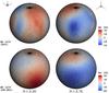 |
Fig. 1 Surface radial magnetic field maps of HD 1237. A comparison between the standard ZDI (top) and the SH-ZDI (bottom) is presented. The colour scale indicates the polarity and the field strength in Gauss (G). Note the difference in the magnetic field range for each case. The stellar inclination angle (i = 50°) is used for the visualisations. |
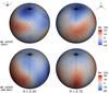 |
Fig. 2 Surface radial magnetic field maps of HD 22049. See caption of Fig. 1. The stellar inclination angle (i = 45°) is used for the visualisations. |
Figures 1 and 2 show a comparison between the reconstruction procedures applied to HD 1237 and HD 22049, respectively. In general, the maps obtained using ZDI show a more complex and weaker field distribution than the SH-ZDI, where a smoother field topology is obtained. While there are similarities in the large-scale structure, discrepancies are obtained in terms of the amount of detail recovered in each case. These differences arise as a consequence of the constraints imposed for completing the SH-ZDI maps, which are all pushed to symmetric field distributions. In general, the spatial resolution of the SH-ZDI maps depends on the maximum order of the spherical harmonics expansion (lmax). For each case this is selected in such a way that the lowest possible lmax value is used, while achieving a similar goodness-of-fit level (reduced χ2) as the classic ZDI reconstruction (HD 1237: lmax = 5, HD 22049: lmax = 6, HD 147513: lmax = 4). Higher values of lmax would not alter the large-scale distribution, but would introduce additional small-scale field without significantly improving the goodness-of-fit. This step is particularly important for a consistent comparison because the final recovered field strengths depend on this. All these differences affect the coronal and wind structure because they depend on the field coverage and the amount of magnetic energy available in each case (see Table 1). The standard ZDI reconstruction was not possible for HD 147513 because of its low inclination angle (i ~ 20°) and fairly simple large-scale topology. Therefore, we only considered the SH-ZDI map presented in Fig. 3 for this system, which was previously published by Hussain et al. (2016).
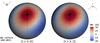 |
Fig. 3 Surface radial magnetic field maps of HD 147513 using SH-ZDI. Two rotational phases (Φ) are presented. The stellar inclination angle (i = 20°) is used for the visualisations. |
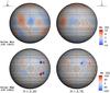 |
Fig. 4 Surface radial magnetic field maps of the Sun during activity minimum (CR 1922, top) and maximum (CR 1962, bottom) taken by SOHO/MDI. Note the difference in the magnetic field range for each case. An inclination angle i = 90° is used for the visualisations. |
To evaluate our numerical results, we performed two additional simulations taking the Sun as reference. The magnetic field distributions during solar minimum (Carrington rotation 1922, end of cycle 22), and solar maximum (Carrington rotation 1962, during cycle 23) were considered for this purpose. The large-scale magnetic field was taken from synoptic magnetograms, generated by the Michelson Doppler Imager instrument (MDI, Scherrer et al. 1995) on board the Solar and Heliospheric Observatory spacecraft (SOHO, Domingo et al. 1995). Figure 4 shows the comparison between the global magnetic field distribution for these activity epochs. During activity minimum, weak magnetic regions (a few Gauss) tend to be sparsely distributed across the entire solar surface (no preferential location for these regions is observed). Stronger small-scale magnetic fields, up to two orders of magnitude, can be found during activity maximum. In this case the dominant fields are highly concentrated in bipolar sectors (active regions) and are located mainly in two latitudinal belts at ~± 30°. Still, weaker magnetic fields can be found along the entire solar surface.
Finally, as is shown in Figs. 1 to 4, the numerical grid for all the input surface magnetic field distributions is the same. Therefore, the resolution of the solar coronal models was adapted to match the optimal resolution of the stellar simulations. In this way, a more consistent comparison of the results can be performed. The surface grid resolution (~10-2R∗) is sufficient to resolve the magnetic structures on the stellar ZDI/SH-ZDI maps entirely. However, in the solar case the internal structure of the active regions and the small-scale structures are not resolved. The effect of this limited resolution in magnetic field maps for solar simulations has been investigated previously by Garraffo et al. (2013). They found that the structure of the stellar wind is less sensitive to this factor than the coronal structure and associated emission (e.g. EUV and X-rays). This will be explored in more detail in the evaluation procedure, presented in Sect. 4.1.
3. 3D MHD numerical simulation
The numerical simulations presented here were performed using the 3D MHD code BATS-R-US (Powell et al. 1999) as part of the Space Weather Modeling Framework (SWMF, Tóth et al. 2012). As discussed previously by Cohen et al. (2014), the SWMF encompasses a collection of physics-based models for different regimes in solar and space physics. These can be considered individually or can be coupled together to provide a more realistic description of the phenomenon or domain of interest. For the systems considered here, we included and coupled two overlapping domains to obtain a robust combined solution. The results we present here correspond to the stellar corona domain (SC module). A follow-up study will describe the wind and the inner astrosphere (IH module). The solution for each domain was obtained using the most recent version of the SWMF modules2.
The stellar corona domain extends from the base of the chromosphere (~1 R∗) up to 30 R∗. A 3D potential field extrapolation above the stellar surface was used as the initial condition. This initial extrapolation was performed based on the photospheric radial magnetic field of the star (e.g. ZDI maps, Sect. 2). In addition to the surface magnetic field distribution, this module requires information about the chromospheric base density, n0, and temperature, T0, as well as the stellar mass, M∗, radius, R∗ and rotation period, Prot. This differs from previous ZDI-driven numerical studies, where these thermodynamic boundary conditions were set to coronal values and were therefore not obtained self-consistently in the simulations (Cohen et al. 2011; Vidotto et al. 2012, 2015).
For the stars considered here, we assumed solar values for the chromospheric base density (n0 = 2.0 × 10¹⁶ m-3), and temperature (T0 = 5.0 × 10⁴ K). This is justified because these systems, while more active than the Sun, are still within the X-ray un-saturated regime and the physical assumptions behind the coronal structure and the solar wind acceleration in the model are therefore more likely to hold. This assumption permits a consistent comparison with the solar case and between the systems considered. The remaining initial required parameters for each star are listed in Table 1. For the solar runs we used the sidereal rotation rate of 25.38 days (Carrington rotation).
We used a non-uniform spherical grid, dynamically refined at the locations of magnetic field inversion, which provides a maximum resolution of ~10-3R∗. The numerical simulation evolves until a steady-state solution is achieved. Coronal heating and stellar wind acceleration due to Alfvén wave turbulence dissipation were calculated self-consistently and took electron heat conduction and radiative cooling effects into account. For more details we refer to Sokolov et al. (2013) and van der Holst et al. (2014). From this final solution, all the physical properties, such as number density, n, plasma temperature, T, velocity, u and magnetic field, B, can be extracted. We present the simulation results in the following section.
4. Results
We performed a detailed evaluation of the solution sets for the solar minimum and maximum cases in Sect. 4.1. Sections 4.2 to 4.4 contain the simulation results of the coronal structure for the stars considered. In each case we present the distribution of the thermodynamic conditions (n, T) and the magnetic energy density (εB r), which is associated with the radial field. A common colour scale is adopted for all stars to facilitate comparison3.
In addition, synthetic coronal emission maps were generated at soft X-ray (SXR) and extreme ultraviolet (EUV) wavelengths. This was done by integrating the square of the plasma density times the emissivity response function of a particular instrument along the line of sight towards the observer. In the SXR range we considered the specific response function of the AlMg filter of the SXT/Yohkoh instrument to synthesise images in the 2 to 30 Å range (0.25−4.0 keV, red images). For the EUV range we used the sensitivity tables of the EIT/SOHO instrument, which led to narrow-band images centred at the Fe IX/X 171 Å (blue), Fe XII 195 Å (green), and Fe XV 284 Å (yellow) lines. The coronal emission at these wavelengths has been extensively studied in the solar context and also served to calibrate the results from the SWMF in various works (see Garraffo et al. 2013; van der Holst et al. 2014). This procedure also allows the direct comparison of the synthetic images that are generated for different stars. For HD 1237 and HD 22049 we additionally compared the results driven by the different maps of the large-scale magnetic field (Sect. 2).
Evaluation results for the EUV range.
4.1. Evaluation of the solar case
The simulation results for the Sun are presented in Appendix A. The synthetic images provide a fairly good match to the solar observations obtained 1997 May 07 (activity minimum, Fig. A.1) and 2000 May 10 (activity maximum, Fig. A.2)4. The steady-state solution properly recovers the structural differences for both activity states. An open-field-dominated corona appears in the solar minimum case, displaying coronal holes near the polar regions of the Sun. In turn, the solar maximum case shows mainly close-field regions across the solar disk, with almost no open field-line locations. This will have various implications for the associated solar wind structure, which will be discussed in the second paper of this study.
In general, the differences in the magnetic activity and complexity are clearly visible in the steady-state solution. As expected, the thermodynamic structure of the corona and the associated high-energy emission show large variation in both activity states. To evaluate the simulation results, we need to quantitatively compare the numerical solutions for the Sun to the real observations (i.e. based on the SXR/EUV data). As was discussed in Sect. 2, this is particularly important as the solar simulations presented here were performed with limited spatial resolution (see also Garraffo et al. 2013). To do this, we compared the simulation results to archival Yohkoh/SXT and SOHO/EIT data5 that cover both activity epochs (Carrington rotations 1922 and 1962).
For the SXR range, we used the daily averages for the solar irradiance at 1 AU, described in Acton et al. (1999), and computed a mean value for each Carrington rotation. This leads to 1.02 × 10⁻⁵ W m-2 for solar minimum, and 1.21 × 10⁻⁴ W m-2 for solar maximum, in the 2−30 Å range. In terms of SXR luminosities, these values correspond to 2.86 × 1025 erg s-1 and 3.42 × 1026 erg s-1, respectively. However, more recent estimates, presented by Judge et al. (2003), lead to higher values in the SXR luminosities during the solar activity cycle (i.e. 1026.8 erg s-1 during activity minimum, and 1027.9 erg s-1 for activity maximum). From the steady-state solutions, we simulated the coronal emission in the SXR band with the aid of the emission measure distribution EM(T) (Sect. 5.1) and following the procedure described in Sect. 5.2. This yields simulated values of 2.79 × 1026 erg s-1 and 2.49 × 1027 erg s-1 during activity minimum and maximum, respectively.
A similar procedure was applied for the EUV range. Images acquired by the EIT instrument during both activity periods were used for this purpose. We considered three full-disk images per day (one for each EUV channel, excluding the 304 Å bandpass) for a total of 87 images per rotation. After the image processing, we performed temperature and EM diagnostics, using the standard SolarSoftWare (SSW) routines for this specific instrument6. This led to a rough estimate of both parameters based on a pair (ratios) of EUV images. We used the temperature-sensitive line ratios of Fe XII 195 Å/Fe IX/X 171 Å and Fe XV 284 Å/Fe XII 195 Å (for a combined sensitivity range of 0.9 MK <T< 2.2 MK). We refer to Moses et al. (1997) for further information. As with the SXR range, we computed the mean observed values of these parameters for both rotations and compared them with simulated quantities derived from the synthetic EUV emission maps. The obtained values are presented in the Table 2.
We also compared the synthetic EUV emission to archival data from the GOES-13/EUVS instrument7. These measurements span different solar activity periods in comparison to the epochs considered in the simulations (CR 1922 and CR 1962). Therefore, we interpret these quantities as nominal values for the EUV variation during minimum and maximum of activity. We considered GOES-13 data from channels A (50−150 Å) and B (250−340 Å), leading to average EUV luminosities for activity minimum and maximum of ~2−5 × 1027 erg s-1 and ~1 × 1028 erg s-1, respectively. The simulated coronal emission, synthesised in the same wavelength ranges, agrees very well with the observations, leading to ~1.4 × 1027 erg s-1 during solar minimum, and ~1.3 × 1028 erg s-1 at solar maximum.
The results from the evaluation procedure are consistent between the EUV and SXR ranges, showing a reasonable match between the simulations and the overall structure of the solar corona for both activity periods. Good agreement is obtained for the low-temperature region (195/171 ratio), with differences below + 8% in the mean temperature for both epochs. The sign indicates the relative difference between the simulation (Sim) and the observations (Obs). A similar level of agreement (with reversed sign) is achieved for the hotter component of the corona (284/195 ratio). Furthermore, the simulated SXR emission properly recovers the nominal estimates for both activity periods, with resulting values lying between the observational estimates of Acton et al. (1999) and Judge et al. (2003). In a similar manner, the fiducial EUV luminosities during minimum and maximum of activity are well recovered. However, we note here that He II 304 Å line tends to dominate the GOES-13 B bandpass. This line is overly strong compared with expectations based on collisional excitation (e.g. Jordan 1975; Pietarila & Judge 2004), and therefore our model spectrum is expected to significantly under-predict the observed flux. That we obtain reasonably good agreement is likely a result of our emission measure distribution being too high at transition region temperatures (see Sect. 5.1, Fig. 11). In contrast, larger discrepancies are found for the EM distribution (over the sensitivity range of the EIT filters) for both coronal components. During activity minimum, differences of up to factors of −3.8 and −5.2 appear for the low- and high-temperature corona, respectively. Slightly smaller difference factors prevail during activity maximum for both components, reaching −1.5 and −3.0, respectively.
Some of these discrepancies can be attributed to assumptions of the model or its intrinsic limitations (see van der Holst et al. 2014). In this case, as discussed previously in Sect. 2, they arise mostly from the spatial resolution of the surface field distributions. The overall lower densities of the corona and the imbalance of emission at different coronal temperatures are directly related with the amount of confining loops and consequently with the missing (un-resolved) surface magnetic field and its complexity. In addition, as we show in the Sect. 5.2, the simulated stellar X-ray and EUV luminosities appear to be underestimated. This may indicate that some adjustments are required in the coronal heating mechanism when applying this particular model to resolution-limited surface field distributions (e.g. ZDI data). Further systematic work will be performed in this direction, analogous to the numerical grid presented in Cohen & Drake (2014), including also other coronal emission ranges covered by current solar instrumentation (e.g. Solar Dynamics Observatory, Pesnell et al. 2012).
4.2. HD 1237 (GJ 3021)
The coronal structure obtained for HD 1237 shows a relatively simple topology. Two main magnetic energy concentrations, associated with the field distributions shown in Fig. 1, dominate the physical properties and the spatial configuration in the final steady-state solution. The outer parts of these regions serve as foot-points for coronal loops of different length-scales. Close to the north pole an arcade is formed, which covers one of the main polarity inversion lines of the large-scale magnetic field.
 |
Fig. 5 Simulation results for the coronal structure of HD 1237 driven by the ZDI large-scale magnetic field map. The upper panels contain the distribution of the magnetic energy density (εB r, left), the number density (n, middle), and temperature (T, right). For the last two quantities the distribution over the equatorial plane (z = 0) is presented. The sphere represents the stellar surface and selected 3D magnetic field lines are shown in white. The lower images correspond to synthetic coronal emission maps in EUV (blue/171 Å, green/195 Å and yellow/284 Å) and SXR (red/2−30 Å). The perspective and colour scales are preserved in all panels, with an inclination angle of i = 50 °. |
 |
Fig. 6 Simulation results for the coronal structure of HD 1237 driven by the SH-ZDI large-scale field map. See caption of Fig. 5. The 3D magnetic field lines are calculated in the same spatial locations as in the solution presented in Fig. 5. |
Average physical properties of the inner corona (IC) region (from 1.05 to 1.5 R∗).
 |
Fig. 7 Simulation results for the coronal structure of HD 22049 driven by the ZDI large-scale magnetic field map. The upper panels contain the distribution of the magnetic energy density (εB r, left), the number density (n, middle), and temperature (T, right). For the last two quantities the distribution over the equatorial plane (z = 0) is presented. The sphere represents the stellar surface and selected 3D magnetic field lines are shown in white. The lower images correspond to synthetic coronal emission maps in EUV (blue/171 Å, green/195 Å and yellow/284 Å) and SXR (red/2−30 Å). The perspective and colour scales are preserved in all panels, with an inclination angle of i = 45°. |
 |
Fig. 8 Simulation results for the coronal structure of HD 22049 driven by the SH-ZDI large-scale field map. See caption of Fig. 7. The 3D magnetic field lines are calculated in the same spatial locations as in the solution presented in Fig. 7. |
 |
Fig. 9 Simulation results for the coronal structure of HD 147513 driven by the SH-ZDI large-scale magnetic field map. The upper panels contain the distribution of the magnetic energy density (εB r, left), the number density (n, middle), and temperature (T, right). For the last two quantities the distribution over the equatorial plane (z = 0) is presented. The sphere represents the stellar surface and selected 3D magnetic field lines are shown in white. The lower images correspond to synthetic coronal emission maps in EUV (blue/171 Å, green/195 Å and yellow/284 Å) and SXR (red/2−30 Å). The perspective is preserved in all panels, with an inclination angle of i = 20°. |
As can be seen in Figs. 5 and 6, denser and colder material appears near these lines on the surface, resembling solar prominences or filaments. Larger loops extending higher in the corona connect the opposite ends of both magnetic regions. These loops confine coronal material through magnetic mirroring, which increases the local density and temperature of the plasma. Some of this heated plasma is visible in the synthetic emission images of the lower corona (lower panels of Figs. 5 and 6).
Inside the two large magnetic energy regions, the coronal field lines are mainly open. This leads to the generation of coronal holes, where the material follows the field lines and leaves the star. In turn, this decreases the local plasma density and temperature in both regions, making them appear dark in the coronal emission maps. These coronal holes will have a strong influence on the structure of the stellar wind and the inner astrosphere. This will be discussed in detail in the second paper of this study.
In terms of the field distribution (i.e. ZDI/SH-ZDI, Sect. 2), the global structure of the corona of HD 1237 is similar in both cases. This was expected since the largest features in the surface field distributions are common in both procedures. However, as can be seen directly in Figs. 5 and 6, several qualitative and quantitative differences appear in various aspects of the resulting coronal structure. First, despite having the same thermodynamic base conditions, the SH-ZDI solution leads to a larger corona with an enhanced high-energy emission. This is a consequence of the available magnetic energy to heat the plasma, in combination with the size of the coronal loops (and therefore, the amount of material trapped by the field).
To quantify these differences, we estimated the average density, temperature, and magnitude of the coronal magnetic field inside a spherical shell enclosing the region between 1.05 and 1.50 R∗. This range captures the bulk of the inner corona, with the lower limit selected to avoid possible numerical errors in the average integration (due to the proximity with the boundary of the simulation domain). The integrated values obtained for each parameter and for the other stars are listed in the Table 3.
For HD 1237 we obtain differences by a factor of ~1.4 in temperature, ~2.1 in density and ~3.5 in magnetic field strength between the two cases. As the corona is hotter and denser in the SH-ZDI case, the resulting high-energy emission is almost featureless in the EUV channels (T ~ 1−2 MK). In addition, the effect of the surface field completeness is clear in the SXR image, where the coronal holes are shifted to lower latitudes and the emission comes from both hemispheres of the star (in contrast to the simulated emission in this range for the ZDI case).
As expected, HD 1237 shows enhanced coronal conditions compared to the Sun, especially for the SH-ZDI case (see Table 3). For the ZDI case the mean coronal density appears to be lower than the solar maximum value (by ~25%). This may be connected with the incompleteness of the ZDI maps (Sect. 2), since a similar situation occurs for the ZDI solution of HD 22049 by roughly the same amount.
4.3. HD 22049 (ϵ Eridani)
The solutions for HD 22049 are presented in Figs. 7 and 8. The coronal structure in this case is highly complex, with several hot and dense loops connecting the different polarity regions of the surface field distribution. In some locations, the material is able to escape near the cusp of the loops, resembling helmet streamers in the Sun. For the SH-ZDI simulation, some of this escaping material is even visible in the EUV synthetic maps (in particular in the 195 Å channel – Green image in Fig. 8).
Similar to HD 1237, two large coronal holes are visible in the synthetic high-energy emission maps (especially in the ZDI simulation). However, in this case, the correlation with the stronger magnetic features in the surface is less clear than for HD 1237. A large filament crossing the entire disk is visible in both solutions, being more smooth in the SH-ZDI as expected from the underlying field distribution.
The comparison between the ZDI and SH-ZDI solution leads to similar results as for HD 1237. The variation in the average coronal density, temperature, and magnetic field strength reach factors of 2.5, 1.6, and 4.3, respectively (see Table 3). The differences in the synthetic emission maps are also somewhat preserved with respect to the HD 1237 simulations; fewer coronal features are visible in EUV channels of the SH-ZDI solution, and the SXR emission is dominated by the closed field regions, which are distributed in this case in various locations of the 3D structure.
Finally, it is interesting to note here the similarities between the quantitative average properties of the ZDI solution of HD 22049 and the solar maximum case. The resulting mean temperatures and field strengths are commensurate among these simulations. However, large differences are evident in the qualitative aspects of the two solutions (see Figs. 7 and A.2). No coronal holes are obtained for the solar maximum case, and the high-energy emission is highly concentrated from small portions of the corona (associated with active regions). This again can be understood in terms of the amount of magnetic structures resolved in the surface field distribution. Despite the degraded resolution for the solar case, the number of bipolar regions on the surface (sustaining dense coronal loops) is much larger than in the large-scale field maps recovered with ZDI. Instead, the ZDI coronal solution for HD 22049 is much more similar to the solar minimum case (Fig. A.1). This clearly exemplifies the importance of combining quantitative descriptions, together with qualitative spatially resolved information for a robust comparison.
4.4. HD 147513 (HR 6094)
We present the steady-state coronal solution for HD 147513 in Fig. 9. As was mentioned earlier, we only considered the SH-ZDI field distribution in this case (see Sect. 2). The coronal structure is dominated by a rather simple configuration of poloidal loops, driven by the surface field distribution (mainly from the dipolar and quadrupolar components). This generates bands of trapped material, separated by the magnetic polarity inversion lines and distributed at different latitudes. Few open field regions are visible in the coronal structure, which are again located inside the largest magnetic energy concentrations. One of these regions appears in the north pole of the star, which suffers a small distortion in the EUV images that is due to a numerical artefact of the spherical grid. The line-of-sight SXR emission displays a ring-like structure close to the limb, corresponding to the hottest material of the steady-state corona. Some faint emission can also be seen inside the stellar disk. As the estimated inclination angle for this star is small (i ~ 20°), the coronal features are visible at almost all rotational phases.
The coronal properties listed in Table 3 show an average density similar to the solar case in activity maximum. However, as was presented in Sect. 4.1, the limited resolution of the surface field distribution can strongly affect this parameter. Given the relatively low resolution for the SH-ZDI map for this star, we expect larger discrepancies than were obtained for the solar case. In this sense, the average values obtained from the simulation correspond only to rough estimates of the actual conditions of the corona. This is considered in more detail in Sect. 5.1. Still, the geometrical configuration of this system provides an interesting view of the coronal features that cannot be easily obtained even for the solar case.
5. Analysis and discussion
Using the simulation results, we can relate the characteristics of the surface field distributions with the obtained coronal properties and the environment around these systems. We focus our discussion on three main aspects, including the thermodynamic structure, the coronal high-energy emission, and the stellar rotational modulation of the coronal emission.
5.1. Thermodynamic coronal properties
From the simulated 3D structure in each star, we calculated the emission measure distribution, EM(T), defined by 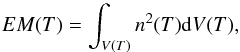 (1)where n(T) is the plasma density at the temperature T, the integration only includes the volume of the grid cells at that particular temperature, and the volume covers all the closed field line regions in the steady-state solutions. We used temperature bins of 0.1 in log T starting from the base temperature (i.e. log T ≃ 4.9) up to the highest temperature achieved in each simulation. Figure 10 contains the computed EM(T) for all the considered cases. As expected, the peak values are located at log T> 6.0, and move towards larger emission measures and higher temperatures with increasing average (radial) magnetic energy density ⟨εB r⟩ (see Table 1).
In a similar manner to the solar case (Sect. 4.1), we compared the simulated quantities to observational values. The ZDI and SH-ZDI simulations of HD 22049 yield maximum EM values of log EM ≃ 49.1 (at log T ≃ 6.4) and log EM ≃ 50.0 (at log T ≃ 6.6), respectively. The peak temperature and emission measure of the ZDI model are lower than those derived from both EUV and X-ray spectra (log EM ≃ 50.7 at log T ≃ 6.6 ± 0.05, Drake et al. 2000; Sanz-Forcada et al. 2004; Ness & Jordan 2008). The SH-ZDI emission measure fares somewhat better, with good agreement in terms of the peak temperature. However, this model still predicts an emission measure significantly lower than observed, by roughly a factor of 5.
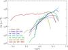 |
Fig. 10 Emission measure distributions EM(T) calculated from the 3D steady-state solutions. Each colour corresponds to one of the simulations presented in Sect. 4, including the solar runs (Appendix A). |
For HD 147513 available observations, from the broad-band filters of the Extreme Ultraviolet Explorer (EUVE) Deep Survey telescope, only provide rough estimates of the coronal conditions, suggesting a probable emission measure in the range log EM ~ 51–52 (Vedder et al. 1993), but with no distinction on the temperature. In turn, the peak of the simulated distribution is located at log T ≃ 6.5, with an associated value of log EM ≃ 49.7. The discrepancy in emission measure might be expected given the relatively low spatial resolution of the SH-ZDI map driving the simulation (Sects. 2 and 4.4). The peak temperature is also slightly lower than what might be expected based on the emission measure distribution and the observed peak temperature of HD 22049.
There are no observational constraints in the literature for HD 1237 regarding the EM distribution. From the numerical simulations, we obtain peak values of log EM ≃ 49.3 at log T ~ 6.5 for the ZDI case, and log EM ≃ 50.2 at log T ~ 6.7 for the SH-ZDI case.
In all the stellar cases, the simulated EM distributions show maxima close to the expected values for stars within the considered levels of activity (see Table 1). However, the emission measures are systematically lower than indicated by observation.
The behaviour of the simulated EM distribution for the solar maximum case (red line in Fig. 10) is particularly interesting compared with the remaining simulations. Both the peak emission measure and temperature agree well with assessments from full solar disk observations (e.g. Laming et al. 1995; Drake et al. 2000). However, the observations indicate a slope in the EM vs. temperature of the order of unity or greater, whereas the model prediction is much flatter. This results in a substantial over-prediction of the cooler emission measure at temperatures log T ≤ 6 compared with observations. The solar minimum EM distribution (yellow line in Fig. 10) is more similar to the stellar cases in this regard. These differences have a considerable impact on the predicted coronal emission, as discussed in the next section.
5.2. High-Energy emission and magnetic flux
An observational study performed by Pevtsov et al. (2003) showed a relation between the unsigned magnetic field flux, ΦB, and the X-ray emission, LX, covering several orders of magnitude in both quantities ( ). The analysis included various magnetic features of the Sun, together with Zeeman broadening (ZB) measurements of active dwarfs (spectral types F, G, and K), and pre-main sequence stars (see Saar 1996). More recently, Vidotto et al. (2014) investigated the behaviour of various astrophysical quantities, including LX, with respect to the large-scale magnetic field flux (recovered with ZDI). They also found a power-law relation for both parameters (
 ). These observational results have been interpreted as an indication of a similar coronal heating mechanism among these types of stars.
In this context, we considered this relation from a numerical point of view by simulating the coronal high-energy emission (based on the EM(T) distributions presented in the previous section) and comparing the predicted fluxes with the underlying surface magnetic field flux distributions ( ). In this analysis, we included the results from all the considered cases (e.g. solar and ZDI/SH-ZDI), treating the solutions independently. This allowed us to explore a broad range for both parameters while maintaining the considerations and limitations of the data-driven numerical approach. In principle, this can also be studied from a more generic numerical point of view (i.e. including different simulated field distributions). However, this would require implicit assumptions about the field strength and spatial configuration (mostly influenced by the solar case), which would introduce strong biases in the analysis. Considering the different recovered field maps (e.g. ZDI/SH-ZDI) as independent observations therefore represents a reasonable approximation.
Spectra were simulated for each of the emission measure distributions, EM(T) over the X-ray and EUV wavelength regimes from 1 to 1100 Å on a 0.1 Å grid, covering all the bandpasses of interest to this work. Emissivities were computed using atomic data from the CHIANTI database version 7.1.4 (Dere et al. 1997; Landi et al. 2013) as implemented in the Package for INTeractive Analysis of Line Emission (PINTofALE)8. The radiative loss in the temperature range of interest for the stars in this study is dominated by metals – principally Si, Mg, and Fe – and the chemical abundance mixture has a concomitant influence on the predicted EUV and X-ray fluxes. HD 22049 and other intermediate-activity G and K dwarfs exhibit a solar-like “first ionization potential effect” in which elements with low first ionization potentials (≤13.6 eV) can be enhanced by factors of up to 4 in the corona relative to photospheric values (e.g. Laming et al. 1996; Wood & Linsky 2010). For the purposes of this study we did not try to match these abundances, but instead adopted the solar abundance mixture of Grevesse & Sauval (1998) as a standard reference set. Fluxes in the different bandpasses discussed below were obtained by integrating the synthetic spectra within the wavelength limits of interest.
Figure 11 shows the relation between the simulated high-energy coronal emission and the unsigned magnetic flux from the radial magnetic field maps. The latter, noted as ⟨ΦBr⟩s, was averaged over the entire surface of the star. The colours correspond to the spectral ranges used for the integration, covering the SXR (2−30 Å, green), X-ray (5−100 Å, red), and EUV (100−920 Å, blue) bands. As indicated, a power-law fit was applied to each channel (continuous lines), while the segmented lines correspond to the previous observational results from Pevtsov et al. (2003) and Vidotto et al. (2014)9. Two vertical arrows in the upper X-axis denote the results for the solar case (⊙ Min and ⊙ Max).
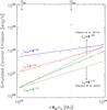 |
Fig. 11 Simulated high-energy coronal emission vs. unsigned radial magnetic flux ⟨ΦBr⟩s. Each point corresponds to one of the simulations described in Sect. 4, including the solar cases as indicated. These values are calculated from synthetic spectra, based on the EM(T) distributions (Sect. 5.1), and integrated in the SXR (2−30 Å, green), X-ray (5−100 Å, red) and EUV (100−920 Å, blue) bands. The solid lines correspond to fits to the simulated data points. The dashed lines are based on observational studies using X-ray, against magnetic field measurements using ZB (Pevtsov et al. 2003) and ZDI (Vidotto et al. 2014). |
Several aspects of Fig. 11 are noteworthy. First, despite the reduced range in ⟨ΦBr⟩s, we were able to retrieve a similar behaviour between radiative flux and magnetic flux as in previous observational studies with larger datasets. For the simulated X-ray range, the results are consistent with the relation obtained by Pevtsov et al. (2003), while in the SXR range the power-law dependance is more similar to the results obtained by Vidotto et al. (2014). This reinforces the applicability of the model, at least to the levels of magnetic activity considered here. In addition, there appears to be a trend towards a steeper relation with increasing energy – from ∝Φ0.5 in the EUV, to ∝Φ1.06−1.52 in the X-ray and SXR ranges. In agreement with observations (Mathioudakis et al. 1995), Fig. 11 shows that the X-ray emission will match and eventually dominate the EUV emission, at higher levels of magnetic activity (and associated magnetic flux). This is also qualitatively consistent with the spectral modelling values reported by Chadney et al. (2015) in terms of the surface fluxes, FX , and FEUV. According to their results, this should occur at activity levels slightly higher than those displayed by HD 22049. This behaviour may be connected with the appearance of strong azimuthal or toroidal fields in the large-scale field of these stars, as in the case of HD 1237 (see Alvarado-Gómez et al. 2015, and references therein).
Comparing the synthetic flux results with observations and spectral modelling data (within the same energy ranges) published by Sanz-Forcada et al. (2011) reveals underestimated values in our models for LX and LEUV. At best, the discrepancy is lower than a factor of 2 in both energy bands, as in the case of the SH-ZDI solution of HD 22049. However, these differences can range up to ~1−2 orders of magnitude in some of our other stellar simulations. The largest discrepancies appear in the EUV band, reflecting the model emission measure deficiencies noted previously. Several observational and numerical factors could give rise to the relatively large mismatch of the results. These include instrumental and signal-to-noise ratio (S/N) effects in the EUV/X-ray observations (see Sanz-Forcada et al. 2011), the spatial resolution and missing flux in the ZDI reconstruction (see Arzoumanian et al. 2011; Lang et al. 2014), temporal incoherence (connected with long-term variations associated with magnetic cycles), and the coronal heating model assumed, among others. Previous numerical studies have adjusted the thermodynamic base conditions to match the peak of the observed EM(T) distribution (Vidotto et al. 2012), or the X-ray luminosity (Llama et al. 2013). However, as the dominant coronal emission changes with the magnetic activity of the star (Mathioudakis et al. 1995; Chadney et al. 2015), this has to be performed in all high-energy bands for a consistent calibration. Despite the various problems and limitations, these comparisons serve as a benchmark to improve this data-driven approach and make it more reliable in stars different from the Sun.
 |
Fig. 12 Spatial distribution of the surface radial magnetic flux ΦBr. The average surface magnetic flux increases from left to right, showing the Sun (Min), HD 1237 (ZDI), Sun (Max), and HD 147513 (SH-ZDI). The degree of complexity is clearly higher in the solar maximum case despite the degraded spatial resolution. The perspective is preserved in all cases with an inclination angle of i = 60°. |
Finally, while both solar cases agree well with observed mean coronal temperatures and high-energy emission (see Sect. 4.1), the activity maximum solution appears far higher than the general trends in both the EUV and X-ray, as shown in Fig. 11. By removing these points from the power-law fits, the scatter is reduced considerably (by a factor of ~5 in the EUV and ~2.5 in the X-ray). This is directly connected with the resulting shape of the EM(T) distribution, presented in Sect. 5.1, which is much flatter than observed. Consequently, the EUV flux is much higher by a commensurate margin than the solar minimum and the stellar counterparts. The “cool” plasma excess is related to the response of the coronal model heating law to the field topology and associated complexity (see Sect. 2). To show this in more detail, we compare the surface distribution of ΦBr of four of the cases considered in ascending order of ⟨ΦBr⟩s (Fig. 12). Even with a degraded resolution, the solar maximum case contains a far more complex field distribution than in any of our ZDI models. This makes the comparison between the solar activity maximum case and ZDI-driven models extremely difficult. From this perspective, the solar minimum state provides a more suitable point of comparison for ZDI-based stellar studies. Indeed, the predicted fluxes for the solar minimum case are well-aligned with the power-law fits in Fig. 11.
5.3. Coronal features and rotational modulation
In this last section we calculate the rotational modulation of the high-energy emission that is due to the specific coronal features developed in the simulation. The stellar emission in the X-ray and EUV ranges plays a fundamental role in the thermal structure and dynamical evolution of planetary atmospheres (see Lammer et al. 2003; Lammer 2013). Processes such as heating of the exospheres or thermospheres, expansion, and atmospheric escape are highly sensitive to these parameters (Lammer et al. 2008; Guo 2011; Shaikhislamov et al. 2014). However, there are several observational difficulties, particularly in the EUV, in accessing these ranges of the electromagnetic spectrum, such as lack of instrumentation and strong absorption by the interstellar medium (Chadney et al. 2015). Various alternatives have been used to overcome these issues, including extrapolations based on average solar EUV fluxes (Lecavelier Des Etangs 2007), coronal models from spectral synthesis (Sanz-Forcada et al. 2011), and predictions from rotational evolution models (Tu et al. 2015). Still, these procedures are not able to estimate the variability on time-scales comparable to the stellar rotation period, or from the geometrical configuration of the system (e.g. orbital inclination). Both elements can be considered in our data-driven numerical approach, provided that the entire 3D structure of the corona is generated. These factors can have important effects on exoplanetary conditions such as climate patterns and habitability (e.g. Forget & Leconte 2014) and on the detectability of transits either in X-ray (Poppenhaeger et al. 2013) or near-UV wavelengths (Haswell et al. 2012; Llama et al. 2011).
For this purpose, we used the system analysed here that is the most extreme in terms of high-energy emission and proximity of the planet. This corresponds to HD 1237 using the SH-ZDI field distribution (Fig. 6, see also Table 1). From the steady-state coronal solution, we generated a set of synthetic high-energy emission maps covering an entire rotation of the star, with three different line-of-sight angles (30, 60, and 90°)10. Figure 13 contains the resulting rotational modulation of the coronal emission for each of the considered inclinations. These variations are induced by the different coronal features described in Sect. 4.2. Around 0.2 and 0.8 in rotational phase, the large coronal holes cross the stellar disk, while at Φ = 0.5 and Φ = 1.0, they are located near the limb (close to the perspective presented in Fig. 6).
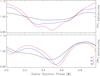 |
Fig. 13 Rotational modulation of the high-energy coronal emission for HD 1237 (SH-ZDI), showing the EUV (top) and SXR (bottom) ranges. Colours indicate the inclination angle used for the calculation. |
As expected, the high-energy modulation is reduced for smaller inclination angles (e.g. closer to a pole-on view); it is lower than 5% of the mean value for both energy bands. For larger inclinations, the modulation increases, reaching up to ~15% in the 90° inclination case. These values are fully consistent with the X-ray modulation estimates in the HD 189733 (K2V) system obtained by Llama et al. (2013), which displays a comparable field strength at the stellar surface (~± 30 G).
Depending on the magnetic field evolution, the modulation of the coronal emission could persist for time-scales longer than one rotation period of the star. This is the case for HD 1237, where the large-scale field seems stable on a time-scale of months (Alvarado-Gómez et al. 2015). A fraction of the coronal emission may show rotational modulation on time-scales comparable to the orbital period of the exoplanet (Porb = 133.7 ± 0.2 days, Naef et al. 2001). However, an additional component will be due to shorter term reconnection events (e.g. flares). Furthermore, as the planetary system has a high orbital eccentricity (e ≃ 0.5), any X-ray and EUV rotational modulation will most likely play a secondary role in terms of the irradiation environment. This will be considered in the second paper of this study, in combination with the influence of the magnetized stellar wind on the exoplanetary conditions.
A similar approach can be followed in other systems, provided ZDI reconstructions are available for the host star (see Fares et al. 2013). More complex scenarios are expected in hot-Jupiters, where the orbital period can be equal to or even shorter than the stellar rotation period. One example is the HD 179949 (F8V) system (Fares et al. 2012), where planet-induced coronal activity has been suggested (Shkolnik et al. 2008). Still, recent multi-wavelength observations of this system presented by Scandariato et al. (2013) appear to be consistent with rotational modulation alone. Nevertheless, this does not exclude the possibility of star-planet interactions in the system, which could be explored in more detail with the data-driven approach presented in this paper. Moreover, as has been shown by Cohen et al. (2011), it is also possible to simulate in detail space weather phenomena, such as coronal mass ejections, in these extreme exoplanetary systems.
6. Summary and conclusions
We have performed a detailed numerical simulation of the 3D coronal structure of three late-type planet-hosting stars (HD 1237, HD 22049, and HD 147513). A steady-state solution was calculated self-consistently, driven by the surface magnetic field distributions recovered with the technique of Zeeman-Doppler imaging. The main results of our study are summarised below.
We compared the coronal solutions driven by two similarimplementations of this mapping technique (ZDI and SH-ZDI).The global structure of the resulting corona is consistent in bothcases. A quantitative analysis showed important differences inthe thermodynamic conditions and in the coronal high-energyemission. We obtained differences of up to factors of 1.4 and 2.5 in the coronal temperature and density, respectively. This led to a larger variation in the predicted EUV and SXR emission, reaching up to one order of magnitude. These differences can be related to the amount of structure, field strength, and the map completeness in each case.
The appearance of different coronal features in each star is highly dependent on the characteristics of the surface field distribution. Two large coronal holes appear as the most prominent elements in HD 1237. HD 22049 shows more complex details, displaying additional structures such as helmet streamers and filaments. For HD 147513, the simulation predicts a rather simple coronal topology, reflecting the low-complexity of its surface magnetic field.
Comparable solar simulations in terms of spatial resolution and boundary conditions were considered (covering activity minimum and maximum). This included a detailed comparison with archival satellite data in the EUV and SXR ranges. For both activity states, good agreement was obtained in terms of the coronal temperature (~8% difference) and in the high-energy coronal emission (SXR/EUV bands). On the other hand, the emission measure distribution showed larger discrepancies, with a considerable excess at the low-temperature end (log T< 6.0) for the solar maximum case. In addition, within the temperature range of 1−2 MK, the EM appears underestimated by factors of ~3 and 5 for activity maximum and minimum, respectively. This is likely indicative of the need to recalibrate the coronal heating mechanism when applying this model to resolution-limited surface magnetic field distributions.
Furthermore, while the comparison to the observations showed similar levels of agreement for both solar minimum and maximum cases (e.g. thermodynamic conditions and high-energy emission), the simpler structure of the large-scale magnetic field makes the former a better reference point for simulations based on ZDI maps (see Fig. 12).
We considered the particular case of HD 1237 to estimate the rotational modulation in the high-energy emission that is due to the coronal features developed in our simulation. We obtained variabilities ranging from ~5−15% (depending on the line-of-sight angle) in the mean coronal EUV and SXR emission. Similar estimates have been reported for systems with comparable surface field strengths (e.g. HD 189733, Llama et al. 2013).
In addition, using the simulations, we were able to recover similar trends as in previous observational studies, including a relation between the magnetic flux (ΦBr) and the coronal high-energy emission (Pevtsov et al. 2003; Vidotto et al. 2014). However, as this numerical model was specifically developed for the Sun, further adjustments will be required to better calibrate our results to the stellar data.
Improvements in this approach can be performed by extending the range in ΦBr. This could be done by isolating specific regions from high-resolution solar observations and by expanding the stellar sample to more active stars. For the latter case, it would be necessary to further adjust the coronal heating or the thermodynamic base conditions to match the observed coronal emission in all energy bands. Another possibility would involve a more sophisticated numerical treatment to be able to consider all the magnetic field components to drive the simulation (see Fisher et al. 2015).
The results discussed in this work will be used in a follow-up paper to self-consistently simulate the stellar wind, inner astrosphere, and circumstellar environment of these systems. This includes stellar and planetary mass losses, orbital conditions, and topology of the astrospheric current sheet.
Therefore, for HD 22049 (ϵ Eridani) we only consider the January 2010 dataset (see Piskunov et al. 2011; Jeffers et al. 2014).
Code version 2.4.
Except in the magnetic energy density distribution for the solar minimum case (Fig. A.1), where the range is decreased by a factor of 10.
A quick-look comparison with the observations from various instruments during these dates is provided at http://helioviewer.org/
Available at the Virtual Solar Observatory (VSO).
More information can be found in the EIT user guide.
We shifted the relation from Vidotto et al. (2014) to match the Pevtsov et al. (2003) relation at the solar minimum value. This was performed for comparison purposes, as there are still discrepancies in the absolute values of the observational LX−ΦB relations, most likely connected with the method to estimate the surface magnetic flux (i.e. ZB in Pevtsov et al. 2003; and ZDI in Vidotto et al. 2014).
This angle is measured between the stellar rotation axis and the position of the observer.
Acknowledgments
This work was carried out using the SWMF/BATSRUS tools developed at The University of Michigan Center for Space Environment Modeling (CSEM) and made available through the NASA Community Coordinated Modeling Center (CCMC). We acknowledge the support by the DFG Cluster of Excellence “Origin and Structure of the Universe”. We are grateful for the support by A. Krukau through the Computational Center for Particle and Astrophysics (C2PAP).
References
- Acton, L. W., Weston, D. C., & Bruner, M. E. 1999, J. Geophys. Res., 104, 14827 [NASA ADS] [CrossRef] [Google Scholar]
- Alvarado-Gómez, J. D., Hussain, G. A. J., Grunhut, J., et al. 2015, A&A, 582, A38 [NASA ADS] [CrossRef] [EDP Sciences] [Google Scholar]
- Arzoumanian, D., Jardine, M., Donati, J.-F., Morin, J., & Johnstone, C. 2011, MNRAS, 410, 2472 [NASA ADS] [CrossRef] [Google Scholar]
- Aurière, M. 2003, in EAS PS 9, eds. J. Arnaud, & N. Meunier, 105 [Google Scholar]
- Baliunas, S. L., Donahue, R. A., Soon, W. H., et al. 1995, ApJ, 438, 269 [NASA ADS] [CrossRef] [Google Scholar]
- Benedict, G. F., McArthur, B. E., Gatewood, G., et al. 2006, AJ, 132, 2206 [NASA ADS] [CrossRef] [Google Scholar]
- Boro Saikia, S., Jeffers, S. V., Petit, P., et al. 2015, A&A, 573, A17 [NASA ADS] [CrossRef] [EDP Sciences] [Google Scholar]
- Brown, S. F., Donati, J.-F., Rees, D. E., & Semel, M. 1991, A&A, 250, 463 [NASA ADS] [Google Scholar]
- Chadney, J. M., Galand, M., Unruh, Y. C., Koskinen, T. T., & Sanz-Forcada, J. 2015, Icarus, 250, 357 [NASA ADS] [CrossRef] [Google Scholar]
- Charbonneau, P. 2014, ARA&A, 52, 251 [Google Scholar]
- Cohen, O., & Drake, J. J. 2014, ApJ, 783, 55 [NASA ADS] [CrossRef] [Google Scholar]
- Cohen, O., Drake, J. J., Kashyap, V. L., Hussain, G. A. J., & Gombosi, T. I. 2010, ApJ, 721, 80 [NASA ADS] [CrossRef] [Google Scholar]
- Cohen, O., Kashyap, V. L., Drake, J. J., Sokolov, I. V., & Gombosi, T. I. 2011, ApJ, 738, 166 [NASA ADS] [CrossRef] [Google Scholar]
- Cohen, O., Drake, J. J., Glocer, A., et al. 2014, ApJ, 790, 57 [NASA ADS] [CrossRef] [Google Scholar]
- De Pontieu, B., McIntosh, S. W., Carlsson, M., et al. 2007, Science, 318, 1574 [NASA ADS] [CrossRef] [PubMed] [Google Scholar]
- Dere, K. P., Landi, E., Mason, H. E., Monsignori Fossi, B. C., & Young, P. R. 1997, A&AS, 125, 149 [NASA ADS] [CrossRef] [EDP Sciences] [Google Scholar]
- Domingo, V., Fleck, B., & Poland, A. I. 1995, Sol. Phys., 162, 1 [NASA ADS] [CrossRef] [Google Scholar]
- Donati, J.-F., & Brown, S. F. 1997, A&A, 326, 1135 [NASA ADS] [Google Scholar]
- Donati, J.-F., & Landstreet, J. D. 2009, ARA&A, 47, 333 [NASA ADS] [CrossRef] [MathSciNet] [Google Scholar]
- Donati, J.-F., Howarth, I. D., Jardine, M. M., et al. 2006, MNRAS, 370, 629 [NASA ADS] [CrossRef] [Google Scholar]
- Donati, J.-F., Moutou, C., Farès, R., et al. 2008, MNRAS, 385, 1179 [NASA ADS] [CrossRef] [Google Scholar]
- Donati, J.-F., Hébrard, E., Hussain, G., et al. 2014, MNRAS, 444, 3220 [NASA ADS] [CrossRef] [Google Scholar]
- Drake, J. J., & Smith, G. 1993, ApJ, 412, 797 [NASA ADS] [CrossRef] [Google Scholar]
- Drake, J. J., Peres, G., Orlando, S., Laming, J. M., & Maggio, A. 2000, ApJ, 545, 1074 [NASA ADS] [CrossRef] [Google Scholar]
- Fares, R., Donati, J.-F., Moutou, C., et al. 2009, MNRAS, 398, 1383 [NASA ADS] [CrossRef] [MathSciNet] [Google Scholar]
- Fares, R., Donati, J.-F., Moutou, C., et al. 2012, MNRAS, 423, 1006 [NASA ADS] [CrossRef] [Google Scholar]
- Fares, R., Moutou, C., Donati, J.-F., et al. 2013, MNRAS, 435, 1451 [NASA ADS] [CrossRef] [Google Scholar]
- Favata, F., Micela, G., Orlando, S., et al. 2008, A&A, 490, 1121 [NASA ADS] [CrossRef] [EDP Sciences] [Google Scholar]
- Fisher, G. H., Abbett, W. P., Bercik, D. J., et al. 2015, Space Weather, 13, 369 [NASA ADS] [CrossRef] [Google Scholar]
- Forget, F., & Leconte, J. 2014, Phil. Trans. Roy. Soc. London Ser. A, 372, 30084 [Google Scholar]
- Garraffo, C., Cohen, O., Drake, J. J., & Downs, C. 2013, ApJ, 764, 32 [NASA ADS] [CrossRef] [Google Scholar]
- Grevesse, N., & Sauval, A. J. 1998, Space Sci. Rev., 85, 161 [NASA ADS] [CrossRef] [Google Scholar]
- Guo, J. H. 2011, ApJ, 733, 98 [NASA ADS] [CrossRef] [Google Scholar]
- Haswell, C. A., Fossati, L., Ayres, T., et al. 2012, ApJ, 760, 79 [NASA ADS] [CrossRef] [Google Scholar]
- Hathaway, D. H. 2010, Liv. Rev. Sol. Phys., 7, 1 [Google Scholar]
- Hatzes, A. P., Cochran, W. D., McArthur, B., et al. 2000, ApJ, 544, L145 [NASA ADS] [CrossRef] [Google Scholar]
- Hussain, G. A. J., Jardine, M., & Collier Cameron, A. 2001, MNRAS, 322, 681 [NASA ADS] [CrossRef] [Google Scholar]
- Hussain, G. A. J., Collier Cameron, A., Jardine, M. M., et al. 2009, MNRAS, 398, 189 [NASA ADS] [CrossRef] [Google Scholar]
- Hussain, G. A. J., Alvarado-Gómez, J. D., Grunhut, J., et al. 2016, A&A, 585, A77 [NASA ADS] [CrossRef] [EDP Sciences] [Google Scholar]
- Jeffers, S. V., Petit, P., Marsden, S. C., et al. 2014, A&A, 569, A79 [NASA ADS] [CrossRef] [EDP Sciences] [Google Scholar]
- Johnstone, C., Jardine, M., & Mackay, D. H. 2010, MNRAS, 404, 101 [NASA ADS] [Google Scholar]
- Jordan, C. 1975, MNRAS, 170, 429 [NASA ADS] [CrossRef] [Google Scholar]
- Judge, P. G., Solomon, S. C., & Ayres, T. R. 2003, ApJ, 593, 534 [NASA ADS] [CrossRef] [Google Scholar]
- Kochukhov, O., & Wade, G. A. 2010, A&A, 513, A13 [NASA ADS] [CrossRef] [EDP Sciences] [Google Scholar]
- Laming, J. M., Drake, J. J., & Widing, K. G. 1995, ApJ, 443, 416 [NASA ADS] [CrossRef] [Google Scholar]
- Laming, J. M., Drake, J. J., & Widing, K. G. 1996, ApJ, 462, 948 [NASA ADS] [CrossRef] [Google Scholar]
- Lammer, H. 2013, Origin and Evolution of Planetary Atmospheres (Berlin, Heidelberg: Springer) [Google Scholar]
- Lammer, H., Selsis, F., Ribas, I., et al. 2003, ApJ, 598, L121 [NASA ADS] [CrossRef] [Google Scholar]
- Lammer, H., Kasting, J. F., Chassefière, E., et al. 2008, Space Sci. Rev., 139, 399 [NASA ADS] [CrossRef] [Google Scholar]
- Landi, E., Young, P. R., Dere, K. P., Del Zanna, G., & Mason, H. E. 2013, ApJ, 763, 86 [NASA ADS] [CrossRef] [Google Scholar]
- Lang, P., Jardine, M., Morin, J., et al. 2014, MNRAS, 439, 2122 [NASA ADS] [CrossRef] [Google Scholar]
- Lecavelier Des Etangs, A. 2007, A&A, 461, 1185 [NASA ADS] [CrossRef] [EDP Sciences] [Google Scholar]
- Llama, J., Wood, K., Jardine, M., et al. 2011, MNRAS, 416, L41 [NASA ADS] [CrossRef] [Google Scholar]
- Llama, J., Vidotto, A. A., Jardine, M., et al. 2013, MNRAS, 436, 2179 [NASA ADS] [CrossRef] [Google Scholar]
- Mathioudakis, M., Fruscione, A., Drake, J. J., et al. 1995, A&A, 300, 775 [NASA ADS] [Google Scholar]
- Mayor, M., Pepe, F., Queloz, D., et al. 2003, The Messenger, 114, 20 [NASA ADS] [Google Scholar]
- Mayor, M., Udry, S., Naef, D., et al. 2004, A&A, 415, 391 [NASA ADS] [CrossRef] [EDP Sciences] [Google Scholar]
- McIntosh, S. W., de Pontieu, B., Carlsson, M., et al. 2011, Nature, 475, 477 [NASA ADS] [CrossRef] [Google Scholar]
- Morgenthaler, A., Petit, P., Saar, S., et al. 2012, A&A, 540, A138 [NASA ADS] [CrossRef] [EDP Sciences] [Google Scholar]
- Moses, D., Clette, F., Delaboudinière, J.-P., et al. 1997, Sol. Phys., 175, 571 [NASA ADS] [CrossRef] [Google Scholar]
- Naef, D., Mayor, M., Pepe, F., et al. 2001, A&A, 375, 205 [NASA ADS] [CrossRef] [EDP Sciences] [Google Scholar]
- Ness, J.-U., & Jordan, C. 2008, MNRAS, 385, 1691 [NASA ADS] [CrossRef] [Google Scholar]
- Pesnell, W. D., Thompson, B. J., & Chamberlin, P. C. 2012, Sol. Phys., 275, 3 [NASA ADS] [CrossRef] [Google Scholar]
- Petit, P., Dintrans, B., Solanki, S. K., et al. 2008, MNRAS, 388, 80 [NASA ADS] [CrossRef] [MathSciNet] [Google Scholar]
- Petit, P., Dintrans, B., Morgenthaler, A., et al. 2009, A&A, 508, L9 [NASA ADS] [CrossRef] [EDP Sciences] [Google Scholar]
- Pevtsov, A. A., Fisher, G. H., Acton, L. W., et al. 2003, ApJ, 598, 1387 [NASA ADS] [CrossRef] [Google Scholar]
- Pietarila, A., & Judge, P. G. 2004, ApJ, 606, 1239 [NASA ADS] [CrossRef] [Google Scholar]
- Piskunov, N., & Kochukhov, O. 2002, A&A, 381, 736 [NASA ADS] [CrossRef] [EDP Sciences] [Google Scholar]
- Piskunov, N., Snik, F., Dolgopolov, A., et al. 2011, The Messenger, 143, 7 [NASA ADS] [Google Scholar]
- Poppenhaeger, K., Schmitt, J. H. M. M., & Wolk, S. J. 2013, ApJ, 773, 62 [NASA ADS] [CrossRef] [Google Scholar]
- Powell, K. G., Roe, P. L., Linde, T. J., Gombosi, T. I., & De Zeeuw, D. L. 1999, J. Comp. Phys., 154, 284 [NASA ADS] [CrossRef] [Google Scholar]
- Robrade, J., Schmitt, J. H. M. M., & Favata, F. 2012, A&A, 543, A84 [NASA ADS] [CrossRef] [EDP Sciences] [Google Scholar]
- Saar, S. H. 1996, in Stellar Surface Structure, eds. K. G. Strassmeier, & J. L. Linsky, IAU Symp., 176, 237 [Google Scholar]
- Sanz-Forcada, J., Favata, F., & Micela, G. 2004, A&A, 416, 281 [NASA ADS] [CrossRef] [EDP Sciences] [Google Scholar]
- Sanz-Forcada, J., Micela, G., Ribas, I., et al. 2011, A&A, 532, A6 [NASA ADS] [CrossRef] [EDP Sciences] [Google Scholar]
- Scandariato, G., Maggio, A., Lanza, A. F., et al. 2013, A&A, 552, A7 [NASA ADS] [CrossRef] [EDP Sciences] [Google Scholar]
- Scherrer, P. H., Bogart, R. S., Bush, R. I., et al. 1995, Sol. Phys., 162, 129 [Google Scholar]
- Semel, M. 1989, A&A, 225, 456 [NASA ADS] [Google Scholar]
- Shaikhislamov, I. F., Khodachenko, M. L., Sasunov, Y. L., et al. 2014, ApJ, 795, 132 [NASA ADS] [CrossRef] [Google Scholar]
- Shkolnik, E., Bohlender, D. A., Walker, G. A. H., & Collier Cameron, A. 2008, ApJ, 676, 628 [NASA ADS] [CrossRef] [Google Scholar]
- Sokolov, I. V., van der Holst, B., Oran, R., et al. 2013, ApJ, 764, 23 [NASA ADS] [CrossRef] [Google Scholar]
- Tóth, G., van der Holst, B., Sokolov, I. V., et al. 2012, J. Comp. Phys., 231, 870 [CrossRef] [Google Scholar]
- Tu, L., Johnstone, C. P., Güdel, M., & Lammer, H. 2015, A&A, 577, L3 [NASA ADS] [CrossRef] [EDP Sciences] [Google Scholar]
- van der Holst, B., Sokolov, I. V., Meng, X., et al. 2014, ApJ, 782, 81 [Google Scholar]
- Vedder, P. W., Patterer, R. J., Jelinsky, P., Brown, A., & Bowyer, S. 1993, ApJ, 414, L61 [NASA ADS] [CrossRef] [Google Scholar]
- Vidotto, A. A., Jardine, M., Opher, M., Donati, J. F., & Gombosi, T. I. 2011, MNRAS, 412, 351 [NASA ADS] [CrossRef] [Google Scholar]
- Vidotto, A. A., Fares, R., Jardine, M., et al. 2012, MNRAS, 423, 3285 [NASA ADS] [CrossRef] [Google Scholar]
- Vidotto, A. A., Gregory, S. G., Jardine, M., et al. 2014, MNRAS, 441, 2361 [NASA ADS] [CrossRef] [Google Scholar]
- Vidotto, A. A., Fares, R., Jardine, M., Moutou, C., & Donati, J.-F. 2015, MNRAS, 449, 4117 [NASA ADS] [CrossRef] [Google Scholar]
- Wood, B. E., & Linsky, J. L. 2010, ApJ, 717, 1279 [NASA ADS] [CrossRef] [Google Scholar]
Appendix A: Simulation results for the Sun
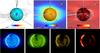 |
Fig. A.1 Simulation results for the coronal structure of the Sun during activity minimum (CR 1922). The upper panels contain the distribution of the magnetic energy density (εB r, left), the number density (n, middle) and temperature (T, right). For the last two quantities, the distribution over the plane y = 0 is presented. The sphere represents the stellar surface and selected 3D magnetic field lines are shown in white. Note the change of scale for εB r in this case. The lower images correspond to synthetic coronal emission maps in EUV (blue/171 Å, green/195 Å, and yellow/284 Å) and SXR (red/2−30 Å). The perspective is preserved in all panels, with an inclination angle of i = 90 °. |
 |
Fig. A.2 Simulation results for the coronal structure of the Sun during activity maximum (CR 1962). See caption of Fig. A.1. |
All Tables
Average physical properties of the inner corona (IC) region (from 1.05 to 1.5 R∗).
All Figures
|
Fig. 1 Surface radial magnetic field maps of HD 1237. A comparison between the standard ZDI (top) and the SH-ZDI (bottom) is presented. The colour scale indicates the polarity and the field strength in Gauss (G). Note the difference in the magnetic field range for each case. The stellar inclination angle (i = 50°) is used for the visualisations. |
| In the text | |
|
Fig. 2 Surface radial magnetic field maps of HD 22049. See caption of Fig. 1. The stellar inclination angle (i = 45°) is used for the visualisations. |
| In the text | |
|
Fig. 3 Surface radial magnetic field maps of HD 147513 using SH-ZDI. Two rotational phases (Φ) are presented. The stellar inclination angle (i = 20°) is used for the visualisations. |
| In the text | |
|
Fig. 4 Surface radial magnetic field maps of the Sun during activity minimum (CR 1922, top) and maximum (CR 1962, bottom) taken by SOHO/MDI. Note the difference in the magnetic field range for each case. An inclination angle i = 90° is used for the visualisations. |
| In the text | |
|
Fig. 5 Simulation results for the coronal structure of HD 1237 driven by the ZDI large-scale magnetic field map. The upper panels contain the distribution of the magnetic energy density (εB r, left), the number density (n, middle), and temperature (T, right). For the last two quantities the distribution over the equatorial plane (z = 0) is presented. The sphere represents the stellar surface and selected 3D magnetic field lines are shown in white. The lower images correspond to synthetic coronal emission maps in EUV (blue/171 Å, green/195 Å and yellow/284 Å) and SXR (red/2−30 Å). The perspective and colour scales are preserved in all panels, with an inclination angle of i = 50 °. |
| In the text | |
|
Fig. 6 Simulation results for the coronal structure of HD 1237 driven by the SH-ZDI large-scale field map. See caption of Fig. 5. The 3D magnetic field lines are calculated in the same spatial locations as in the solution presented in Fig. 5. |
| In the text | |
|
Fig. 7 Simulation results for the coronal structure of HD 22049 driven by the ZDI large-scale magnetic field map. The upper panels contain the distribution of the magnetic energy density (εB r, left), the number density (n, middle), and temperature (T, right). For the last two quantities the distribution over the equatorial plane (z = 0) is presented. The sphere represents the stellar surface and selected 3D magnetic field lines are shown in white. The lower images correspond to synthetic coronal emission maps in EUV (blue/171 Å, green/195 Å and yellow/284 Å) and SXR (red/2−30 Å). The perspective and colour scales are preserved in all panels, with an inclination angle of i = 45°. |
| In the text | |
|
Fig. 8 Simulation results for the coronal structure of HD 22049 driven by the SH-ZDI large-scale field map. See caption of Fig. 7. The 3D magnetic field lines are calculated in the same spatial locations as in the solution presented in Fig. 7. |
| In the text | |
|
Fig. 9 Simulation results for the coronal structure of HD 147513 driven by the SH-ZDI large-scale magnetic field map. The upper panels contain the distribution of the magnetic energy density (εB r, left), the number density (n, middle), and temperature (T, right). For the last two quantities the distribution over the equatorial plane (z = 0) is presented. The sphere represents the stellar surface and selected 3D magnetic field lines are shown in white. The lower images correspond to synthetic coronal emission maps in EUV (blue/171 Å, green/195 Å and yellow/284 Å) and SXR (red/2−30 Å). The perspective is preserved in all panels, with an inclination angle of i = 20°. |
| In the text | |
|
Fig. 10 Emission measure distributions EM(T) calculated from the 3D steady-state solutions. Each colour corresponds to one of the simulations presented in Sect. 4, including the solar runs (Appendix A). |
| In the text | |
|
Fig. 11 Simulated high-energy coronal emission vs. unsigned radial magnetic flux ⟨ΦBr⟩s. Each point corresponds to one of the simulations described in Sect. 4, including the solar cases as indicated. These values are calculated from synthetic spectra, based on the EM(T) distributions (Sect. 5.1), and integrated in the SXR (2−30 Å, green), X-ray (5−100 Å, red) and EUV (100−920 Å, blue) bands. The solid lines correspond to fits to the simulated data points. The dashed lines are based on observational studies using X-ray, against magnetic field measurements using ZB (Pevtsov et al. 2003) and ZDI (Vidotto et al. 2014). |
| In the text | |
|
Fig. 12 Spatial distribution of the surface radial magnetic flux ΦBr. The average surface magnetic flux increases from left to right, showing the Sun (Min), HD 1237 (ZDI), Sun (Max), and HD 147513 (SH-ZDI). The degree of complexity is clearly higher in the solar maximum case despite the degraded spatial resolution. The perspective is preserved in all cases with an inclination angle of i = 60°. |
| In the text | |
|
Fig. 13 Rotational modulation of the high-energy coronal emission for HD 1237 (SH-ZDI), showing the EUV (top) and SXR (bottom) ranges. Colours indicate the inclination angle used for the calculation. |
| In the text | |
|
Fig. A.1 Simulation results for the coronal structure of the Sun during activity minimum (CR 1922). The upper panels contain the distribution of the magnetic energy density (εB r, left), the number density (n, middle) and temperature (T, right). For the last two quantities, the distribution over the plane y = 0 is presented. The sphere represents the stellar surface and selected 3D magnetic field lines are shown in white. Note the change of scale for εB r in this case. The lower images correspond to synthetic coronal emission maps in EUV (blue/171 Å, green/195 Å, and yellow/284 Å) and SXR (red/2−30 Å). The perspective is preserved in all panels, with an inclination angle of i = 90 °. |
| In the text | |
|
Fig. A.2 Simulation results for the coronal structure of the Sun during activity maximum (CR 1962). See caption of Fig. A.1. |
| In the text | |
Current usage metrics show cumulative count of Article Views (full-text article views including HTML views, PDF and ePub downloads, according to the available data) and Abstracts Views on Vision4Press platform.
Data correspond to usage on the plateform after 2015. The current usage metrics is available 48-96 hours after online publication and is updated daily on week days.
Initial download of the metrics may take a while.