| Issue |
A&A
Volume 688, August 2024
|
|
|---|---|---|
| Article Number | A63 | |
| Number of page(s) | 13 | |
| Section | Stellar structure and evolution | |
| DOI | https://doi.org/10.1051/0004-6361/202449581 | |
| Published online | 02 August 2024 | |
Spectropolarimetric characterisation of exoplanet host stars in preparation of the Ariel mission
Magnetic environment of HD 63433
1
Leiden Observatory, Leiden University, PO Box 9513 2300 RA Leiden, The Netherlands
e-mail: This email address is being protected from spambots. You need JavaScript enabled to view it.
2
Institut de Recherche en Astrophysique et Planétologie, Université de Toulouse, CNRS, IRAP/UMR 5277, 14 Avenue Edouard Belin, 31400 Toulouse, France
3
Science Division, Directorate of Science, European Space Research and Technology Centre (ESA/ESTEC), Keplerlaan 1, 2201 AZ Noordwijk, The Netherlands
4
Laboratoire Univers et Particules de Montpellier, Université de Montpellier, CNRS, 34095 Montpellier, France
5
University of Vienna, Department of Astrophysics, Türkenschanzstrasse 17, 1180 Vienna, Austria
6
INAF – Osservatorio Astrofisico di Arcetri, Largo E. Fermi 5, 50125 Firenze, Italy
7
INAF – Osservatorio Astronomico di Palermo, Piazza del Parlamento 1, 90134 Palermo, Italy
Received:
12
February 2024
Accepted:
15
May 2024
Abstract
Context. The accurate characterisation of the stellar magnetism of planetary host stars has been gaining momentum, especially in the context of transmission spectroscopy investigations of exoplanets. Indeed, the magnetic field regulates the amount of energetic radiation and stellar wind impinging on planets, as well as the presence of inhomogeneities on the stellar surface that hinder the precise extraction of the planetary atmospheric absorption signal.
Aims. We initiated a spectropolarimetric campaign to unveil the magnetic field properties of known exoplanet hosting stars included in the current list of potential Ariel targets. In this work, we focus on HD 63433, a young solar-like star hosting two sub-Neptunes and an Earth-sized planet. These exoplanets orbit within 0.15 au from the host star and have likely experienced different atmospheric evolutionary paths.
Methods. We analysed optical spectropolarimetric data collected with ESPaDOnS, HARPSpol, and Neo-Narval to compute the magnetic activity indices ( , Hα, and Ca II infrared triplet), measure the longitudinal magnetic field, and reconstruct the large-scale magnetic topology via Zeeman-Doppler imaging (ZDI). The magnetic field map was then employed to simulate the space environment in which the exoplanets orbit.
Results. The reconstructed stellar magnetic field has an average strength of 24 G and it features a complex topology with a dominant toroidal component, in agreement with other stars of a similar spectral type and age. Our simulations of the stellar environment locate 10% of the innermost planetary orbit inside the Alfvén surface and, thus, brief magnetic connections between the planet and the star can occur. The outer planets are outside the Alfvén surface and a bow shock between the stellar wind and the planetary magnetosphere could potentially form.
Key words: techniques: polarimetric / stars: activity / stars: magnetic field / stars: individual: HD 63433
© ESO 2024
 Open Access article, published by EDP Sciences, under the terms of the Creative Commons Attribution License (http://creativecommons.org/licenses/by/4.0), which permits unrestricted use, distribution, and reproduction in any medium, provided the original work is properly cited.
1. Introduction
The field of exoplanetology has flourished significantly over the past three decades. With more than 5500 confirmed detections1, the main goal is to progressively focus on a comprehensive characterisation of the planetary population. Our knowledge of planet formation and evolution will indeed progress by inspecting the chemical variety of exoplanet atmospheres and, in turn, it will allow us to constrain planet formation theories and refine the assessment framework of potential biomarkers. These considerations motivated the deployment of space-based missions currently in operation such as JWST (Gardner et al. 2006), as well as future ones such as Ariel (Tinetti et al. 2021), which is a medium-class science mission planned for launch by the European Space Agency in 2029. It will target a comprehensive and diverse sample of telluric, ocean, and gas giant planets discovered primarily via radial velocities and transit photometry, orbiting around stars of all accessible spectral types, from early A to late M (Zingales et al. 2018; Edwards et al. 2019; Edwards & Tinetti 2022) types.
When it comes to atmospheric characterisation surveys of exoplanets, stellar magnetic activity is a crucial aspect that ought to be taken into account to avoid wrongful or biased interpretations of the planetary nature. In fact, stellar activity is responsible for photospheric inhomogeneities such as spots and faculae, to which the optical and near-infrared (NIR) are sensitive within the spectral ranges commonly examined for exoplanet detection and characterisation. These inhomogeneities contaminate radial velocity signals (e.g. Huélamo et al. 2008; Dumusque et al. 2011), either mimicking a planetary signal (e.g. Carmona et al. 2023) or preventing an accurate estimation of the planetary mass, ultimately affecting a correct atmospheric retrieval (Changeat et al. 2020; Di Maio et al. 2023). In the case of transmission spectroscopy, stellar activity can bias the observed spectrum, causing the transit chord to differ from the disk-integrated stellar spectrum, generating ambiguity in the extraction of the planetary atmospheric absorption signal (e.g. Rackham et al. 2018, 2019; Salz et al. 2018). For instance, spots affect the transit depth with at least the same order of magnitude as transiting exoplanets, potentially emulating the presence of specific chemical species like H2O (Rackham et al. 2018). Therefore, designing activity-filtering techniques for transmission spectroscopy is necessary (Cracchiolo et al. 2021; Thompson et al. 2024).
In addition, magnetic activity shapes the environment in which exoplanets orbit, and it affects their atmospheres, especially during the early stages of their formation (e.g. Ribas et al. 2005; Allan & Vidotto 2019; Ketzer & Poppenhaeger 2023). Strong activity can endanger habitability (e.g., Airapetian et al. 2017; Tilley et al. 2019), as it indeed correlates with energetic phenomena, such as flares, ultimately modifying the atmospheric chemical composition (Segura et al. 2010; Guenther & Kislyakova 2020; Konings et al. 2022; Louca et al. 2023. Ionising radiation (e.g. in the extreme-ultraviolet and X-rays) and particles from strong stellar winds induce and shape hydrodynamic escape of the atmosphere, stripping it away over time (Lammer et al. 2003; Ribas et al. 2016; Carolan et al. 2021; Hazra et al. 2020). XUV radiation also impacts secondary atmospheres, such as the case of Trappist-1 (Van Looveren et al. 2024). Moreover, Chavez et al. (2023) show that the cloud coverage on Neptune is temporally correlated with the solar magnetic cycle. For these reasons, there is increased attention towards a comprehensive and homogeneous characterisation of exoplanet hosts (e.g. Danielski et al. 2022; Magrini et al. 2022) and their magnetic activity (Fares et al. 2013, 2017; Mengel et al. 2016; Folsom et al. 2020). A recent example is given by our work on GJ 436 and its orbiting hot Neptune (Bellotti et al. 2023a; Vidotto et al. 2023).
To obtain a complete picture of the magnetic activity of stars in the current list of potential Ariel targets (Edwards et al. 2019; Edwards & Tinetti 2022), we initiated a dedicated spectropolarimetric programme divided into three steps: (1) a snapshot campaign to assess the detectability of the large-scale magnetic field and optimise further observations; (2) an observing campaign to reconstruct the topology of the surface stellar magnetic field; and (3) a long-term monitoring to constrain the evolution and variability of the field. Spectropolarimetry enables us to achieve these goals effectively, as we detect the polarisation properties of the Zeeman-split components of spectral lines (Zeeman 1897). From the time series of polarised spectra, we mapped the large-scale magnetic field with Zeeman-Doppler imaging (ZDI; Semel 1989; Donati et al. 1997), constraining its configuration and main features. This technique has been applied extensively in spectropolarimetric studies, revealing a variety of field geometries for cool stars (e.g. Petit et al. 2005; Hussain et al. 2016; Morin et al. 2008a, 2010) and long-term evolution (Boro Saikia et al. 2016, 2018; Bellotti et al. 2023b).
This paper focuses on HD 63433, a young, active solar-like star which is part of the current list of potential Ariel targets and hosts two transiting mini Neptunes (planets b and c orbiting at 0.07 and 0.15 AU; Mann et al. 2020; Mallorquín et al. 2023; Damasso et al. 2023). As reported by transmission spectroscopy studies of their atmospheres (Zhang et al. 2022), both planets do not exhibit helium absorption, whereas only planet c shows Lyα absorption. Considering the architecture of the system, along with the age and activity of the star, this suggests that HD 63433 b has probably lost most of its primordial H/He atmosphere, while HD 63433 c is still experiencing atmospheric evaporation. These results make the HD 63433 system an attractive benchmark for comparative studies of distinct atmospheric evolution tracks and their timescales. Recently, a third planet with an orbital period of 4.2 d was announced (Capistrant et al. 2024) and its proximity to the star makes it a potentially interesting target for star-planet interaction studies.
The paper is structured as follows. In Sect. 2, we describe the observations obtained with ESPaDOnS and HARPS-Pol, and the subsequent Neo-Narval monitoring. In Sect. 3, we outline the computation of the activity proxies, longitudinal magnetic field, and their correlation analysis. We present in Sect. 4 the large-scale magnetic field reconstruction by means of ZDI, and in Sect. 5 the ZDI-driven stellar wind models. Finally, we draw our conclusions in Sect. 6.
2. Observations
HD 63433 is a G5 dwarf at a distance of 22.34 ± 0.04 pc (Gaia Collaboration 2020). It is a bright (V = 6.9) star belonging to the Ursa Major moving group, with an estimated age of 414 ± 23 Myr (Gagné et al. 2018; Mann et al. 2020). The star has a rotation period of 6.45 d, and is magnetically active, with a reported chromospheric activity index  = −4.39 ± 0.05 and an X-ray-to-bolometric luminosity index log(LX/Lbol) = − 4.04 ± 0.13 (Mann et al. 2020). The LX/Lbol is two orders of magnitude larger than the solar value (Wright et al. 2011), while the
  is 0.5 dex larger (Egeland et al. 2017). A summary of the fundamental parameters of HD 63433 is given in Table 1. Two sub-Neptunes were discovered to orbit the star via photometric transits (Mann et al. 2020): HD 63433 b with a radius and orbital period of 2.02 R⊕ and 7.11 d, and HD 63433 c, with a radius of 2.44 R⊕ and on a 20.55 d orbit. Radial velocity follow-up of this system by Damasso et al. (2023) resulted in planetary mass upper limits of 11 M⊕ for planet b and 31 M⊕ for planet c. The work of Mallorquín et al. (2023) set a mass of 15.5 M⊕ for planet c and an upper limit of 22 M⊕ for planet b. A third planet was also reported recently via photometric transit, with a radius of 1.073 R⊕ and orbital period of 4.2 d (Capistrant et al. 2024).
Properties of HD 63433 that are relevant for our study.
2.1. ESPaDOnS
We obtained one observation with ESPaDOnS2 on 12 September 2022, within the snapshot campaign (22BF23, P.I. S. Bellotti) of the spectropolarimetric characterisation programme (see Table 2). ESPaDOnS is the optical spectropolarimeter on the 3.6 m CFHT located atop Mauna Kea in Hawaii, operating between 370 and 1050 nm with a spectral resolving power of R = 65 000 (Donati 2003). A polarimetric sequence is obtained from four consecutive sub-exposures. Each sub-exposure is taken with a different rotation of the retarder waveplate of the polarimeter relative to the optical axis. In circular polarisation mode, the output is given by the total intensity spectrum (Stokes I) and the circularly polarised spectrum (Stokes V). The Stokes I spectrum is computed by summing the four sub-exposures, while the Stokes V spectrum from the ratio of sub-exposures with orthogonal polarisation states. Circular polarisation mode is more appropriate for snapshot campaigns of main sequence cool dwarf stars, since the amplitude of a Zeeman signature is larger than in linear polarisation (Landi Degl’Innocenti 1992). The data reduction was performed with the LIBRE-ESPRIT pipeline (Donati et al. 1997), and the maximum signal-to-noise ratio (S/N) per CCD pixel of the circularly polarised spectrum is 735.
Our observations of HD 63433.
We applied least-squares deconvolution (LSD; Donati et al. 1997; Kochukhov et al. 2010) to compute the Stokes I and V mean-line profiles. Both the unpolarised and polarised spectra are deconvolved with a line mask, which is a list of photospheric absorption lines for the specific spectral type examined. Least-squares deconvolution results in high-S/N line profiles encapsulating the average information of thousands of lines. We used a line mask synthesised using the Vienna Atomic Line Database3 (VALD, Ryabchikova et al. 2015), characterised by log g = 4.5 [cm s−2], vmicro = 1 km s−1, and Teff = 5500 K. The mask includes 4620 atomic lines between 360−1080 nm, with known sensitivity to the Zeeman effect (also known as Landé factor and indicated as geff) and an absorption depth greater than 40% of the continuum level. This value is chosen to obtain a larger effective S/N of the LSD profiles (Moutou et al. 2007). The normalisation wavelength and the Landé factor for LSD are 700 nm and 1.0, respectively.
The Stokes LSD profiles for the snapshot observation are shown in Fig. 1. Owing to an LSD multiplex gain of about 30, the S/N per 1.8 km s−1 velocity bin of the Stokes V profile is ∼20 000. We note an evident Zeeman signature in Stokes V within ±17 km s−1 from line centre at −15.9 km s−1, and with an associated false-alarm probability lower than 10−5, indicating a reliable magnetic detection (Donati et al. 1997). The polarimetric pipeline provides the null spectrum (Stokes N) as well, obtained by dividing sub-exposures with the same polarisation state. We computed the associated LSD profile, with which we can assess the presence of spurious polarisation signatures and the overall noise level in the LSD output (Donati et al. 1997; Bagnulo et al. 2009). Within ±17 km s−1 from line centre, the Stokes N profile has a mean of 4.7 × 10⁻⁶, a standard deviation of 3.6 × 10⁻⁵, and a false-alarm probability of 7.9 × 10⁻¹, confirming the absence of spurious polarimetric signatures. The success of this preliminary spectropolarimetric snapshot of HD 63433 represents the gateway for a subsequent monitoring dedicated to the characterisation of the large-scale magnetic field.
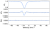 |
Fig. 1. Least-squares deconvolution profiles for the snapshot observations of HD 63433 with ESPaDOnS. The panels show the Stokes I (top), V (middle) and N (bottom) profiles, obtained from the combination of 4620 atomic spectral lines. We note the presence of a clear Zeeman signature in Stokes V, indicating that the large-scale magnetic field is amenable to characterisation. |
Our observations were carried out in circular polarisation mode only, considering the prohibitive exposure time required for linear polarisation mode for main sequence stars such as HD 63433. The inclusion of linear polarisation would allow us to reduce the cross-talk between the radial and meridional field components and obtain a better constrain of smaller magnetic field features (e.g. Rosén et al. 2015).
2.2. HARPSpol
HD 63433 was observed with HARPSpol4 (Snik et al. 2011; Piskunov et al. 2011), the spectropolarimeter for the HARPS spectrograph (Mayor et al. 2003) at the ESO 3.6 m telescope at La Silla observatory, Chile. The HARPSpol instrument is mounted at the Cassegrain focus of the telescope and has two polarimeters: for circular (Stokes V) and linear (Stokes QU) polarisation, respectively. Each polarimeter consists of a rotating retarder wave plate (a quarter-wave plate for the circular polarimeter and a half-wave plate for the linear polarimeter) and a beam-splitter – in this case a Foster prism – which splits the light into two beams with opposite polarisation states. These two beams are then fed via fibers to the HARPS spectrograph. Our HARPSpol observations cover the wavelength range between 380 and and 691 nm with a 8 nm gap at 529 nm separating the red and blue detectors. The spectral resolution is R = δλ/λ ≈ 110 000. We obtained circular polarisation observations on three separate nights: 22 December 2022, 24 December 2022, and 6 February 2023.
To reduce the HARPSpol data, we used the PyReduce package5 (Piskunov et al. 2021), the updated implementation in python of the versatile REDUCE package (Piskunov & Valenti 2002). The reduction with PyReduce is run with a series of standard steps, similar to REDUCE as described, for instance, Rusomarov et al. (2013). First, the mean of both bias and flat frames is computed, followed by the substraction of the mean bias from the mean flat. The final mean flat frame is then used to compute the normalized flat field, and to determine the location and shape of the spectral orders on the detectors. Science frames first get the bias subtracted and are divided by the normalized flat field to correct pixel-to-pixel variation in sensitivity. Scattered light is then subtracted from the science frames. Finally, the spectra from the two polarisation channels are extracted for each science frame. At this point, the extracted science spectra are in pixel space. To convert from pixel to wavelength space, we constructed a 2D wavelength solution from the wavelength calibration frames taken with the Thorium-Argon (ThAr) lamp as part of the regular daily calibrations. In this reduction, the blue and red detectors of HARPS are reduced independently.
We then applied LSD to the collected HARPSpol spectra using the same mask as ESPaDOnS. Compared to ESPaDOnS, the final LSD profiles are expected to be penalised due to the narrower spectral coverage of HARPSpol. For the night of 22 December 2022, we detected a Zeeman signature with FAP 8.7 × 10⁻⁹, and the Stokes V S/N is 7900. The two other nights do not show detections (FAP is 9.4 × 10⁻¹ and 3.8 × 10⁻²) and they correspond to the observations with the lowest S/N (see Table 2). Therefore, while we computed the longitudinal field only for the first observation, we measured the chromospheric activity indices for all three observations. Given that the spectral coverage of HARPSpol stops at 691 nm, we did not compute the Ca II infrared triplet activity diagnostics (see Sect. 3).
2.3. Neo-Narval
HD 63433 was observed by Neo-Narval6 between March and May 2023. We obtained six observations and although the phase coverage is not ideal, it is sufficient to reconstruct the topology of the large-scale magnetic field. The complete time series is summarised in Table 2. Neo-Narval is an upgrade to the Narval instrument at Télescope Bernard Lyot (Pic du Midi Observatory, Aurière 2003), operating between 370 and 1000 nm with a spectral resolving power of R = 65 000.
The Neo-Narval upgrade, implemented in 2019, included the installation of a new detector and improved velocimetric capabilities (López Ariste et al. 2022). Issues with the extraction of blue spectral orders occurred during the period of our observations (López Ariste et al. 2022), affecting especially those with very low S/N (below approximately 400 nm). As explained in the next section, this prevented us from studying Ca II H&K lines. In contrast, the computation of LSD profiles was less affected because LSD uses a S/N-weighting scheme. We adopted the same synthetic mask of 4620 lines as for ESPaDOnS and normalisation parameters, obtaining Stokes V profiles with the maximum S/N spanning between 7300 and 11 480. In the next sections, all the observations will be phased with the following ephemeris
 (1)
(1)
where we used the first Neo-Narval observation as JD reference, Prot is the stellar rotation period, and ncyc represents the rotation cycle (see Table 2).
3. Magnetic activity proxies
3.1. Activity indices
The spectral coverage of both ESPaDOnS, HARPSpol, and Neo-Narval encompasses chromospheric lines that are typically used to gauge chromospheric flux and thus assess stellar activity. As described in the next sections, we computed canonical activity indices using the Ca II H&K lines, the Hα line and Ca II infrared triplet lines. In the absence of star-planet interactions, these indices should vary at the stellar rotation period timescale (e.g. Mittag et al. 2017; Kumar & Fares 2023), although it is known that chromospheric complexity hampers rotation period measurements. For this reason, and considering the low number of observations, we did not perform a temporal analysis.
3.1.1. Ca II H&K index
Stellar activity has been quantified with the S index (Vaughan et al. 1978) and it was firstly adopted to search for activity cycles within the Mount Wilson project (Wilson 1968; Duncan et al. 1991). It is defined as the ratio between the flux of the Ca II H&K lines and the flux of the nearby continuum. Formally,
 (2)
(2)
where FH and FK are the fluxes in two triangular band passes with FWHM = 1.09 Å centred on the cores of the H line (3968.470 Å) and K line (3933.661 Å), whereas FR and FV are the fluxes within two 20-Å rectangular band passes centred at 3901 and 4001 Å, respectively. The set of coefficients {a, b, c, d, e} is used to convert the S-index from a specific instrument scale to the Mount Wilson scale. The coefficients for the ESPaDOnS instrument were estimated by Marsden et al. (2014), while for HARPSpol we used the optimisation of Boro Saikia et al. (2018). Given the Neo-Narval pipeline issue for the spectral region below 400 nm, we did not compute the activity index for the corresponding observations.
We determined the S-index from the intensity spectra of all four sub-exposures composing the ESPaDOnS snapshot observation (see Sect. 2), which we Doppler-shifted according to the radial velocity of the star (−15.9 km s−1). We found a mean value of 0.433 ± 0.021, where the error bar is obtained as standard deviation between the four sub-exposures divided by two (i.e. the square root of the number of sub-exposures). We took this approach since the measurement of an activity indicator for a particular night has the benefit of an increased S/N thanks to the combination of sub-exposures. The value of S-index remains consistent if computed directly from the intensity spectrum obtained as combination of the four sub-exposures. The S/N in the spectral region where the Ca II H&K lines lie is too low in the HARPSpol observations for a reliable measurement.
The S-index contains a colour dependence that biases the comparison of activity levels between stars, as well as a photospheric contribution in the line wings due to magnetic heating (Noyes et al. 1984). For this reason, the chromospheric activity index  is typically used (Middelkoop 1982; Noyes et al. 1984; Rutten 1984). The conversion yielded a value of −4.345 ± 0.027 for the ESPaDOnS observation.
The index values we estimated from the ESPaDOnS spectrum are consistent with the range for which large-scale magnetic fields of active cool dwarfs are detectable (Marsden et al. 2014). They are compatible within uncertainties with the range reported by Pace (2013) and Boro Saikia et al. (2018), but they are larger by 0.06 dex (3σ) than the individual measurement in 2010 computed by Marsden et al. (2014).
3.1.2. Hα index
We measured the flux of the Hα line normalised by the nearby continuum following Gizis et al. (2002). This line is formed in the upper chromosphere, thus providing insights into this particular region of the stellar atmosphere. Formally,
 (3)
(3)
where FHα is the flux within a rectangular band pass of 3.60 Å centred on the Hα line at 6562.85 Å, and HV and HR are the fluxes within two rectangular band passes of 2.2 Å centred on 6558.85 Å and 6567.30 Å (see Fig. 2).
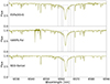 |
Fig. 2. Normalised fluxes around the Hα line for the three instruments used in this study. From the top: ESPaDOnS, HARPSpol, and Neo-Narval. The black rectangles indicate the regions used in the definition of the corresponding activity index. The observations were taken between September 2022 and May 2023. |
The temporal evolution of the values computed from Neo-Narval spectra is shown in Fig. 3 and the values are reported in Table 3. From the ESPaDOnS snapshot observation, we obtained a value of 0.341 ± 0.002, from HARPSpol we measured 0.339 ± 0.001, 0.339 ± 0.001, and 0.331 ± 0.002, and from Neo-Narval, we estimated values between 0.336 and 0.342 with a mean of 0.339 ± 0.002. Even though all observations spanned eight months in total, the activity level, as quantified by the Hα index, did not indicate a substantial evolution.
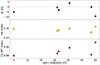 |
Fig. 3. Time series of longitudinal magnetic field and activity indices measurements for HD 63433 from the Neo-Narval observations. The longitudinal field (top panel) exhibits intermittency in the sign of the magnetic polarity, which is symbolic of a likely complex or non-axisymmetric topology. The Hα index (middle panel) does not exhibit strong variations, while the Ca II IRT index (bottom panel) has an increased scatter towards the latest observations. The Hα and Ca II IRT indices show correlated temporal evolution. |
Activity indices and longitudinal magnetic field measurements.
3.1.3. Ca II infrared triplet index
Another chromospheric activity indicator is the Ca II infrared-triplet (IRT) index, which is a diagnostic for the lower chromosphere (Montes et al. 2000; Hintz et al. 2019). We followed Petit et al. (2013) and Marsden et al. (2014), computing:
 (4)
(4)
where IR1, IR2, and IR3 are the fluxes within a rectangular band pass of 2 Å centred on the Ca II lines at 8498.023, 8542.091, and 8662.410 Å, respectively, and IRR and IRV are the fluxes within two rectangular band passes of 5 Å centred on 8704.9 Å and 8475.8 Å. The spectral coverage of HARPSpol does not encompass these calcium lines; hence, we did not compute the index for the corresponding observations.
The temporal evolution is shown in Fig. 3 and the values reported in Table 3. From the ESPaDOnS snapshot observation, we obtained a value of 0.899 ± 0.002, whereas from the Neo-Narval observations, we estimated values between 0.880 and 0.910 with a mean of 0.891 ± 0.002. In a similar manner to Hα index, the magnetic activity level seems to have remained reasonably stable, with the oscillations due to intrinsic variability of active regions. In general, we caution that robust conclusions on the evolution of the activity level based on the activity proxies computed here cannot be drawn, considering the large gaps between observations as well as the low number of observations.
3.2. Longitudinal magnetic field
We computed the disk-integrated, line-of-sight-projected component of the large-scale magnetic field following Donati et al. (1997) for the snapshot ESPaDOnS observation, the first HARPSpol observation, and the six Neo-Narval observations. We used the general formula as in Cotton et al. (2019),
 (5)
(5)
where λ0 and geff are the normalisation wavelength and Landé factor of the LSD profiles, Ic is the continuum level, v is the radial velocity associated to a point in the spectral line profile in the star’s rest frame, h is the Planck’s constant, and μB is the Bohr magneton. To express it as in Rees & Semel (1979) and Donati et al. (1997), it is possible to use hc/μB = 0.0214 Tm, where c is the speed of light in m s−1.
The computation was carried out within ±20 km s−1 from line centre at −15.9 km s−1 for both Stokes I and V. We found a value of 3.2 ± 0.9 G for the ESPaDOnS snapshot observation, 6.4 ± 2.0 G for the HARPSpol observation and a range between −9.4 and 3.6 G for the Neo-Narval observations. The median formal error bar is 2.0 G. In comparison, the value reported in 2010 by Marsden et al. (2014) is 2.5 ± 0.5 G. We illustrate the time series of Bl measurements in Fig. 3. The fast-changing sign is symbolic of a complex magnetic field topology, which is expected for stars of similar properties to HD 63433 (e.g. Morgenthaler et al. 2012; Strassmeier et al. 2023).
3.3. Correlations of activity proxies
We inspected the correlations between |Bl|, the Hα index and the Ca II IRT index for the six Neo-Narval observations. The results are given in Fig. 4. In general, we caution that these correlations are found with a statistically low number of observations. Therefore, our main aim is to check that we see the expected trends, even for a low number of observations.
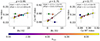 |
Fig. 4. Correlation plots for the activity proxies computed from the six Neo-Narval observations. From the left: Hα vs. |Bl|, Ca II IRT vs. |Bl|, and Hα vs. Ca II IRT. Each data point is colour-coded based on the rotational cycle as computed from Eq. (1). Each panel displays the Pearson correlation coefficient (ρ) at the top and a linear fit as black dashed line. The green cross indicates the values of the ESPaDOnS snapshot observation, but it was not included in the computation of the Pearson correlation coefficient. We included the first HARPSpol observation in the first panel as a blue cross. |
The activity indices are computed from unpolarised spectra, which are sensitive to both small and large spatial scales and, thus, to most magnetic features. Instead, the longitudinal field is derived from circularly polarised spectra, which are known to be sensitive to large-scales only, owing to polarity cancellation effects. For this reason, moderate correlations or more complex behaviours between these quantities have been reported for cool dwarfs (Petit et al. 2008; Morgenthaler et al. 2012; Marsden et al. 2014; Boro Saikia et al. 2016; Brown et al. 2022).
Here, we obtained a strong positive correlation between Hα index and |Bl| of Pearson correlation coefficient ρ = 0.95. The ESPaDOnS and HARPSpol values are not included in the computation of ρ, because the corresponding observations were collected months before (see Table 3), hence intrinsic variability may have occurred (the inclusion of these two points yields ρ = 0.79, as expected from a loss of coherency of activity over long timescales). For the Ca II IRT index versus |Bl| case and the Hα versus Ca II IRT index case, we obtained ρ = 0.75 and 0.77, respectively. While still strong, the lower level of correlation is likely due to the different chromospheric regions that Hα index and Ca II IRT index probe (see e.g. Hintz et al. 2019). Figure 4 also demonstrates the high variability of magnetic activity for this star, since the last two measurements (yellow circles beyond rotational cycle 8.0) are at the extremes of the measurements range of the indices (see also Table 3).
4. Zeeman-Doppler imaging
We applied ZDI on the six Neo-Narval observations to map the large-scale magnetic field at the surface of HD 63433. Formally, the field is expressed as the sum of a poloidal and toroidal component, and both components are described by means of spherical harmonic decomposition (Donati et al. 2006; Lehmann & Donati 2022). The ZDI algorithm generates a time series of Stokes V profiles and adjusts them to the observations iteratively until a target  is reached. The goal is to fit the spherical harmonics coefficients αℓ, m, βℓ, m, and γℓ, m (with ℓ and m being the degree and order of the mode, respectively). The algorithm adopts a maximum-entropy regularisation scheme to reconstruct the magnetic field configuration compatible with the data and with the lowest information content (for more information see Skilling & Bryan 1984; Donati et al. 1992, 1997). In practice, we employed the python zdipy code described in Folsom et al. (2018)7, assuming weak-field approximation (see e.g. Landi Degl’Innocenti 1992).
We adopted the following stellar input parameters (Mann et al. 2020): inclination of 70°, projected equatorial velocity (veq sin i) of 7.3 km s−1, rotation period of 6.45 d, and solid body rotation. The value of veq sin(i) is consistent with other dedicated studies (Rainer et al. 2023). We set a linear limb darkening coefficient of 0.7 (Claret & Bloemen 2011) and the maximum degree of harmonic expansion ℓmax = 5, consistently with the spatial resolution allowed by veq sin(i). Using larger values of ℓmax did not improve the fit since the magnetic energy is stored only in the modes up to ℓ = 5.
The time series of Neo-Narval Stokes V profiles is shown in Fig. 5. The shape of the LSD profiles suggests that the field topology includes a significant contribution from the toroidal component. The last observation at cycle 9.30 seems to have a more antisymmetric shape, which is typical of a more dipolar configuration instead (Morin et al. 2008a,b; Bellotti et al. 2023a,b). Such variation in profile shape is likely due to stellar rotation rather than intrinsic evolution, considering the short phase separation with the previous observations. As a result, we expect a magnetic feature of negative polarity in the radial field at that phase.
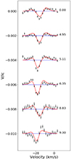 |
Fig. 5. Time series of circularly polarised Stokes profiles obtained with Neo-Narval. Observations are shown as black dots and ZDI models as red lines and they are offset vertically for better visualisation. The number on the right is the rotational cycle (see Eq. (1)). |
A qualitative assessment of the axisymmetric component of the magnetic field can be obtained by decomposing the median Stokes V profile into its symmetric and asymmetric components (Lehmann & Donati 2022). We show this exercise in Fig. 6, where we see that the median Stokes V shape is mostly symmetric, suggesting a significant contribution from the toroidal component of the field. In parallel, the antisymmetric shape exhibits a strong signal, meaning that the poloidal component is also contributing substantially to the profile shape. From this, one can expect the axisymmetric component of the field to be mostly toroidal (in agreement with Petit et al. 2008), but with a substantial poloidal contribution as well. This confirms the capability of the symmetric-antisymmetric decomposition to qualitatively determine the main magnetic field component. This could be particularly useful when a large number of stars have to be analysed before a detailed ZDI analysis is carried out.
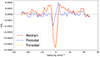 |
Fig. 6. Decomposition of the median Stokes V LSD profile into its symmetric and antisymmetric components. We note that the median Stokes V (red line) has mostly a symmetric shape (yellow line) which indicates a strong toroidal component. At the same time, there is still a significant contribution from the antisymmetric shape (blue line), namely, the poloidal component. |
The Stokes V profiles were fit down to  = 1.2, from an initial value of 6.5 (see Fig. 5). The value was chosen to prevent artificial injection of magnetic energy in high order modes or reconstruction of substantially weak fields, which would be symbolic of overfitting and underfitting of the Stokes V profiles, respectively (see e.g. Alvarado-Gómez et al. 2015). Lowering the
  further would likely require the inclusion of differential rotation as intrinsic variability mechanism, but with our sparse observations it cannot be constrained.
The properties of the magnetic map are given in Table 4 and the map is shown in Fig. 7. The mean magnetic field strength is Bmean = 24 G, with the toroidal component accounting for 54% of the magnetic energy and the poloidal component for 46%. The dipolar mode accounts for 30% of the poloidal energy and both the quadrupolar and quadrupolar modes store a significant fraction, namely, 26% and 15%.
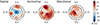 |
Fig. 7. ZDI reconstruction in flattened polar view of the large-scale field of HD 63433. From the left, the radial, azimuthal, and meridional components of the magnetic field vector are illustrated. The radial ticks are located at the rotational phases when the observations were collected, while the concentric circles represent different stellar latitudes: −30°, +30°, and +60° (dashed lines), as well as the equator (solid line). The geometry is complex, with a significant toroidal fraction and the poloidal component distributed mainly in the dipolar, quadrupolar, and octupolar modes. The colour bar encapsulates the magnetic field strength, up to a maximum of 55 G. |
Properties of the magnetic map.
To set the uncertainties on the magnetic field properties, we estimated variation bars following Mengel et al. (2016), Fares et al. (2017), and Bellotti et al. (2023a). The idea is to vary the input parameters, namely inclination, veq sin(i), and rotation period to plausible values consistent with the literature. One at a time, we set these input parameters to the extremes of the range of values reported in the literature, and reconstructed the corresponding map of the magnetic field. The variation bars on the field characteristics are then the maximum deviations of these new maps from the reconstruction with the optimised parameters. These variation bars do not capture the actual error bars, but, rather, the sensitivity of the reconstructed properties to input parameters.
Quantitatively, Mann et al. (2020) constrained the stellar inclination to be larger than 74°; hence, we reconstructed maps with i = 60° and i = 80°. For veq sin i, we used 6.5 km s−1 and 7.9 km s−1 (Damasso et al. 2023) and for Prot we used 6.0 d (Mallorquín et al. 2023) and 7.6 d (Marsden et al. 2014). We adopted a target  of 1.2 in every case, except for Prot = 6.0 d for which we used
  = 2.4. This already indicates that using such value of rotation period degrades significantly the magnetic field model. The variation bars of the magnetic characteristics are driven predominantly by the uncertainties on the rotation period, since the variations in inclination and veq sin i have led to magnetic maps that are reasonably consistent with the reconstruction when using the optimised parameters.
To check the robustness of our results, we reconstructed a map excluding the last observation. The only change is in the energy fraction in the poloidal component, as it decreases to 25%. This is not surprising considering that the shape of Stokes V in the last spectropolarimetric observation is the most similar to a typical poloidal-dipolar field (e.g. Morin et al. 2008a; Bellotti et al. 2023a). The average field strength changes only by 1 G, while the dipolar, quadrupolar and octupolar energy fraction by less than 2% and the axisymmetric fraction by less than 15%. Such changes are encompassed by the variation bars we estimated in this work.
5. ZDI-driven stellar wind models
We created the stellar wind models using the Alfvén wave solar model (AWSoM, Sokolov et al. 2013; van der Holst et al. 2014), which is a component in the Space Weather Modelling Framework (SWMF, Tóth et al. 2005, 2012). This model solves the ideal two-temperature magnetohydrodynamic equations, supplemented by a pair of equations describing the propagation of Alfvén wave energy along magnetic field lines. The model extends from the chromosphere, where the temperature is 5 × 10⁴ K and the density is 2 × 10¹⁷ m3, through the transition region to the stellar corona. The model is driven by the energy flux of Alfvén waves, which crosses the inner boundary at a rate proportional to the local magnetic field strength at the stellar surface. The Poynting flux-to-field ratio is set to 1.1 × 10⁶ W m−2 T−1 and the turbulence correlation length is 1.5 × 10⁵ m T1/2. The radial component of the surface magnetic field is held to the Br values in Fig. 7, while the transverse components are left to evolve with the numerical solution. The AWSoM model was configured using solar values that have been shown to reproduce solar conditions (Meng et al. 2015; van der Holst et al. 2019; Sachdeva et al. 2019). The coronal heating due to Alfvén waves is likely to resemble that of the Sun, according to the non-thermal velocity measurements of sun-like stars of similar rotation periods in Boro Saikia et al. (2023). For a more detailed description of the methodology behind the wind models, we refer to Evensberget et al. (2021, 2022, 2023).
The top panel of Fig. 8 shows the stellar magnetic field embeded in the stellar wind equator-on. The large scale coronal magnetic field resembles a dipole with closed regions pushed towards the positive z axis. We also see arch-like structures where the magnetic field lines connect regions of opposite polarity, which are the result of quadrupolar and octupolar components of the magnetic field as may be seen also in the radial field plot of Fig. 7. In our model, the wind mass loss rate is 1.1 × 10⁻¹³ M⊙ yr−1, which is about five times the solar wind mass loss rate.
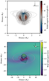 |
Fig. 8. Simulated environment of HD 63433. Top: steady-state coronal magnetic field structure obtained from our ZDI-driven stellar wind model. Open magnetic field lines are truncated at two stellar radii, while the closed field lines are not truncated. The star is seen equator on at the rotational phase 0.35. The large-scale structure exhibits a mostly dipolar topology. The colours are the same as Fig. 7. Bottom: Alfvén surface and wind radial speed. The two-lobed Alfvén surface is characteristic for a dipole-dominated coronal magnetic field. The intersection of the Alfvén surface and the stellar equatorial plane is shown as a white curve, while the the planetary orbits are shown in orange, red, and pink. The orbital plane is colour-coded by the wind radial speed. |
The bottom panel of Fig. 8 shows the Alfvén surface, where the stellar wind speed equals the Alfvén wave velocity. This quantity is crucial to understand the regime in which magnetic or inertial forces dominate, within or outside the surface, respectively (e.g. Vidotto 2021). A practical quantity in this context is the Alfvén Mach number, which is defined as the ratio of the wind speed, vsw, to the Alfvén wave speed of  , where B is the local magnetic field strength and ρsw is the local wind density. The Alfvén Mach number quantifies whether the planetary motion is super-(MA > 1) or sub-Alfvénic (MA < 1). The Alfvén surface corresponds to MA = 1.
The orbits of planet d, b, and c are shown in the bottom panel of Fig. 8 as concentric curves at 9.9, 16.8, and 36.1 R⋆ (Damasso et al. 2023; Mallorquín et al. 2023; Capistrant et al. 2024). For the three planets, we assume that the planets have circular orbits in the equatorial plane of the star, consistently with the literature estimates within error bars (Mann et al. 2020; Damasso et al. 2023; Capistrant et al. 2024). The orbit of the innermost planet in our model crosses briefly the Alfvén surface into the sub-Alfvénic regime; we discuss it further in Sect. 6.
Figure 9 shows the wind speed vsw, density, ρsw, and wind ram pressure,  , in the planetary frame, as a function of stellar rotation phase. We note the presence of three dips in the wind speed curves. These are correlated to the three arms of the wind spiral shape which, in turn, are due to stellar rotation (see Fig. 8). Such spiral features were already reported, and tend to build more arms if the field complexity is larger (Evensberget et al. 2021). The wind density experienced by each planet can vary by a factor of ∼5 along planetary orbits. For the ram pressure, the variation is somewhat smaller than that of the density.
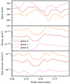 |
Fig. 9. Stellar wind conditions in the planetary frame. From the top: wind speed, density, and ram pressure are shown as a function of stellar rotation phase. Planets b, c, and d are colour-coded in red, pink, and orange. |
Figure 10 shows the Alfvén Mach number (MA) computed in the planetary frame as a function of stellar rotational phase. In our model, we see that planet d experiences sub-Alfvénic winds at stellar rotation phases 0.38−0.50, whereas planets b and c orbit in super-Alfvénic motions. In the next section, we discuss what these locations translate to in terms of star-planet interactions and their observable signatures.
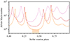 |
Fig. 10. Alfvén Mach number computed in the planetary frame as a function of stellar rotation phase. The colours and labels are the same as in Fig. 9. The phase interval where our model’s planet d crosses into the sub-Alfvénic regime is shown as a green shaded region. |
6. Summary and discussion
We have characterised the magnetic field and environment of the active, young G5 dwarf star HD 63433, which is known to host two sub-Neptunes and an Earth-sized planet. We computed magnetic activity diagnostics such as the chromospheric S index,  , Hα, Ca II infrared triplet, and longitudinal magnetic field, using observations from ESPaDOnS, HARPSpol, and Neo-Narval. We then reconstructed the large-scale magnetic field by means of ZDI and used it as boundary condition for the simulation of the system’s stellar wind from the corona to the orbital distances of the planets b, c, and d, following the method presented in Evensberget et al. (2021). In general, the observations and analyses were conducted as part of a survey dedicated to the spectropolarimetric characterisation of bright stars in the current list of potential Ariel targets, in order to efficiently construct the final target list before the launch and, consequently, optimize the science outcome of the mission.
We estimated S = 0.433 ± 0.041 and  = −4.345±0.055, which are compatible with the measurements of other Sun-like stars with analogous spectral type, mass, rotation period, and age (ξ Boo A, Morgenthaler et al. 2012; Strassmeier et al. 2023; HD 1237, Alvarado-Gómez et al. 2015; HD 147513, Hussain et al. 2016; κ Cet, do Nascimento et al. 2016). In comparison, the average values for the Sun at cycle maxima and minima are
  = −4.905 and −4.984 (Egeland et al. 2017).
The longitudinal magnetic field of HD 63433 varies between −11 and 5 G, which is typical for solar-like stars. For instance, Morgenthaler et al. (2012) found variations between −2.3 and 22 G for ξ Boo A, Boro Saikia et al. (2016) reported values spanning −20 and 10 G across different epochs of HN Peg, and Alvarado-Gómez et al. (2015) reported a range between −10 and 10 G for HD 1237. The large-scale field is three times stronger (in absolute value) than the Sun, whose large-scale field values can reach 3−4 G (Kotov et al. 1998).
The reconstructed magnetic field topology of HD 63433 is complex, with a significant amount of energy stored in the toroidal and poloidal components (see Sect. 3). The average field strength in absolute value is around 23 G. This is of the same order of magnitude as estimated by Zhang et al. (2022) who employed the age-magnetic field strength law of Vidotto et al. (2014) to include the effects of stellar magnetic fields in the outflow models of planet b and c. In our model, the derived stellar wind mass loss rate is 1.1 × 10⁻¹³ M⊙ yr−1, which is 2.9 times smaller than the value derived from the simulations of Zhang et al. (2022). The stellar wind can affect atmospheric escape in exoplanets in several ways, from potentially reducing escape rates (Vidotto & Cleary 2020) and altering the signatures of atmospheric evaporation through spectroscopic transits (Carolan et al. 2021), even to possibly creating a tenuous atmosphere through sputtering processes (Vidotto et al. 2018). Recently, Zhang et al. (2022) modelled the escaping atmospheres of HD 63433 b and c, including the effects of the interaction with the stellar wind. So far, no model exists for the escaping atmosphere of the recently discovered innermost planet HD 63433 d. With the optimally constrained stellar wind properties presented in our work, future atmospheric models of HD 63433 d will be able to better pin-point the effects of the wind of the host star on the upper atmosphere of HD 63433 d, as well as potential signatures in Ly-α and He I transits. Such models are important to assess the presence and evolution of the atmosphere of HD 63433 d (Kubyshkina et al. 2022).
Finally, we illustrate the properties of the field geometry of HD 63433 compared to other stars in Fig. 11. Although the number of observations used for tomographic inversion is limited, the magnetic field exhibits similarities with other Sun-like stars of similar properties and remarkably with the field map of ξ Boo A from 2008 (Morgenthaler et al. 2012) because it also exhibits a dominating polarity at the north pole, as well as lower latitude magnetic spots.
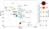 |
Fig. 11. Properties of the magnetic topologies for cool, main sequence stars obtained via ZDI. The location of HD 63433 is highlighted. The y- and x-axes represent the mass and rotation period of the star, and iso-Rossby number curves are overplotted using the empirical relations of Wright et al. (2018). The symbol size, colour and shape encodes the ZDI average field strength, the poloidal and toroidal energy fraction, and axisymmetry. Data entering the plot are taken from Petit et al. (2008), Morgenthaler et al. (2012), Fares et al. (2013), Boro Saikia et al. (2015, 2016), do Nascimento et al. (2016), Hussain et al. (2016), Alvarado-Gómez et al. (2015), Folsom et al. (2016, 2018, 2020), Klein et al. (2021), Willamo et al. (2022), Martioli et al. (2022). |
In terms of evolution, Maldonado et al. (2022) analysed activity indices and photometric light curves of HD 63433, and estimated the lifetime of active regions to be approximately 60 d. Additionally, Lehtinen et al. (2016) reported cyclic photometric variability on a 2.7 yr timescale and a less significant variation of approximately 8.0 yr. If we maintain the analogy with ξ Boo A, Morgenthaler et al. (2012) reported fast variations over timescales of six months of the field topology and complexity, from a poloidal-dominated to a toroidal-dominated regime. Overall, this shows that HD 63433 could manifest evident and important variability, which motivates additional spectropolarimetric monitoring.
From the stellar environment simulations, we obtained a largely dipolar coronal magnetic field, aligned with the stellar axis of rotation. We also see arch-like structures where the magnetic field lines connect regions of opposite polarity, resulting from the quadrupolar and octupolar components of the magnetic field. Using our wind model, we computed the location of the Alfvén surface where the wind speed equals the Alfvén wave velocity. The Alfvén surface is two-lobed, which is characteristic for a dipole-dominated coronal magnetic field.
We found that the outermost two planets orbit in the super-Alfvénic region. In this regime, a bow shock between the stellar wind and a planetary magnetosphere (if present) can be generated and the stellar wind is deflected around the planet (Chapman & Ferraro 1931; Vidotto et al. 2009, 2010). Also, the formation of a tail-like structure of evaporated planetary material can occur (e.g. Schneiter et al. 2007; Villarreal D’Angelo et al. 2018; Zhang et al. 2022). Star-planet interactions in super-Alfvénic regime are expected to produce auroral radio emission from the planetary magnetosphere, similarly to Solar System planets (Zarka et al. 2001).
The innermost Earth-sized planet is located in the trans-Alfvénic region, as our modelling indicates that the stellar wind conditions along its orbit may switch between sub- and super-Alfvénic. Within the sub-Alfvénic regime, the planet can directly link to the stellar magnetic field, and its motion can perturb the field lines producing Alfvén waves travelling starward; alternatively, it can induce magnetic reconnection events (if magnetised) or a combination of both (e.g. Neubauer 1998; Ip et al. 2004; Strugarek et al. 2015; Kavanagh et al. 2022). In turn, these phenomena generate detectable signatures such as coronal radio emission on the star (Saur et al. 2013; Kavanagh et al. 2021) and local chromospheric flux enhancement (Shkolnik et al. 2008; Lanza 2009).
We note that the magnetic field strength recovered from ZDI could be underestimated (Lehmann et al. 2019). On one side, the latitudinal coverage of the star is limited by definition, as we can only model the disk intersected by the line of sight. On the other side, the low number of observations combined with the poor longitudinal coverage of the stellar rotation may prevent us from reconstructing additional large-scale magnetic features. For these reasons, a more robust wind model will be provided in the future with an updated map built from a denser spectropolarimetric monitoring. Although spectropolarimetric time series with a scarce sampling may limit the reconstruction of the large-scale magnetic topology, the first-order information that we can derive from them is still relevant feedback for Ariel target planning. They allow us to assess the magnetic activity level of the star and its variation over distinct timescales: from rotational modulation to long-term evolution, potentially in the form of a magnetic cycle, which could be seen as a magnetic polarity reversal even from multiple epochs in which the rotational phase coverage is not optimal (see Fig. 1 Boro Saikia et al. 2016, for example).
This work has been developed within the science development of the ESA Ariel space mission, for which more magnetic activity characterisation studies will be presented in the upcoming future. It represents the start of a campaign dedicated to the magnetic characterisation of stars in the current list of Ariel targets (Edwards & Tinetti 2022). In this regard, additional observations of HD 63433 are necessary to understand the long-term evolution of its large scale magnetic field. This will be also valuable to our understanding of the observational signatures of star-planet interactions due to the correlated long-term evolution of the Alfvén surface. Indeed, it would be interesting to observe the star along its likely magnetic cycle to characterize how the Alfvén surface moves with respect to the planetary orbits. Observations in the UV range will also be essential, as X-ray observations show a difference of around two orders of magnitude between the Sun and HD 63433. This raises the question of how the UV wavelength range differs and the consequences on the atmospheric photochemistry, heating, and loss. Ultimately, this information can provide practical constraints for the observing strategies of Ariel, for such targets as the HD 63433 system. Once the mission is launched, the goal of our spectropolarimetric campaign will become more of a follow-up work, aimed at complementing the observations already performed and providing new insights for the interpretation of Ariel data.
www.exoplanet.eu, December 2023.
Available at https://github.com/folsomcp/ZDIpy
Acknowledgments
This publication is part of the project “Exo-space weather and contemporaneous signatures of star-planet interactions” (with project number OCENW.M.22.215 of the research programme “Open Competition Domain Science-M”), which is financed by the Dutch Research Council (NWO). This work used the Dutch national e-infrastructure with the support of the SURF Cooperative using grant nos. EINF-2218 and EINF-5173. S.B. acknowledges funding from the SCI-S department of the European Space Agency (ESA), under the Science Faculty Research fund E/0429-03. A.A.V. and D.E. acknowledge funding from the European Research Council (ERC) under the European Union’s Horizon 2020 research and innovation programme (grant agreement No. 817540, ASTROFLOW). S.B.S. was supported by the Austrian Science Fund (FWF) Lise Meitner grant M2829-N. C.D. acknowledges financial support from the INAF initiative “IAF Astronomy Fellowships in Italy”, grant name GExoLife. G.M. acknowledges the support of the ASI-INAF agreement 2021-5-HH.0 and PRIN MUR 2022 (project No. 2022J7ZFRA, EXO-CASH). Based on observations obtained at the Canada-France-Hawaii Telescope (CFHT) which is operated by the National Research Council of Canada, the Institut National des Sciences de l’Univers of the Centre National de la Recherche Scientique of France, and the University of Hawaii. Based on observations collected at the European Southern Observatory under ESO programme 110.24C8.002 (P.I. S. Bellotti). We thank the TBL team for providing service observing with Neo-Narval. This work has made use of the VALD database, operated at Uppsala University, the Institute of Astronomy RAS in Moscow, and the University of Vienna; Astropy, 12 a community-developed core Python package for Astronomy (Astropy Collaboration 2013, 2018); NumPy (van der Walt et al. 2011); Matplotlib: Visualization with Python (Hunter 2007); SciPy (Virtanen et al. 2020) and PyAstronomy (Czesla et al. 2019).
References
- Airapetian, V. S., Glocer, A., Khazanov, G. V., et al. 2017, ApJ, 836, L3 [NASA ADS] [CrossRef] [Google Scholar]
- Allan, A., & Vidotto, A. A. 2019, MNRAS, 490, 3760 [Google Scholar]
- Alvarado-Gómez, J. D., Hussain, G. A. J., Grunhut, J., et al. 2015, A&A, 582, A38 [NASA ADS] [CrossRef] [EDP Sciences] [Google Scholar]
- Astropy Collaboration (Robitaille, T. P., et al.) 2013, A&A, 558, A33 [NASA ADS] [CrossRef] [EDP Sciences] [Google Scholar]
- Astropy Collaboration (Price-Whelan, A. M., et al.) 2018, AJ, 156, 123 [Google Scholar]
- Aurière, M. 2003, in EAS Publications Series, eds. J. Arnaud, & N. Meunier, 9, 105 [CrossRef] [EDP Sciences] [Google Scholar]
- Bagnulo, S., Landolfi, M., Landstreet, J. D., et al. 2009, PASP, 121, 993 [Google Scholar]
- Bellotti, S., Fares, R., Vidotto, A. A., et al. 2023a, A&A, 676, A139 [NASA ADS] [CrossRef] [EDP Sciences] [Google Scholar]
- Bellotti, S., Morin, J., Lehmann, L. T., et al. 2023b, A&A, 676, A56 [NASA ADS] [CrossRef] [EDP Sciences] [Google Scholar]
- Boro Saikia, S., Jeffers, S. V., Petit, P., et al. 2015, A&A, 573, A17 [NASA ADS] [CrossRef] [EDP Sciences] [Google Scholar]
- Boro Saikia, S., Jeffers, S. V., Morin, J., et al. 2016, A&A, 594, A29 [NASA ADS] [CrossRef] [EDP Sciences] [Google Scholar]
- Boro Saikia, S., Lueftinger, T., Jeffers, S. V., et al. 2018, A&A, 620, L11 [NASA ADS] [CrossRef] [EDP Sciences] [Google Scholar]
- Boro Saikia, S., Lueftinger, T., Airapetian, V. S., et al. 2023, ApJ, 950, 124 [NASA ADS] [CrossRef] [Google Scholar]
- Brown, E. L., Jeffers, S. V., Marsden, S. C., et al. 2022, MNRAS, 514, 4300 [CrossRef] [Google Scholar]
- Capistrant, B. K., Soares-Furtado, M., Vanderburg, A., et al. 2024, AJ, 167, 54 [NASA ADS] [CrossRef] [Google Scholar]
- Carmona, A., Delfosse, X., Bellotti, S., et al. 2023, A&A, 674, A110 [NASA ADS] [CrossRef] [EDP Sciences] [Google Scholar]
- Carolan, S., Vidotto, A. A., Villarreal D’Angelo, C., & Hazra, G. 2021, MNRAS, 500, 3382 [Google Scholar]
- Changeat, Q., Keyte, L., Waldmann, I. P., & Tinetti, G. 2020, ApJ, 896, 107 [NASA ADS] [CrossRef] [Google Scholar]
- Chapman, S., & Ferraro, V. C. A. 1931, J. Geophys. Res., 36, 77 [Google Scholar]
- Chavez, E., de Pater, I., Redwing, E., et al. 2023, Icarus, 404, 115667 [NASA ADS] [CrossRef] [Google Scholar]
- Claret, A., & Bloemen, S. 2011, A&A, 529, A75 [NASA ADS] [CrossRef] [EDP Sciences] [Google Scholar]
- Cotton, D. V., Evensberget, D., Marsden, S. C., et al. 2019, MNRAS, 483, 1574 [NASA ADS] [CrossRef] [Google Scholar]
- Cracchiolo, G., Micela, G., & Peres, G. 2021, MNRAS, 501, 1733 [Google Scholar]
- Czesla, S., Schröter, S., Schneider, C. P., et al. 2019, Astrophysics Source Code Library [record ascl:1906.010] [Google Scholar]
- Damasso, M., Locci, D., Benatti, S., et al. 2023, A&A, 672, A126 [NASA ADS] [CrossRef] [EDP Sciences] [Google Scholar]
- Danielski, C., Brucalassi, A., Benatti, S., et al. 2022, Exp. Astron., 53, 473 [NASA ADS] [CrossRef] [Google Scholar]
- Di Maio, C., Changeat, Q., Benatti, S., & Micela, G. 2023, A&A, 669, A150 [NASA ADS] [CrossRef] [EDP Sciences] [Google Scholar]
- do Nascimento, J. D., Vidotto, A. A., Petit, P., et al. 2016, ApJ, 820, L15 [NASA ADS] [CrossRef] [Google Scholar]
- Donati, J. F. 2003, in Solar Polarization, eds. J. Trujillo-Bueno, & J. Sanchez Almeida, ASP Conf. Ser., 307, 41 [Google Scholar]
- Donati, J. F., Brown, S. F., Semel, M., et al. 1992, A&A, 265, 682 [Google Scholar]
- Donati, J. F., Semel, M., Carter, B. D., Rees, D. E., & Collier Cameron, A. 1997, MNRAS, 291, 658 [Google Scholar]
- Donati, J.-F., Forveille, T., Collier Cameron, A., et al. 2006, Science, 311, 633 [Google Scholar]
- Dumusque, X., Udry, S., Lovis, C., Santos, N. C., & Monteiro, M. J. P. F. G. 2011, A&A, 525, A140 [NASA ADS] [CrossRef] [EDP Sciences] [Google Scholar]
- Duncan, D. K., Vaughan, A. H., Wilson, O. C., et al. 1991, ApJS, 76, 383 [Google Scholar]
- Edwards, B., & Tinetti, G. 2022, AJ, 164, 15 [NASA ADS] [CrossRef] [Google Scholar]
- Edwards, B., Mugnai, L., Tinetti, G., Pascale, E., & Sarkar, S. 2019, AJ, 157, 242 [NASA ADS] [CrossRef] [Google Scholar]
- Egeland, R., Soon, W., Baliunas, S., et al. 2017, ApJ, 835, 25 [NASA ADS] [CrossRef] [Google Scholar]
- Evensberget, D., Carter, B. D., Marsden, S. C., Brookshaw, L., & Folsom, C. P. 2021, MNRAS, 506, 2309 [NASA ADS] [CrossRef] [Google Scholar]
- Evensberget, D., Carter, B. D., Marsden, S. C., et al. 2022, MNRAS, 510, 5226 [NASA ADS] [CrossRef] [Google Scholar]
- Evensberget, D., Marsden, S. C., Carter, B. D., et al. 2023, MNRAS, 524, 2042 [CrossRef] [Google Scholar]
- Fares, R., Moutou, C., Donati, J. F., et al. 2013, MNRAS, 435, 1451 [NASA ADS] [CrossRef] [Google Scholar]
- Fares, R., Bourrier, V., Vidotto, A. A., et al. 2017, MNRAS, 471, 1246 [Google Scholar]
- Folsom, C. P., Petit, P., Bouvier, J., et al. 2016, MNRAS, 457, 580 [Google Scholar]
- Folsom, C. P., Bouvier, J., Petit, P., et al. 2018, MNRAS, 474, 4956 [NASA ADS] [CrossRef] [Google Scholar]
- Folsom, C. P., Ó Fionnagáin, D., Fossati, L., et al. 2020, A&A, 633, A48 [NASA ADS] [CrossRef] [EDP Sciences] [Google Scholar]
- Gagné, J., Mamajek, E. E., Malo, L., et al. 2018, ApJ, 856, 23 [Google Scholar]
- Gaia Collaboration 2020, VizieR Online Data Catalog: I/350 [Google Scholar]
- Gardner, J. P., Mather, J. C., Clampin, M., et al. 2006, Space Sci. Rev., 123, 485 [Google Scholar]
- Gizis, J. E., Reid, I. N., & Hawley, S. L. 2002, AJ, 123, 3356 [Google Scholar]
- Guenther, E. W., & Kislyakova, K. G. 2020, MNRAS, 491, 3974 [Google Scholar]
- Hazra, G., Vidotto, A. A., & D’Angelo, C. V. 2020, MNRAS, 496, 4017 [NASA ADS] [CrossRef] [Google Scholar]
- Hintz, D., Fuhrmeister, B., Czesla, S., et al. 2019, A&A, 623, A136 [NASA ADS] [CrossRef] [EDP Sciences] [Google Scholar]
- Høg, E., Fabricius, C., Makarov, V. V., et al. 2000, A&A, 355, L27 [Google Scholar]
- Huélamo, N., Figueira, P., Bonfils, X., et al. 2008, A&A, 489, L9 [NASA ADS] [CrossRef] [EDP Sciences] [Google Scholar]
- Hunter, J. D. 2007, Comput. Sci. Eng., 9, 90 [NASA ADS] [CrossRef] [Google Scholar]
- Hussain, G. A. J., Alvarado-Gómez, J. D., Grunhut, J., et al. 2016, A&A, 585, A77 [NASA ADS] [CrossRef] [EDP Sciences] [Google Scholar]
- Ip, W.-H., Kopp, A., & Hu, J.-H. 2004, ApJ, 602, L53 [NASA ADS] [CrossRef] [Google Scholar]
- Kavanagh, R. D., Vidotto, A. A., Klein, B., et al. 2021, MNRAS, 504, 1511 [Google Scholar]
- Kavanagh, R. D., Vidotto, A. A., Vedantham, H. K., et al. 2022, MNRAS, 514, 675 [CrossRef] [Google Scholar]
- Ketzer, L., & Poppenhaeger, K. 2023, MNRAS, 518, 1683 [Google Scholar]
- Klein, B., Donati, J.-F., Moutou, C., et al. 2021, MNRAS, 502, 188 [Google Scholar]
- Kochukhov, O., Makaganiuk, V., & Piskunov, N. 2010, A&A, 524, A5 [NASA ADS] [CrossRef] [EDP Sciences] [Google Scholar]
- Konings, T., Baeyens, R., & Decin, L. 2022, A&A, 667, A15 [NASA ADS] [CrossRef] [EDP Sciences] [Google Scholar]
- Kotov, V. A., Scherrer, P. H., Howard, R. F., & Haneychuk, V. I. 1998, ApJS, 116, 103 [NASA ADS] [CrossRef] [Google Scholar]
- Kubyshkina, D., Vidotto, A. A., Villarreal D’Angelo, C., et al. 2022, MNRAS, 510, 2111 [Google Scholar]
- Kumar, M., & Fares, R. 2023, MNRAS, 518, 3147 [Google Scholar]
- Lammer, H., Selsis, F., Ribas, I., et al. 2003, ApJ, 598, L121 [Google Scholar]
- Landi Degl’Innocenti, E. 1992, in Magnetic Field Measurements, eds. F. Sanchez, M. Collados, & M. Vazquez, 71 [Google Scholar]
- Lanza, A. F. 2009, A&A, 505, 339 [NASA ADS] [CrossRef] [EDP Sciences] [Google Scholar]
- Lehmann, L. T., & Donati, J. F. 2022, MNRAS, 514, 2333 [CrossRef] [Google Scholar]
- Lehmann, L. T., Hussain, G. A. J., Jardine, M. M., Mackay, D. H., & Vidotto, A. A. 2019, MNRAS, 483, 5246 [Google Scholar]
- Lehtinen, J., Jetsu, L., Hackman, T., Kajatkari, P., & Henry, G. W. 2016, A&A, 588, A38 [NASA ADS] [CrossRef] [EDP Sciences] [Google Scholar]
- López Ariste, A., Georgiev, S., Mathias, P., et al. 2022, A&A, 661, A91 [NASA ADS] [CrossRef] [EDP Sciences] [Google Scholar]
- Louca, A. J., Miguel, Y., Tsai, S.-M., et al. 2023, MNRAS, 521, 3333 [NASA ADS] [CrossRef] [Google Scholar]
- Magrini, L., Danielski, C., Bossini, D., et al. 2022, A&A, 663, A161 [NASA ADS] [CrossRef] [EDP Sciences] [Google Scholar]
- Maldonado, J., Colombo, S., Petralia, A., et al. 2022, A&A, 663, A142 [NASA ADS] [CrossRef] [EDP Sciences] [Google Scholar]
- Mallorquín, M., Béjar, V. J. S., Lodieu, N., et al. 2023, A&A, 671, A163 [NASA ADS] [CrossRef] [EDP Sciences] [Google Scholar]
- Mann, A. W., Johnson, M. C., Vanderburg, A., et al. 2020, AJ, 160, 179 [Google Scholar]
- Marsden, S. C., Petit, P., Jeffers, S. V., et al. 2014, MNRAS, 444, 3517 [Google Scholar]
- Martioli, E., Hébrard, G., Fouqué, P., et al. 2022, A&A, 660, A86 [NASA ADS] [CrossRef] [EDP Sciences] [Google Scholar]
- Mayor, M., Pepe, F., Queloz, D., et al. 2003, The Messenger, 114, 20 [NASA ADS] [Google Scholar]
- Meng, X., van der Holst, B., Tóth, G., & Gombosi, T. I. 2015, MNRAS, 454, 3697 [NASA ADS] [CrossRef] [Google Scholar]
- Mengel, M. W., Fares, R., Marsden, S. C., et al. 2016, MNRAS, 459, 4325 [NASA ADS] [CrossRef] [Google Scholar]
- Middelkoop, F. 1982, A&A, 107, 31 [NASA ADS] [Google Scholar]
- Mittag, M., Robrade, J., Schmitt, J. H. M. M., et al. 2017, A&A, 600, A119 [NASA ADS] [CrossRef] [EDP Sciences] [Google Scholar]
- Montes, D., Fernández-Figueroa, M. J., De Castro, E., et al. 2000, A&AS, 146, 103 [NASA ADS] [CrossRef] [EDP Sciences] [Google Scholar]
- Morgenthaler, A., Petit, P., Saar, S., et al. 2012, A&A, 540, A138 [NASA ADS] [CrossRef] [EDP Sciences] [Google Scholar]
- Morin, J., Donati, J. F., Petit, P., et al. 2008a, MNRAS, 390, 567 [Google Scholar]
- Morin, J., Donati, J. F., Forveille, T., et al. 2008b, MNRAS, 384, 77 [CrossRef] [Google Scholar]
- Morin, J., Donati, J. F., Petit, P., et al. 2010, MNRAS, 407, 2269 [Google Scholar]
- Moutou, C., Donati, J. F., Savalle, R., et al. 2007, A&A, 473, 651 [NASA ADS] [CrossRef] [EDP Sciences] [Google Scholar]
- Neubauer, F. M. 1998, J. Geophys. Res., 103, 19843 [NASA ADS] [CrossRef] [Google Scholar]
- Noyes, R. W., Hartmann, L. W., Baliunas, S. L., Duncan, D. K., & Vaughan, A. H. 1984, ApJ, 279, 763 [Google Scholar]
- Pace, G. 2013, A&A, 551, L8 [NASA ADS] [CrossRef] [EDP Sciences] [Google Scholar]
- Petit, P., Donati, J. F., Aurière, M., et al. 2005, MNRAS, 361, 837 [Google Scholar]
- Petit, P., Dintrans, B., Solanki, S. K., et al. 2008, MNRAS, 388, 80 [NASA ADS] [CrossRef] [Google Scholar]
- Petit, P., Aurière, M., & Konstantinova-Antova, R. 2013, in Lecture Notes in Physics, eds. J. P. Rozelot, & C. E. Neiner (Berlin: Springer-Verlag), 857, 231 [NASA ADS] [CrossRef] [Google Scholar]
- Piskunov, N. E., & Valenti, J. A. 2002, A&A, 385, 1095 [NASA ADS] [CrossRef] [EDP Sciences] [Google Scholar]
- Piskunov, N., Snik, F., Dolgopolov, A., et al. 2011, The Messenger, 143, 7 [NASA ADS] [Google Scholar]
- Piskunov, N., Wehrhahn, A., & Marquart, T. 2021, A&A, 646, A32 [NASA ADS] [CrossRef] [EDP Sciences] [Google Scholar]
- Rackham, B. V., Apai, D., & Giampapa, M. S. 2018, ApJ, 853, 122 [Google Scholar]
- Rackham, B. V., Apai, D., & Giampapa, M. S. 2019, AJ, 157, 96 [Google Scholar]
- Rainer, M., Desidera, S., Borsa, F., et al. 2023, A&A, 676, A90 [NASA ADS] [CrossRef] [EDP Sciences] [Google Scholar]
- Rees, D. E., & Semel, M. D. 1979, A&A, 74, 1 [NASA ADS] [Google Scholar]
- Ribas, I., Guinan, E. F., Güdel, M., & Audard, M. 2005, ApJ, 622, 680 [Google Scholar]
- Ribas, I., Bolmont, E., Selsis, F., et al. 2016, A&A, 596, A111 [NASA ADS] [CrossRef] [EDP Sciences] [Google Scholar]
- Rosén, L., Kochukhov, O., & Wade, G. A. 2015, ApJ, 805, 169 [Google Scholar]
- Rusomarov, N., Kochukhov, O., Piskunov, N., et al. 2013, A&A, 558, A8 [NASA ADS] [CrossRef] [EDP Sciences] [Google Scholar]
- Rutten, R. G. M. 1984, A&A, 130, 353 [NASA ADS] [Google Scholar]
- Ryabchikova, T., Piskunov, N., Kurucz, R. L., et al. 2015, Phys. Scr., 90, 054005 [Google Scholar]
- Sachdeva, N., van der Holst, B., Manchester, W. B., et al. 2019, ApJ, 887, 83 [NASA ADS] [CrossRef] [Google Scholar]
- Salz, M., Czesla, S., Schneider, P. C., et al. 2018, A&A, 620, A97 [NASA ADS] [CrossRef] [EDP Sciences] [Google Scholar]
- Saur, J., Grambusch, T., Duling, S., Neubauer, F. M., & Simon, S. 2013, A&A, 552, A119 [NASA ADS] [CrossRef] [EDP Sciences] [Google Scholar]
- Schneiter, E. M., Velázquez, P. F., Esquivel, A., Raga, A. C., & Blanco-Cano, X. 2007, ApJ, 671, L57 [NASA ADS] [CrossRef] [Google Scholar]
- Segura, A., Walkowicz, L. M., Meadows, V., Kasting, J., & Hawley, S. 2010, Astrobiology, 10, 751 [Google Scholar]
- Semel, M. 1989, A&A, 225, 456 [NASA ADS] [Google Scholar]
- Shkolnik, E., Bohlender, D. A., Walker, G. A. H., & Collier Cameron, A. 2008, ApJ, 676, 628 [NASA ADS] [CrossRef] [Google Scholar]
- Skilling, J., & Bryan, R. K. 1984, MNRAS, 211, 111 [NASA ADS] [CrossRef] [Google Scholar]
- Snik, F., Kochukhov, O., Piskunov, N., et al. 2011, in Solar Polarization 6, eds. J. R. Kuhn, D. M. Harrington, H. Lin, et al., ASP Conf. Ser., 437, 237 [Google Scholar]
- Sokolov, I. V., van der Holst, B., Oran, R., et al. 2013, ApJ, 764, 23 [NASA ADS] [CrossRef] [Google Scholar]
- Strassmeier, K. G., Carroll, T. A., & Ilyin, I. V. 2023, A&A, 674, A118 [NASA ADS] [CrossRef] [EDP Sciences] [Google Scholar]
- Strugarek, A., Brun, A. S., Matt, S. P., & Réville, V. 2015, ApJ, 815, 111 [Google Scholar]
- Thompson, A., Biagini, A., Cracchiolo, G., et al. 2024, ApJ, 960, 107 [NASA ADS] [CrossRef] [Google Scholar]
- Tilley, M. A., Segura, A., Meadows, V., Hawley, S., & Davenport, J. 2019, Astrobiology, 19, 64 [Google Scholar]
- Tinetti, G., Eccleston, P., Haswell, C., et al. 2021, arXiv e-prints [arXiv:2104.04824] [Google Scholar]
- Tóth, G., Sokolov, I. V., Gombosi, T. I., et al. 2005, J. Geophys. Res.: Space Phys., 110, A12226 [CrossRef] [Google Scholar]
- Tóth, G., van der Holst, B., Sokolov, I. V., et al. 2012, J. Comput. Phys., 231, 870 [Google Scholar]
- van der Holst, B., Sokolov, I. V., Meng, X., et al. 2014, ApJ, 782, 81 [Google Scholar]
- van der Holst, B., Manchester, W. B., Klein, K. G., & Kasper, J. C. 2019, ApJ, 872, L18 [NASA ADS] [CrossRef] [Google Scholar]
- van der Walt, S., Colbert, S. C., & Varoquaux, G. 2011, Comput. Sci. Eng., 13, 22 [Google Scholar]
- Van Looveren, G., Güdel, M., Boro Saikia, S., & Kislyakova, K. 2024, A&A, 683, A153 [Google Scholar]
- Vaughan, A. H., Preston, G. W., & Wilson, O. C. 1978, PASP, 90, 267 [Google Scholar]
- Vidotto, A. A. 2021, Liv. Rev. Sol. Phys., 18, 3 [Google Scholar]
- Vidotto, A. A., & Cleary, A. 2020, MNRAS, 494, 2417 [Google Scholar]
- Vidotto, A. A., Opher, M., Jatenco-Pereira, V., & Gombosi, T. I. 2009, ApJ, 703, 1734 [NASA ADS] [CrossRef] [Google Scholar]
- Vidotto, A. A., Jardine, M., & Helling, C. 2010, ApJ, 722, L168 [NASA ADS] [CrossRef] [Google Scholar]
- Vidotto, A. A., Jardine, M., Morin, J., et al. 2014, MNRAS, 438, 1162 [Google Scholar]
- Vidotto, A. A., Lichtenegger, H., Fossati, L., et al. 2018, MNRAS, 481, 5296 [Google Scholar]
- Vidotto, A. A., Bourrier, V., Fares, R., et al. 2023, A&A, 678, A152 [NASA ADS] [CrossRef] [EDP Sciences] [Google Scholar]
- Villarreal D’Angelo, C., Esquivel, A., Schneiter, M., & Sgró, M. A. 2018, MNRAS, 479, 3115 [CrossRef] [Google Scholar]
- Virtanen, P., Gommers, R., Burovski, E., et al. 2020, https://doi.org/10.5281/zenodo.595738 [Google Scholar]
- Willamo, T., Lehtinen, J. J., Hackman, T., et al. 2022, A&A, 659, A71 [NASA ADS] [CrossRef] [EDP Sciences] [Google Scholar]
- Wilson, O. C. 1968, ApJ, 153, 221 [Google Scholar]
- Wright, N. J., Drake, J. J., Mamajek, E. E., & Henry, G. W. 2011, ApJ, 743, 48 [Google Scholar]
- Wright, N. J., Newton, E. R., Williams, P. K. G., Drake, J. J., & Yadav, R. K. 2018, MNRAS, 479, 2351 [Google Scholar]
- Zarka, P., Treumann, R. A., Ryabov, B. P., & Ryabov, V. B. 2001, Ap&SS, 277, 293 [NASA ADS] [CrossRef] [Google Scholar]
- Zeeman, P. 1897, Nature, 55, 347 [NASA ADS] [CrossRef] [Google Scholar]
- Zhang, M., Knutson, H. A., Wang, L., et al. 2022, AJ, 163, 68 [NASA ADS] [CrossRef] [Google Scholar]
- Zingales, T., Tinetti, G., Pillitteri, I., et al. 2018, Exp. Astron., 46, 67 [NASA ADS] [CrossRef] [Google Scholar]
All Tables
All Figures
|
Fig. 1. Least-squares deconvolution profiles for the snapshot observations of HD 63433 with ESPaDOnS. The panels show the Stokes I (top), V (middle) and N (bottom) profiles, obtained from the combination of 4620 atomic spectral lines. We note the presence of a clear Zeeman signature in Stokes V, indicating that the large-scale magnetic field is amenable to characterisation. |
| In the text | |
|
Fig. 2. Normalised fluxes around the Hα line for the three instruments used in this study. From the top: ESPaDOnS, HARPSpol, and Neo-Narval. The black rectangles indicate the regions used in the definition of the corresponding activity index. The observations were taken between September 2022 and May 2023. |
| In the text | |
|
Fig. 3. Time series of longitudinal magnetic field and activity indices measurements for HD 63433 from the Neo-Narval observations. The longitudinal field (top panel) exhibits intermittency in the sign of the magnetic polarity, which is symbolic of a likely complex or non-axisymmetric topology. The Hα index (middle panel) does not exhibit strong variations, while the Ca II IRT index (bottom panel) has an increased scatter towards the latest observations. The Hα and Ca II IRT indices show correlated temporal evolution. |
| In the text | |
|
Fig. 4. Correlation plots for the activity proxies computed from the six Neo-Narval observations. From the left: Hα vs. |Bl|, Ca II IRT vs. |Bl|, and Hα vs. Ca II IRT. Each data point is colour-coded based on the rotational cycle as computed from Eq. (1). Each panel displays the Pearson correlation coefficient (ρ) at the top and a linear fit as black dashed line. The green cross indicates the values of the ESPaDOnS snapshot observation, but it was not included in the computation of the Pearson correlation coefficient. We included the first HARPSpol observation in the first panel as a blue cross. |
| In the text | |
|
Fig. 5. Time series of circularly polarised Stokes profiles obtained with Neo-Narval. Observations are shown as black dots and ZDI models as red lines and they are offset vertically for better visualisation. The number on the right is the rotational cycle (see Eq. (1)). |
| In the text | |
|
Fig. 6. Decomposition of the median Stokes V LSD profile into its symmetric and antisymmetric components. We note that the median Stokes V (red line) has mostly a symmetric shape (yellow line) which indicates a strong toroidal component. At the same time, there is still a significant contribution from the antisymmetric shape (blue line), namely, the poloidal component. |
| In the text | |
|
Fig. 7. ZDI reconstruction in flattened polar view of the large-scale field of HD 63433. From the left, the radial, azimuthal, and meridional components of the magnetic field vector are illustrated. The radial ticks are located at the rotational phases when the observations were collected, while the concentric circles represent different stellar latitudes: −30°, +30°, and +60° (dashed lines), as well as the equator (solid line). The geometry is complex, with a significant toroidal fraction and the poloidal component distributed mainly in the dipolar, quadrupolar, and octupolar modes. The colour bar encapsulates the magnetic field strength, up to a maximum of 55 G. |
| In the text | |
|
Fig. 8. Simulated environment of HD 63433. Top: steady-state coronal magnetic field structure obtained from our ZDI-driven stellar wind model. Open magnetic field lines are truncated at two stellar radii, while the closed field lines are not truncated. The star is seen equator on at the rotational phase 0.35. The large-scale structure exhibits a mostly dipolar topology. The colours are the same as Fig. 7. Bottom: Alfvén surface and wind radial speed. The two-lobed Alfvén surface is characteristic for a dipole-dominated coronal magnetic field. The intersection of the Alfvén surface and the stellar equatorial plane is shown as a white curve, while the the planetary orbits are shown in orange, red, and pink. The orbital plane is colour-coded by the wind radial speed. |
| In the text | |
|
Fig. 9. Stellar wind conditions in the planetary frame. From the top: wind speed, density, and ram pressure are shown as a function of stellar rotation phase. Planets b, c, and d are colour-coded in red, pink, and orange. |
| In the text | |
|
Fig. 10. Alfvén Mach number computed in the planetary frame as a function of stellar rotation phase. The colours and labels are the same as in Fig. 9. The phase interval where our model’s planet d crosses into the sub-Alfvénic regime is shown as a green shaded region. |
| In the text | |
|
Fig. 11. Properties of the magnetic topologies for cool, main sequence stars obtained via ZDI. The location of HD 63433 is highlighted. The y- and x-axes represent the mass and rotation period of the star, and iso-Rossby number curves are overplotted using the empirical relations of Wright et al. (2018). The symbol size, colour and shape encodes the ZDI average field strength, the poloidal and toroidal energy fraction, and axisymmetry. Data entering the plot are taken from Petit et al. (2008), Morgenthaler et al. (2012), Fares et al. (2013), Boro Saikia et al. (2015, 2016), do Nascimento et al. (2016), Hussain et al. (2016), Alvarado-Gómez et al. (2015), Folsom et al. (2016, 2018, 2020), Klein et al. (2021), Willamo et al. (2022), Martioli et al. (2022). |
| In the text | |
Current usage metrics show cumulative count of Article Views (full-text article views including HTML views, PDF and ePub downloads, according to the available data) and Abstracts Views on Vision4Press platform.
Data correspond to usage on the plateform after 2015. The current usage metrics is available 48-96 hours after online publication and is updated daily on week days.
Initial download of the metrics may take a while.