| Issue |
A&A
Volume 588, April 2016
|
|
|---|---|---|
| Article Number | A68 | |
| Number of page(s) | 58 | |
| Section | Extragalactic astronomy | |
| DOI | https://doi.org/10.1051/0004-6361/201525976 | |
| Published online | 21 March 2016 | |
Warm ionized gas in CALIFA early-type galaxies
2D emission-line patterns and kinematics for 32 galaxies
1 Instituto de Astrofísica e Ciências do Espaço, Universidade do Porto, Centro de Astrofísica da Universidade do Porto, Rua das Estrelas, 4150-762 Porto, Portugal
e-mail: This email address is being protected from spambots. You need JavaScript enabled to view it.
2 Instituto de Astrofísica de Andalucía (CSIC), Glorieta de la Astronomía s/n Aptdo. 3004, 18080 Granada, Spain
3 Institut d’Astrophysique de Paris, UMR 7095, CNRS, Université Pierre et Marie Curie, 98bis boulevard Arago, 75014 Paris, France
4 Centro Astronómico Hispano Alemán de Calar Alto (CSIC-MPG), C/ Jesús Durbán Remón 2-2, 4004 Almería, Spain
5 University of Vienna, Türkenschanzstrasse 17, 1180 Vienna, Austria
6 Estación Experimental de Zonas Aridas (CSIC), Ctra. de Sacramento s.n., La Cañada, Almería, Spain
7 Sydney Institute for Astronomy, University of Sydney, NSW 2006, Australia
8 Millennium Institute of Astrophysics, Chile
9 Departamento de Astronomía, Universidad de Chile, Casilla 36-D, Santiago, Chile
10 Astronomical Institute of the Ruhr-University Bochum, Universitätsstr. 150, 44580 Bochum, Germany
11 RUB Research Department “Plasmas with Complex Interactions”, Universitätsstr. 150, 44580 Bochum, Germany
12 Instituto Nacional de Astrofísica, Óptica y Electrónica, Luis E. Erro 1, 72840 Tonantzintla, Puebla, Mexico
13 Departamento de Física, Universidade Federal de Santa Catarina, PO Box 476, 88040-900, Florianópolis, SC, Brazil
14 Leibniz-Institut für Astrophysik Potsdam (AIP), An der Sternwarte 16, 14482 Potsdam, Germany
15 Instituto de Astrofísica de Canarias, vía Láctea s/n, 38205 La Laguna, Tenerife, Spain
16 Departamento de Astrofísica, Universidad de La Laguna, 38205 La Laguna, Tenerife, Spain
17 CIEMAT, Avda. Complutense 40, 28040 Madrid, Spain
18 CEI Campus Moncloa, UCM-UPM, Departamento de Astrofísica y CC. de la Atmósfera, Facultad de CC. Físicas, Universidad Complutense de Madrid, Avda. Complutense s/n, 28040 Madrid, Spain
19 Department of Physics, Institute for Astronomy, ETH Zürich, 8093 Zürich, Switzerland
20 Australian Astronomical Observatory, PO Box 915, North Ryde, NSW 1670, Australia
21 Department of Physics and Astronomy, Macquarie University, NSW 2109, Australia
Received: 26 February 2015
Accepted: 2 November 2015
Abstract
Context. The morphological, spectroscopic, and kinematical properties of the warm interstellar medium (wim) in early-type galaxies (ETGs) hold key observational constraints to nuclear activity and the buildup history of these massive, quiescent systems. High-quality integral field spectroscopy (IFS) data with a wide spectral and spatial coverage, such as those from the CALIFA survey, offer an unprecedented opportunity for advancing our understanding of the wim in ETGs.
Aims. This article centers on a 2D investigation of the wim component in 32 nearby (≲150 Mpc) ETGs from CALIFA, complementing a previous 1D analysis of the same sample.
Methods. The analysis presented here includes Hα intensity and equivalent width (EW) maps and radial profiles, diagnostic emission-line ratios, and ionized-gas and stellar kinematics. It is supplemented by τ-ratio maps, which are a more efficient means to quantify the role of photoionization by the post-AGB stellar component than alternative mechanisms (e.g., AGN, low-level star formation).
Results. Confirming and strengthening our previous conclusions, we find that ETGs span a broad continuous sequence in the properties of their wim, exemplified by two characteristic classes. The first (type i) comprises systems with a nearly constant EW(Hα) in their extranuclear component, which quantitatively agrees with (but is no proof of) the hypothesis that photoionization by the post-AGB stellar component is the main driver of extended wim emission. The second class (type ii) stands for virtually wim-evacuated ETGs with a very low (≤0.5 Å), outwardly increasing EW(Hα). These two classes appear indistinguishable from one another by their LINER-specific emission-line ratios in their extranuclear component. Here we extend the tentative classification we proposed previously by the type i+, which is assigned to a subset of type i ETGs exhibiting ongoing low-level star-forming activity in their periphery. This finding along with faint traces of localized star formation in the extranuclear component of several of our sample galaxies points to a non-negligible contribution by OB stars to the global ionizing photon budget in ETGs. Additionally, our data again highlight the diversity of ETGs in their gaseous and stellar kinematics. While in one half of our sample, gas and stars show similar (yet not necessarily identical) velocity patterns that are both dominated by rotation along the major galaxy axis, our analysis also documents several cases of kinematical decoupling between gas and stars, or rotation along the minor galaxy axis. We point out that the generally very low (≲1 Å) EW(Hα) of ETGs requires a careful quantitative assessment of potential observational and analysis biases in studies of their wim. With standard emission-line fitting tools, Balmer emission lines become progressively difficult to detect below an EW(Hα) ~ 3 Å, therefore our current understanding of the presence and 2D emission patterns and kinematics of the diffuse wim ETGs may be severely incomplete. We demonstrate that at the typical emission-line detection threshold of ~2 Å in previous studies, most of the extranuclear wim emission in an ETG may evade detection, which could in turn cause ETGs to be classified as entirely gas-devoid systems.
Conclusions. This study adds further observational evidence for a considerable heterogeneity among ETGs with regard to the physical properties and 2D kinematics of their extended wim component, and it clearly shows that a comprehensive understanding of these systems requires IFS studies over their entire optical extent.
Key words: galaxies: elliptical and lenticular, cD / galaxies: nuclei / galaxies: kinematics and dynamics / galaxies: star formation
© ESO, 2016
1. Introduction
The featureless appearance of early-type galaxies (ETGs) has for decades sustained the view that these systems are largely “simple” in terms of both their mass assembly history and kinematics, which have formed early on and underwent little evolution over the past several Gyr (e.g., Mathews & Baker 1971; Bregman 1978; White & Chevalier 1983). However, our understanding of the buildup of these systems has been substantially revised over the past years because ground-based and satellite multiwavelength data have gradually revealed a great deal of structural and kinematical diversity in present-day ETGs (e.g., Bender et al. 1989; Kormendy et al. 2009).
For instance, careful photometric studies have revealed a rich variety of low surface brightness non-axis-symmetric features in many of these systems, such as ripples and shells (e.g., Schweizer & Seitzer 1988; Struck 1999, and references therein), pointing to a tumultuous assembly history, with multiple minor merger episodes, some of which may have provided the gas fuel for rejuvenating these “old and dead” galaxies with low-level star formation (SF; see, e.g., Trager et al. 2000; Rampazzo et al. 2007; Kaviraj et al. 2008; Clemens et al. 2009; Thomas et al. 2010, and references therein). Indeed, the UV-to-optical colors of several ETGs are consistent with a prolonged phase of low-level SF, in which 1% to 3% of the stellar mass ℳ⋆ could have formed in the past one Gyr (Kaviraj et al. 2007).
With the advent of integral field spectroscopy (IFS), spatially resolved analyses have also highlighted the diversity and complexity of ETGs. For instance, following the initial study of NGC 3377 by Bacon et al. (2001), the SAURON project has decisively contributed to the systematization of the kinematical properties of ETGs, among others, by uncovering kinematically decoupled or even counter-rotating cores in several of these systems (e.g., Sarzi et al. 2006). Further insights into the connection between kinematics and other ETG properties are being added with the ATLAS3D IFS survey (Cappellari et al. 2011), supplementing previous work with information, for instance, on the relation between the specific angular momentum and the shape of surface brightness profiles (e.g., Krajnovic et al. 2013), or that between the degree of rotational support and X-ray luminosity (Sarzi et al. 2012).
Another key insight has been the presence of faint nebular emission in the majority of ETGs that were studied with long-slit and single-aperture SDSS spectroscopy (e.g., Phillips et al. 1986; Demoulin-Ulrich et al. 1984; Kim 1989; Trinchieri & di Serego Alighieri 1991; Annibali et al. 2010; Yan & Blanton 2012) or with narrow-band imaging (Finkelman et al. 2010; Kulkarni et al. 2014). In particular, SAURON has detected extended nebular emission in ~75% of the studied ETGs (48 in total), strengthening previous evidence for the presence of a ubiquitous warm (T ~ 104 K) interstellar medium (wim) component in these systems, and adding new information on its kinematics. For example, Sarzi et al. (2006, see also Sarzi et al. 2007) reported the detection of extended Balmer Hβ emission in ETGs down to an equivalent width (EW) of ≃0.1 Å and demonstrated a puzzling variety of morphologies and kinematics, with striking cases of kinematical decoupling between gas and stellar motions.
Using IFS data from the Calar Alto Legacy Integral Field Area survey (CALIFA, Sánchez et al. 2012), the presence of an extended wim component in ETGs was first reported by Kehrig et al. (2012, hereafter K12), followed by Papaderos et al. (2013) and Singh et al. (2013). CALIFA is the first IFS survey that simultaneously permits full coverage of the optical spectral range and spatial extent of a representative sample of Hubble-type galaxies in the local Universe (see Walcher et al., in prep. for a description of the sample selection). The wide spectral and spatial coverage of CALIFA is a key advantage over SAURON and ATLAS3D, which target a narrow spectral interval encompassing the Hβ and [O iii]5007 lines over a field of view (FoV) of 33″ × 41″ (~1/3 of that of CALIFA). As recently pointed out by Arnold et al. (2014) and Gomes et al. (2016), a full mapping of the optical galaxy size is essential for an unbiased determination of the properties of gas and stars in ETGs.
Spatially resolved IFS studies of emission-line EWs and line-flux ratios of the wim also yield key constraints on the energy balance and gas excitation mechanisms in ETGs – these questions have been debated for at least the past three decades. Most ETG nuclei show faint nebular emission with an Hα equivalent width of typically EW(Hα) ≤ 10 Å (see, e.g., Annibali et al. 2010) and are classified as “low-ionization nuclear emission-line regions”1 (LINERs; Heckman 1980) on the basis of optical diagnostic line ratios after Baldwin et al. (1981, referred to in the following as BPT ratios) and Veilleux & Osterbrock (1987, hereafter VO). One widely favored mechanism for the wim excitation in ETG nuclei involves weak “low-luminosity active galactic nuclei” (LLAGN; cf., e.g., Ho 1999) that are powered by radiatively inefficient (sub-Eddington) accretion onto a central super-massive black hole (SMBH). This process is thought to be governed by the absence of the broad-line region and its surrounding torus, as in classical active galactic nuclei (AGN; Ho 2008, and references therein).
Other hypotheses involve fast shocks (e.g., Dopita & Sutherland 1995; Allen et al. 2008), photoionization by ongoing low-level SF (e.g., Schawinski et al. 2007; Shapiro et al. 2010), and hot evolved (≥108 yr) post-asymptotic giant branch (pAGB) stars (e.g., Trinchieri & di Serego Alighieri 1991; Binette et al. 1994; Macchetto et al. 1996; Stasińska et al. 2008; Cid Fernandes et al. 2010, 2011; Sarzi et al. 2010; Yan & Blanton 2012). The latter mechanism has attracted much interest in the past years and was even proposed to be the sole source of gas excitation in ETG/LINERs. Following earlier work by di Serego Alighieri et al. (1990) and Trinchieri & di Serego Alighieri (1991), Binette et al. (1994) have first quantitatively studied the ionizing output from white dwarfs and hot pAGB stars2 with evolutionary synthesis models and showed that these sources are capable of producing the ionizing radiation that can simultaneously explain the low nuclear EWs and LINER characteristics of ETG nuclei. Several observational studies have added support to the pAGB photoionization hypothesis. For example, Sarzi et al. (2010) used SAURON IFS data and concluded that pAGB stars and not fast shocks are the main source of ionizing photons in ETGs. This view was reinforced, at least as far extranuclear wim emission is concerned, by our study in K12, and, more recently, by a combined study of Sloan Digital Sky Survey (SDSS; York et al. 2000) and Palomar survey (Ho et al. 1995) spectra by Yan & Blanton (2012). Likewise, Eracleous et al. (2010) pointed out that pAGB stars provide more ionizing photons than AGN in more than half of the LINERs and can account for the observed line emission in one third of these systems. On the other hand, arguments against the predominance of pAGB photoionization in ETGs/LINERs were discussed in other studies. For instance, Annibali et al. (2010) concluded from the analysis of long-slit spectra for 65 ETGs that in only about one fifth of their sample can the nuclear LINER emission be attributed to pAGB photoionization alone, and excitation by a low-accretion rate AGN or fast shocks is most likely necessary for the majority of ETG nuclei. The pAGB component as the dominant source of photoionization in ETG nuclei has also been disputed by Ho (2008), for example, on the basis of various arguments, one of them being that line emission in these systems tends to be very centrally concentrated.
Following the seminal theoretical work by Binette et al. (1994), the pAGB photoionization hypothesis has recently been investigated in more detail, for instance, by Sodré & Stasińska (1999), Stasińska et al. (2015, 2008), Cid Fernandes et al. (2010, 2011). The results were compared with SDSS spectroscopic data. As Stasińska et al. (2008) argued, a significant fraction of ETGs are in fact “retired” galaxies, that is, systems that no longer form stars, and whose ionizing field is powered solely by pAGB sources. According to the classification by Cid Fernandes et al. (2011), this large population of retired ETG/LINERs is characterized by a [N ii]/Hα ratio of ≳1 (similar to classical AGN), but faint nebular emission (0.5 ≳EW(Hα) [Å] ≲ 3.0). Quite importantly, the generally satisfactory agreement between pAGB photoionization models and single-aperture SDSS data has challenged the necessity of any additional energy source (SF, AGN) in ETGs and even led to the rejection of weak (low-accretion rate, low-luminosity) AGN in these systems: As emphatically pointed out in Cid Fernandes et al. (2011), retired galaxies (i.e., low-EW(Hα) ETG/LINERs) are false AGN that are “erroneously counted as AGN, and this led to the illusion of a Seyfert-LINER dichotomy in the AGN population”.
In the framework of the CALIFA collaboration, two recent studies (Papaderos et al. 2013, hereafter P13) and Singh et al. (2013) have confirmed and strengthened the conclusion reached by K12 that LINER-like nebular emission in ETGs typically extends several kpc away from the galaxy nuclei. Based on distinctively different arguments, they also supported the idea that pAGB photoionization can be an important ingredient of the wim excitation on galactic scales. More specifically, P13 studied the radial distribution of the EW(Hα) over nearly the entire optical extent of 32 ETGs and showed that this quantity maintains a nearly constant value of ~1 Å in the extranuclear component of ~40% of their sample (type i ETGs in their classification), in quantitative agreement with the diffuse floor of ionization expected from the pAGB background. A second test made involves the τ ratio (K12, see also Binette et al. 1994; Cid Fernandes et al. 2011, for similar definitions), which is defined as the inverse ratio of the observed Hα luminosity to that predicted from pAGB photoionization when assuming standard conditions in the gas and case B recombination. The nearly constant τ ≃ 1 determined in their extranuclear component of type i ETGs implies that the Lyman continuum photon rate of pAGB stars is energetically capable of sustaining the observed low-level wim emission.
On the other hand, P13 have shown that ETGs in their majority display more complex 2D gas emissivity patterns than is expected from in situ (case B) recombination of the Lyc output from the pAGB component. Specifically, in ~60% of the ETGs in their sample (type ii in their classification) the τ ratio was determined to be between ≥2 and up to ≳50, implying that the bulk of Lyc photons produced by pAGB stars escapes without being locally reprocessed into nebular emission. They interpreted this and the positive radial EW(Hα) gradients of type ii ETGs as the result of the interplay between various physical parameters determining the 3D characteristics of the warm and hot gas component in ETGs, such as porosity, filling factor, and ionization parameter. The fact that type i and type ii ETGs are almost indistinguishable from one another by their LINER characteristics, despite a difference of ≥1 dex in their τ (hence, also their 3D gas structure and Lyc photon escape fraction), has led P13 to conjecture that in the 3D geometry of ETGs, classical BPT diagnostics become degenerate over the area of the diagrams that cover galaxies with LINER-like ratios. Additionally, as first pointed out in P13, a far-reaching consequence of the large Lyc escape fraction in type ii ETGs is that these systems could host significant accretion-powered nuclear activity that evades detection through optical spectroscopy. This is because in the presence of extensive Lyc escape, the luminosities of nebular emission lines that are commonly used as diagnostics of accretion-powered nuclear activity and/or to which SMBHs mass determinations are tied, are reduced by at least one order of magnitude. For the same reason, a low nuclear EW(Hα) (0.5...3 Å) is not per se compelling evidence that the wim emission in ETGs is solely powered by pAGB stars, even though their ionizing photon output is able to sustain their diffuse Hα emission. As we recently pointed out (Gomes et al. 2015), it is possible that the combined effect of different gas excitation sources (SF, pAGB, AGN, and shocks) with geometry-dependent Lyc leakage can lead to a nearly constant EW(Hα) ~ 1 Å, mimicking a predominance of pAGB photoionization throughout the extranuclear component of type i ETGs.
Integral field spectroscopy data with a large FoV and wide spectral coverage, such as those from CALIFA, obviously offer a tremendous potential for elucidating the nature and excitation mechanisms of the wim in ETGs in greater depth. In this article, we discuss the method we used in P13 in more detail and extend our analysis by a concise summary of the 2D properties of the nebular and stellar component in our ETG sample, as derived with our IFS data processing pipeline Porto3D. This paper is organized as follows: Sect. 2 provides a brief outline of the CALIFA survey and basic information about the studied ETG sample. In Sect. 3 we briefly summarize our analysis method, and in Sect. 4 we describe the output from Porto3D and auxiliary codes, which is considered in the subsequent analysis. In Sect. 5 we provide a comparative discussion of the main properties of type i and type ii ETGs (Sects. 5.2 and 5.3) with an emphasis on the morphology and EW distribution of their nebular component. The incidence of accretion-powered nuclear activity and the kinematical properties of gas and stars in our sample ETGs are cursorily discussed in Sects. 5.3.1 and 5.4, respectively. Finally, in Sect. 5.5 we briefly comment on the possible effect that observational bias stemming from an EW detection threshold for faint nebular emission might have on spectroscopic classifications of ETGs. The main results and conclusions of this study are summarized in Sect. 6.
The appendices provides theoretical predictions from the literature and our own evolutionary synthesis code on the time evolution of the EW(Hα) for a pAGB-dominated stellar component (Appendix A). Additionally, we discuss in Appendix B the main components of Porto3D and the method we employed to determine emission-line fluxes and their uncertainties. We also derive the radial distribution of various quantities of interest. This article is supplemented by the main output from Porto3D for our sample ETGs (Appendix C) and a comparison sample of composite/star-forming galaxies from CALIFA (Appendix D), which illustrates the variation of the EW(Hα), τ and diagnostic line ratios from early- to late-type galaxies.
2. Data sample
The CALIFA survey (Sánchez et al. 2012; see also Sánchez 2014a for a review) aims at a systematic study of a representative sample of the Hubble-type galaxy population in the local Universe (z ≤ 0.03). The CALIFA sample (600 galaxies, Walcher et al., in prep.) has been selected to ensure optimal statistics for the different Hubble-types and to take the best advantage of the large hexagonal FoV (74″ × 62″, sampled by 331 fibers, 36 of which are dedicated to sky background subtraction) of the PMAS/PPak spectrograph (Roth et al. 2005; Kelz et al. 2006) mounted at the 3.5 m telescope at the Calar Alto observatory. For each sample galaxy, the CALIFA IFS data combine two to three individual dithered exposures in two different instrument setups: the low spectral resolution setup (V500; R ~ 850) and the medium-resolution setup (V1200; R ~ 1700) with a spectral coverage of between 3750–7500 Å and 3700–4200 Å, respectively. After they are reduced with the CALIFA IFS data processing pipeline (version 1.3c for the data set used here; see Husemann et al. 2013, for details), the data are provided to the CALIFA collaboration interpolated within a 78″ × 72″ grid, flux-calibrated at a precision better than ~15% and corrected for foreground Galactic extinction. Additionally, the CALIFA data processing pipeline provides from its version v1.3c onward error statistics for each spaxel and a detailed quality control (e.g., spectral masks with spurious features, such as local residuals in the sky- or cosmic-ray removal). Regular public data releases of fully reduced CALIFA IFS data, the latest (DR2; 200 galaxies – García-Benito et al. 2015), underscore the legacy potential of the CALIFA survey and its general value to the astronomical community.
Following its first science publication in K12, the CALIFA collaboration has completed several studies dedicated, for example, to aperture effects (Iglesias-Páramo et al. 2013) and the spatial resolution of IFS data (Mast et al. 2013), stellar age gradients in galaxies (Pérez et al. 2013; González Delgado et al. 2014a; Sánchez-Blázquez et al. 2014) and the uncertainties in determining them from spectral fitting (Cid Fernandes et al. 2014), the mass-metallicity relation (Sánchez et al. 2013; González Delgado et al. 2014b), the presence of universal metallicity gradients in galaxies (Sánchez 2014a; Sánchez et al. 2014b), the spatial distribution and excitation mechanisms of nebular emission in ETGs and other LINER galaxies (P13, Singh et al. 2013), and devised a new semi-empirical metallicity calibration based on the largest sample of Hii regions in late-type galaxies compiled so far (Marino et al. 2013). Several simultaneously ongoing studies within the collaboration explore various properties of present-day Hubble-type galaxies, such as their stellar and gas kinematics (García-Lorenzo et al. 2015; Barrera-Ballesteros et al. 2014; Falcón-Barroso et al., in prep.).
General properties of the sample ETGs.
This study is based on V500 IFS datacubes for 20 E and 12 S0/SA0 galaxies in the local volume (<150 Mpc) and comprises essentially all ETGs observed by CALIFA at the onset of this project (mid-2012) with our pilot study in K12. The low-resolution (V500) CALIFA IFS data have the advantage of covering the entire optical spectral range, thereby permitting flux determinations of several emission lines and their ratios and spectral fitting of single-spaxel spectra down to a surface brightness level μ ≃ 23.6 g mag/Λ″ (cf., e.g., K12), allowing for the study of the extranuclear component of ETGs out to typically ≳2 r-band Petrosian_50 radii rp, taken from SDSS.
In P13 we studied these 32 ETGs (Table 1) only with respect to the radial distribution of their EW(Hα), τ and BPT ratios, without discussing the 2D properties of their nebular and stellar components. This is the goal of the present article.
3. Outline of the analysis method
The CALIFA IFS data were processed spaxel by spaxel with Porto3D, a pipeline developed by us with the purpose of automated spectral fitting and post-processing of flux-calibrated IFS data cubes. This pipeline (see Fig. B.1 for a schematic overview) combines a suite of modules written in the MIDAS3 script language and in GNU Fortran 2008, with peripheral modules using CFITSIO and PGplot routines. The spectral fitting module of Porto3D invokes the publicly available (v.4) version of the population synthesis code Starlight (Cid Fernandes et al. 2005). Porto3D enabled the first science publication of the CALIFA collaboration in K12 and since then has undergone several upgrades. Its current version (v.2), used in P13 and this study, incorporates several additions. In particular, it provides estimates of uncertainties in emission-line fluxes and EWs.
The pipeline consists of three main modules: The first (m.1) performs a data quality assessment and initial statistic, and extracts individual spectra from the flux-calibrated CALIFA IFS data cubes. The spectra are then transformed into a format suitable for fitting with Starlight. Module m.2 is intended to extract emission lines after subtracting the best stellar fit and determining emission-line fluxes and kinematics. It also computes various secondary quantities from the Starlight models (e.g., luminosity- and mass-weighted stellar age and metallicity, the luminosity fraction of stars younger than 5 Gyr, and others). The third module, m.3, computes the Balmer line luminosities from the Lyc output from the best-fitting population vector. The predicted Hα luminosity is in turn compared with the observed one to assess the consistency of the results with the pAGB photoionization hypothesis through the τ ratio (K12, P13).
Each ETG was processed twice with Porto3D, based on two different libraries of simple stellar population (SSP) models that were used for spectral modeling with Starlight. The emission-line maps produced by these two runs were in turn combined by a decision-tree routine that permits checking the soundness and subsequent error-weighted averaging of values spaxel by spaxel. Porto3D is supplemented by a routine for computing radial profiles of various quantities of interest (e.g., emission-line intensities and EWs, τ and BPT ratios). This add-on module is essentially an adaptation of the isophotal annuli surface photometry technique iv by (Papaderos et al. 2002, hereafter P02).
4. Results
Figure 1 shows a representative example of the information extracted and used in the discussion of our ETG sample. This figure along with the results obtained for the remaining sample galaxies (Figs. C.1–C.31; Appendix C) illustrates the considerable diversity of local ETGs in morphology, kinematics, and physical properties of their warm interstellar medium. The 2D maps (panels a–f and n) cover an area of 78″ × 72″ and are displayed in astronomical orientation (north is up and east to the left).
Panel a: Logarithmic representation of the emission-line-free stellar continuum flux (in units of 10-16 erg s-1 cm-2) in the spectral range between 6390 Å and 6490 Å. The cross (in panels a–f and n) marks the highest intensity of the stellar emission, the morphology of which is further delineated by the overlaid contours at 32, 10, 3, 2.3, and 1.3% of the peak intensity. The linear scale in kpc that labels the 20′′horizontal bar to the upper right was computed from the adopted distance to the source (Col. 6 in Table 1). Regions contaminated by probable foreground or background sources were left blank and were excluded from the analysis.
Panel b: Hα flux map in units of 10-16 erg s-1 cm-2.
Panel c: EW(Hα) map in Å.
Panel d: Stellar velocity field after correction for systemic velocity, as derived from Starlight fits to individual spaxels. The right-hand side vertical bar indicates the dynamical range of the image in km s-1 and the red circle centered on the linear scale bar illustrates the effective angular resolution ( for data cubes processed with version 1.3c of the CALIFA data reduction pipeline) of our IFS data. The blue lines show the photometric minor axis.
Panel e: Ionized gas velocity field, as obtained by averaging the Hα and [Nii]λ6584 velocity maps.
Panel f: Subdivision of the EW(Hα) map into three intervals, meant to help the eye distinguish between regions where the observed EW(Hα) is consistent with pure pAGB photoionization (0.5–2.4 Å; light blue), an additional gas excitation source is needed to account for the observed EW(Hα) (>2.4 Å; orange), and where the EW(Hα) is lower than predicted from pAGB photoionization models (≤0.5 Å; dark blue; cf. Appendix A), thus Lyc photon escape is very likely important. The fraction in percent of the spectroscopically studied area where the observed EW(Hα) implies that the Lyc leakage is consistent with pure pAGB photoionization or that an extra ionization source is required is indicated in the upper right corner of this panel. We note that the adopted lower bound of 0.5 Å (≡ ) corresponds to the EW(Hα) expected for an instantaneous burst with an age of ~1 Gyr (cf. the evolutionary synthesis models in Appendix A), that is, it is rather representative of ETGs having undergone significant recent stellar mass growth. Since the EW(Hα) expected for a typical ETG (age ≥5 Gyr) is ≥1 Å, the condition EW(Hα) ≥ 0.5 Å is a generous minimum requirement for the validity of the pAGB photoionization hypothesis, provided that Lyc escape is negligible.
Panels g and h: Hα intensity, normalized to its peak value, and EW(Hα) as a function of the photometric radius R⋆ (′′). Determinations based on single spaxels (sisp) within the nuclear region, defined as twice the angular resolution of the IFS data (i.e., for R⋆≤ 3.̋8) and in the extranuclear component are shown with red and blue circles, respectively. Open squares (green) correspond to the average of individual sisp determinations within isophotal annuli (isan; cf. Appendix B.4) with vertical bars illustrating the ±1σ scatter of data points. The light-shaded area illustrates the EW(Hα) range that can be accounted for by pAGB photoionization for ages between ~0.1 Gyr and ~13 Gyr for the full range in metallicity covered by SSP models from Bruzual & Charlot (2003, hereafter BC03). This range includes a brief minimum (0.1–0.8 Å) at the onset of the pAGB phase and an upper range of 3.4 Å for a super-solar metallicity of 2.5 Z⊙ (0.1–3.4 Å; cf. Fig. A.1 in this paper and Fig. 2 in Cid Fernandes et al. 2011). However, for reasonable assumptions on the age (1–12 Gyr) and metallicity (~Z⊙) of stellar populations in ETGs (Appendix A for details), the range of expected EW(Hα)s can be narrowed down to within  Å and
Å and  Å (dark gray strip) with a typical value around 1 Å (≡EW⋆) in the age interval between ~6 Gyr and ~11 Gyr.
Panels i and j: sisp determinations for the BPT-VO diagrams on the log ([N ii]6584/Hα) vs. log ([O iii]5007/Hβ) and log (Σ[Sii]6717,6731/Hα) vs. log ([O iii]5007/Hβ) diagnostic emission-line ratio planes. The meaning of symbols is identical to those in panels g–h. The loci on the BPT diagrams that are characteristic of AGN and LINERs and the locus corresponding to photoionization by young massive stars in Hii regions are indicated, with demarcation lines from Kauffmann et al. (2003, dotted curve), Kewley et al. (2001, solid curve), and Schawinski et al. (2007, dashed line). For the sake of comparison, the grid of thin gray lines roughly at the middle of each diagram depicts the parameter space that can be accounted for by pure shock excitation, as predicted by Allen et al. (2008) for a magnetic field of 1 μG, and a range of shock velocities between 100 and 1000 km s-1, for gas densities between 0.1 and 100 cm-3.
Panels k and l: log ([O iii]5007/Hβ) and log ([N ii]6584/Hα) ratio as a function of R⋆, as inferred from sisp and isan determinations. The shaded horizontal area depicts the mean ratios for our sample (cf. P13) of 0.37 ± 0.13 for log ([O iii]/Hβ) and 0.34 ± 0.26 for log ([N ii]/Hα), with a standard deviation about the mean σN of 0.02 and 0.05, respectively.
Panel m: τ ratio radial distribution, without and after correction for intrinsic stellar extinction (vertical lines connecting symbols at equal R⋆). The locus in this diagram where the Lyc output from the pAGB component precisely accounts for the observed Hα luminosity is depicted by the thick horizontal line at log (τ) = 0, and the dashed line at log (τ) = 0.3 marks the boundary between pAGB photoionization and Lyc escape (cf. P13).
Panel n: Luminosity contribution (ℒ5 Gyr[%]) of stellar populations younger than 5 Gyr at 5150 Å (normalization λ).
In Appendix D we additionally include five CALIFA galaxies of intermediate-to-late type that were processed with Porto3D in the same manner as ETGs, except for using only BC03 SSPs for the spectral fitting. All but one of these systems are classifiable by the BPT ratios in their central part and/or extranuclear component as composite or SF-dominated (C and H, respectively, in the notation of Table 1; Col. 13). These non-ETG galaxies (not further discussed here) are only meant to illustrate how several quantities of interest and their uncertainties vary from almost wim-devoid type ii ETGs to SF-dominated late-type galaxies with an EW(Hα) several times larger than EW . For example, it is interesting to note how the fractional area in which additional (non-pAGB) photoionization needs to be postulated (yellow regions in panel f) strikingly increases from ETGs to later galaxy types, reaching ~90% of the total spectroscopically studied area for NGC 4470. This trend is accompanied by a predominance of stars younger than 5 Gyr to the optical luminosity (panel n). The reduction of the mean radial log ([O iii]/Hβ) and log ([N ii]/Hα) ratios is noteworthy as well – both now offset by ≳–0.5 dex relative to the LINER-typical ratios of ETGs – placing NGC 4470 throughout its extent into the composite/SF regime of the BPT plane.
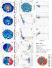 |
Fig. 1 NGC 1167: 2D maps (panels a)–f) and n)), radial intensity and EW of Hα (panels g) and h)), BPT diagrams (panels i) and j)), radial distribution of diagnostic line ratios (k) and l)), and the τ ratio (panel m)). In all 2D maps north is up and east to the left. The bar corresponds to 20′′. |
5. Discussion
5.1. 2D properties of gas and stars in the sample ETGs
The ℒ5 Gyr maps (Figs. 1n–C.31n) echo the well established fact that ETGs are dominated by an evolved stellar component throughout their optical extent. Even though there is a trend for an increasing luminosity contribution from stars younger than 5 Gyr towards the galaxy periphery, in agreement with the conclusions by, e.g., González Delgado et al. (2014a), panels n reveal, just like the inwardly increasing mass-weighted stellar age ⟨ t⋆ ⟩ ℳ (cf. Fig. B.3), that the bulk of the stellar component in ETGs has formed several Gyr ago.
Another insight from the Hα and EW(Hα) maps (panels b and c) is a diffuse wim component of low surface brightness over virtually the entire optical extent of our sample ETGs. Its cospatiality with the evolved underlying background is consistent with the notion that the diffuse ionizing field from the latter is an important driver of extranuclear wim emission. Following our pilot study in K12, this issue was addressed in more detail and on the basis of the robust statistics from this sample in P13, where we concluded that in about 40% of ETGs (type i), the properties of the extranuclear wim are indeed compatible with the pAGB photoionization hypothesis. The main argumentation in these studies was based on a combined analysis of the EW(Hα) and the τ ratio.
Figure A.1 shows for the first quantity that the photoionization by pAGB stars can reproduce the narrow range of EWs between EW (0.5 Å) and EW (~2.4 Å). This range can be further limited to ≃1 Å (≡⟨ EW⋆ ⟩) when taking into account the typical ⟨ t⋆ ⟩ ℳ (7–11 Gyr) of ETGs and making the reasonable assumption of a nearly solar metallicity (see discussion in Appendix A). Obviously, the condition
  ensures compliance of observations with predictions for pure pAGB models.
We note in passing that we do not invoke the presence or absence of LINER characteristics as an argument for or against pAGB photoionization, since it is known that they can be due to a variety of mechanisms, including shocks and starburst-driven outflows (see, e.g., Sharp & Bland-Hawthorn 2010, for a recent observational review). For example, the biconical wim component protruding several kpc outward from the nucleus of NGC 5966 in NE-SW direction (Fig. C.4; see K12 for a detailed discussion) shows LINER-typical emission-line ratios throughout and an EW(Hα) that is compatible with pure pAGB photoionization. Notwithstanding this fact, the morphology of this kinematically decoupled wim component is suggestive of large-scale shock excitation associated with gas outflow. The absence of ongoing SF throughout this ETG supports the idea that its gas outflow is powered by an AGN hosted in its LINER nucleus.
As for the τ ratio, a radial constancy around unity would ensure that pAGB stars are capable of supplying the ionizing photon budget that is necessary to sustain the observed Hα emission without need for any additional excitation source. The latter case would correspond to τ < 1, whereas a τ > 1 implies the escape of a fraction plf =1–τ-1 of the Lyman continuum radiation produced by the pAGB component (Sect. 1). As argued in Cid Fernandes et al. (2011), a relation between the EW(Hα) and τ-1 is to be expected, and this was found indeed from an analysis of Sloan Digital Sky Survey (SDSS) data (see their Fig. 5). Likewise, a tight anticorrelation between τ and EW(Hα) over nearly 3 dex, with the pAGB “equilibrium” line of τ ≃ 1 corresponding to EW(Hα) ≃ 1 Å (≡⟨ EW⋆ ⟩) was documented from the analysis of CALIFA IFS data in P13 (see their Fig. 2a).
It might superficially be argued that EW(Hα) and τ essentially reflect one and the same quantity and that they can therefore be used interchangeably in assessing the validity of the pAGB photoionization hypothesis. However, an appreciation of the a) geometry-dependent line-of-sight dilution effect of nuclear EWs in triaxial stellar systems and b) the large Lyc escape fraction in the majority of ETGs (see discussion in P13) challenge this simplistic view. For example, a consequence of the geometric dilution is that a radially constant EW(Hα) in the range between EW and EW can only be regarded as a proof for the validity of the pAGB photoionization hypothesis in the specific case of an oblate stellar system seen nearly face-on, or when in a triaxial stellar system the line-emitting wim is uniformly mixed with the EW-diluting stellar background. Whenever the wim occupies a smaller volume than the stars, the intrinsic EW(Hα) within a volume element is greater than the observed (projected) value. This cautionary note is essential for a proper evaluation of panels f where regions satisfying the condition  are depicted in light blue: pAGB photoionization can be regarded as the dominant gas excitation source in these regions only as long as the wim is cospatial with the stars and Lyc escape is negligible throughout. If any of these (far from self-evident) assumptions were invalid, then an additional excitation source (e.g., AGN or diffuse SF) would need to be postulated. In fact, comparison of panels b and c shows the strength of the line-of-sight EW dilution effect in several of our sample galaxies. NGC 5966 again offers an illustrative example: The biconical Hα emission in this system has its maximum at the peak of the stellar surface density (panel b), whereas the opposite is the case for the EW(Hα) (panel c). We note that a spatial anticorrelation between emission-line fluxes and EWs has also been documented and discussed in other triaxial systems, such as blue compact dwarf galaxies (see, e.g., Papaderos et al. 2002).
In P13 we showed that based on their EW(Hα) and τ profiles in their extranuclear zones (R⋆≥ 4′′; blue dots in panels g–m), ETGs span a broad, continuous sequence that can be tentatively grouped into two main classes based on radial EW(Hα) profiles (see schematic representation in Fig. 2). Type i ETGs (14 galaxies) are characterized by a nearly constant EW(Hα) of ≳1 Å out to their periphery, with the exception of a few systems where the EW shows a steep outer increase to EW(Hα) ≫ . Such systems, to which Gomes et al. (2015) assigned the notation i+, are the subject of a recent parallel CALIFA study (Gomes et al. 2016), which reveals that the EW excess is due to low-level star-forming activity in faint embedded spiral-like features. Type ii ETGs (18 galaxies), on the other hand, display very low (≤0.5 Å) EWs in their cores and typically positive EW gradients, approaching an EW(Hα) ≃ ⟨ EW⋆ ⟩ only in their outermost periphery (R⋆≳ 2 rp).
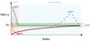 |
Fig. 2 Schematic representation of the two main classes of ETGs, as defined in P13. The EW(Hα) profiles of type i ETGs (blue), such as NGC 1167, show in their extranuclear component (beyond the radius range depicted by the vertical shaded area; typically ~2 kpc in our sample) nearly constant values within the narrow range between EW |

5.2. Nebular emission in type i ETGs
With regard to most type i ETGs in our sample, our results are consistent with (but, recalling our cautionary notes in the previous section, no proof of) the hypothesis that the diffuse ionizing photon field from the pAGB component is the main driver of extranuclear wim emission. Panels h in Fig. 1 and Figs. C.1–C.31 show that most isan determinations for type i ETGs satisfy the condition 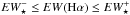 (shaded area in panels f), with most data points populating the EW strip around ⟨ EW⋆ ⟩. Consistent with this trend, most type i ETGs show a τ ≃ 1, with all data points located beneath τ = 2 (dashed horizontal line in panels m).
Two of the subclasses of type i+ ETGs are morphologically classified as S0 (NGC 1349 and NGC 3106), the third one as SA0 (NGC 1167). As shown in Gomes et al. (2016), the outer EW-enhanced zone of these systems (panel c) is due to photoionization by young stars over a fraction of between ~7% and ~47% of the galaxy area. We note that on the radial BPT ratio profiles (i.e., the isan-based [O iii ]/Hβ and [N ii]/Hα determinations in panels k and l) the outer star-forming zone of type i+ ETGs is clearly separable from the LINER-typical average for ETGs (gray strip) only when producing significant nebular emission (≥6 Å; NGC 1349 and NGC 3106; Figs. C.12 and C.13, respectively), but it is marginally traceable in NGC 1167 (Fig. 1), where the EW(Hα) (~3–4.5 Å) is just above EW. As discussed in Gomes et al. (2016), the spectroscopic BPT classification of type i+ ETGs is strongly dependent on the spectroscopic aperture used (or, equivalently, on the redshift of such a source). The presence of SF activity in the periphery of the three type i+ ETGs in our sample was noted in previous studies of the CALIFA collaboration (Sánchez 2014a), even though no explicit discussion was given to this subject because of the specific scope of these studies. For example, their analysis has established that the outer Hα rim in NGC 1349 is composed of several genuine Hii regions, that is, clumpy Hα entities containing a young ionizing stellar component with a luminosity fraction ≥20% and showing an EW(Hα) ≥ 6 Å (see, e.g., Sánchez et al. 2014b).
In addition to the three ETGs classified type i+, our sample contains a few other systems witnessing the potentially relevant role of SF over an extended radial zone or even galactic scale. The interpretation of pAGB photoionization dominating at all radii is challenged by singular or contiguous EW enhancements above ⟨ EW⋆ ⟩ in the extranuclear part of several ETGs. One such example is the S0 galaxy NGC 6081 (Fig. C.6c). This type i ETG shows LINER characteristics in its nucleus and intermediate zones (R⋆≲ 10′′) despite a contiguous weak (EW(Hα) ≲ 2.5 Å) SF rim all over its southwestern half. Still, isan determinations for the EW(Hα) and τ are consistent with a dominant contribution from pAGB photoionization, in agreement with Fig. C.6f, which indicates that sources other than pAGB stars dominate in less 7% of the area of the galaxy. Weak embedded SF patterns are also visible in three intermediate-morphology galaxies, NGC 7025 (Figs. C.11b and c), UGC 10205 (Figs. C.5b and c) and NGC 4003 (Figs. C.2b and c). In particular, Hα and EW(Hα) maps for NGC 7025 reveal a complex, low-level SF network with an  , surrounding an extended (R⋆~ 10′′) LINER/AGN core. LINER characteristics are also apparent in the intermediate zone of NGC 4003, whereas the nuclear region and the periphery of this ETG are dominated by SF. This case also illustrates how the area considered in the spectroscopic analysis can influence the spectroscopic classification, hence the relative role ascribed to different gas excitation mechanisms: sisp (i.e., higher-S/N) data capture only the intermediate LINER zone surrounding the SF nucleus, whereas the SF-dominated low surface brightness periphery of the galaxy becomes apparent on log ([O iii]/Hβ) and log ([N ii]/Hα) profiles only through isan determinations including lower-S/N spaxels.
According to our classification in Table 1, all nuclear properties of type i ETGs except for NGC 4003 and UGC 10205 fall into the LINER locus of BPT diagrams, just like our ETG sample as a whole. We note that sisp determinations on the log ([N ii]/Hα) vs. log ([O iii]/Hβ) and log (Σ[Sii]/Hα) vs. log ([O iii]/Hβ) diagrams (panels i and j) place the nuclei and intermediate zones close to the junction between the curves that demarcate the regions of maximum SF and AGN excitation.
Our study also shows that type i ETGs span a wide range in the EW(Hα) and spatial extent of their nuclear emission. A few of them show prominent nuclear wim components over ~6′′–10′′ (e.g., NGC 1167, NGC 5966, UGC 5771, and NGC 6146) with a peak EW of up to ~8 Å, whereas in others the nuclear nebular emission is rather compact (~FWHM) and faint (~⟨ EW⋆ ⟩). One example of extended nuclear emission over scales of ~4 kpc is seen in NGC 1167. In addition to the biconical wim protruding out to ~10 kpc from the nucleus of NGC 5966 in a direction perpendicular to the major axis, bipolar or unipolar wim lobes on kpc-scales from the nucleus are detected in UGC 10695 and NGC 6146. A robust spectroscopic and kinematical analysis of these extended, faint (EW(Hα) ≲ ⟨ EW⋆ ⟩) features is barely possible with the available CALIFA V500 data because of their low spectral and spatial resolution (FWHM ≥ 1 kpc at their distance of the four ETGs) and the moderate S/N. However, the absence of appreciable star formation in these ETG nuclei renders the interpretation of the detected wim lobes as AGN-driven outflows plausible, making them targets of considerable interest for follow-up studies exploring direct evidence for accretion-powered nuclear activity in LINER nuclei. Spatially resolved IFS studies of high-excitation (i.e., AGN-specific) emission lines in the nuclear and circumnuclear region of these candidate AGN (following the approach by Müller-Sánchez et al. 2011), supplemented by kinematical modeling of biconical gas outflows that might be emanating from their narrow-line regions (e.g., Fischer et al. 2013), could provide key insights in this respect.
5.3. Deficit of nebular emission in type ii ETGs
The nature of type ii ETGs – systems commonly referred to as ETGs without nebular emission – is enigmatic. These galaxies make up about 60% (18 of 32) of our sample and are classified on the condition ⟨ τ ⟩ ≥ 2 in their extranuclear component (cf. P13). Nebular emission in these systems is only detectable after accurate fitting and subtraction of the local underlying stellar SED, which clearly is a demanding task, given its extreme faintness. This is particularly true for the virtually wim-evacuated cores of these ETGs, where the EW(Hα) has its minimum, after which it gradually rises to levels ≳ up to ⟨ EW⋆ ⟩ in the outermost galaxy periphery (~2rp). These positive EW(Hα) gradients, as distinctive features of type ii ETGs, were interpreted by P13 as manifestation of the radius-dependent structure and physical conditions of the gas in these systems (volume-filling factor, porosity, and 3D distribution; electron density and ionization parameter). Panels f show that the low EW(Hα) within typically more than 80% of the spectroscopically studied area of type ii ETGs is incompatible with pAGB photoionization, if case B recombination for standard gas conditions (ne = 100 cm-3, Te = 104 K) is assumed, which supports our previous conclusion in P13 that most of the ionizing photons generated by the pAGB component escape without being reprocessed into nebular emission. As a comparison, on average 65% of the area of a type i ETG is consistent with the hypothesis that their gas is being photoionized by pAGB stars.
Diagnostic emission-line ratios and their radial distribution in type ii ETGs have to be considered in the light of their large uncertainties, even after averaging of sisp determinations within morphology-adapted irregular annuli (isan). Despite the scatter of typically 0.3 dex for isan data, panels i and j consistently show that type ii ETGs are in practice indistinguishable from type i ETGs by their nearly radially constant LINER-typical BPT ratios.
Type ii ETGs also feature a considerable heterogeneity in their nuclear properties: Panels b and c show that in some of these systems a compact but extended (≳3·PSF) nuclear Hα excess is reliably detected, for example, in NGC 2918, NGC 6150, NGC 6173, NGC 6515, NGC 7550 and, more impressively, in UGC 11958 and NGC 6338. In the majority of type ii ETGs, however, nebular traces of nuclear activity are almost absent, with an EW(Hα) marginally above that of the diffuse wim and at the edge of the detectability (0.1–0.3 Å).
Whereas individual sisp data points are generally subject to prohibitively large relative uncertainties (above 100% at EWs < 0.3 Å) in the peripheral zones, the averaging of hundreds of such determinations within isan shows a faint substrate of wim with an  . This is augmented by determinations of emission-line fluxes based on azimuthally binned isan segments (Fig. B.5) or the collapsed spectrum within each isan, after correcting for local stellar motions (Fig. B.6). It should be noted, on the other hand, that the angular resolution of our data and the faintness of the wim does not allow us to determine whether part of the nebular emission originates from higher-density Hii-region clumps within a more tenuous wim component.
5.3.1. Accretion-powered nuclear activity in ETG/LINERs
Whether or not LINER nuclei in ETGs harbor an AGN is subject of an intense longstanding controversy, with antipodal conclusions reached, including the radical rejection of the hypothesis of accretion-powered nuclear activity in favor of pure pAGB photoionization (cf. Introduction). However, a first reservation toward the latter statement comes from the established relation between the velocity dispersion of galaxy spheroids and the mass of their supermassive black hole (SMBH; see Merritt & Ferrarese 2001, for a review), which is estimated to range between a few 107M⊙ and up to ~1010M⊙. If this were true, a minimum amount of gas would in principle suffice to sustain accretion-powered nuclear activity, perhaps in the form of a weak, radiatively inefficient LLAGN. As this study shows, diffuse wim is present, even in type ii ETGs, which leaves space for the AGN hypothesis. Indirect observational support for the latter comes from the biconical/unipolar wim lobes in three type i ETGs of our sample (Sect. 5.2), which are consistent with AGN-driven gas outflows. Additionally, in one type i ETG (NGC 1167) the presence of an AGN is indicated by a radio jet (e.g., Sanghera et al. 1995; Giovannini et al. 2001). Among type ii ETGs, radio-continuum data for NGC 6150 and UGC 11958 (cf. Table 1) also record the energy release by an AGN. For example, the line-weak (EW(Hα) ~ 3.5 Å) LINER nucleus of UGC 11958 powers a ≳100 kpc double-lobe radio continuum halo detected at 1.4 GHz with the VLA (Comins & Owen 1991) with a large (~40 kpc) central cavity of hot (~1 keV), pressure-driven X-ray emitting plasma (Worrall et al. 2007), which clearly indicates energetic action by an AGN.
How to reconcile the weakness of optical emission lines in ETG/LINERs with signatures of strong accretion-powered nuclear activity in radio- and X-ray wavelengths poses an enigma. As first pointed out in P13, the seemingly trivial fact that more than one half of the ETGs lack nebular emission as a result of an insufficient mean gas density and/or high gas porosity has far-reaching consequences for our understanding of accretion-powered nuclear activity in these systems: In the presence of extensive Lyc photon escape, implied by the lack of gas, emission-line luminosities and EWs, upon which estimates of accretion rates and SMBH masses rely, are reduced by more than an order of magnitude. An additional effect acting toward diminishing nuclear EWs (or any photometric signs of nuclear activity) in these triaxial stellar systems is dilution by the stellar background along the line of sight (P13). According to our study in P13, the line weakness of ETG/LINER nuclei is therefore no clear evidence for the weakness or absence of AGN in these systems. In the light of this conclusion and from the evidence presented in Sects. 5.2 and 5.3, it is therefore conceivable that different gas excitation mechanisms (photoionization by AGN, OB stars and pAGB sources; shocks) – each of them with a different relative contribution in different radial zones – are simultaneously at work. An exploration of this question with deep, higher spectral resolution IFS data clearly is of great interest.
5.4. Stellar and gas kinematics in ETGs
A detailed study of stellar and gas kinematics in the CALIFA galaxy survey is subject of several ongoing investigations within the CALIFA collaboration (García-Lorenzo et al. 2015; Sánchez-Blázquez et al. 2014, Falcón-Barroso et al., in prep.), which uses higher-resolution (V1200; FWHM ~ 2.3 Å) IFS data and to which we refer for detailed information. The brief remarks below are merely meant to further highlight the kinematical diversity of our sample ETGs.
As already revealed by several studies before, most notably in the the SAURON and Atlas3D projects (cf., e.g., Sarzi et al. 2006, 2010), ETGs display a variety in their stellar kinematics patterns from regular rotation along the semi-major axis to nearly pressure-supported galaxies with subtle, if any, signs of ordered motions.
Panels d and e of Figs. 1–C.31 show that in most (27) of the ETGs studied here stellar kinematics are dominated by rotation. The velocity difference Δv⋆ = (va + vr)/2 between the receding (vr) and approaching (va) part of these systems is typically on the order of 200 km s-1. Interestingly, weak rotation at 60 km s-1≲Δv⋆≲ 110 km s-1 along the minor galaxy axis is clearly detected in three type ii ETGs (NGC 6173, NGC 6338, and NGC 7236). Five galaxies (UGC 10695, NGC 6515, UGC 11958, NGC 7550, and UGC 29) appear to be dominated by random motions. We note, however, that the low spectral resolution and moderate S/N of our CALIFA V500 IFS data do not permit us to firmly rule out some degree of rotation in these systems. Higher spectral resolution CALIFA data (Falcón-Barroso et al., in prep.), enabling a detailed study of stellar line-of-sight velocity patterns and possible kinematical distortions (e.g., counter-rotating cores) over the full set of CALIFA ETGs, are necessary for a conclusive assessment of this matter. An interesting question in this respect is how type i/i+ and type ii ETGs compare to each other with respect to their angular momentum per unit mass in the definition by Emsellem et al. (2007). These authors have shown that fast rotators in the SAURON sample tend to be lower luminosity ETGs with well-aligned photometric and kinematic axes, whereas slow rotators typically exhibit significant misalignments and kinematically decoupled cores.
A comparative study of type i/i+ and ii ETGs with regard to the kinematics of their wim is obviously another key task that could help understanding whether gas is internally produced, in the course of stellar evolution, or accreted from captured satellites. The spiral-arm-like SF features in type i+ ETGs, or faint embedded SF patterns in several other ETGs are suggestive, but no proof, of the gas accretion scenario. With regard to the discussion below, it is important to bear in mind that the non-detection of ordered gas motions in most of our sample ETGs (especially those classified type ii) may reflect observational limitations that are due to the extreme faintness of the wim (see also Sect. 5.5, in particular our remarks on the type i+ ETG NGC 160 in Fig. 3). Clearly, a detailed study of ionized-gas kinematics is, in particular in type ii ETGs, a formidable task that can only be pursued with a high S/N (typically ≥60 at 6390–6490 Å) and/or spatially binned data (e.g., García-Lorenzo et al. 2015).
Some noteworthy trends are apparent from the analysis of our low-resolution V500 data, however: In roughly one third (11) of the sample ETGs (eight classified type i and in the three type i+) gas kinematics are consistent with rotation aligned with stellar motions, albeit slightly perturbed kinematical patterns. For instance, in NGC 1167 the wim rotation axis appears slightly tilted relative to the stellar one, with a possible spatial offset between the photometric and kinematical center. In three type i ETGs (NGC 5966, UGC 10695, and UGC 10905) gas kinematics appear to be dominated by outflows, and a suggestion for an outflowing gas component is also present in NGC 6146. Of the three type ii ETGs showing stellar rotation perpendicular to the major axis, we did not detect gas motions in NGC 6173 and NGC 7236, while in NGC 6338 there is a trace of a compact rotating (~70 km s-1) wim component, centered on the optical nucleus. Likewise, in NGC 7550 gas rotation at Δvg~ 80 km s-1 can be traced within the central ~7 kpc of a pressure-supported stellar host. Summarizing, this study further highlights and adds observational insight into the kinematical diversity of the ETG galaxy family (see also, e.g., Sarzi et al. 2006; Katkov et al. 2014). On the other hand, the evidence from Figs. 1 and C.1–C.31 permits identifying broad kinematical trends in the three ETG types: Type i and i+ ETGs are generally rotation supported with many cases of perturbed rotational patterns or outflows in their wim, whereas type ii ETGs exhibit either rotationally or pressure-supported stellar kinematics and generally lack distinguishable kinematic patterns in their ionized gas. Table 1 (Col. 14) includes a descriptive three-character kinematical classification, with r denoting rotation-dominated kinematics, p perturbed rotational patterns, o gas outflows, and n no distinguishable patterns or pressure-supported stellar kinematics. The first and third character refer to the kinematics of stars and gas, respectively, and the second character indicates in the case of stellar rotation (r or p) whether the kinematic and photometric major axes are roughly aligned (∥) or not (∦).
5.5. Equivalent width bias on ETG taxonomy
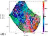 |
Fig. 3 Emission-line-free stellar continuum a), Hα flux in 10-16 erg s-1 cm-2b) and Hα+[Nii] line-of-sight velocity in km/s c) of the type i+ ETG NGC 160, as inferred from processing of CALIFA (v1.5) V500 with Porto3D. The overlaid contours delineate the EW(Hα) morphology of the galaxy and reach from 4 Å to 21 Å in steps of 3 Å. North is up and east to the left. |
A central result from our study in P13 is the considerable radial dependence of the EW(Hα) in many ETGs (panels c and h): A distinctive property of several type ii ETGs is their almost wim-emission free cores and their outwardly increasing EW(Hα), reaching in some cases readily detectable levels (~⟨ EW⋆ ⟩) in their periphery alone. Although type i ETGs show on average an EW(Hα) ≃ ⟨ EW⋆ ⟩ in their extranuclear component, there are several cases in our sample where the EW(Hα) significantly varies within different radial zones. This is particularly true for the two-zone wim morphology of type i+ ETGs: An illustrative example is NGC 1349, showing a constant EW(Hα) ≃ ⟨ EW⋆ ⟩ for R⋆≤ 8′′ (3.4 kpc), in agreement with pure pAGB photoionization, whereas in the periphery (R⋆~ 16–20′′) the EW(Hα) rises to ≳6 Å, revealing an extra ionizing field produced by ongoing SF activity (Sect. 5.2).
In fact, the intuitive expectation that emission-line EWs in ETGs are spatially correlated with the surface brightness of the stellar background, invariably attaining their peak value at the ETG nuclei, is disproved by panels c and h of Figs. 1–C.31. A comparison of panels a and b with panel c in many cases reveals an inverse trend with the EW(Hα) showing – in contrast to the stellar and Hα surface brightness – a low or even minimum value in the nuclear region (e.g., Fig. C.4). This spatial anticorrelation between the intensity and EW of emission lines has been documented and discussed in studies of low-mass starburst galaxies (Papaderos et al. 1998, 2002) and, in the case of ETGs, it can be partly attributed to line-of-sight dilution of nuclear EWs by a triaxial stellar host (P13). As we pointed out in P13, this geometric effect introduces a selection bias against the detection of nuclear activity in galaxy spheroids, since emission-line EWs (and obviously any other manifestation of energy release by an AGN in UV-NIR wavelengths) in their centers are diluted not only by the local stellar background, but also by the integrated line-of-sight luminosity of stars. Since this geometric dilution effect amplifies an observational bias stemming from the high Lyc photon escape fraction in type ii ETG nuclei, caution is needed when arguing that the weakness of nuclear emission-lines and EWs in ETGs/LINERs is evidence for weak or non-existent accretion-powered nuclear activity.
In the light of these two effects, analogous considerations also apply to the usage of the EW(Hα) as discriminator between AGN and retired galaxies in the context of the WHAN classification (Cid Fernandes et al. 2011): A nuclear EW(Hα) between EW and EW, that is, an EW in the range of predicted values for pAGB photoionization in retired galaxies, does not necessarily rule out an AGN as the dominant excitation source of the wim. The true nuclear EW (i.e., the EW after correcting for the geometric dilution and Lyc escape bias) could exceed the observed (projected) EW by more than one order of magnitude, shifting on the WHAN diagram a seemingly weak (low-luminosity) AGN into the strong AGN regime (cf. our discussion in P13).
It is also worth contemplating the observational biases that the EW detection limit may have on taxonomical studies of ETGs. We note that extranuclear nebular emission would not have been detected in any type ii ETG if our analysis were restricted to an EW(Hα) ≥ 1 Å. Because of the geometrical EW dilution effect, even the compact Hα-emitting nuclei of many type i and type ii ETGs (e.g., in NGC 1349, UGC 8234, NGC 6515, and NGC 7025) vanish to EWs ≤ 1 Å, and would have gone undetected if such a quality-ensuring EW(Hα) threshold would have been adopted. By that cutoff, all but three type ii ETGs (NGC 6338, UGC 11958, and NGC 7550) would have been classified as gas-free passive galaxies (see definition by Cid Fernandes et al. 2011). Even though the thin higher EW outer rim of nebular emission would have been recovered in type i+ ETGs, this alone would not have shown the extended nature of the circumnuclear wim component.
The importance of this EW-threshold bias may be illustrated by inspecting the wim morphology and kinematics maps of NGC 160, a type i+ ETG that will be subject of a forthcoming article of this series. The overlaid contours in the three panels of Fig. 3 depict the EW(Hα) morphology of the galaxy and reach from 4 Å to 21 Å in steps of 3 Å. While a substrate of diffuse (0.5 ≲ EW(Hα) [Å] ≲ 2) wim is present almost everywhere in the central part of the galaxy, the bulk of Hα emission is confined to an extended (~60″ × 40″) rim surrounding the low surface brightness stellar periphery (see also García-Lorenzo et al. 2015). An EW detection threshold of 4 Å (i.e. ≥; outermost contour in all panels) would obviously only allow for the recovery of the outer rim, leading to the erroneous conclusion that this ETG is completely devoid of wim almost throughout its optical extent, out to ~24 mag/Λ″ in the SDSS r band (cf. Breda et al., in prep.). A further implication would have been the complete rejection of the pAGB photoionization hypothesis, since this can only be tested for an EW detection threshold ≤, and the conclusion that photoinization by OB stars is the sole gas excitation mechanism in this ETG. An EW threshold ≳ would also result in a severely incomplete view of the overall gas kinematics everywhere but in the EW-enhanced rim, with obvious implications for the dynamical modeling of such a galaxy.
6. Summary and conclusions
We have investigated in significantly more detail the sample of 32 CALIFA ETGs that we discussed in P13, which was focused on their radial EW(Hα) distribution and Lyc photon escape fraction. We studied here the 2D properties of their diffuse warm interstellar medium (wim) to gain insight into its excitation mechanism(s) and provide additional observational constraints aiming at systematizing the physical properties of these systems. Among other quantities derived by applying our IFS data processing pipeline Porto3D to low spectral resolution (~6 Å FWHM) CALIFA data, we presented for each galaxy Hα intensity and EW maps and radial profiles. We also analyzed the nuclear and extranuclear nebular emission of the wim using diagnostic line ratios. A comparison sample of CALIFA galaxies of intermediate-to-late type is meant to illustrate how various observables of interest change from bulge-dominated ETGs to disk-dominated star-forming (SF) galaxies. Additionally, we briefly discussed the kinematical properties of gas and stars in our sample.
The main conclusions from this study may be summarized as follows:
i): The analyzed ETGs contain an extendedwim component displaying a considerablediversity in its mean EW(Hα) and its radialgradients. As we discussed in P13, our ETG sample can betentatively subdivided into two groups. The extranuclearwim of the first class (type i) ischaracterized by a nearly constant EW(Hα) of~1 Å, with the exception of afew systems (i+, in the notation by Gomeset al. 2016) showinga steep EW(Hα) increase in their pe-riphery. The second group (type ii)displays almost wim-evacuated cores and a grad-ual increase of the EW(Hα) outward to≲1 Å.
ii): The ETGs studied here also display a rich diversity in their kinematics. The majority (27 out of 32) of our sample ETGs exhibit stellar kinematics dominated by rotation, with three systems showing a kinematic major axis aligned with the photometric minor axis. Type i and i+ ETGs are generally rotation supported. with many cases of perturbed rotational patterns or outflows in their ionized gas, whereas the class of type ii ETGs contains both rotationally and pressure supported stellar systems, which generally lack distinguishable kinematic patterns in their ionized gas.
iii): We computed the time evolution of the EW(Hα) for various star formation histories (SFHs) and stellar metallicities based on an evolutionary synthesis model and assuming case B recombination and standard conditions for the gas. We found that SFHs involving an exponentially decreasing star formation rate since 13 Gyr can reproduce the low (~1 Å) EW(Hα)’s in the extranuclear component of present-day ETGs when a short (≤1 Gyr) e-folding timescale is adopted. In this case, the Lyman continuum (Lyc) output predicted to arise from the pAGB stellar component is sufficient to power the excitation of the diffuse wim. SFHs involving a longer e-folding timescale (e.g., ≥3 Gyr) imply higher EW(Hα)’s than observed.
iv): For most type i ETGs, photoionization by the evolved pAGB stellar background offers a consistent but not necessarily compelling explanation for the observed EW(Hα)s and τ ratios (the inverse ratio of the observed Hα luminosity to that predicted for pure pAGB photoionization). We point out that Lyc photon escape and geometric line-of-sight dilution of EWs (cf. P13) could conspire in such a way as to reproduce the low (≃1 Å) and nearly constant EW(Hα) in the extranuclear component of type i ETGs, thereby mimicking a predominance of pAGB photoionization to the excitation of their diffuse ionized gas component, while hiding a potentially important role by AGN and low-level SF. The presence of the latter in the extranuclear component of several ETGs from our sample is clearly indicated from EW(Hα) maps.
v): The radial EW(Hα) gradients and the extreme faintness of nebular emission in ETGs, in particular in systems classified type ii, leads to biases that affect the detectability of the extended wim component and the interpretation of its excitation mechanisms. We point out that nebular emission in the centers of type ii ETGs will generally evade detection below an EW threshold of ~0.5–1.0 Å, which could lead to the conclusion that these systems are entirely devoid of wim and to their erroneous classification as passive galaxies.
vi): The radial distribution of diagnostic line ratios indicates that in their majority, ETGs show LINER-specific spectroscopic properties both in their nuclear and extranuclear zones. Our sample includes a few notable exceptions (in particular, type i+ ETGs), however, where a significant contribution by star formation in peripheral zones is reflected both in radial log ([N ii]/Hα), log ([O iii]/Hβ) and τ profiles, and EW(Hα) maps. This calls attention to the heterogeneity of the ETG class, pointing to a complex interplay between the 3D properties of the wim and the combined action of various gas ionization sources, such as shocks, OB stars, and the evolved pAGB component. As we argued in Papaderos et al. (2013) and further detailed here, the weakness of nebular emission lines in ETG nuclei is not compelling evidence for the absence of accretion-powered nuclear activity in these systems. In fact, radio-continuum and/or X-ray data, or bipolar or unipolar wim lobes protruding several kpc from the LINER nuclei of 25% of our sample ETGs, witness the energetic action of an AGN. Summarizing, the results and consideration presented in this study are incompatible with the hypothesis that the global gas excitation patterns in ETGs are controlled by one single dominant mechanism.
Since it is now recognized that LINER-specific emission-line ratios are not confined to galaxy nuclei (e.g., Sharp & Bland-Hawthorn 2010; Kehrig et al. 2012; Papaderos et al. 2013; Singh et al. 2013), a more adequate acronym would be “low-ionization emission-line regions” (LIERs).
For the sake of brevity we refer in the following to all ionizing point sources arising at and beyond the post-AGB phase as pAGB stars.
Munich Image Data Analysis System, provided by the European Southern Observatory (ESO).
STARLIGHT & SEAGal: http://www.starlight.ufsc.br/
Acknowledgments
This paper is based on data from the Calar Alto Legacy Integral Field Area Survey, CALIFA (http://califa.caha.es), funded by the Spanish Ministery of Science under grant ICTS-2009-10, and the Centro Astronómico Hispano-Alemán. JMG acknowledges support by Fundação para a Ciência e a Tecnologia (FCT) through the Fellowship SFRH/BPD/66958/2009 and POPH/FSE (EC) by FEDER funding through the program Programa Operacional de Factores de Competitividade (COMPETE). PP is supported by FCT through the Investigador FCT Contract No. IF/01220/2013 and POPH/FSE (EC) by FEDER funding through the program COMPETE. JMG, PP, IB and SNdR also acknowledge support by FCT under project FCOMP-01-0124-FEDER-029170 (Reference FCT PTDC/FIS-AST/3214/2012), funded by FCT-MEC (PIDDAC) and FEDER (COMPETE). They also acknowledge support by the exchange programme “Study of Emission-Line Galaxies with Integral-Field Spectroscopy” (SELGIFS, FP7-PEOPLE-2013-IRSES-612701), funded by the EU through the IRSES scheme. S.F.S. acknowledges support from CONACyT-180125 and PAPIIT-IA100815 grants. Support for L.G. is provided by the Ministry of Economy, Development, and Tourism’s Millennium Science Initiative through grant IC120009, awarded to The Millennium Institute of Astrophysics, MAS. L.G. acknowledges support by CONICYT through FONDECYT grant 3140566. C.J.W. acknowledges support through the Marie Curie Career Integration Grant 303912. R.G.B. is supported by the Spanish Ministerio de Ciencia e Innovación under grant AYA2010-15081. R.A. Marino is funded by the Spanish program of International Campus of Excellence Moncloa (CEI). I.M. acknowledges financial support by the Junta de Andalucía through project TIC114, and the Spanish Ministry of Economy and Competitiveness (MINECO) through projects AYA2010-15169 and AYA2013-42227-P. A.d.O. acknowledges financial support from the Spanish grants AYA2010-15169 and AYA2013-42227-P. J.F.-B. acknowledges support from grant AYA2013-48226-C3-1-P from the Spanish Ministry of Economy and Competitiveness (MINECO). The starlight project is supported by the Brazilian agencies CNPq, CAPES, and FAPESP. We benefited from stimulating discussions with several members of the CALIFA collaboration. This research made use of the NASA/IPAC Extragalactic Database (NED) which is operated by the Jet Propulsion Laboratory, California Institute of Technology, under contract with the National Aeronautics and Space Administration.
References
- Allen, M. G., Groves, B. A., Dopita, M. A., Sutherland, R. S., & Kewley, L. J. 2008, ApJS, 178, 20 [Google Scholar]
- Alongi, M., Bertelli, G., Bressan, A., et al. 1993, A&AS, 97, 851 [NASA ADS] [Google Scholar]
- Annibali, F., Bressan, A., Rampazzo, R., et al. 2010, A&A, 519, A40 [NASA ADS] [CrossRef] [EDP Sciences] [Google Scholar]
- Arnold, J. A., Romanowsky, A. J., Brodie, J. P., et al. 2014, ApJ, 791, 80 [NASA ADS] [CrossRef] [Google Scholar]
- Bacon, R., Copin, Y., Monnet, G., et al. 2001, MNRAS, 326, 23 [NASA ADS] [CrossRef] [Google Scholar]
- Baldwin, J. A., Phillips, M. M., & Terlevich, R. 1981, PASP, 93, 5 [NASA ADS] [CrossRef] [EDP Sciences] [Google Scholar]
- Barrera-Ballesteros, J. K., Falcón-Barroso, J., García-Lorenzo, B., et al. 2014, A&A, 568, A70 [NASA ADS] [CrossRef] [EDP Sciences] [Google Scholar]
- Bender, R., Surma, P., Döbereiner, S., Möllenhoff, C., & Madejsky, R. 1989, A&A, 217, 35 [NASA ADS] [Google Scholar]
- Binette, L., Magris, C. G., Stasińska, G., & Bruzual, A. G. 1994, A&A, 292, 13 [NASA ADS] [Google Scholar]
- Bregman, J. N. 1978, ApJ, 224, 768 [NASA ADS] [CrossRef] [Google Scholar]
- Bressan, A., Fagotto, F., Bertelli, G., & Chiosi, C. 1993, A&AS, 100, 647 [NASA ADS] [Google Scholar]
- Bruzual, G., & Charlot, S. 2003, MNRAS, 344, 1000 [NASA ADS] [CrossRef] [Google Scholar]
- Cappellari, M., Emsellem, E., Krajnovic, D., et al. 2011, MNRAS, 413, 813 [NASA ADS] [CrossRef] [Google Scholar]
- Castellanos, M., Díaz, A. I., & Terlevich, E. 2002, MNRAS, 329, 315 [NASA ADS] [CrossRef] [Google Scholar]
- Chabrier, G. 2003, PASP, 115, 763 [NASA ADS] [CrossRef] [Google Scholar]
- Cid Fernandes, R., Mateus, A., Sodré, L., Stasińska, G., & Gomes, J. M. 2005, MNRAS, 358, 363 [NASA ADS] [CrossRef] [Google Scholar]
- Cid Fernandes, R., Asari, N. V., Sodré, L., et al. 2007, MNRAS, 375, L16 [NASA ADS] [CrossRef] [Google Scholar]
- Cid Fernandes, R., Stasinka, G., Schlickmann, M. S., et al. 2010, MNRAS, 403, 1036 [NASA ADS] [CrossRef] [Google Scholar]
- Cid Fernandes, R., Stasińska, G., Mateus, A., et al. 2011, MNRAS, 413, 1687 [NASA ADS] [CrossRef] [Google Scholar]
- Cid Fernandes, R., González Delgado, R. M., García-Benito, R., et al. 2014, A&A, 561, A130 [NASA ADS] [CrossRef] [EDP Sciences] [Google Scholar]
- Clemens, M. S., Bressan, A., Panuzzo, P., et al. 2009b, MNRAS, 392, 982 [NASA ADS] [CrossRef] [Google Scholar]
- Comins, N. F., & Owen, F. N. 1991, ApJ, 382, 108 [NASA ADS] [CrossRef] [Google Scholar]
- Demoulin-Ulrich, M., Butcher, H. R., & Boksenberg, A. 1984, ApJ, 285, 527 [NASA ADS] [CrossRef] [Google Scholar]
- di Seregho Alighieri, S., Trinchieri, G., & Brocato, E. 1990, in Windows on Galaxies, eds. G. Fabbiano, J. S. Gallagher, & A. Renzini (Dordrecht: Kluwer), Astrophys. Space Sci. Libr., 160, 301 [Google Scholar]
- Dopita, M. A., & Sutherland, R. S. 1995, ApJ, 455, 468 [NASA ADS] [CrossRef] [Google Scholar]
- Emsellem, E., Cappellari, M., Krajnović, D., et al. 2007, MNRAS, 379, 410 [Google Scholar]
- Eracleous, M., Hwang, J. A., & Flohic, H. M. L. G. 2010, ApJ, 711, 796 [NASA ADS] [CrossRef] [Google Scholar]
- Fagotto, F., Bressan, A., Bertelli, G., & Chiosi, C. 1994a, A&AS, 104, 365 [NASA ADS] [Google Scholar]
- Fagotto, F., Bressan, A., Bertelli, G., & Chiosi, C. 1994b, A&AS, 105, 29 [NASA ADS] [Google Scholar]
- Fagotto, F., Bressan, A., Bertelli, G., & Chiosi, C. 1994c, A&AS, 105, 39 [NASA ADS] [Google Scholar]
- Falcón-Barroso, J., Sánchez-Blázquez, P., Vazdekis, A., et al. 2011, A&A, 532, A95 [NASA ADS] [CrossRef] [EDP Sciences] [Google Scholar]
- Finkelman, I., Brosch, N., Funes, J. G., Kniazev, A. Y., & Väisänen, P. 2010, MNRAS, 407, 2475 [NASA ADS] [CrossRef] [Google Scholar]
- Fischer, T. C., Crenshaw, D. M., Kraemer, S. B., & Schmitt, H. R. 2013, ApJS, 209, 1 [NASA ADS] [CrossRef] [Google Scholar]
- García-Benito, R., Zibetti, S., Sánchez, S. F., et al. 2015, A&A, 576, A135 [NASA ADS] [CrossRef] [EDP Sciences] [Google Scholar]
- García-Lorenzo, B., Márquez, I., Barrera-Ballesteros, J. K., et al. 2015, A&A, 573, A59 [NASA ADS] [CrossRef] [EDP Sciences] [Google Scholar]
- Giovannini, G., Cotton, W. D., Feretti, L., et al. 2001, ApJ, 552, 508 [NASA ADS] [CrossRef] [Google Scholar]
- Girardi, L., Bressan, A., Chiosi, C., Bertelli, G., & Nasi, E. 1996, A&AS, 117, 113 [NASA ADS] [CrossRef] [EDP Sciences] [Google Scholar]
- Gomes, J. M., Papaderos, P., Kehrig, C., et al. 2015, in Galaxies in 3D across the Universe, IAU Symp., 309, 105 [Google Scholar]
- Gomes, J. M., Papaderos, P., Vílchez, J. M., et al. 2016, A&A, 585, A92 [NASA ADS] [CrossRef] [EDP Sciences] [Google Scholar]
- González-Delgado, R. M., Pérez, E., Diaz, A., et al. 1995, ApJ, 439, 604 [NASA ADS] [CrossRef] [Google Scholar]
- González Delgado, R. M., Pérez, E., Cid Fernandes, R., et al. 2014a, A&A, 562, A47 [NASA ADS] [CrossRef] [EDP Sciences] [Google Scholar]
- González Delgado, Cid Fernandes, García-Benito, et al. 2014b, ApJ, 791, L16 [NASA ADS] [CrossRef] [Google Scholar]
- Heckmann, T. M. 1980, A&A, 87, 152 [NASA ADS] [Google Scholar]
- Ho, L. C. 1999, Adv. Space Res., 23, 813 [NASA ADS] [CrossRef] [Google Scholar]
- Ho, L. C. 2008, ARA&A, 46, 475 [NASA ADS] [CrossRef] [Google Scholar]
- Ho, L. C., Filippenko, A. V., & Sargent, W. L. 1995, ApJS, 98, 477 [NASA ADS] [CrossRef] [Google Scholar]
- Husemann, B., Jahnke, K., Sánchez, S. F., et al. 2013, A&A, 549, A87 [NASA ADS] [CrossRef] [EDP Sciences] [Google Scholar]
- Iglesias-Páramo, J., Vílchez, J. M., Galbany, L., et al. 2013, A&A, 553, L7 [NASA ADS] [CrossRef] [EDP Sciences] [Google Scholar]
- Katkov, I. Y., Silćhenko, O. K., & Afanasiev, V. L. 2014, MNRAS, 438, 2798 [NASA ADS] [CrossRef] [Google Scholar]
- Kauffmann, G., Heckman, T. M., Tremonti, C., et al. 2003, MNRAS, 346, 1055 [Google Scholar]
- Kaviraj, S., Schawinski, K., Devriendt, J. E. G., et al. 2007, ApJS, 173, 619 [NASA ADS] [CrossRef] [Google Scholar]
- Kaviraj, S., Khochfar, S., Schawinski, K., et al. 2008, MNRAS, 388, 67 [NASA ADS] [CrossRef] [Google Scholar]
- Kehrig, C., Monreal-Ibero, A., Papaderos, P., et al. 2012, A&A, 540, A11 (K12) [NASA ADS] [CrossRef] [EDP Sciences] [Google Scholar]
- Kelz, A., Verheijen, M. A. W., Roth, M. M., et al. 2006, PASP, 118, 129 [NASA ADS] [CrossRef] [Google Scholar]
- Kewley, L. J., Dopita, M. A., Sutherland, R. S., Heisler, C. A., & Trevena, J. 2001, ApJ, 556, 121 [Google Scholar]
- Kim, D. 1989, ApJ, 346, 653 [NASA ADS] [CrossRef] [Google Scholar]
- Kormendy, J., Fisher, D. B., Cornell, M. E., & Bender, R. 2009, ApJ, 182, 216 [NASA ADS] [Google Scholar]
- Kotulla, R., Fritze, U., Weilbacher, P., & Anders, P. 2009, MNRAS, 396, 462 [NASA ADS] [CrossRef] [Google Scholar]
- Krajnovic, D., Karick, A. M., Davies, R. L., et al. 2013, MNRAS, 2012, 433, 2812K [Google Scholar]
- Kulkarni, S. R., Ofek, E. O., Neill, J. D., Zheng, Z., & Juric, M. 2014, ApJ, 797, 70 [NASA ADS] [CrossRef] [Google Scholar]
- Le Borgne, J.-F., Bruzual, G., Pelló, R., et al. 2003, A&A, 402, L433 [CrossRef] [EDP Sciences] [Google Scholar]
- Leitherer, C., Schaerer, D., Goldader, J. D., et al. 1999, ApJ, 123, 3 [NASA ADS] [Google Scholar]
- Macchetto, F., Pastoriza, M., Caon, N., et al. 1996, A&AS, 120, 463 [NASA ADS] [CrossRef] [EDP Sciences] [Google Scholar]
- Marino, R. A., Rosales-Ortega, F. F., Sánchez, S. F., et al. 2013, A&A, 559, A114 [NASA ADS] [CrossRef] [EDP Sciences] [Google Scholar]
- Mast, D., Rosales-Ortega, F. F., Sánchez, S. F., et al. 2014, A&A, 561, A129 [NASA ADS] [CrossRef] [EDP Sciences] [Google Scholar]
- Mathews, W. G., & Baker, J. C. 1971, ApJ, 170, 241 [NASA ADS] [CrossRef] [Google Scholar]
- Merritt, D., & Ferrarese, L. 2001, ApJ, 547, 140 [NASA ADS] [CrossRef] [Google Scholar]
- Müller-Sánchez, F., Prieto, M. A., Hicks, E. K. S., et al. 2011, ApJ, 739, 69 [NASA ADS] [CrossRef] [Google Scholar]
- Noeske, K. G., Papaderos, P., Cairos, L. M., & Fricke, K. J. 2003, A&A, 410, 48 [Google Scholar]
- Noeske, K. G., Koo, D. C., Phillips, A. C., et al. 2006, ApJ, 640, 143 [Google Scholar]
- Papaderos, P., Izotov, Y. I., Fricke, K. J., Thuan, T. X., & Guseva, N. G. 1998, A&A, 338, 43 [NASA ADS] [Google Scholar]
- Papaderos, P., Izotov, Y. I., Thuan, T. X., et al. 2002, A&A, 393, 461 [NASA ADS] [CrossRef] [EDP Sciences] [Google Scholar]
- Papaderos, P., Gomes, J. M., Vílchez, J. M., et al. 2013, A&A, 555, L1 [NASA ADS] [CrossRef] [EDP Sciences] [Google Scholar]
- Pérez, E., Cid Fernandes, R., González Delgado, R. M., et al. 2013, ApJ, 764, L1P [CrossRef] [Google Scholar]
- Phillips, M. M., Jenkins, C. R., Dopita, M. A., et al. 1986, AJ, 91, 1062 [NASA ADS] [CrossRef] [Google Scholar]
- Rampazzo, R., Marino, A., Tantalo, R., et al. 2007, MNRAS, 381, 245 [NASA ADS] [CrossRef] [Google Scholar]
- Roth, M. M., Kelz, A., Fechner, T., et al. 2005, PASP, 117, 620 [NASA ADS] [CrossRef] [Google Scholar]
- Sánchez, S. 2014, Adv. Astron., Issue: Metals in 3D: A Cosmic View from Integral Field Spectroscopy, 596501 [Google Scholar]
- Sánchez, S. F., Kennicutt, R. C., Gil de Paz, A., et al. 2012, A&A, 538, A8 [NASA ADS] [CrossRef] [EDP Sciences] [Google Scholar]
- Sánchez, S. F., Rosales-Ortega, F. F., Jungwiert, B., et al. 2013, A&A, 554, A58 [NASA ADS] [CrossRef] [EDP Sciences] [Google Scholar]
- Sánchez, S. F., Rosales-Ortega, F. F., Iglesias-Páramo, J., et al. 2014, A&A, 563, A49 [NASA ADS] [CrossRef] [EDP Sciences] [Google Scholar]
- Sánchez-Blázquez, P., Peletier, R. F., Jiménez-Vicente, J., et al. 2006, MNRAS, 371, 703 [NASA ADS] [CrossRef] [Google Scholar]
- Sánchez-Blázquez, P., Rosales-Ortega, F., Mendez-Abreu, J., et al. 2014, A&A, 570, A6 [NASA ADS] [CrossRef] [EDP Sciences] [Google Scholar]
- Sanghera, H. S., Saikia, D. J., Luedke, E., et al. 1995, A&A, 295, 629 [NASA ADS] [Google Scholar]
- Sarzi, M., Falcón-Barroso, J., Davies, R. L., et al. 2006, MNRAS, 366, 1151 [NASA ADS] [CrossRef] [Google Scholar]
- Sarzi, M., Bacon, R., Cappellari, M., et al. 2007, New Astron. Rev., 51, 18S [CrossRef] [Google Scholar]
- Sarzi, M., Shields, J. C., Schawinski, K., et al. 2010, MNRAS, 402, 2187 [NASA ADS] [CrossRef] [Google Scholar]
- Sarzi, M., Alatalo, K., Blitz, L., et al. 2012, MNRAS, in press [Google Scholar]
- Schawinski, K., Thomas, D., Sarzi, M., et al. 2007, MNRAS, 382, 1415 [NASA ADS] [CrossRef] [Google Scholar]
- Schweizer, F., & Seitzer, P. 1988, ApJ, 328, 88S [NASA ADS] [CrossRef] [Google Scholar]
- Shapiro, K. L., Falcón-Barroso, J., van de Ven, G., et al. 2010, MNRAS, 402, 2140 [NASA ADS] [CrossRef] [Google Scholar]
- Sharp, R. G., & Bland-Hawthorn, J. 2010, ApJ, 711, 818 [NASA ADS] [CrossRef] [Google Scholar]
- Singh, R., van de Ven, G., Jahnke, K., et al. 2013, A&A, 558, A43 [NASA ADS] [CrossRef] [EDP Sciences] [Google Scholar]
- Sodré, Jr., L., & Stasińska, G. 1999, A&A, 345, 391 [NASA ADS] [Google Scholar]
- Stasińska, G., Vale Asari, N., Cid Fernandes, R., et al. 2008, MNRAS, 391, L29 [NASA ADS] [Google Scholar]
- Stasińska, G., Costa-Duarte, M. V., Vale Asari, N., Cid Fernandes, R., & Sodré, Jr., L. 2015, MNRAS, 449, 559S [NASA ADS] [CrossRef] [Google Scholar]
- Struck 1999, Phys. Rep., 321, 1 [NASA ADS] [CrossRef] [Google Scholar]
- Thomas, D., Maraston, C., Schawinski, K., Sarzi, M., & Silk, J. 2010, MNRAS, 404, 1775 [NASA ADS] [Google Scholar]
- Trager, S. C., Faber, S. M., Worthey, G., & González, J. J. 2000, AJ, 120, 165 [NASA ADS] [CrossRef] [Google Scholar]
- Trinchieri, G., & di Serego Alighieri, S. 1991, AJ, 101, 1647 [NASA ADS] [CrossRef] [Google Scholar]
- Vazdekis, A., Sánchez-Blázquez, P., Falcón-Barroso, J., et al. 2010, MNRAS, 404, 1639 [NASA ADS] [Google Scholar]
- Veilleux, S., & Osterbrock, D. E. 1987, ApJS, 63, 295 [NASA ADS] [CrossRef] [Google Scholar]
- Walcher, J., Böker, T., Charlot, S., et al. 2006, ApJ, 649, 692 [NASA ADS] [CrossRef] [Google Scholar]
- Weilbacher, P., & Fritze von Alvensleben, U. 2001, A&A, 373, L9 [NASA ADS] [CrossRef] [EDP Sciences] [Google Scholar]
- Westera, P., Samland, M., Bruzual, G., & Buser, R. 2002, A&A, 381, 524 [NASA ADS] [CrossRef] [EDP Sciences] [Google Scholar]
- White, III, R. E., & Chevalier, R. A. 1983, ApJ, 275, 69 [NASA ADS] [CrossRef] [Google Scholar]
- Worrall, D. M., Birkinshaw, M., Kraft, R. P., & Hardcastle, M. J. 2007, ApJ, 658, L79 [NASA ADS] [CrossRef] [Google Scholar]
- Yan, R., & Blanton, M. R. 2012, ApJ, 747, 61 [NASA ADS] [CrossRef] [Google Scholar]
- York, D. G., Adelman, J., Anderson, Jr., J. E., et al. 2000, AJ, 120, 1579 [Google Scholar]
Appendix A: Time evolution of the Hα equivalent width in the case of pure pAGB photoionization
As discussed in Sect. 1, the time evolution of the Lyc output from the evolved pAGB stellar component in ETGs has been evaluated in several previous studies (e.g., Binette et al. 1994; Stasińska et al. 2008; Cid Fernandes et al. 2010), all of which assumed an instantaneous SF process. Here we extend this theoretical work by addressing how the Lyc rate from the pAGB stellar component and the associated nebular emission by photoionized gas evolve when a slowly declining SF activity is assumed. For this purpose, we used our evolutionary synthesis code, adopting a wider range of star formation histories (SFHs), from an instantaneous burst to continuous SF to compute synthetic spectral energy distributions (SEDs).
The synthetic composite stellar SEDs were computed using the full set of ages for the SSPs from Bruzual & Charlot (2003, hereafter BC03; comprising 221 spectra spanning an age between 0 and 20 Gyr) and assuming a constant metallicity Z⊙. The BC03 SSP library uses Padova 1994 evolutionary tracks (Alongi et al. 1993; Bressan et al. 1993; Fagotto et al. 1994a,b,c; Girardi et al. 1996), the Chabrier (2003) IMF with a lower and upper mass cutoff of 0.1 and 100 M⊙, respectively, and the STELIB stellar library (Le Borgne et al. 2003), supplemented blueward of 3200 Å and redward 9500 Å by BaSel 3.1 spectra (Westera et al. 2002). The UV coverage of these SSPs permits computing the Lyc photon output as a function of time (see Appendix B.3). In computing the nebular continuum contribution, we assumed an electron temperature and density of Te = 10 000 K and ne = 100 cm-3, respectively. Balmer emission lines were computed from the total UV ionizing flux using the effective recombination coefficient  and by assuming ionization-bound nebulae (case B recombination).
Figure A.1 (upper panel) shows the time evolution of the EW(Hα) for four parametrizations of the SFH: instantaneous burst, continuous SF, and exponentially decreasing SF with an e-folding time of 1 Gyr and 3 Gyr (black, yellow, green, and violet curve, respectively). The EW(Hα) expected from the pAGB (≥108 yr) stellar component for the combination of these models is displayed as the cyan shaded area. The lower-left panel of the figure shows the time evolution of the Lyc photon rate per solar mass, with the fractional contribution of the pAGB component displayed separately in the lower-right diagram.
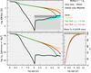 |
Fig. A.1 upper panel: predicted EW(Hα) (Å) as a function of time for a solar-metallicity stellar population with a Salpeter IMF forming instantaneously (black), continuously at a constant SFR (yellow), and with an exponentially decreasing SFR with e-folding times te of 1 Gyr and 3 Gyr (green and red curve, respectively). The light gray shaded area in the lower right part of the diagram encompasses the range in EW(Hα) predicted from pAGB photoionization for ages ≥0.1 Gyr, and the narrow dark strip depicts the corresponding prediction (EW(Hα) ≃ 1 Å ≡ ⟨ EW⋆ ⟩) for the typical age of ETGs (≥6 Gyr). The lower panel shows the time evolution of the Lyc photon rate expected by the instantaneous and exponentially decreasing SFR models, and the mass fraction in percent of stars older than 100 Myr (referred to as pAGB) is displayed separately in the lower right diagram. |
Figure A.1 shows the well-known fact (see, e.g., Leitherer et al. 1999; Weilbacher & Fritze-von Alvensleben 2001; Kotulla et al. 2009) that the Lyc photon rate and the corresponding Balmer-line EWs show a strong evolution with time, depending on the assumed SFH. For an instantaneous burst model, the Lyc photon rate (s-1), following a steep decrease by ~5 dex over the first 108 yr of galaxy evolution, decreases to a nearly constant level, scaling only with the available stellar mass as ≈1041ℳ⋆/M⊙ (see also Cid Fernandes et al. 2011). This results in a nearly constant EW(Hα) in the narrow range between ~0.1 Å and ~2.4 Å (EW) over nearly the whole Hubble time. We note that an EW(Hα) ≃ 0.1 Å corresponds to a short (<50 Myr) period at the onset of the pAGB phase. As the curves within the shaded area of Fig. A.1 depict, the EW(Hα) predicted for the pure pAGB component for other SFHs also shows little evolution with time, with the notable trend, however, of remaining lower than predicted for the instantaneous burst model. This is particularly true for the continuous SF model, which implies for the EW(Hα), owing to the pAGB component alone, a value lower by a factor ~2 than the single-burst model. However, by considering that the EW(Hα) is expected to arise from the total (young+pAGB) stellar component (curves in the upper part of the same panel), it is obvious that continuous as well as exponentially decreasing (te = 3 Gyr) SF models can be discarded for ETGs, as they predict a large (≥6 Å) EW(Hα) even for an age of ~10 Gyr, whereas the observations (cf., e.g., P13 and Sect. 4) indicate values in the range of 1–2 Å. On the other hand, a model involving a shorter (te = 1 Gyr) phase of exponentially declining SFR (green curve) is compatible with the literature data, as it predicts an  after 6.3 Gyr of galactic evolution, just like the instantaneous SF model. For reasonable assumptions on the age of ETGs (≥6 Gyr), these last two SFHs consistently imply a narrow span between ~1 Å (⟨ EW⋆ ⟩) and EW for the EW(Hα) of photoionized gas. Allowing for a generous low limit of
  Å (corresponding to a minimum τ = 2 defined in P13 as a conservative low limit for the presence of Lyc escape), we consider an observed EW(Hα) in the range between 0.5 Å and 2.4 Å to be consistent with the pAGB photoionization hypothesis.
Appendix B: Analysis methodology
Figure B.1 provides a schematic overview of the three main modules of Porto3D (v.2), which are briefly described next.
 |
Fig. B.1 Schematic outline of the three main modules of Porto3D (v.2). |
Appendix B.1: Module m.1: Computation of stellar fits and post-processing of the results
The module m.1, which is invoked at the first stage, extracts spectra from an IFS cube spaxel by spaxel, along with auxiliary information provided by the CALIFA data reduction pipeline (error spectrum, bad pixel map), computes initial statistics, and performs a number of preparatory steps that are necessary for subsequent fitting with Starlight. These include the computation of the signal-to-noise (S/N) in various spectral windows (with the option of rejecting spaxels that do not satisfy certain quality criteria), the flagging of spurious features and emission lines within pre-defined or automatically generated spectral masks, and the spectral resampling to the restframe and wavelength rebinning to 1 Å/pixel. The observed flux at each wavelength Oλ and its uncertainty eλ, provided by the CALIFA v1.3c reduction pipeline output or auto-computed with a sliding boxcar filter4, are finally exported together with flagging tags into ascii files in the format required for subsequent fitting with Starlight. This module also creates up to 16 execution scripts, facilitating automated parallel spectral fitting of the data with multicore CPUs. For each sample galaxy, typically ~2700 individual spectra with a S/N ≳ 30 at the normalization wavelength (5150 Å) were extracted and modeled with Starlight.
The goal of Starlight is decomposing an observed spectrum into a linear combination of its constituent SSP spectra. A description of the code is given in Cid Fernandes et al. (2005, C05, 2007); and subsequent publications of the SEAGal collaboration5 and is supplemented by a detailed cookbook for its application.
The best-fitting set of SSPs, together with the derived intrinsic V band extinction and velocity dispersion of the stellar component, are referred to in the following as the population vector. This encapsulates all information of the best-fitting model spectrum Mλ![Mathematical equation: \appendix \setcounter{section}{2} \begin{equation} M_\lambda =M_{\lambda_0} \left[ \sum\limits_{j=1}^{N_\star} x_j~b_{j,\lambda}~r_\lambda \right] \otimes G(v_\star,\sigma_\star), \end{equation}](/articles/aa/full_html/2016/04/aa25976-15/aa25976-15-eq143.png) (B.1)where
(B.1)where  is the spectrum of the jth SSP normalized at λ0, rλ ≡ 10− 0.4(Aλ−Aλ0) is the reddening term, x is the population vector, Mλ0 is the synthetic flux at the normalization wavelength, N⋆ is the total number of SSPs, G(v⋆,σ⋆) is the line-of-sight stellar velocity distribution, modeled as a Gaussian centered at velocity v⋆ and broadened by σ⋆.
The convergence of the solution is driven by the standard χ2 minimization with respect to the observed spectrum Oλ![Mathematical equation: \appendix \setcounter{section}{2} \begin{equation} \chi^2(x,M_{\lambda_0},A_V,v_\star,\sigma_\star) = \sum\limits_{\lambda=1}^{N_\lambda} \left[ \left(O_\lambda - M_\lambda \right) w_\lambda \right]^2, \end{equation}](/articles/aa/full_html/2016/04/aa25976-15/aa25976-15-eq155.png) (B.2)whereby spectral weights wλ are given by the inverse of the error spectrum eλ.
(B.2)whereby spectral weights wλ are given by the inverse of the error spectrum eλ.
Starlight fits were computed in the spectral region between 4000 Å and 6800 Å. This was mainly because the S/N of our sample ETGs blueward of 4000 Å is generally too low for a reliable stellar fit and the subsequent determination of the flux in the [Oii]λλ3726,3729 line doublet. The red spectral region (6900–7300 Å) was also disregarded because of its generally low S/N and spectral artifacts that are due to vignetting in the outer part of the PPAK FOV (see Sánchez et al. 2012).
 |
Fig. B.2 a) Example of a high-quality fit with Starlight to a V500 spectrum (blue and orange, respectively) extracted from an off-nucleus spaxel of the ETG NGC 5966. From the lower left panel b) it is apparent that the fit residuals are small (on average, ≲5% of the stellar continuum level) but systematic (see also Fig. B.4 and discussion in Appendix B.2). Shaded areas depict wavelength intervals that were flagged before spectral fitting. Panels c) and d) display the luminosity (xj) and mass (μj) contribution of individual SSPs (1 ...j) in the best-fitting population vector. The thin gray vertical lines in the upper right panel depict the 34 ages available in the SSP library for three stellar metallicities (color coded), and the shaded area in the lower panel shows a smoothed version of the μj, which is meant as an illustration of the star formation history. The fit implies a dominant old (pAGB) stellar population that has suffered little intrinsic extinction (AV ≲ 0.2 mag). |
For each spaxel Starlight fits employing between 7 and 12 Markov chains were computed twice, using two different simple stellar population (SSP) libraries, each comprising 34 ages (between 5 Myr and 13 Gyr) and three metallicities (0.008, 0.019, 0.03), that is, 102 SSPs in total. The first set of models uses SSPs from Bruzual & Charlot (2003, hereafter BC03). As these cover the UV spectral range, they allow inferring the Lyc photon output from each best-fitting population vector (see Appendix A for further details), which is in turn used to compute the τ ratio (module m.3). For the second set of Starlight fits we used SSPs from MILES (Sánchez-Blázquez et al. 2006; Vazdekis et al. 2010; Falcón-Barroso et al. 2011), which only cover the optical spectral range (3540–7410 Å).
The module m.1 also permits spaxel binning before fitting according to various prescriptions (e.g., averaging to a constant S/N along azimuthal segments within isophotal annuli, see discussion in Appendix B.4 and Fig. B.5). While a number of parallel runs on binned data cubes were conducted to check that the detection of faint nebular emission in the extranuclear component of our sample ETGs was reliable, we resorted to the method used in K12 and P13 of carrying the spectral analysis in a single-spaxel (sisp) mode and subsequently combining the results within irregular annuli (Appendix B.4).
Figure B.2 shows a high-quality (mean percentual deviation ADEV ≃ 1.4; cf. Starlight manual and Cid Fernandes et al. 2005) fit to a high-S/N spectrum from an off-center spaxel in the ETG NGC 5966. The observed spectrum Oλ, normalized at 5150 Å, and the fit (Mλ) to it are shown in orange and blue, respectively, in panel a. The lower left panel b displays the fit residuals, with shaded regions depicting spectral regions flagged before the fit, or subsequently rejected by Starlight. Panels c and d show the luminosity (xj) and mass (μj) contribution of the individual SSPs (1 ...j) composing the best-fitting population vector. The thin gray vertical lines in the upper right panel indicate the 34 ages available in the SSP library for the three stellar metallicities (each coded by a different color), and the shaded area in the lower panel shows a smoothed version of the μj distribution. The latter represents an illustrative approximation to the true SFH of stellar populations within the spaxel under study. The SFH clearly involves an extended star formation episode occurring until ~7 Gyr ago with a recent SF peak at ~10 Myr. This fit therefore indicates that the stellar mass ℳ⋆ is dominated by an evolved pAGB stellar population with a mass-weighted age of 8.2 Gyr. It also implies little intrinsic extinction (≲0.2 V mag) and no significant star-forming activity over the past ~1 Gyr.
The module m.1, besides storing the relevant output from each fit (σ⋆, v⋆, ..., among others), computes various quantities of interest, such as the time at which 50% of the present-day and ever-formed ℳ⋆ was in place, the luminosity contribution of stars formed in the past 5 Gyr (ℳ⋆,5 Gyr), and the luminosity- and mass-weighted mean stellar age (⟨t⋆⟩L and ⟨t⋆⟩M, respectively) as  (B.3)and
  (B.4)The dispersion of these quantities is also computed in the standard manner and exported into a data cube with dimension x × y × z, where x × y is the dimension of the CALIFA input IFS cubes in arcsec and z holds various quantities (age, metallicity, kinematics, emission-line fluxes, etc.) for each spaxel.
The ⟨ t⋆ ⟩ ℳ and ℳ⋆,5 Gyr maps provided by Porto3D (see Fig. B.3 for an example) were only used to check the soundness of the Starlight fits and checking the pAGB nature of the stellar component in the studied ETGs.
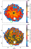 |
Fig. B.3 Luminosity-weighted and mass-weighted stellar age (upper and lower map, respectively) in Gyr (right-hand vertical bar) determined from Starlight fits to individual spaxels. A trend for decreasing age with radius is apparent, in qualitative agreement with the results by González Delgado et al. (2014a). The ⟨ t⋆ ⟩ ℳ map indicates a mass-weighted stellar age of ≥7 Gyr throughout the optical extent of the ETG. |
Appendix B.2: Module m.2: Computation of emission-line maps
The extraction of emission-line fluxes in ETGs is in itself a challenging task because of their faintness, as already pointed out in several previous studies (e.g., Sarzi et al. 2006; Annibali et al. 2010; K2; P13). Indeed, faint (EW ~ 1 Å) emission lines, buried within broader stellar absorption features, can only be detected and quantitatively studied upon precise subtraction of a high-S/N stellar continuum. Even in this case, a careful assessment of their uncertainties in individual spaxels is fundamental.
Previous longslit and IFS studies have generally investigated the diffuse wim component of ETGs down to EW levels of ≳2 Å, that is, of the order of the EWs of Balmer stellar absorption profiles, leading to the conclusion that two thirds of ETGs show faint nuclear and extranuclear nebular emission. A key contribution to advancing our understanding of the wim component in ETGs has been made by the SAURON project, which has first disclosed the diversity of emission-line morphologies and kinematics in these systems. Quite importantly, Sarzi et al. (2006) reported the detection of very faint (EW ~ 0.1 Å) Hβ emission in some ETGs, showing that even systems that were previously thought to be entirely devoid of ionized gas actually contain a low surface brightness substrate of wim.
It is important to bear in mind, on the other hand, that emission-line flux determinations in ETGs are sensitively dependent on the quality of stellar fits, which in many cases show subtle but systematic residuals. An example is given in Fig. B.4, where we show a typical, moderate-quality fit to a sisp high-S/N spectrum. The upper panel shows that fitting residuals are minor (on average, ≤5% of the normalized continuum), but systematic with both narrow (~40 Å) and broader (~200 Å) spectral intervals imperfectly fitted. These residuals were discussed, for instance, in (Sarzi et al. 2006; Walcher et al. 2006) and were ascribed to a combination of various causes (e.g., imperfections in SSPs and/or fitting codes, α element enhancement, and contamination from telluric line emission). In the framework of CALIFA, this problem was further analyzed in Husemann et al. (2013) through median-averaging of several thousands of individual spectra, showing indeed a systematic behavior in the residuals, in agreement with a parallel study by our team. The latter has shown that broad ripples in fitting residuals are partly due to inaccuracies in the spectral sensitivity function adopted in the CALIFA v1.3c reduction pipeline. Indeed, a reprocessing with Porto3D of part of the IFS data after reduction with the upgraded version v1.4 shows that these broad residuals are much reduced or absent, although smaller scale residuals generally persist. This problem is currently under scrutiny within the CALIFA collaboration.
On the other hand, as pointed out in Husemann et al. (2013), since these residuals are on the order of or lower than the continuum noise level, their effect on emission-line determinations is in practice negligible. While we concur with this statement, based on the analysis of a few emission-line galaxies in our comparison sample (see Appendix D), we find that small-scale fitting residuals can significantly affect flux determinations for faint (EW ~ 1 Å) emission lines when the standard technique of approximating the local rest-continuum by a first-order polynomial is used. In this case, Gaussian line fitting or deblending may fail to converge, or could lead to large errors owing to small-scale variations of the local background below and adjacent to emission lines. For this reason, these systematic fitting residuals could effectively place an EW limit of >2 Å on studies of the wim, even when high-S/N spectra are available.
To alleviate this problem, Porto3D performs for each sisp a rectification of the rest-continuum (i.e., Oλ–Mλ), which is based on an 1D adaptation of the flux-conserving unsharp masking technique by Papaderos et al. (1998). This approach permits determining a smooth version for the rest-continuum that is then subtracted from the input data array, yielding a net emission-line spectrum with a mean value of zero unless emission lines are present (cf. lower panel of Fig. B.4). Other than the more conventional approach of refitting the residual continuum with a high-order polynomial, this technique captures and corrects both for large- and small-scale fitting residuals, while leaving noise statistics unaffected.
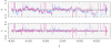 |
Fig. B.4 Upper panel: subtraction of the best-fitting stellar SED computed with Starlight with two different SSP libraries (BC03 and MILES; blue and magenta, respectively) from an observed sisp spectrum extracted from an off-nucleus region of a CALIFA ETG. The fit residuals are comparatively small, on the order of 1–2σ of the continuum in the blue spectral range, but they are systematic. lower panel: the same spectrum after rectification of the rest-continuum. |
The determination of emission-line fluxes from rectified net spectra is based on the combined application of two methods. The first one (el1) employs standard Gaussian line fitting or deblending with the Levenberg-Marquardt nonlinear fitting algorithm, and the second (el2) is a simple summation of the flux within predefined spectral windows centered on the laboratory wavelength of up to 50 emission lines, after correction for local motions. In the first case, the previous rectification of the residual continuum to a zero level is a key advantage, facilitating fast convergence and enhancing the robustness of emission-line measurements, thereby permitting an extension of the analysis down to EWs ~ 0.5 Å for a typical S/N ≳ 50 in the continuum. This is largely because the continuum rectification effectively eliminates two free parameters (level and slope of the local continuum) in fitting or deblending. In cases where the deblending of the Hα line from the [Nii] lines has failed to converge into a sensible solution, for example, the [Nii]λ6584/Hα ratio deviates from ~3 beyond certain tolerance bounds, el1 switches to a coarse determination of the Hα flux by fitting the [Nii]λ6584 line alone and by assuming a [Nii]λ6584/[Nii]λ6548 = 3. Before applying meth. el2, Porto3D uses the gas kinematics pattern inferred from el1 to slightly adjust the center of the spectral windows [λmin:λmax] within which the flux summation is performed.
 |
Fig. B.5 Adaptation of the irregular annuli surface photometry technique by Papaderos et al. (2002) for the purpose of azimuthal binning of spaxels to a constant S/N within radial zones. The color coding is meant to illustrate the segmentation within isophotal annuli. |
Porto3D (v.2) estimates uncertainties in line fluxes by considering in quadrature four contributions to the error budget. The first – only taken into account for el1 measurements - reflects formal errors in the fit as obtained from the covariance matrix and is negligible in most cases. The second term considers photon statistics following a widely used formula (e.g., Gonzáles-Delgado et al. 1995; Castellanos et al. 2002, see also K12), 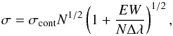 (B.5)where σcont is the uncertainty in the determination of the local continuum (defined by its noise level), N the width of the region used to measure the line in pixels, Δλ the spectral dispersion in Å pix-1, and EW the equivalent width of the line in Å.
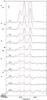 |
Fig. B.6 Integrated spectra of the type i ETG NGC 1167a) and the type ii ETGs NGC 6338 and NGC 7550 (panels b) and c), respectively) within successive isophotal annuli (isan), after subtracting the stellar emission and rectifying the continuum. Each spectrum is labeled with the photometric radius (′′) of the annulus within which it was sampled and is vertically shifted by an arbitrary amount, with the overlaid dotted horizontal lines depicting the zero level. The vertical bar in each panel corresponds to a flux level interval of 10-16 erg s-1 cm-2. The extreme faintness of extended nebular emission in type ii ETGs, as compared to the type i ETG NGC 1167, is apparent. |
Emission-line EWs were computed from the ratio between the line flux (measured on the net emission-line spectra) and the rectified model SED (Mλ). The third term, which is only included in el2 measurements, uses the noise distribution array in connection with an empirical scaling factor to gauge how the line flux registered within the spectral window considered could be affected by positive and negative photon noise peaks at the 1σ level. We note that none of the above terms captures uncertainties related to the quality of the stellar fitting. An analytical estimate for the latter is obviously a non-trivial task, given that it also has to include a realistic description of how errors in the best-fitting stellar velocity dispersion, and stellar metallicity may affect fluxes of emission lines that are embedded within broader stellar absorption features. As a remedy to this problem, Porto3D includes for el2 measurements an error contribution that is linked to the local deviation δfit of the fit (i.e., the value of the rectification array within the respective spectral window δλ) as 0.68·δλ· | δfit |. This term, which typically dominates for faint emission-line fluxes, admittedly simplistic, is meant as a minimum attempt to quantify the cumulative impact of systematic errors in spectral fits on the recovered emission-line fluxes. Related to this issue is most likely also the quality of the SSP models adopted. As we pointed out in K12, the fluxes of faint (EW(Hα) ≲ 1 Å) emission lines in ETGs may change by to up to 10% depending on whether BC03 or MILES SSPs are used. For this reason, we have taken in this and our previous studies the computationally expensive approach of performing the full IFS data processing (spectral fitting and determining emission lines) twice, both with the BC03 and MILES SSP library, and to subsequently combine the results. This was done with a decision-tree routine that prioritizes the up to four determinations for each spaxel (el1 and el2 for two SSP libraries) according to their soundness and estimated uncertainties. This procedure uses an initial sanity check of several quantities (errors, FWHM of emission lines, and in the case of the Hα+[Nii] blend, the difference between their central wavelengths) and, in a second pass, the [Nii] 6584/6548 ratios. Preference was generally given to el1 determinations, which, whenever available for both BC- and MILES-based fits, were error-weighted averaged. When only one determination passed the quality check, it was adopted for the final map, and the same decision procedure was followed for el2 measurements, which were typically used in low-S/N, low-EW(Hα) spectra.
Appendix B.3: Module m.3: Computation of the τ ratio
The τ ratio, defined in K12 as the ratio of the Balmer-line luminosity expected to arise from pure pAGB photoionization to the observed one, offers a simple but efficient means for assessing whether or not hot pAGB stars are capable of powering the extended wim in ETGs. After our pilot analysis of the radial distribution of τ in two ETGs (K12), we extended this analysis in P13 to the present sample of 32 ETGs to test the pAGB photoionization hypothesis.
Porto3D includes a routine that determines the total Lyc photon output for each Starlight fit by integrating shortward of the Lyc edge of the UV continuum the SEDs of the individual SSPs (BC) that compose the best-fitting population vector. In this procedure, only SSPs for stellar populations older than 108 yr are considered so that we only compute the total Lyc output of the pAGB component. The Balmer-line luminosities expected from it are computed assuming case B recombination and standard conditions for the gas (ne = 100 cm-3, Te = 10 000 K). In ETGs, the typically large uncertainties in emission-line fluxes and their ratios generally prevent a reliable determination of the intrinsic extinction in the wim. Therefore, the optional inclusion of intrinsic extinction in Porto3D m.3 has to rely on the stellar V band extinction, as inferred from Starlight fits, which was generally found to be low (<0.1 mag).
As discussed in our previous studies (see also Sect. 1), a τ ≃ 1 corresponds to an equilibrium situation where the Lyc photon rate from pAGB stars precisely balances the observed Hα luminosity. A τ< 1, on the other hand, indicates an additional contribution by an extra source, such as AGN, shocks or OB stars. Finally, as we discussed in P13, a τ ratio exceeding unity corresponds to the situation of leakage of a fraction 1−τ-1 of the Lyc output from the pAGB component. However, given the inherent uncertainties in the currently available model predictions for the UV output from pAGB stars, we conservatively assumed a τ ≥ 2 as robust evidence for Lyc escape in P13 and in this study.
Appendix B.4: Computation of radial profiles
In Sect. 4 we showed the radial distribution of various quantities of interest, such as the intensity and EW of the Hα emission line, and the [O iii]5007/Hβ, [N ii]6584/Hα and τ ratios. Following the method used in P13, we included two complementary data sets in all diagrams:
-
i)
single-spaxel (sisp) determinations from fits with an ADEV | Oλ−Mλ | / Oλ ≤ 2.6 (cf.K12 and the Starlight manual). This higher-S/Nsubsample has the lowest uncertainties in fitting parameters, andemission-line fluxes at the price of being spatially restricted totypically the central, higher surface brightness part(μ ≲ 23 g mag/Λ″) of the studied galaxies.
-
ii)
The average of all sisp determinations within isophotal annuli (isan) adapted to the morphology of the (line-free) continuum between 6390 Å and 6490 Å. These data, which are to be considered in a statistical sense, reach ≳2 mag fainter, allowing the study of the wim in the ETG periphery.
The isophotal annuli method (Papaderos et al. 2002, referred to as meth. iv; subsequently as Lazy by Noeske et al. 2003, 2006) was developed with the goal of deriving radial surface brightness and nebular line intensity profiles in irregular galaxies with a poorly constrained optical center, for which the conventional approach of fitting ellipses to isophotes of 2D axis-symmetric luminosity components is of limited applicability. Its main concept consists of determining photon statistics within equidistant logarithmic slices of a galaxy image (or of a reference image, such as a stacked image of all available passbands, or in the context of this study, the line-free 6390–6490 Å pseudo-continuum image), with each of these irregular slices faithfully reproducing the morphology of a galaxy within each intensity interval [I:I+δI] and corresponding to a well-defined photometric radius R⋆. In the context of IFS data, this technique was first used in K12 (see their appendix for further details) and more recently by Sánchez et al. (2014b) to derive gas-phase metallicity gradients in CALIFA late-type galaxies.
Figure B.5 illustrates the adaptation of the isophotal annuli technique so that azimuthal binning of spaxels to a constant S/N within radial zones is permitted. This add-on routine to Porto3D was used in P13 and in this study to double-check the presence of extended nebular emission in ETGs. These tests were supplemented by modeling the integrated spectrum within each annulus, extracted by the same routine by requesting an unrealistically high S/N. Figure B.6 shows examples of the residual emission after subtracting the stellar fit with BC SSPs and continuum rectification within successively larger annuli for three ETGs from our sample, illustrating that nebular emission in type ii ETGs (NGC 6338 and NGC 7550; panels b and c) is fainter than in type i ETGs (NGC 1167; panel a).
Appendix C: 2D emission-line patterns and kinematics for 32 galaxies
This section illustrates the diversity of ETG galaxies within our sample with respect to morphology, kinematics, and physical properties of their warm interstellar medium. The galaxies are ordered as in Table 1. We note that the maps and radial profiles (a–n) follow the same definitions and colors as in Sect. 4.
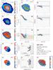 |
Fig. C.1 UGC 5771: 2D maps (panels a)–f) and n)), radial intensity and EW of Hα (panels g) and h)), BPT diagrams (panels i) and j)), radial distribution of diagnostic line ratios (k) and l)), and the τ ratio (panel m)). In all 2D maps north is up and east to the left. The bar corresponds to 20′′. |
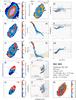 |
Fig. C.2 NGC 4003: 2D maps (panels a)–f) and n)), radial intensity and EW of Hα (panels g) and h)), BPT diagrams (panels i) and j)), radial distribution of diagnostic line ratios (k) and l)), and the τ ratio (panel m)). In all 2D maps north is up and east to the left. The bar corresponds to 20′′. |
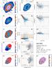 |
Fig. C.3 UGC 8234: 2D maps (panels a)–f) and n)), radial intensity and EW of Hα (panels g) and h)), BPT diagrams (panels i) and j)), radial distribution of diagnostic line ratios (k) and l)), and the τ ratio (panel m)). In all 2D maps north is up and east to the left. The bar corresponds to 20′′. |
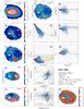 |
Fig. C.4 NGC 5966: 2D maps (panels a)–f) and n)), radial intensity and EW of Hα (panels g) and h)), BPT diagrams (panels i) and j)), radial distribution of diagnostic line ratios (k) and l)), and the τ ratio (panel m)). In all 2D maps north is up and east to the left. The bar corresponds to 20′′. |
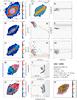 |
Fig. C.5 UGC 10205: 2D maps (panels a)–f) and n)), radial intensity and EW of Hα (panels g) and h)), BPT diagrams (panels i) and j)), radial distribution of diagnostic line ratios (k) and l)), and the τ ratio (panel m)). In all 2D maps north is up and east to the left. The bar corresponds to 20′′. |
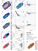 |
Fig. C.6 NGC 6081: 2D maps (panels a)–f) and n)), radial intensity and EW of Hα (panels g) and h)), BPT diagrams (panels i) and j)), radial distribution of diagnostic line ratios (k) and l)), and the τ ratio (panel m)). In all 2D maps north is up and east to the left. The bar corresponds to 20′′. |
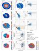 |
Fig. C.7 NGC 6146: 2D maps (panels a)–f) and n)), radial intensity and EW of Hα (panels g) and h)), BPT diagrams (panels i) and j)), radial distribution of diagnostic line ratios (k) and l)), and the τ ratio (panel m)). In all 2D maps north is up and east to the left. The bar corresponds to 20′′. |
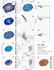 |
Fig. C.8 UGC 10695: 2D maps (panels a)–f) and n)), radial intensity and EW of Hα (panels g) and h)), BPT diagrams (panels i) and j)), radial distribution of diagnostic line ratios (k) and l)), and the τ ratio (panel m)). In all 2D maps north is up and east to the left. The bar corresponds to 20′′. |
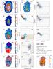 |
Fig. C.9 UGC 10905: 2D maps (panels a)–f) and n)), radial intensity and EW of Hα (panels g) and h)), BPT diagrams (panels i) and j)), radial distribution of diagnostic line ratios (k) and l)), and the τ ratio (panel m)). In all 2D maps north is up and east to the left. The bar corresponds to 20′′. |
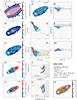 |
Fig. C.10 NGC 6762: 2D maps (panels a)–f) and n)), radial intensity and EW of Hα (panels g) and h)), BPT diagrams (panels i) and j)), radial distribution of diagnostic line ratios (k) and l)), and the τ ratio (panel m)). In all 2D maps north is up and east to the left. The bar corresponds to 20′′. |
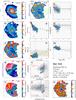 |
Fig. C.11 NGC 7025: 2D maps (panels a)–f) and n)), radial intensity and EW of Hα (panels g) and h)), BPT diagrams (panels i) and j)), radial distribution of diagnostic line ratios (k) and l)), and the τ ratio (panel m)). In all 2D maps north is up and east to the left. The bar corresponds to 20′′. |
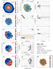 |
Fig. C.12 NGC 1349: 2D maps (panels a)–f) and n)), radial intensity and EW of Hα (panels g) and h)), BPT diagrams (panels i) and j)), radial distribution of diagnostic line ratios (k) and l)), and the τ ratio (panel m)). In all 2D maps north is up and east to the left. The bar corresponds to 20′′. |
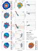 |
Fig. C.13 NGC 3106: 2D maps (panels a)–f) and n)), radial intensity and EW of Hα (panels g) and h)), BPT diagrams (panels i) and j)), radial distribution of diagnostic line ratios (k) and l)), and the τ ratio (panel m)). In all 2D maps north is up and east to the left. The bar corresponds to 20′′. |
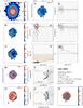 |
Fig. C.14 UGC 0029: 2D maps (panels a)–f) and n)), radial intensity and EW of Hα (panels g) and h)), BPT diagrams (panels i) and j)), radial distribution of diagnostic line ratios (k) and l)), and the τ ratio (panel m)). In all 2D maps north is up and east to the left. The bar corresponds to 20′′. |
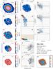 |
Fig. C.15 NGC 2918: 2D maps (panels a)–f) and n)), radial intensity and EW of Hα (panels g) and h)), BPT diagrams (panels i) and j)), radial distribution of diagnostic line ratios (k) and l)), and the τ ratio (panel m)). In all 2D maps north is up and east to the left. The bar corresponds to 20′′. |
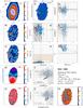 |
Fig. C.16 NGC 3300: 2D maps (panels a)–f) and n)), radial intensity and EW of Hα (panels g) and h)), BPT diagrams (panels i) and j)), radial distribution of diagnostic line ratios (k) and l)), and the τ ratio (panel m)). In all 2D maps north is up and east to the left. The bar corresponds to 20′′. |
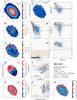 |
Fig. C.17 NGC 3615: 2D maps (panels a)–f) and n)), radial intensity and EW of Hα (panels g) and h)), BPT diagrams (panels i) and j)), radial distribution of diagnostic line ratios (k) and l)), and the τ ratio (panel m)). In all 2D maps north is up and east to the left. The bar corresponds to 20′′. |
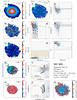 |
Fig. C.18 NGC 4816: 2D maps (panels a)–f) and n)), radial intensity and EW of Hα (panels g) and h)), BPT diagrams (panels i) and j)), radial distribution of diagnostic line ratios (k) and l)), and the τ ratio (panel m)). In all 2D maps north is up and east to the left. The bar corresponds to 20′′. |
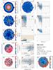 |
Fig. C.19 NGC 6125: 2D maps (panels a)–f) and n)), radial intensity and EW of Hα (panels g) and h)), BPT diagrams (panels i) and j)), radial distribution of diagnostic line ratios (k) and l)), and the τ ratio (panel m)). In all 2D maps north is up and east to the left. The bar corresponds to 20′′. |
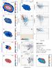 |
Fig. C.20 NGC 6150: 2D maps (panels a)–f) and n)), radial intensity and EW of Hα (panels g) and h)), BPT diagrams (panels i) and j)), radial distribution of diagnostic line ratios (k) and l)), and the τ ratio (panel m)). In all 2D maps north is up and east to the left. The bar corresponds to 20′′. |
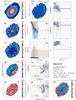 |
Fig. C.21 NGC 6173: 2D maps (panels a)–f) and n)), radial intensity and EW of Hα (panels g) and h)), BPT diagrams (panels i) and j)), radial distribution of diagnostic line ratios (k) and l)), and the τ ratio (panel m)). In all 2D maps north is up and east to the left. The bar corresponds to 20′′. |
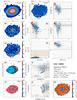 |
Fig. C.22 UGC 10693: 2D maps (panels a)–f) and n)), radial intensity and EW of Hα (panels g) and h)), BPT diagrams (panels i) and j)), radial distribution of diagnostic line ratios (k) and l)), and the τ ratio (panel m)). In all 2D maps north is up and east to the left. The bar corresponds to 20′′. |
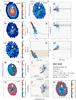 |
Fig. C.23 NGC 6338: 2D maps (panels a)–f) and n)), radial intensity and EW of Hα (panels g) and h)), BPT diagrams (panels i) and j)), radial distribution of diagnostic line ratios (k) and l)), and the τ ratio (panel m)). In all 2D maps north is up and east to the left. The bar corresponds to 20′′. |
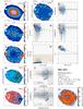 |
Fig. C.24 NGC 6411: 2D maps (panels a)–f) and n)), radial intensity and EW of Hα (panels g) and h)), BPT diagrams (panels i) and j)), radial distribution of diagnostic line ratios (k) and l)), and the τ ratio (panel m)). In all 2D maps north is up and east to the left. The bar corresponds to 20′′. |
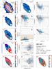 |
Fig. C.25 NGC 6427: 2D maps (panels a)–f) and n)), radial intensity and EW of Hα (panels g) and h)), BPT diagrams (panels i) and j)), radial distribution of diagnostic line ratios (k) and l)), and the τ ratio (panel m)). In all 2D maps north is up and east to the left. The bar corresponds to 20′′. |
 |
Fig. C.26 NGC 6515: 2D maps (panels a)–f) and n)), radial intensity and EW of Hα (panels g) and h)), BPT diagrams (panels i) and j)), radial distribution of diagnostic line ratios (k) and l)), and the τ ratio (panel m)). In all 2D maps north is up and east to the left. The bar corresponds to 20′′. |
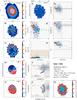 |
Fig. C.27 NGC 7194: 2D maps (panels a)–f) and n)), radial intensity and EW of Hα (panels g) and h)), BPT diagrams (panels i) and j)), radial distribution of diagnostic line ratios (k) and l)), and the τ ratio (panel m)). In all 2D maps north is up and east to the left. The bar corresponds to 20′′. |
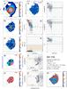 |
Fig. C.28 NGC 7236: 2D maps (panels a)–f) and n)), radial intensity and EW of Hα (panels g) and h)), BPT diagrams (panels i) and j)), radial distribution of diagnostic line ratios (k) and l)), and the τ ratio (panel m)). In all 2D maps north is up and east to the left. The bar corresponds to 20′′. |
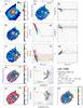 |
Fig. C.29 UGC 11958: 2D maps (panels a)–f) and n)), radial intensity and EW of Hα (panels g) and h)), BPT diagrams (panels i) and j)), radial distribution of diagnostic line ratios (k) and l)), and the τ ratio (panel m)). In all 2D maps north is up and east to the left. The bar corresponds to 20′′. |
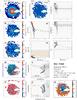 |
Fig. C.30 NGC 7436B: 2D maps (panels a)–f) and n)), radial intensity and EW of Hα (panels g) and h)), BPT diagrams (panels i) and j)), radial distribution of diagnostic line ratios (k) and l)), and the τ ratio (panel m)). In all 2D maps north is up and east to the left. The bar corresponds to 20′′. |
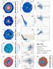 |
Fig. C.31 NGC 7550: 2D maps (panels a)–f) and n)), radial intensity and EW of Hα (panels g) and h)), BPT diagrams (panels i) and j)), radial distribution of diagnostic line ratios (k) and l)), and the τ ratio (panel m)). In all 2D maps north is up and east to the left. The bar corresponds to 20′′. |
Appendix D: Comparison with star-forming and composite galaxies
This appendix is meant to illustrate the variation of the EW(Hα), τ; and diagnostic line ratios from early- to late-type galaxies. All but one of these systems are classifiable by BPT ratios in their central part and/or an extranuclear component as composite or SF-dominated.
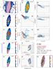 |
Fig. D.1 IC 0540: 2D maps (panels a)–f) and n)), radial intensity and EW of Hα (panels g) and h)), BPT diagrams (panels i) and j)), radial distribution of diagnostic line ratios (k) and l)), and the τ ratio (panel m)). In all 2D maps north is up and east to the left. The bar corresponds to 20′′. |
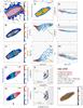 |
Fig. D.2 UGC 8778: 2D maps (panels a)–f) and n)), radial intensity and EW of Hα (panels g) and h)), BPT diagrams (panels i) and j)), radial distribution of diagnostic line ratios (k) and l)), and the τ ratio (panel m)). In all 2D maps north is up and east to the left. The bar corresponds to 20′′. |
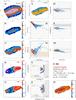 |
Fig. D.3 IC 0944: 2D maps (panels a)–f) and n)), radial intensity and EW of Hα (panels g) and h)), BPT diagrams (panels i) and j)), radial distribution of diagnostic line ratios (k) and l)), and the τ ratio (panel m)). In all 2D maps north is up and east to the left. The bar corresponds to 20′′. |
 |
Fig. D.4 IC 1683: 2D maps (panels a)–f) and n)), radial intensity and EW of Hα (panels g) and h)), BPT diagrams (panels i) and j)), radial distribution of diagnostic line ratios (k) and l)), and the τ ratio (panel m)). In all 2D maps north is up and east to the left. The bar corresponds to 20′′. |
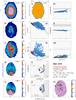 |
Fig. D.5 NGC 4470: 2D maps (panels a)–f) and n)), radial intensity and EW of Hα (panels g) and h)), BPT diagrams (panels i) and j)), radial distribution of diagnostic line ratios (k) and l)), and the τ ratio (panel m)). In all 2D maps north is up and east to the left. The bar corresponds to 20′′. |
All Tables
All Figures
|
Fig. 1 NGC 1167: 2D maps (panels a)–f) and n)), radial intensity and EW of Hα (panels g) and h)), BPT diagrams (panels i) and j)), radial distribution of diagnostic line ratios (k) and l)), and the τ ratio (panel m)). In all 2D maps north is up and east to the left. The bar corresponds to 20′′. |
| In the text | |
|
Fig. 2 Schematic representation of the two main classes of ETGs, as defined in P13. The EW(Hα) profiles of type i ETGs (blue), such as NGC 1167, show in their extranuclear component (beyond the radius range depicted by the vertical shaded area; typically ~2 kpc in our sample) nearly constant values within the narrow range between EW |
| In the text | |
|
Fig. 3 Emission-line-free stellar continuum a), Hα flux in 10-16 erg s-1 cm-2b) and Hα+[Nii] line-of-sight velocity in km/s c) of the type i+ ETG NGC 160, as inferred from processing of CALIFA (v1.5) V500 with Porto3D. The overlaid contours delineate the EW(Hα) morphology of the galaxy and reach from 4 Å to 21 Å in steps of 3 Å. North is up and east to the left. |
| In the text | |
|
Fig. A.1 upper panel: predicted EW(Hα) (Å) as a function of time for a solar-metallicity stellar population with a Salpeter IMF forming instantaneously (black), continuously at a constant SFR (yellow), and with an exponentially decreasing SFR with e-folding times te of 1 Gyr and 3 Gyr (green and red curve, respectively). The light gray shaded area in the lower right part of the diagram encompasses the range in EW(Hα) predicted from pAGB photoionization for ages ≥0.1 Gyr, and the narrow dark strip depicts the corresponding prediction (EW(Hα) ≃ 1 Å ≡ ⟨ EW⋆ ⟩) for the typical age of ETGs (≥6 Gyr). The lower panel shows the time evolution of the Lyc photon rate expected by the instantaneous and exponentially decreasing SFR models, and the mass fraction in percent of stars older than 100 Myr (referred to as pAGB) is displayed separately in the lower right diagram. |
| In the text | |
|
Fig. B.1 Schematic outline of the three main modules of Porto3D (v.2). |
| In the text | |
|
Fig. B.2 a) Example of a high-quality fit with Starlight to a V500 spectrum (blue and orange, respectively) extracted from an off-nucleus spaxel of the ETG NGC 5966. From the lower left panel b) it is apparent that the fit residuals are small (on average, ≲5% of the stellar continuum level) but systematic (see also Fig. B.4 and discussion in Appendix B.2). Shaded areas depict wavelength intervals that were flagged before spectral fitting. Panels c) and d) display the luminosity (xj) and mass (μj) contribution of individual SSPs (1 ...j) in the best-fitting population vector. The thin gray vertical lines in the upper right panel depict the 34 ages available in the SSP library for three stellar metallicities (color coded), and the shaded area in the lower panel shows a smoothed version of the μj, which is meant as an illustration of the star formation history. The fit implies a dominant old (pAGB) stellar population that has suffered little intrinsic extinction (AV ≲ 0.2 mag). |
| In the text | |
|
Fig. B.3 Luminosity-weighted and mass-weighted stellar age (upper and lower map, respectively) in Gyr (right-hand vertical bar) determined from Starlight fits to individual spaxels. A trend for decreasing age with radius is apparent, in qualitative agreement with the results by González Delgado et al. (2014a). The ⟨ t⋆ ⟩ ℳ map indicates a mass-weighted stellar age of ≥7 Gyr throughout the optical extent of the ETG. |
| In the text | |
|
Fig. B.4 Upper panel: subtraction of the best-fitting stellar SED computed with Starlight with two different SSP libraries (BC03 and MILES; blue and magenta, respectively) from an observed sisp spectrum extracted from an off-nucleus region of a CALIFA ETG. The fit residuals are comparatively small, on the order of 1–2σ of the continuum in the blue spectral range, but they are systematic. lower panel: the same spectrum after rectification of the rest-continuum. |
| In the text | |
|
Fig. B.5 Adaptation of the irregular annuli surface photometry technique by Papaderos et al. (2002) for the purpose of azimuthal binning of spaxels to a constant S/N within radial zones. The color coding is meant to illustrate the segmentation within isophotal annuli. |
| In the text | |
|
Fig. B.6 Integrated spectra of the type i ETG NGC 1167a) and the type ii ETGs NGC 6338 and NGC 7550 (panels b) and c), respectively) within successive isophotal annuli (isan), after subtracting the stellar emission and rectifying the continuum. Each spectrum is labeled with the photometric radius (′′) of the annulus within which it was sampled and is vertically shifted by an arbitrary amount, with the overlaid dotted horizontal lines depicting the zero level. The vertical bar in each panel corresponds to a flux level interval of 10-16 erg s-1 cm-2. The extreme faintness of extended nebular emission in type ii ETGs, as compared to the type i ETG NGC 1167, is apparent. |
| In the text | |
|
Fig. C.1 UGC 5771: 2D maps (panels a)–f) and n)), radial intensity and EW of Hα (panels g) and h)), BPT diagrams (panels i) and j)), radial distribution of diagnostic line ratios (k) and l)), and the τ ratio (panel m)). In all 2D maps north is up and east to the left. The bar corresponds to 20′′. |
| In the text | |
|
Fig. C.2 NGC 4003: 2D maps (panels a)–f) and n)), radial intensity and EW of Hα (panels g) and h)), BPT diagrams (panels i) and j)), radial distribution of diagnostic line ratios (k) and l)), and the τ ratio (panel m)). In all 2D maps north is up and east to the left. The bar corresponds to 20′′. |
| In the text | |
|
Fig. C.3 UGC 8234: 2D maps (panels a)–f) and n)), radial intensity and EW of Hα (panels g) and h)), BPT diagrams (panels i) and j)), radial distribution of diagnostic line ratios (k) and l)), and the τ ratio (panel m)). In all 2D maps north is up and east to the left. The bar corresponds to 20′′. |
| In the text | |
|
Fig. C.4 NGC 5966: 2D maps (panels a)–f) and n)), radial intensity and EW of Hα (panels g) and h)), BPT diagrams (panels i) and j)), radial distribution of diagnostic line ratios (k) and l)), and the τ ratio (panel m)). In all 2D maps north is up and east to the left. The bar corresponds to 20′′. |
| In the text | |
|
Fig. C.5 UGC 10205: 2D maps (panels a)–f) and n)), radial intensity and EW of Hα (panels g) and h)), BPT diagrams (panels i) and j)), radial distribution of diagnostic line ratios (k) and l)), and the τ ratio (panel m)). In all 2D maps north is up and east to the left. The bar corresponds to 20′′. |
| In the text | |
|
Fig. C.6 NGC 6081: 2D maps (panels a)–f) and n)), radial intensity and EW of Hα (panels g) and h)), BPT diagrams (panels i) and j)), radial distribution of diagnostic line ratios (k) and l)), and the τ ratio (panel m)). In all 2D maps north is up and east to the left. The bar corresponds to 20′′. |
| In the text | |
|
Fig. C.7 NGC 6146: 2D maps (panels a)–f) and n)), radial intensity and EW of Hα (panels g) and h)), BPT diagrams (panels i) and j)), radial distribution of diagnostic line ratios (k) and l)), and the τ ratio (panel m)). In all 2D maps north is up and east to the left. The bar corresponds to 20′′. |
| In the text | |
|
Fig. C.8 UGC 10695: 2D maps (panels a)–f) and n)), radial intensity and EW of Hα (panels g) and h)), BPT diagrams (panels i) and j)), radial distribution of diagnostic line ratios (k) and l)), and the τ ratio (panel m)). In all 2D maps north is up and east to the left. The bar corresponds to 20′′. |
| In the text | |
|
Fig. C.9 UGC 10905: 2D maps (panels a)–f) and n)), radial intensity and EW of Hα (panels g) and h)), BPT diagrams (panels i) and j)), radial distribution of diagnostic line ratios (k) and l)), and the τ ratio (panel m)). In all 2D maps north is up and east to the left. The bar corresponds to 20′′. |
| In the text | |
|
Fig. C.10 NGC 6762: 2D maps (panels a)–f) and n)), radial intensity and EW of Hα (panels g) and h)), BPT diagrams (panels i) and j)), radial distribution of diagnostic line ratios (k) and l)), and the τ ratio (panel m)). In all 2D maps north is up and east to the left. The bar corresponds to 20′′. |
| In the text | |
|
Fig. C.11 NGC 7025: 2D maps (panels a)–f) and n)), radial intensity and EW of Hα (panels g) and h)), BPT diagrams (panels i) and j)), radial distribution of diagnostic line ratios (k) and l)), and the τ ratio (panel m)). In all 2D maps north is up and east to the left. The bar corresponds to 20′′. |
| In the text | |
|
Fig. C.12 NGC 1349: 2D maps (panels a)–f) and n)), radial intensity and EW of Hα (panels g) and h)), BPT diagrams (panels i) and j)), radial distribution of diagnostic line ratios (k) and l)), and the τ ratio (panel m)). In all 2D maps north is up and east to the left. The bar corresponds to 20′′. |
| In the text | |
|
Fig. C.13 NGC 3106: 2D maps (panels a)–f) and n)), radial intensity and EW of Hα (panels g) and h)), BPT diagrams (panels i) and j)), radial distribution of diagnostic line ratios (k) and l)), and the τ ratio (panel m)). In all 2D maps north is up and east to the left. The bar corresponds to 20′′. |
| In the text | |
|
Fig. C.14 UGC 0029: 2D maps (panels a)–f) and n)), radial intensity and EW of Hα (panels g) and h)), BPT diagrams (panels i) and j)), radial distribution of diagnostic line ratios (k) and l)), and the τ ratio (panel m)). In all 2D maps north is up and east to the left. The bar corresponds to 20′′. |
| In the text | |
|
Fig. C.15 NGC 2918: 2D maps (panels a)–f) and n)), radial intensity and EW of Hα (panels g) and h)), BPT diagrams (panels i) and j)), radial distribution of diagnostic line ratios (k) and l)), and the τ ratio (panel m)). In all 2D maps north is up and east to the left. The bar corresponds to 20′′. |
| In the text | |
|
Fig. C.16 NGC 3300: 2D maps (panels a)–f) and n)), radial intensity and EW of Hα (panels g) and h)), BPT diagrams (panels i) and j)), radial distribution of diagnostic line ratios (k) and l)), and the τ ratio (panel m)). In all 2D maps north is up and east to the left. The bar corresponds to 20′′. |
| In the text | |
|
Fig. C.17 NGC 3615: 2D maps (panels a)–f) and n)), radial intensity and EW of Hα (panels g) and h)), BPT diagrams (panels i) and j)), radial distribution of diagnostic line ratios (k) and l)), and the τ ratio (panel m)). In all 2D maps north is up and east to the left. The bar corresponds to 20′′. |
| In the text | |
|
Fig. C.18 NGC 4816: 2D maps (panels a)–f) and n)), radial intensity and EW of Hα (panels g) and h)), BPT diagrams (panels i) and j)), radial distribution of diagnostic line ratios (k) and l)), and the τ ratio (panel m)). In all 2D maps north is up and east to the left. The bar corresponds to 20′′. |
| In the text | |
|
Fig. C.19 NGC 6125: 2D maps (panels a)–f) and n)), radial intensity and EW of Hα (panels g) and h)), BPT diagrams (panels i) and j)), radial distribution of diagnostic line ratios (k) and l)), and the τ ratio (panel m)). In all 2D maps north is up and east to the left. The bar corresponds to 20′′. |
| In the text | |
|
Fig. C.20 NGC 6150: 2D maps (panels a)–f) and n)), radial intensity and EW of Hα (panels g) and h)), BPT diagrams (panels i) and j)), radial distribution of diagnostic line ratios (k) and l)), and the τ ratio (panel m)). In all 2D maps north is up and east to the left. The bar corresponds to 20′′. |
| In the text | |
|
Fig. C.21 NGC 6173: 2D maps (panels a)–f) and n)), radial intensity and EW of Hα (panels g) and h)), BPT diagrams (panels i) and j)), radial distribution of diagnostic line ratios (k) and l)), and the τ ratio (panel m)). In all 2D maps north is up and east to the left. The bar corresponds to 20′′. |
| In the text | |
|
Fig. C.22 UGC 10693: 2D maps (panels a)–f) and n)), radial intensity and EW of Hα (panels g) and h)), BPT diagrams (panels i) and j)), radial distribution of diagnostic line ratios (k) and l)), and the τ ratio (panel m)). In all 2D maps north is up and east to the left. The bar corresponds to 20′′. |
| In the text | |
|
Fig. C.23 NGC 6338: 2D maps (panels a)–f) and n)), radial intensity and EW of Hα (panels g) and h)), BPT diagrams (panels i) and j)), radial distribution of diagnostic line ratios (k) and l)), and the τ ratio (panel m)). In all 2D maps north is up and east to the left. The bar corresponds to 20′′. |
| In the text | |
|
Fig. C.24 NGC 6411: 2D maps (panels a)–f) and n)), radial intensity and EW of Hα (panels g) and h)), BPT diagrams (panels i) and j)), radial distribution of diagnostic line ratios (k) and l)), and the τ ratio (panel m)). In all 2D maps north is up and east to the left. The bar corresponds to 20′′. |
| In the text | |
|
Fig. C.25 NGC 6427: 2D maps (panels a)–f) and n)), radial intensity and EW of Hα (panels g) and h)), BPT diagrams (panels i) and j)), radial distribution of diagnostic line ratios (k) and l)), and the τ ratio (panel m)). In all 2D maps north is up and east to the left. The bar corresponds to 20′′. |
| In the text | |
|
Fig. C.26 NGC 6515: 2D maps (panels a)–f) and n)), radial intensity and EW of Hα (panels g) and h)), BPT diagrams (panels i) and j)), radial distribution of diagnostic line ratios (k) and l)), and the τ ratio (panel m)). In all 2D maps north is up and east to the left. The bar corresponds to 20′′. |
| In the text | |
|
Fig. C.27 NGC 7194: 2D maps (panels a)–f) and n)), radial intensity and EW of Hα (panels g) and h)), BPT diagrams (panels i) and j)), radial distribution of diagnostic line ratios (k) and l)), and the τ ratio (panel m)). In all 2D maps north is up and east to the left. The bar corresponds to 20′′. |
| In the text | |
|
Fig. C.28 NGC 7236: 2D maps (panels a)–f) and n)), radial intensity and EW of Hα (panels g) and h)), BPT diagrams (panels i) and j)), radial distribution of diagnostic line ratios (k) and l)), and the τ ratio (panel m)). In all 2D maps north is up and east to the left. The bar corresponds to 20′′. |
| In the text | |
|
Fig. C.29 UGC 11958: 2D maps (panels a)–f) and n)), radial intensity and EW of Hα (panels g) and h)), BPT diagrams (panels i) and j)), radial distribution of diagnostic line ratios (k) and l)), and the τ ratio (panel m)). In all 2D maps north is up and east to the left. The bar corresponds to 20′′. |
| In the text | |
|
Fig. C.30 NGC 7436B: 2D maps (panels a)–f) and n)), radial intensity and EW of Hα (panels g) and h)), BPT diagrams (panels i) and j)), radial distribution of diagnostic line ratios (k) and l)), and the τ ratio (panel m)). In all 2D maps north is up and east to the left. The bar corresponds to 20′′. |
| In the text | |
|
Fig. C.31 NGC 7550: 2D maps (panels a)–f) and n)), radial intensity and EW of Hα (panels g) and h)), BPT diagrams (panels i) and j)), radial distribution of diagnostic line ratios (k) and l)), and the τ ratio (panel m)). In all 2D maps north is up and east to the left. The bar corresponds to 20′′. |
| In the text | |
|
Fig. D.1 IC 0540: 2D maps (panels a)–f) and n)), radial intensity and EW of Hα (panels g) and h)), BPT diagrams (panels i) and j)), radial distribution of diagnostic line ratios (k) and l)), and the τ ratio (panel m)). In all 2D maps north is up and east to the left. The bar corresponds to 20′′. |
| In the text | |
|
Fig. D.2 UGC 8778: 2D maps (panels a)–f) and n)), radial intensity and EW of Hα (panels g) and h)), BPT diagrams (panels i) and j)), radial distribution of diagnostic line ratios (k) and l)), and the τ ratio (panel m)). In all 2D maps north is up and east to the left. The bar corresponds to 20′′. |
| In the text | |
|
Fig. D.3 IC 0944: 2D maps (panels a)–f) and n)), radial intensity and EW of Hα (panels g) and h)), BPT diagrams (panels i) and j)), radial distribution of diagnostic line ratios (k) and l)), and the τ ratio (panel m)). In all 2D maps north is up and east to the left. The bar corresponds to 20′′. |
| In the text | |
|
Fig. D.4 IC 1683: 2D maps (panels a)–f) and n)), radial intensity and EW of Hα (panels g) and h)), BPT diagrams (panels i) and j)), radial distribution of diagnostic line ratios (k) and l)), and the τ ratio (panel m)). In all 2D maps north is up and east to the left. The bar corresponds to 20′′. |
| In the text | |
|
Fig. D.5 NGC 4470: 2D maps (panels a)–f) and n)), radial intensity and EW of Hα (panels g) and h)), BPT diagrams (panels i) and j)), radial distribution of diagnostic line ratios (k) and l)), and the τ ratio (panel m)). In all 2D maps north is up and east to the left. The bar corresponds to 20′′. |
| In the text | |
Current usage metrics show cumulative count of Article Views (full-text article views including HTML views, PDF and ePub downloads, according to the available data) and Abstracts Views on Vision4Press platform.
Data correspond to usage on the plateform after 2015. The current usage metrics is available 48-96 hours after online publication and is updated daily on week days.
Initial download of the metrics may take a while.