| Issue |
A&A
Volume 588, April 2016
|
|
|---|---|---|
| Article Number | A11 | |
| Number of page(s) | 26 | |
| Section | Planets and planetary systems | |
| DOI | https://doi.org/10.1051/0004-6361/201525754 | |
| Published online | 10 March 2016 | |
On the current distribution of main belt objects: Constraints for evolutionary models
1 Instituto de Astronomia, Geofísica e Ciências Atmosféricas, USP, Rua do Matão 1226, 05508-090 São Paulo, Brazil
e-mail: This email address is being protected from spambots. You need JavaScript enabled to view it.
2 Observatório Nacional, R. Gal. José Cristino 77, 20921-400 Rio de Janeiro, Brazil
Received: 27 January 2015
Accepted: 7 January 2016
Abstract
Context. It is widely accepted that the current distribution of material in the main asteroidal belt (MB) is a product of the evolutionary history of the solar system during its whole lifetime of ~4.5 billions of years and is, consequently, a major witness of the diverse stages of this evolution.
Aims. The purpose of this paper is twofold: first, we study the principal aspects of the distribution of the asteroids in proper element space, mass, and, physical composition for a complete picture of the current MB. Second, we analyze if and how these current distributions can be explained by the long-lasting dynamical effects of the planets on this region of the solar system.
Methods. We studied the distribution in the proper element space for the sample that consists of about 350 000 objects whose proper orbital elements are available from the database AstDyS. We studied the distribution in size and physical composition using the most recent and large available datasets. We constructed the dynamical portrait of the MB in form of the dynamical and averaged maps via the spectral analysis method.
Results. The main properties of the current distributions of MB objects are identified. A comparison of the distributions of real objects with dynamical maps allows us to detect principal mechanisms of the diffusive transportation of the objects. These mechanisms are related to mean-motion resonances (MMRs) and secular resonances (SRs), overlaying with the slow dissipative Yarkovsky/Yorp drift.
Conclusions. We identify the most relevant distributions of the material in the MB and show that many of the current features of the MB can be explained by the interplay of diverse dynamical mechanisms due to the planetary perturbations over 4 Gyr with nongravitational effects, without the need of ’catastrophic’ events or ’ad hoc’ migration mechanisms during the early stages of the solar system. In this sense, the obtained distributions can provide relevant constraints for modeling the origin and evolution of the MB.
Key words: minor planets, asteroids: general / methods: data analysis / celestial mechanics / chaos
© ESO, 2016
1. Introduction
It is currently accepted that the MB consists of solid debris that remains after the clearing of the protoplanetary solar disk, which occurred during the latest stage of the giant planet formation (O’Brien & Sykes 2011; Martin & Livio 2013). The estimation of the initial mass of the MB as ~0.15 M⊕ was found in Weidenschilling (1977), where the surface of density of the solar nebula was reconstructed by spreading the masses of the solar system planets through zones surrounding their orbits.
The dynamical evolution of the MB during the initial stage is supposed to be very intense due to “catastrophic” events, such as the ejection of the planetesimals by newly formed planets and the consequent migration of the giant planets, scattering between putative planet embryos, among others (see O’Brien & Sykes 2011 and references included in). As a consequence, a significant amount of the MB matter was removed during this stage and the current MB mass is estimated as only 0.05 lunar masses (e.g., Krasinsky et al. 2002; Kuchynka & Folker 2013; DeMeo & Carry 2013). It should be stressed that our limited understanding of disk structure, formation, and early evolution of planetary systems makes it difficult to obtain solid conclusions about this phase of the MB evolution.
At the end of the initial stage, the MB has passed to evolve essentially under the gravitational interactions with the Sun and already formed planets of the solar system. During this long-lasting evolution (~4 Gyr up to the current date), mean-motion resonances (MMRs) and secular resonances (SRs) with the planets, overlaying with the slow dissipative drift (e.g., Yarkovsky/Yorp effects; Farinella & Vokrouhlický 1999; Rubincam 2000), have been the principal mechanisms responsible for a diffusive transport of the objects in the MB and their consequent ejection from it. The effects of these processes are faint, but this erosion process is still considered as a dominant loss mechanism for asteroids in the MB over the age of the solar system (Minton & Malhotra 2010). Other dynamical phenomena, such as close encounters between asteroids and even catastrophic collisions between them, provoke only sporadic e minor effects on MB shaping (e.g., Carruba et al. 2007).
The current distribution of the material in the MB can be regarded not only as a product of the evolutionary history of the solar system during its whole lifetime of ~4.5 billions of years, but also as a major witness of the diverse stages of this evolution. In this context, knowledge of the principal aspects of the distribution of MB objects in proper element space, mass, and physical composition may provide important constraints for modeling of the MB past. In particular, three major characteristics of the MB, its orbital excitation, depletion, and mixing of compositions, have been widely used in the quest of the “correct” model (e.g., Gomes et al. 2005; Strom et al. 2005; Morbidelli et al. 2010; Walsh et al. 2012).
We decided to revisit the spatial, size, and taxonomic distributions of MB objects in light of a global dynamical portrait of their evolution to better understand the relevance of the above constraints. We focus on the dynamically “cold” stage of the MB evolution, that is, when the planets are already formed at their present location, without considering probabilistic processes such as collisions and close encounters.
The outline of the paper is as follows: in Sect. 2, we discuss the distribution in the orbital elements space, defining the sample and representative planes; in Sect. 3, the distribution of asteroidal taxonomies is presented, separately for large and smaller objects; in Sect. 4, the dynamical portrait of the MB is presented in the form of dynamical and averaged maps; and, finally, in Sect. 5, we discuss how the diverse distributions accommodate to the dynamical evolution of the MB.
2. Distribution in the orbital elements space
2.1. The sample
The sample under study consists of about 350,000 objects whose proper orbital elements are available from the database AstDyS constructed by Milani & Knežević (Milani & Knežević 1990, 1992, 1994; Knežević & Milani 1994, 2000, 2003) and accessible at the web site http://hamilton.dm.unipi.it/astdys. We limit our study to the range of proper semimajor axis between 2.1 AU and 3.3 AU, referred to as the MB. The MB is generally separated into three zones: the inner zone extends from the strong ν6 SR to the 3/1 MMR with Jupiter (2.1 AU <a< 2.5 AU), the middle zone is confined between the 3/1 and 5/2 Jovial MMRs (2.5 AU <a< 2.83 AU), while the 2/1 MMR with Jupiter creates a natural right border of the outer zone (2.83 AU <a< 3.3 AU). The upper limits of eccentricities and inclinations are constrained by the SRs ν5, ν6, and ν16, and a considerable amount of the objects exists up to 0.3 in proper eccentricities and 30° in proper inclinations.
Figure 1, top shows the noncumulative distribution of the absolute magnitudes of the objects from our sample. The frequency of the objects was calculated in bins of 0.1 of the abs. magnitude. The different colors correspond to the different zones of the MB: green corresponds to the inner zone, red to the middle zone, and black to the outer zone. It is clear that the levels of completeness of the sample are not equivalent for three zones: the levels are higher for the inner region and lower for the outer region of the belt. Thus, for the sake of comparison between the distribution of the objects in the different regions, we limit our sample to magnitudes less than 15.5.
An interesting feature may be observed on the bottom panel in Fig. 1, where we compare the cumulative distributions in the abs. magnitude of the objects inside the different zones. Following the Kolmogorov-Smirnov approach, we first calculate the normalized cumulative frequency in the inner belt and define it as a reference. Then, we calculate the distributions in the middle and outer zones, relative to this reference, and plot them in Fig. 1, bottom, with red and black curves, respectively. We can observe that the number of the objects of a given abs. magnitude is always largest in the outer belt, followed by the middle belt. The divergence increases with the increasing abs. magnitude and, at the completeness limit, reaches 42% in the case of the outer belt, and 18% in the case of the middle belt. The result is curious; in contrast to the expected observational bias, for a given abs. magnitude, there are more objects in the outer belt than in the inner belt. Moreover, if we assume that in the first approximation the size of an object is just inversely proportional to its abs. magnitude, we obtain that there are more large objects in the outer belts than in the inner belt. This result is in agreement with the results discussed in DeMeo & Carry (2013).
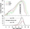 |
Fig. 1 Top: number of MB objects as a function of the absolute magnitude in logarithmic scale. The different colors show different zones of the asteroid belt. Bottom: the two-sample Kolmogorov-Smirnov test; the red curve indicates the middle-inner belt comparison, while the black curve indicates the outer-inner belt comparison (for details, see text). |
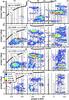 |
Fig. 2 Density distribution of MB objects in the proper (ap, Ip) element space limited to Ip ≤ 20°. Only objects with absolute magnitudes below 15.5 were considered. The eccentricity interval shown on the top of each graph. The density or number (in per cent) of the asteroids inside a cell is shown with different colors (see the legend box); blue corresponds to minimal values (between 2 and 5) and red to maximal values (>20). The size of the cell is |
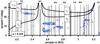 |
Fig. 3 Same as in Fig. 2, except in the very high-eccentricity interval extended to Ip = 35° on the representative (ap, Ip)-plane. |
2.2. The density maps
The qualitative analysis of the distribution of the individual MB objects can be quantified introducing the density index and studying its distribution. The density index is defined as a number of the real objects inside a rectangular cell of dimension  on the (ap, Ip)-plane. The density index is calculated using the objects from our sample and the value obtained is associated with the position of the corresponding cell on the (ap, Ip)-plane. The density presentation is analogous to the averaging process of the real object distribution and depends on the chosen size of the cell. We tested several sizes and found that the one we chose is more appropriate. This cell is neither too small to depict the unnecessary details of the asteroid distribution, nor too large to lose information on its main features.
The density indices obtained are shown in Fig. 2 on the four representative planes corresponding to the different eccentricity intervals and in Fig. 3 corresponding to very high eccentricities. We use red to indicate the regions of the highest density of the objects, which reaches the maximal value of 276 obj/cell in the region of the Veritas family in the outer belt. This value is used to normalize the values of the density index on all eccentricity planes. Blue indicates the regions with the lowest non-zero values, between 2% and 5% of the maximal density, which corresponds to no less than five objects and no more than 13 objects per cell. It is worth observing that, in these regions, less than 13 objects are distributed within the 1.2 × 10⁶ km, equivalent to the size of the cell of 0.008 AU. Despite the fact that such low density of matter is still considered, the absence of the very low-eccentricity objects (with abs. magnitude less than 15.5) in the inner belt is intriguing, as is another anomalously low density region between the 5/2 and 7/3 MMRs with Jupiter, at all eccentricity ranges. Only the low-eccentricity 158 Koronis family (Ip = 2.2° and ep< 0.075) is detected in this region, together with two small, but dense families associated with 293 Brasilia (Ip = 15.0° and ep = 0.12) and 845 Naema (Ip = 12.0° and ep = 0.04). The possible origin of the lack of objects in this region is discussed in Sect. 5.
Figures 2 and 3 show clearly that the distribution of the matter in the MB is highly nonuniform, characterized by agglomerations of the objects around the main asteroidal families and the rarefied background (at least, for adopted limit of the sample). Applying hierarchical clustering method (HCM; Zappalá et al. 1990) and the frequency approach (Carruba & Michtchenko 2009), we have calculated the main families and clusters in the MB; the list is shown in Table F.1. We obtained that the members of the families from this table constitute nearly 30% of the total MB objects from our sample. What draws our attention is that the number of large families, about two dozen (see also Milani et al. 2014, Table 3), is small with respect of the total number of large objects in the MB, which have diameters greater than 100 km, estimated as 189 (see below in Sect. 3.1).
On the density maps, the typical structure of a family consists of a dense and extended along the ap–axis core (red), a mantle (yellow) and a periphery zone (cyan). The main families can be easily identified on the density maps; for instance, in Fig. 2, the largest are the 4 Vesta family in the inner belt, the 15 Eunomia family in the middle belt, and the 221 Eos family in the outer part of the MB; in Fig. 3, the 25 Phocaea and 3 Juno families are clearly seen in the inner and middle belts, respectively. There are also several smaller and compact families, but only the 298 Baptistina family exhibits a different shape, with a large, nearly spherical dispersion of the objects in inclination.
Finally, the atypical boomerang-like structure in the middle belt can be identified on all graphs in Figs. 2 and 3, although its density is lower when compared to the density of the main asteroidal families.
2.3. Frequency distribution of objects in the background of the MB
Analysis of the current distribution of the background objects in proper orbital element space allows us to separate effects of long-lasting diffusion mechanisms produced by the resonances and the Yarkovsky effect on the asteroidal motion from effects of sporadic probabilistic processes. Considering that the asteroids from the AstDyS-catalog (see Figs. B.1 and B.2) are leftover objects of dynamical erosion processes, probabilistic effects can be excluded from the study by eliminating the members of the main asteroidal families from the sample (~30% of total population, Table F.1), which are a product of collisions between asteroids.
The frequency distribution of the MB objects remaining in the background is shown in Fig. 4 in form of the shaded histograms. Solid vertical lines show the current position of the main MMRs with Jupiter. The distribution in proper semimajor axes (top graph) clearly shows three zones delimited by the ν6 SR and the strong Jovial MMRs, which are routes of asteroidal escape from the MB. The populations do not differ significantly between zones. The slight decrease observable in the outer region is attributable to residual bias due to low albedo objects in the zone. The exception is the region between the 5/2 and 7/3 MMRs (2.823 AU–2.956 AU), whose density is only 20% of the density of objects in the middle zone.
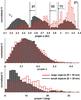 |
Fig. 4 Frequency distribution of MB objects (normalized to total amount) in the proper semimajor axes (top), proper eccentricities (middle), and proper inclinations (bottom). Gray patterns: general background population of the MB (for details, see text). Red patterns: large objects (D> 30 km). Solid vertical lines show the current location of the strong Jovian MMRs. Their location until the sweeping by migrating Jupiter is shown by dashed vertical lines. |
The distribution of the proper eccentricities with mean magnitude at ~0.13 is observed on the middle graph in Fig. 4. This value does not seem to be excessively high, when compared, for instance, to the eccentricity peak of the distribution of the exoplanets1. This is also true for the distribution in inclination (bottom graph in Fig. 4), whose peak lays at 3.̊8 degrees.
To exclude effects of dissipative forces from the study of the dynamical diffusion, we present in Fig. 4 the distribution of the larger objects (red histograms) and compare it to the distribution of the general population (gray histograms). It is expected that the long-lasting Yarkovsky drift is negligible for those asteroids with a diameter larger than 30 km. This limit is somewhat arbitrary and has been chosen with the purpose of comparing our results to those presented in Minton & Malhotra (2009, 2010); this comparison is found in the discussions in Sect. 5.
Comparing the frequencies of the small and large objects of the MB, there is no apparent difference in the eccentricity distribution. The distribution of the large objects in inclination, however, shows the peak of maximum shifted from 3.̊8 to ~10° with respect to the background population. The difference might be due to a bias linked to the fact that most of the surveys dedicated to the discovery of asteroids are designed to search preferentially for objects located around the ecliptic plane. On the other hand, this may also be because excitatio then of inclination by the SRs is more efficient for large objects (see discussion in Sect. 5). Finally, in Fig. 4 it is possible to see a clear increase in the number of large objects as we go from the inner to the outer zones of the MB.
3. Distribution of taxonomies
Considering the evolution of the MB, the most meaningful distinction that can be obtained from taxonomy is whether an object is volatile-poor or volatile-rich, since this classification would indicate that they originally formed closer to or farther away from the Sun than the snow line (Martin & Livio 2013). In this regard, the most fundamental distinction would be between objects of classes belonging to the S-complex (Bus & Binzel 2002) and those classified in the C- or X-complexes (Bus & Binzel 2002), which also have low geometric albedos. The S-complex asteroids, whose spectra is dominated in the visible by olivine/pyroxene bands, in general should have mineralogies compatible with the anhydrous and poorly hydrated chondrites, i.e., OCs and CO/CVs, as well as several products of differentiation (Britt et al. 1992; Burbine & Binzel 2002; Mothe-Diniz et al. 2008). The best mineralogical analogues for objects with low albedo classified in the C-/X-complexes are the hydrated carbonaceous chondrites CM and CI (Vilas & Gaffey 1989; Carvano et al. 2003) Members of these complexes with higher albedos, on the other hand, can be compatible with differentiation products as enstatite achondrites and metallic meteorites, as well as with enstatite chondrites. Also, objects whose spectra show olivine/pyroxene bands with low contrast would also tend to be classified in the C-/X-complexes, as in the case of the Baptistina family (Reddy et al. 2011), but here again the geometric albedo is higher than what is expected for hydrated silicates.
In order to analyze the distribution of the taxonomies of the MB from a dynamical standpoint it is necessary to separate the large objects, whose evolution is determined mostly by planetary perturbations, from the smaller objects, which are also subjected to the Yarkovisky drift. The majority of the larger asteroids have taxonomic classification derived from low-resolution spectroscopy and albedos derived from the IRAS survey, while for the smaller objects the main sources of taxonomic classifications and albedos are the SDSS Moving Object Catalog (Ivezic et al. 2002, 2010) and the WISE/NeoWise (Masiero et al. 2011, 2014) survey. Since all asteroids larger than 50 km have taxonomies derived from spectroscopy, we adopt this limit to define the large asteroid sample. This sample consists of the asteroids with taxonomic classification listed in the SBN database2, with albedos and diameters obtained mostly from IRAS (Tedesco et al. 2004), or in the absence of IRAS data, from the NeoWise survey. For the five asteroids in the sample with no derived albedo, a default value of pv = 0.1 was adopted and the diameter was computed using the classical formula relating absolute magnitude and albedos (Bowell et al. 1989). For the smaller objects, we adopt the taxonomic scheme developed by Carvano et al. (2010) and albedos derived from the NeoWise survey. Here we will use the distribution of the Sp class as a proxy to the volatile-poor asteroids, and the distribution of the Cp/Xp asteroids for the volatile-rich objects (see Appendix C for a discussion on the role of the albedo of the Cp/Xp asteroids).
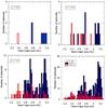 |
Fig. 5 Comparison between the distribution of volatile-poor (red) and volatile-rich (blue) objects with diameters, D, larger than: a) 300 km; b)200 km; c) 100 km; and d) 50 km. |
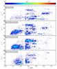 |
Fig. 6 Density maps for Sp asteroids, considering proper eccentricities intervals: a) – ep< 0.075; b) – 0.075 <ep< 0.125; c) – 0.125 <ep< 0.175; and d) – 0.175 <ep< 0.225. |
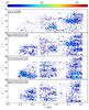 |
Fig. 7 Density maps for Cp/Xp asteroids, considering proper eccentricities intervals: a) – ep< 0.075; b) – 0.075 <ep< 0.125; c) – 0.125 <ep< 0.175; and d) – 0.175 <ep< 0.225. |
3.1. Large objects
Among the three largest asteroids, 1 Ceres, 2 Pallas, and 4 Vesta (Fig. 5a), only 4 Vesta, located at 2.4 AU, has a volatile-poor surface composition resulting from a process of temperature differentiation. The other two asteroids, located at around 2.8 AU, present a surface composition compatible with the presence of abundant volatile material. Taxonomically they have been classified as C and B, respectively, and their albedo of 0.11 and 0.16 is compatible with a carbonaceous rich composition, possibly similar to CM meteorites. Other four asteroids with a diameter larger than 300 km are located beyond 2.8 AU, in the outer region of the MB, all of which present a surface composition compatible with the presence of volatile material and a very low albedo of between 7% and 5%.
Considering all asteroids with an estimated diameter larger than 200 km (Fig. 5b), the number of objects increases to 25, of which 17 have a volatile-rich and eight have a volatile-poor surface composition (68% and 32%, respectively). Three of the volatile-poor objects are located in the inner MB, four in the intermediate, and just one beyond 2.8 AU. The volatile-rich bodies, on the other hand, extend from the intermediate to the outer belt with a higher concentration beyond 3.0 AU, and an albedo smaller than 10%, mostly around 4 − 5%. In the region between 2.8 and 3.05, there is just one large object, (16) Psyche, which is volatile-poor (Kuzmanoski & Kovačević 2002). This asteroid has an estimated diameter of about 250 km and a metallic-rich surface as inferred by diverse measurements (Ostro et al. 1985; Viateau 2000; Matter et al. 2013). According to our current understanding, this object should be the inner core of a differentiated object that was completely disrupted. Moreover, since no dynamical family is associated with this asteroid, the disruption must have occurred in the very early stages of the MB, allowing time for the complete dispersion of the mantle and crust fragments. We can conclude that the volatile-poor objects that are larger than 200 km peak in the inner MB and extend up to 2.9 AU, while the volatile-rich peak beyond 3.0 AU and extend up to nearly 2.4 AU.
The above picture does not significantly change when analyzing the distribution of objects with diameters larger than 100 km (Fig. 5c), although there is a larger spread of volatile-poor objects in the outer part of the MB and of volatile-rich in the inner part. The inner part continues to be dominated by volatile-poor objects, i.e., 16 over 20. On the other hand, in the outer part, beyond 2.8 AU, there are 91 volatile-rich objects against only nine volatile-poor. Globally speaking, 148, or 78% of the asteroids with diameter up to 100 km are volatile-rich, while only 41, or 22%, are volatile-poor.
Finally, if we consider that objects with diameters greater than 50 km and outside strong MMRs are probably at their formation location, then their distribution can be assumed as a picture of the early MB. The heliocentric histogram of these bodies is shown in Fig. 5d. Analyzing their distribution, we find that the volatile-rich and volatile-poor objects are spread around the MB, although the latter represent a smaller fraction. To be more precise, 455, or 78% of the asteroids in this diameter range have a volatile-rich surface composition with low albedo, against only 127 presenting indication of a volatile-poor composition. These results indicate that the MB is mostly composed of volatile-rich bodies (see also DeMeo & Carry 2013) with a minor fraction of volatile-poor objects that are almost uniformly distributed. It is remarkable that in the inner belt, before 2.5 AU, the populations of volatile-poor and volatile-rich large objects almost match in number at 34 and 26, respectively.
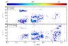 |
Fig. 8 Density maps for asteroids with proper eccentricities ep> 0.225, according to their taxonomy classification. a) Cp/Xp asteroids; b)Sp asteroids. |
3.2. Smaller objects
We use density maps to inspect the distribution of the classes in proper elements. These maps are constructed in the ap × Ip space with bins of 0.024 AU in proper semimajor axis and 20′′ in proper inclination. The bins are color-coded according to the number of asteroids they contain using a logarithmic scale from 1 to 200 objects per bin.
We can now analyze the distribution of the objects of both complexes using the eccentricity ranges defined in the previous sections. These distributions in the first four eccentricity ranges for the Cp and Sp complexes are shown in Figs. 6 and 7, while the distribution for both complexes in the last eccentricity range is shown in Fig. 8. It must be stressed that, although representative of how each population is distributed in the MB, the densities of the Cp/Xp asteroids cannot be directly compared to the distribution of Sp, since no bias correction is performed and the low albedo Cp/Xp asteroids in the SDSS dataset are vastly under-represented due to observational selection effects (DeMeo & Carry 2013).
The Sp objects, for the most part, are present mainly in the vicinity of asteroid families. In particular, in the outer region, Sp are mostly seen in the vicinities of the 221 Eos and 158 Koronis families, with sparser accumulations close to the 5/2 MMR and extending outward from the 7/3 MMR close to the proper inclinations of 158 Koronis family. However, Sp asteroids also seem to cluster in some regions that are not clearly associated with large families. The Sp asteroids fill, with a relatively low density, the inner belt at eccentricities ep< 0.0575 and proper inclinations <7o. Also, more robust accumulations are observed: i) in the region in the middle belt with ep< 0.075 and Ip< 5o, which is clearly cut by the “boomerang-like” gap; see Fig 6a; ii) very distinct accumulations in the “boomerang-like” regions in all other eccentricity intervals; and iii) the broad accumulation in the inner belt centered in the Flora/Baptistina region in the eccentricity range 0.125 <ep< 0.225, which also seems to extend to the adjacent eccentricity ranges. In all of these cases, there are families identified close to the apparent maximum in density, but these families are either too small, oddly shaped, as is the 5 Astraea family inside the “boomerang-like” structure, or both, as is the 298 Baptistina family in the last case. This is the case since 298 Baptistina is only defined robustly as a small family using colors (Parker et al. 2008; Reddy et al. 2011) and the shape of the overdensity in that region seems too broad when compared to even the largest families.
The Cp/Xp asteroids, on the other hand, seem to be present, although sparsely, in the whole MB (Figs. 7 and 8). An exception is the inner MB at ep< 0.075, where they are essentially absent. Besides from the asteroid families, the Cp/Xp asteroids only seem to cluster in the intermediate belt up to 2.7 AU around Ip ≈ 12° and after that semimajor axis value for Ip ≈ 8°.
4. Dynamical portrait of the MB
In this section, we focus on the dynamical mechanisms responsible for the diffusion transport of the objects in the MB. The study is carried out in the form of dynamical and averaged maps, which provide a global dynamical portrait of the MB.
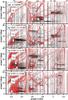 |
Fig. 9 Averaged dynamical maps in the proper elements space limited to Ip< 20°. The red dots are averaged orbital elements of the test particles, whose behavior is affected by MMRs and nonlinear SRs. The black dots are proper elements of the objects from the AstDyS-catalog. The location of the main MMRs is sketched by vertical lines, while the main nonlinear SRs are indicated by the group number from Table A.2. |
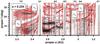 |
Fig. 10 Same as in Fig. 9, except in the very high-eccentricity interval extended to Ip = 35° on the representative (ap, Ip)-plane. |
4.1. Averaged dynamical maps
The construction of the averaged dynamical maps is based on the averaged over 4.2 Myr values of the semimajor axis, eccentricity, and inclination of the asteroidal orbit (Michtchenko et al. 2002); these values are obtained during the construction of the dynamical maps shown in Figs. D.1 and D.2 and are plotted on the representative (ap, Ip)-planes. The averaged maps show the final (after 4.2 Myr of gravitational interactions with the Sun and five planets, from Mars to Neptune) distribution of the test particles, which were initially distributed over a perfectly uniform rectangular grid. The averaged maps allow us i) to detect the slow chaos and ii) to plot the proper elements of real objects over them, since the averaged orbital elements, with good approximation, are the analogue of proper elements. This last property is especially useful if we want to compare the distribution of real objects with respect to the web of resonances in the region under study.
Figures 9 and 10 show the averaged dynamical maps covering all eccentricity intervals that represent the MB. Here we briefly introduce some basic concepts needed to understand the information provided by the maps, while the details may be found in (Michtchenko et al. 2002). In domains free of the MMRs and SRs, small changes in the initial conditions lead to small changes of the proper elements. Consequently, the averaged elements suffer slight displacements on the averaged maps when the initial conditions are gradually changed. In this way, these regions are characterized by the continuous distribution of averaged solutions; in Figs. 9 and 10, these regions appear as regions that do not contain red dots.
On the contrary, in the domains affected by resonances, small changes in the initial parameters can produce large changes of the proper elements. If the chosen time span is long enough, the SAM method is able to detect the sudden displacements and dispersions of the averaged orbital elements. Thus, the domains on the averaged maps associated with the resonances are dominated by the irregular distribution of averaged solutions. These solutions are shown by the red dots in Figs. 9 and 10, where we also plot the nominal location of the main MMRs with vertical lines. The black dots show proper elements of the real objects from the AstDyS–catalog.
In the case of the strong MMRs, such as 3/1, 5/2, 7/3, and 2/1 with Jupiter, the test particles do not even survive during 4.2 Myr leaving the domains of these resonances; on the averaged maps, these resonances appear to be empty. In the case of weaker MMRs, the averaging procedure gathers all resonant particles along the libration centers, whereas the neighborhood of the resonance appears to be empty. The vertical distribution of the red dots matches well with the nominal locations of several weaker MMRs in Figs. 9 and 10.
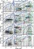 |
Fig. 11 Sketch of the main MMRs (vertical lines) and the strong linear and nonlinear SRs (solid curves) in the MB. The nonlinear SRs are identified by the group number from Table A.2. The dots indicate proper elements of the objects within the corresponding eccentricity interval from the AstDyS catalog. The large objects from the corresponding eccentricity interval are superposed on each graph: red stars indicate objects with diameters D> 100 km, green stars indicate objects with D in the range from 50 km to 100 km, and blue stars indicate objects with 30 km <D< 50 km. |
 |
Fig. 12 Same as in Fig. 11, except in the very high-eccentricity interval extended to Ip = 35° on the representative (ap, Ip)–plane. |
4.2. Averaged dynamical maps and nonlinear secular resonances
In contrast with the vertical distribution of the MMR particles, the distribution of the particles involved in SRs has a complicated structure in the proper (ap, Ip)-subspace. The very strong linear ν6 SR provoking rapid ejection of the objects is responsible for a large gap at the left-hand side of the inner MB; the gap is extended for all eccentricities in Fig. 9. The gap originated by the ν5 SR is located at inclinations higher than 20° and appears only in Fig. 10.
Despite large variations of the orbital elements, the secular resonances known as nonlinear SRs are much weaker and the test particles can remain evolving inside them for a long time. The nonlinear SRs are defined as linear combinations, which obey the resonance condition  where j1,j2,... are simple integers and ∑ i | ji | is the resonance order. According this definition, linear SRs, such as ν5, ν6 and ν16, are of order 1, while nonlinear SRs are of higher order. There are resonances of the g-type involving the perihelia, of the s-type involving nodes and of the gs-type involving both perihelia and nodes of the asteroid and the planets from Mars to Uranus. The resonances generally form bands, due to the peculiar relationships g5 ≅ g7, | g6 | ≅ | s16 | and | g7 | ≅ | s17 |. Table A.2 in Appendix A lists the main bands composed of the nonlinear SRs identified in the MB.
In the inner part of the MB, the most important nonlinear SRs are the low harmonics from band # 1, zk = (kν6 + ν16), k = 2, 3 ..., which affect a large amount of real objects in the inner belt. For instance, as shown in Carruba et al. (2005), some of the V–type asteroids outside the Vesta family are former family members that migrated to their current positions via the interplay of the Yarkovsky effect and nonlinear SRs and MMRs. The harmonics zk form a bundle converging to the linear ν6 resonance. At the low-eccentricity region, the bundle is confined to the close vicinity of the gap formed by the ν6 SR, but, with increasing eccentricities, its width is enlarged and, at ep> 0.15, the bundle encompasses a large portion of the inner belt zone. In addition, there are other important forth-order nonlinear SRs: band # 2 of the gs-type nonlinear SRs and band # 3 of the s-type nonlinear SRs; the complete list of the nonlinear SRs in the inner MB, up to order 5, can be found in Michtchenko et al. (2010). The overlap of these SRs produces a significant degradation of the stability of asteroidal motion in the high- and very high-eccentricity intervals of the inner belt observed in Figs. E.1d and E.2.
At very high eccentricities and inclinations of the inner MB, between the ν6 and ν5 SRs, a considerable amount of the real objects can still be found in AstDyS–catalog (around 1500), despite the fact that the region is visibly affected by strong nonlinear SRs (Fig. E.2). More than 50% of the objects are chaotic with Lyapunov times <25 000; in the case of the 25 Phocaea family, which is unique in the region, the number of chaotic members decreases to 30%. The family is interacting with the nonlinear SRs from bands # 9 – # 11 and many family members are captured inside the strong (ν6 − ν16) nonlinear SR.
The middle MB is densely populated by the strongest low-order nonlinear SRs, in particular, the gs-type z1 = (ν6 + ν16), whose higher harmonics play an important role in the dynamics of the inner belt. The nonlinear SRs form the overlapping bands from # 4 to # 7 listed in Table A.2, whose effects on the distribution of the real objects are noticeable in all eccentricity intervals and at all inclinations (see Fig. B.1). Probably, the most curious feature is the boomerang-like structure, which can be clearly associated with the action of the resonances from band # 5, the g-type (2 ν6 − ν5) and (2 ν6 − ν7) nonlinear SRs, especially on graphs c and d and Fig. B.2. The location and shape of the SRs change significantly for different values of proper eccentricity. This explains the transformation of the boomerang-like feature from the void of the real objects, at small eccentricities (panels a and b in Fig. B.1), to the dense agglomeration, at moderate and high eccentricities (panels c and d in Fig. B.1).
The boomerang-like agglomeration is also present at the very high-eccentricity interval of the middle belt shown in Fig. and B.2. The 3 Juno and the 410 Chloris families are accommodated in the low-inclination domains free of the important nonlinear SRs. On the contrary, the high-inclined 945 Barcelona family, at  , is located at intersection of two strong nonlinear SRs, ν6 − ν16 and ν6 − ν14, from bands # 11 and # 12, respectively, and the majority of its members are evolving in of one of these resonances. The 2 Pallas group is confined between two components of the band # 12.
Finally, in the outer zone of the MB, the nonlinear SRs lose strength and their widths decrease; this occurs because the linear SR, ν5, ν6, and ν16, whose linear combinations give origin to the nonlinear SRs, are far away from the main bulk of objects in the outer belt. Figure 9 shows several bands, such as # 4, # 5, # 7, and # 8 (Table A.2), present in this region, however their overlap is not observed. Despite the decreasing strength of the SRs in the outer zone, there are several records of their interaction with the asteroidal families in the region, for instance, with the 158 Koronis family (Tsiganis et al. 2003) and the 221 Eos family (Vokrouhlický et al. 2006). In the very high-eccentricity region, there is only the 31 Euphrosyne family, at  , which is located very close to the linear ν6 SR and several of its members are interacting with this resonance (see Fig. 10).
5. Discussion on possible constraints
In this section, the spatial and compositional distributions of MB objects shown in the previous sections are analyzed, searching for possible constraints on the physical processes that could be responsible for some features of the MB, such as its excitation, depletion, and radial mixing of two distinct populations: volatile-poor and volatile-rich populations (O’Brien & Sykes 2011). The analysis is supported by several numerical simulations of the long-term asteroidal evolution upon action of gravitational perturbations by the planets, from Mars to Neptune, and nongravitational thermal Yarkovsky effects.
5.1. Dynamical excitation
One of the features of the MB frequently mentioned in the literature is a dynamical excitation of its objects (e.g., Petit et al. 2001; O’Brien et al. 2007). Indeed, the current theories of planet formation assume that, initially, the eccentricities and inclinations of the primordial MB objects were low enough for the accretion processes to occur. The current distributions of these orbital parameters, however, exhibit the peaks at ~0.13 and  , respectively (see Fig. 4). These values, although considered to be evidence for the “strong excitation” some years ago, presently may not be considered excessively high, if compared, for instance, to the eccentricity peak of the distribution of the exoplanets, which lies between 0.1 and 0.4. We can suppose that the mechanisms responsible for the dynamical excitation in the solar system were weaker than those invoked in scenarios involving substantial planetary migrations. The absence of “hot Jupiter” in the solar system could support this hypothesis.
In the present work, we have found evidence in the distribution of the background MB objects that MMRs and SRs (see Sect. 4), overlaying with the slow dissipative Yarkovsky drift, may contribute substantially to the enhancement of the proper eccentricities and inclinations in the MB. To show this, we plot in Fig. 13 the distribution in proper eccentricities (top panel) and inclinations (bottom panel) of the background objects (as defined in section 2.3) separated between the inner (gray), middle (red), and outer (black) zones of the MB. We observe that the populations of the inner and outer zones are distinctly distributed. The inner MB objects tend to agglomerate at higher eccentricities with the peak at 0.15, and at lower inclinations with the peak at 3.̊5. On the contrary, the outer MB objects are more uniformly distributed with the eccentricity peak at ~0.1 and the inclination peak at 11°.
The difference can be explained by the fact that the dynamical mechanisms acting on the drifting objects in the inner and outer zones are distinct. As described in Sect. 4, the dynamics in the inner MB is dominated by the SRs, in particular, by the very strong ν6 SR and its harmonics, whose action enhances the asteroid eccentricities (see Figs. E.1–E.2). The very low density of objects and the absence of families at eccentricities below 0.075 shown in Fig. 2 are a possible consequence of this process. In contrast, the outer MB is dominated by the strong two- and three-body MMRs, affecting both the eccentricities and inclinations of the objects. These orbital elements can be either enhanced or decreased, depending on the direction of the crossing MMR object, and their distribution in the outer MB is more homogenous (see Fig. 13). Finally, as expected, the distributions of the middle MB objects accounts for both mechanisms of excitation.
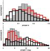 |
Fig. 13 Comparative distribution of the background objects in the inner MB (gray patterns), middle MB (red line), and outer MB (black line). Top: in the proper eccentricities. Bottom: in the proper inclinations. |
It must also be mentioned that other mechanisms, some of which not yet well understood, could also produce the observed excitation of the MB. One example is the recent work by Veras et al. (2015), which models the orbital evolution of asteroids under the effect of stellar radiation and winds. In particular, the authors study the long-lasting Yarkovsky effects on the eccentricity and inclination evolution of the small bodies. They demonstrate that the Yarkovsky effect can alone dominate the eccentricity and inclination evolution of bodies citing the Eos family as an example.
Hence, there seem to be strong grounds to believe that the combination of those mechanisms working over the ≈4 Gyr since the gas in the disk was dissipated and the planets acquired their present configuration could substantially modify the distributions of eccentricities and inclinations in the MB. This is something that must not be overlooked when trying to compare the result of migration/accretion models to the present day MB. Petit et al. (2001), for example, claim that this characteristics of the MB is a byproduct of a dynamical removal mechanism associated with the late stages of planet formation. Their model shows that Jupiter’s formation could have produced sweeping resonances and/or the scattering and excitation of large planetary embryos within the MB, thereby eliminating most of the bodies from the primordial MB shortly after Jupiter reached full size (i.e., presumably some 10 Myr. after the formation of planetesimals). Other models whose end result match the dynamical excitation seen in the present-day MB is the Grand Tack scenario (Walsh et al. 2012), which assumes that during the gas phase the proto-Jupiter would have migrated inward down to 1.5 AU and then back to 5.5 AU. Conversely, the model of Izidoro et al. (2015), which assumes several ad hoc mass density profiles during the accretion in the MB, was considered unsuccessful by the authors because in all their results the MB was less excited than what is presently observed. In all those cases, the authors failed to consider the posterior evolution of eccentricities and inclinations in the MB and, therefore, their conclusions must be seen with some reserve.
5.2. Mass depletion
It was first proposed that most of the primordial mass of the MB was removed by collisional erosion (e.g., Chapman & Davis 1975). However, as discussed in O’Brien & Sykes (2011), there is numerous evidence against this suggestion; meanwhile, a number of other mechanisms invoked to deplete the mass of the MB during the early stages of the solar system, because of a limited amount of observational data, are yet to be confirmed.
In this work we argue in favor of the long-lasting dynamical diffusion transport and a consequent loss of MB objects. This depletion scenario can be schematically decomposed into two components: One is a “horizontal” diffusion of objects inward/outward to the Sun, which is caused by dissipative forces, such as the Yarkovsky/Yorp effects, that essentially affect the semimajor axis of an object. The other component is a “vertical” diffusion, which affects the objects captured in the weak MMRs and nonlinear SRs described in Sect. 4.
The most important MMRs and SRs are sketched in Figs. 11 and 12. It is easy to distinguish the MMRs from Table A.1, which appear as vertical lines, from the SRs indicated by the corresponding group number from Table A.2. (The meaning of the words “horizontal” and “vertical” is now evident from a simple look at Fig. 11). Both processes are size-dependent: Larger bodies, whose response to the Yarkovsky effect is weak, perform long-lasting drifts along the weak MMRs and nonlinear SRs (Carruba et al. 2005), while the smaller bodies are more susceptible to the Yarkovsky effects and their diffusion is directed mainly inward/outward with respect to the Sun. Both components are very slow, lasting over billions of years until the objects reach regions of strong instabilities, which are responsible for ejection of the bodies from the MB (e.g., Migliorini et al. 1998). These regions are associated with i) low-order MMRs with Jupiter, such as 3/1, 5/2, 7/3, and 2/1; and ii) linear SR, such as ν5, ν6 and ν16. The ejection of the bodies from the MB is very rapid in these regions with characteristic times shorter than a few million years.
The slow diffusion processes cannot be observed directly, but their records can be found in the current distribution of MB objects described in previous sections. One of these is a very low density of the background objects in the region between the 5/2 and 7/3 MMRs with Jupiter, clearly observed on the density maps in Figs. 2 and 3, at all values of the asteroidal eccentricity, where there are essentially only three asteroidal families: 158 Koronis, 293 Brasilia, and 845 Naema. The region is confined between two gaps corresponding to the 5/2 and 7/3 Jovial MMRs and its narrow width makes the depletion very efficient; this is further due to the presence of the band formed by the important MMRs, the 6/1 MMR with Saturn, and two three-body MMR, 7J:-5S:-2A and 2J:1S:-1A, in the middle of the region. An evidence that the diffusion transport of objects is still ongoing is the streak of S-type objects from 158 Koronis that cross the 7/3 MMR into the outer part of the MB (see Sect. 3.2 and Fig. 6).
To confirm this hypothesis, we performed a numerical simulation of the long-term evolution of test particles upon perturbations of five planets, from Mars to Neptune, accounting for Yarkovsky effects. To simulate the Yarkovsky effects, we use SWIFT-RMVSY, the version of SWIFT modified by Brož (1999), to account for both the diurnal and seasonal versions of the Yarkovsky effect. We fix the set of the physical and thermal parameters as follows: R = 1000 m, ρbulk = 3500 kg/m3, ρsurf = 1500 kg/m3, K = 2.65 W/m3/K, C = 680 J/Kg/K, A = 0.09, and ϵ = 0.9, where R, ρbulk, ρsurf, K, C, A, and ϵ are the radius, bulk density, surface density, thermal conductivity, thermal capacity, albedo, and infrared emissivity of the objects, respectively. The period of rotation is assumed be proportional to the inverse of the radius as in Farinella et al. (1998). The simulated asteroids have constant obliquity; they are either prograde rotators with 0-obliquity, or retrograde rotators with 180°–obliquity. In the former case, the diurnal Yarkovsky effect is antidissipative, and the semimajor axis evolves toward larger values, whereas, in the latter case, the evolution occurs toward smaller a. We do not consider reorientations of spin axis via collisions or YORP (Čapek & Vokrouhlický 2004). It is important to stress that these assumptions lead to nonrealistic results for the timescale of the dynamical evolution of asteroids, but still allow us to perform a qualitative study of the asteroidal evolution upon the dissipative forces.
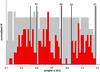 |
Fig. 14 Frequency distribution of the initially uniformly distributed along the semimajor axis objects with the radius of 1000 m, after 2 × 10⁵ yr (gray) and 1.2 × 10⁹ yr (red) of the evolution under perturbations of the five planets and Yarkovsky effects. |
Thus, 480 identical particles (except one half of them were 0-rotators and other half was 180°-rotators) were uniformly distributed across the semimajor axis, from 2.1 AU up to 3.3 AU, with spacing of 0.005 AU. The initial values of the eccentricities and inclinations were fixed at 0.13 and 5°, respectively, which correspond approximately to the peaks in the distributions of the orbital elements in Fig. 4; the angular elements were arbitrary. The thermal parameters of the particles were chosen from the set described above and all particles had a radius of 1000 m. Figure 14 shows the distribution of these particles at two instants of their evolution: after 200 000 years (gray color) and 1.2 Gyrs (red color). The lack of objects between the 5/2 and 7/3 MMRs can be clearly observed at the instant following the very long-lasting evolution of the MB, and also at locations of the ν6 and ν16 SRs and 3/1 and 2/1 MMRs.
It is worth emphasizing that the simulation of the dynamical erosion of the MB large objects (i.e., without dissipative Yarkovsky drift) during the 4 Gyr dynamical evolution performed in Minton & Malhotra (2010) did not detect the depletion in this region (see Fig. 4 in that paper). This fact is supported by observational distribution of large bodies shown with a red solid line in the top of Fig. 4. On the other hand, the shaded histogram presenting the distribution of the small objects in the same figure clearly shows an accentuated depletion between the 5/2 and 7/3 MMRs. The distinct distributions of the large and small bodies indicate that the mechanisms of depletion acting in this region are size dependent. Thus, the Yarkovsky drift seems to be adequate process, in contrast with the size-independent sweeping MMRs due to migrating Jupiter suggested in Minton & Malhotra (2009).
The other evidence for the efficient diffusion transport in the MB are the dynamically produced accumulations of objects detected in our analysis. For instance, the two most distinctive features are the boomerang-like structure and the overdensity of objects around the 298 Baptistina family.
The boomerang-like structure in the middle region is an unequivocal evidence for the diffusion transport mechanisms acting in the MB. Figure 11 shows that it is associated with band # 5 formed of two strong g-type nonlinear SRs, (2 ν6 − ν5) and (2 ν6 − ν7). At small eccentricities (<0.1), the band originates a void of asteroids (see Fig. B.1), which can be explained by the fact that the g-type resonances strongly excite the asteroidal eccentricities. In fact, at moderate and high eccentricities, the agglomeration of the objects along the whole extension of band # 5 is observed; this band contains ~20 000 asteroids from the AstDyS archive. An interesting fact here, however, is that this structure seems to be composed mostly of volatile-poor, or Sp-type, asteroids (see Figs. 6 and 7). This could be a bias effect, since the higher albedo volatile-poor objects are sampled in the SDSS data to much smaller diameters than the dark volatile-rich objects. Another possibility for the predominance of volatile-poor asteroids is the breakup of a volatile-poor parent body inside the boomerang region. In fact, an S-type family, 5 Astraea, is identified in this region by Milani et al. (2014). However, the family is oddly shaped, and the fact that the dynamics of the region by itself seems able to produce an accumulation of objects in this regions casts some doubts on whether Astrea is a real collisional family.
The 298 Baptistina group is located in the dynamically active region of the inner MB, where the weak MMRs intersect bands # 1 – # 3 of the SRs (Fig. 11c). The superposition of many, even weak, resonances may produce efficient mechanisms to disperse the population in the region of overlapping. There are several signs that the objects from the Baptistina region have experienced the effects of these mechanisms. These are: i) the enhancement of the background density (see Figs. 2b,c); ii) the elevated concentration of large asteroids, with D> 10 km (see Fig. 11 in Michtchenko et al. 2010); iii) the increased percentage of objects in chaotic orbits (see Fig. E.1); and finally iv) the considerable dispersion in inclination and irregular shape of the 298 Baptistina group, contrasting with the shapes of the other families (see Fig. B.1). A detailed study of this group has been addressed in Reddy et al. (2011).
5.3. Radial mixing
The classical planet formation theories predict that a primordial temperature gradient existed during the accretionary phase and would produce a compositional gradient across the asteroid belt, from higher-temperature refractory materials in the inner zone to lower-temperature carbonaceous materials and water ice in the outer zone. The peculiar position of the snow line, just in the middle of the MB at 2.7 AU (Martin & Livio 2013), would be the most obvious reason for the distinct compositions. However, as noted since the first surveys of compositions in the MB (e.g., Gradie & Tedesco 1982), the observational data show significant overlap and our analysis in Sect. 3 confirms this fact. This has been interpreted as suggestive of radial mixing of bodies in the MB subsequent to their formation.
However, most recent works on disk evolution invoke diverse mechanisms for the transport and mixing of compositions (e.g., Ciesla 2010; Ciesla & Sandford 2012; Jacquet & Robert 2013; Ali-Dib et al. 2015) in the early stages and these could be, at least in part, responsible for the radial mixing presently observed in the MB. In this sense, the observed mixing of compositions could have occurred before the end of the planet formation. This would solve the problem of features that are not easily explained through “cold” dynamical processes. The most clear example is the orbital distribution of large asteroids with D> 50 km. Volatile-rich objects are more frequent in the outer belt, but present on all MB (Figs. 14 and 7, see also DeMeo & Carry 2013); the same picture holds whether considering small or large objects. On the other hand, the distribution of the volatile-poor objects seems different whether one considers large or small asteroids. The number of large volatile-poor objects varies only slightly between the inner, middle and outer zones (34, 51, and 42, respectively), suggesting an almost uniform distribution (Fig. 5d, see also Mothé-Diniz et al. 2003). However, the small Sp-type asteroids in the outer belt are sparse and either concentrated around the 221 Eos and 1400 Tirela families or in the streak that seems to originate on the 158 Koronis family. At this point, the reason for this discrepancy is not clear.
To explain the overabundance of the volatile-rich material in the inner MB, we can also analyze the properties of the MMRs and Yarkovsky drift. It is known that the effect of MMRs (such as 3/1, 5/2 and 7/3 MMRs) on orbits of migrating objects is not symmetric with respect to the direction of the horizontal drift. If particles cross a MMR from left to right, the probability of their capture inside the MMR is high. As a consequence, the particles generally evolve inside the MMR, to be ejected from the MB. Only a very small portion is likely to cross the resonance drifting in the direction of increasing a (e.g., Folonier et al. 2014). On the contrary, the probability of the particle drifting in the opposite direction to cross the resonance and continue drifting is considerable. In addition, the Yarkovisky rate is inversely proportional to the albedo and to the bulk density of an object (Brož 1999). Since the volatile-rich classes tend to have both lower albedos and bulk densities (DeMeo & Carry 2013), they are more efficient MMR crossers in the direction of smaller semimajor axes than the volatile-poor objects drifting toward larger a. In this way, the described mechanism may be responsible, at least partially, for the radial mixing of background objects.
6. Conclusions
In the previous sections, we have outlined the principal characteristic of the MB in terms of mass distribution and segregation of the two main compositional classes. We also have highlighted the most important dynamical processes that have been operating on this population since the planets achieved their current orbits. From what has been presented, it is then possible to understand several features of the distribution of the objects in the MB today as a product of the continuous evolution in this dynamically “cold” stage. In particular, these processes can explain the depletion of objects in some regions as well as their accumulation in others (excluding the families as a product of collisional activity).
The working hypothesis tested in this paper is that the current spatial and compositional configuration of MB objects could be produced by their long-lasting evolution in the so-called “cold” stage of 4.5 Gyr duration, upon gravitational perturbations of the already formed solar system planets and thermal torques. We have detected several records in the MB distributions that support our hypothesis and have reconstructed some of the detected features through numerical simulations. The suggested scenario is able to explain several aspects of the MB. It should be stressed, however, that the conclusions obtained do not invalidate other scenarios proposed in the literature, but caution and critical view are necessary when introducing “catastrophic” models.
In summary, we have described the most relevant distributions of the material in the MB which provide important constraints for modeling the origin and evolution of the MB. We have also shown that many of the current features can be explained by the interplay of diverse dynamical mechanisms because of the planetary perturbations over 4 Gyr with nongravitational effects (e.g., Yarkovsky/Yorp drift). Nevertheless, dynamical evolution alone seems unable to explain some of the observed properties, such as the orbital distribution of volatile-poor and volatile-rich asteroids. The origin of these objects is most probably associated with the earlier stages of the solar system, during the accretion phase of the planetesimals and of the Sun itself. Further observational data will allow us to better understand the mixing processes of material and the structure of the early solar system in the presence of shifted snow line (Martin & Livio 2013). For the present, our limited understanding of disk structure, formation, and early evolution of planetary systems makes it difficult to obtain solid conclusions about this phase of the MB evolution. The present day distributions are the only witnesses we have that can be imposed on the current models of solar system evolution. The present work provides a contribution in this direction.
For details, see histogram plots on http://exoplanets.org
Acknowledgments
This work was supported by the Brazilian National Research Council, CNPq, through diverse research fellowships. D.L. and J.M.C. have also been supported by the Brazilian agency FAPERJ (grant E-26/102.967/2011) and TAM by FAPESP (grant 2014/13407-4). This work has made use of the facilities of the Computation Center of the University of São Paulo (LCCA-USP) and of the Laboratory of Astroinformatics (IAG/USP, NAT/Unicsul), whose purchase was made possible by the Brazilian agency FAPESP (grant 2009/54006-4) and the INCT-A.
References
- Ali-Dib, M., Martin, R. G., Petit, J.-M., et al. 2015, A&A, 583, A58 [NASA ADS] [CrossRef] [EDP Sciences] [Google Scholar]
- Alvarez-Candal, A., Duffard, R., Lazzaro, D., & Michtchenko, T. 2006, A&A, 459, 969 [NASA ADS] [CrossRef] [EDP Sciences] [Google Scholar]
- Bowell, E., Hapke, B., Domingue, D., et al. 1989, In Asteroids II, eds. R. P. Binzel, T. Gehrels, & M. S. Matthews (Tucson: The University of Arizona Press), 524 [Google Scholar]
- Britt, D. T., Tholen, D. J., Bell, J. F., & Pieters, C. M. 1992, Icarus, 99, 153 [NASA ADS] [CrossRef] [Google Scholar]
- Brož, M. 1999, Diploma thesis, Charles Univ. [Google Scholar]
- Burbine, T. H., & Binzel, R. P. 2002, Icarus, 159, 468 [NASA ADS] [CrossRef] [Google Scholar]
- Bus, S. J., & Binzel, R. P. 2002, Icarus, 158, 146 [NASA ADS] [CrossRef] [Google Scholar]
- Čapek, D., & Vokrouhlický, D. 2004, Icarus, 172, 526 [NASA ADS] [CrossRef] [Google Scholar]
- Carruba, V., & Michtchenko, T. A. 2009, A&A, 493, 267 [NASA ADS] [CrossRef] [EDP Sciences] [Google Scholar]
- Carruba, V., Michtchenko, T. A., Roig, F., Ferraz-Mello, S., & Nesvorný, D. 2005, A&A, 441, 819 [NASA ADS] [CrossRef] [EDP Sciences] [Google Scholar]
- Carruba, V., Roig, F., Michtchenko, T. A., Ferraz-Mello, S., & Nesvorný, D. 2007, A&A, 465, 315 [NASA ADS] [CrossRef] [EDP Sciences] [Google Scholar]
- Chapman, C. R., & Davis, D. R. 1975, Science, 190, 553 [NASA ADS] [CrossRef] [Google Scholar]
- Carvano, J. M., Mothé-Diniz, T., & Lazzaro, D. 2003, Icarus, 161, 356 [NASA ADS] [CrossRef] [Google Scholar]
- Carvano, J. M., Hasselmann, P. H., Lazzaro, D., & Mothé-Diniz, T. 2010, A&A, 510, A43 [NASA ADS] [CrossRef] [EDP Sciences] [Google Scholar]
- Ciesla, F. J. 2010, ApJ, 740, 1 [Google Scholar]
- Ciesla, F. J., & Sandford, S. A. 2012, Science, 336, 452 [NASA ADS] [CrossRef] [Google Scholar]
- DeMeo, F. E., & Carry, B. 2013, Icarus, 226, 723 [NASA ADS] [CrossRef] [Google Scholar]
- Gomes, R., Levinson, H. F., Tsiganis, K., & Morbidelli, A. 2005, Nature, 435, 466 [NASA ADS] [CrossRef] [PubMed] [Google Scholar]
- Farinella, P., & Vokrouhlický, D. 1999, Science, 283, 1507 [NASA ADS] [CrossRef] [PubMed] [Google Scholar]
- Farinella, P., Vokrouhlický, D., & Hartmann, W. K. 1998, Icarus, 132, 378 [NASA ADS] [CrossRef] [Google Scholar]
- Folonier, H. A., Roig, F., & Beaugé, C. 2014, Celest. Mech. Dyn. Astron., 119, 1 [NASA ADS] [CrossRef] [Google Scholar]
- Froeschlé, Ch., & Scholl, H. 1989, Celest. Mech. Dyn. Astron., 46, 231 [NASA ADS] [CrossRef] [Google Scholar]
- Gallardo, T. 2014, Icarus, 231, 273 [NASA ADS] [CrossRef] [Google Scholar]
- Gradie, J., & Tedesco, E. 1982, Science, 216, 1405 [NASA ADS] [CrossRef] [PubMed] [Google Scholar]
- Ivezic, Z., Juric, M., Lupton, R. H., Tabachnik, S., & Quinn, T. 2002, SPIE Conf. Ser., 4836, 98 [NASA ADS] [Google Scholar]
- Ivezic, Z., Juric, M., Lupton, R. H., et al. 2010, Nasa Planetary System, 124 [Google Scholar]
- Izidoro, A., Raymond, S. N., Morbidelli, A., & Winter, O. C. 2015, MNRAS, 453, 3619 [NASA ADS] [CrossRef] [Google Scholar]
- Jacquet, E., & Robert, F. 2013, Icarus, 223, 722 [NASA ADS] [CrossRef] [Google Scholar]
- Knežević, Z., & Milani, A. 1994, in Asteroids, Comets, Meteors 1993, eds. A. Milani, M. Di Martino, & A. Cellino (Dordrecht: Kluwer Acad. Publ.), 143 [Google Scholar]
- Knežević, Z., & Milani, A. 2000, Celest. Mech. Dyn. Astron., 78, 17 [NASA ADS] [CrossRef] [Google Scholar]
- Knežević, Z., & Milani, A. 2003, A&A, 403, 1165 [NASA ADS] [CrossRef] [EDP Sciences] [Google Scholar]
- Krasinsky, G. A., Pitjeva, E. V., Vasilyev, M. V., & Yagudina, E. I. 2002, Icarus, 158, 98 [CrossRef] [Google Scholar]
- Kuchynka, P., & Folkner, W. M. 2013, Icarus, 222, 243 [NASA ADS] [CrossRef] [Google Scholar]
- Kuzmanoski, M., & Kovačević, A. 2002, A&A, 395, L17 [NASA ADS] [CrossRef] [EDP Sciences] [Google Scholar]
- Martin, R. G., & Livio, M. 2013, MNRAS, 428, L11 [NASA ADS] [Google Scholar]
- Masiero, J. R., Mainzer, A. K., Grav, T., et al. 2011, ApJ, 741, 68 [NASA ADS] [CrossRef] [Google Scholar]
- Masiero, J. R., Grav, T., Mainzer, A. K., et al. 2014, ApJ, 791, 121 [NASA ADS] [CrossRef] [Google Scholar]
- Matter, A., Delbo, M., Carry, B., & Ligori, S. 2013, Icarus, 226, 419 [NASA ADS] [CrossRef] [Google Scholar]
- Michtchenko, T. A., Lazzaro, D., Ferraz-Mello, S., & Roig, F. 2002, Icarus, 158, 343 [NASA ADS] [CrossRef] [Google Scholar]
- Michtchenko, T. A., Lazzaro, D., Carvano, J. M., & Ferraz-Mello, S. 2010, MNRAS, 401, 2499 [NASA ADS] [CrossRef] [Google Scholar]
- Migliorini, F., Michel, P., Morbidelli, A., Nesvorny, D., & Zappala, V. 1998, Science, 281, 2022 [NASA ADS] [CrossRef] [Google Scholar]
- Milani, A., & Knežević, Z. 1990, Celest. Mech. Dyn. Astron., 49, 347 [NASA ADS] [CrossRef] [Google Scholar]
- Milani, A., & Knežević, Z. 1992, Icarus, 98, 211 [NASA ADS] [CrossRef] [Google Scholar]
- Milani, A., & Knežević, Z. 1994, Icarus, 107, 219 [NASA ADS] [CrossRef] [Google Scholar]
- Milani, A., Cellino, A., Knežević, Z., et al. 2014, Icarus, 239, 46 [NASA ADS] [CrossRef] [Google Scholar]
- Minton, D. A., & Malhotra, R. 2009, Nature, 457, 1109 [NASA ADS] [CrossRef] [PubMed] [Google Scholar]
- Minton, D. A., & Malhotra, R. 2010, Icarus, 207, 744 [NASA ADS] [CrossRef] [Google Scholar]
- Morbidelli, A., Brasser, R., Gomes, R., Levinson, H. F., & Tsiganis, K. 2010, AJ, 140, 1391 [NASA ADS] [CrossRef] [Google Scholar]
- Mothé-Diniz, T., Carvano, J. M., & Lazzaro, D. 2003, Icarus, 162, 10 [NASA ADS] [CrossRef] [Google Scholar]
- Mothé-Diniz, T., Carvano, J. M., Bus, S. J., Duffard, R., & Burbine, T. H. 2008, Icarus, 195, 277 [NASA ADS] [CrossRef] [Google Scholar]
- O’Brien, D. P., & Sykes, M. V. 2011, Space Sci. Rev., 163, 41 [NASA ADS] [CrossRef] [Google Scholar]
- O’Brien, D. P., Morbidelli, A., & Bottke, W. F. 2007, Icarus, 191, 434 [NASA ADS] [CrossRef] [MathSciNet] [Google Scholar]
- Ostro, S. J., Campbell, D. B., & Shapiro, I. I. 1985, Science, 229, 442 [NASA ADS] [CrossRef] [Google Scholar]
- Parker, A., Ivezic, Z., Juric, M., et al. 2008, Icarus, 198, 138 [NASA ADS] [CrossRef] [Google Scholar]
- Petit, J.-M., Morbidelli, A., & Chambers, J. 2001, Icarus, 153, 338 [NASA ADS] [CrossRef] [Google Scholar]
- Reddy, V., Carvano, J. M., Lazzaro, D., et al. 2011, Icarus, 216, 184 [NASA ADS] [CrossRef] [Google Scholar]
- Rubincam, D. P. 2000, Icarus, 148, 2 [NASA ADS] [CrossRef] [Google Scholar]
- Strom, R. G., Malhotra, R., Ito, T., Yoshida, F., & Kring, D. A. 2005, Science, 309, 1847 [NASA ADS] [CrossRef] [PubMed] [Google Scholar]
- Tedesco, E. F., Noah, P. V., Noah, M., & Price, D. D. 2004, IRAS Minor Planet Survey. IRAS-A-FPA-3-RDR-IMPS-V6.0. NASA Planetary Data System [Google Scholar]
- Tsiganis, K., Varvoglis, H., & Morbidelli, A. 2003, Icarus, 166, 131 [NASA ADS] [CrossRef] [Google Scholar]
- Veras, D., Eggl, S., & Gänsicke, B. T. 2015, MNRAS, 451, 2814 [NASA ADS] [CrossRef] [Google Scholar]
- Viateau, B. 2000, A&A, 354, 725 [NASA ADS] [Google Scholar]
- Vilas, F., & Gaffey, M. J. 1989, Science, 246, 790 [NASA ADS] [CrossRef] [PubMed] [Google Scholar]
- Vokrouhlický, D., Brož, M., Morbidelli, A., et al. 2006, Icarus, 182, 92 [NASA ADS] [CrossRef] [Google Scholar]
- Walsh, K., Morbidelli, A., Raymond, S. N., O’Brian, D. P., & Mandell, A. M. 2012, MAPS, 47, 1941 [Google Scholar]
- Weidenschilling, S. J. 1977, Astrophys. Space Sci., 51, 153 [NASA ADS] [CrossRef] [Google Scholar]
- Williams, J. G., & Faulkner, J. 1981, Icarus, 46, 390 [NASA ADS] [CrossRef] [Google Scholar]
- Zappalá, V., Cellino, A., Farinella, P., & Knezevic, Z. 1990, AJ, 100, 2030 [NASA ADS] [CrossRef] [Google Scholar]
Appendix
The main nonlinear SRs present in the region of the asteroidal belt, below ν6. The linear resonances (of first order) are of (i) the g-type with a generic argument νi = g − gi, which are formed by the combination of the proper frequency of perihelion g and the fundamental frequencies of the precession of the planet perihelia, from Mars (i = 4) to Uranus (i = 7); (ii) the s-type with a generic argument ν1i = s − si, where s and si are the proper frequency of node s and the fundamental frequencies of the planet nodes precession, si.
The main MMRs present in the asteroidal belt.
Main nonlinear SRs, present in the region of the asteroidal belt below the ν6 SR.
Appendix B: The representative planes
To show the distribution of the asteroids in the three-dimensional proper elements space (ap, ep, Ip), we follow the approach used by Milani & Knežević (1992): the sample of the objects is separated in different eccentricity intervals and each one is presented on the (ap, Ip)-plane of the proper semimajor axis and inclination. Hereafter we refer to this plane as “the representative plane”. We prefer to display the (ap, Ip)-plane, instead of the widely used (ap, ep)-plane, because the dispersion of the asteroidal families in inclination is significantly smaller than in eccentricity and semimajor axis. As a consequence, the families appear confined to the narrow horizontal regions on the (ap, Ip)-plane. (This feature can be easily understood in the context of the orbital dynamics; to change the plane of its orbits, a particle must gain several orders more kinetic energy than the energy necessary to change its semimajor axis and eccentricity.)
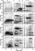 |
Fig. B.1 An overview of the MB objects on the four representative (ap, Ip)-planes. |
We have arbitrarily chosen five eccentricity intervals. The first interval is characterized by very low eccentricities, less than 0.075. The second interval covers low-to-moderate eccentricities within the range 0.075 ≤ ep< 0.125. The next two intervals cover the moderate (0.125 ≤ ep< 0.175) and high (0.175 ≤ ep< 0.225) eccentricities, respectively. Finally, the very high-eccentricity region is defined by ep ≥ 0.225. Because of the peculiarities of the distribution of highly eccentric orbits, this last interval is shown separately, while the others are always presented together with the purpose of their comparison.
Figure B.1 gives an overview of the distribution of MB objects on the representative planes. The main asteroidal families can be easily identified as the dense, horizontally extended agglomerations of the objects. However, there are also some different structures whose shapes clearly contrast with those of the asteroidal families. One of these appears in the inner belt at eccentricities above 0.075, where we can observe a vertically-dispersed agglomeration of the objects; this agglomeration is sometimes referred to as “the Baptistina family” (former region of the Flora family). The properties and origin of this agglomeration has been already discussed in Michtchenko et al. (2010) and in Reddy et al. (2011).
In the middle belt, we also identify an unusual boomerang-like structure, which evolves from the gap, at very low eccentricities (graph a in Fig. B.1), to the agglomeration of the objects, at high eccentricities. Later we will show that this structure is associated with the overlap of several strong nonlinear SRs in this region. The apparent dearth of background objects in the passage from the middle to the outer zones, between the 5/2 and 7/3 MMRs with Jupiter, is shown in Fig. B.1, which is more pronounced in domains of eccentricities above 0.1, on graphs c and d, which are free from large asteroidal families.
Finally, the very high-eccentricity objects, with ep> 0.225, are shown in Fig. B.2; in this case, the upper limit is extended to Ip = 35° on the graph. The boomerang-like agglomeration still exists in this region, along with a few asteroidal families: in the inner belt, the 25 Phocaea family at  ; in the middle belt, the 3 Juno family at
  , the 410 Chloris family at
  and the very high-inclined dense 945 Barcelona family at ; and, in the outer belt, the small and dense 778 Theobalda family at
  , and the high-inclined 31 Euphrosyne family at
  .
.
Appendix C: Distribution of asteroids according to their classification
Figure C.1a–c compares the distribution of all asteroids classified as Cp/Xp with two subsamples of that population: one with WISE albedo pV< 0.1 and the other with pV> 0.1. It is clear here that the low albedo asteroids dominate the Cp/Xp population and that its distribution closely matches the distribution of all Cp/Xp asteroids, while the high albedo Cp/Xp asteroids only dominate around the 298 Baptistina and 221 Eos families (and also slightly above the Vesta family). Keeping that in mind, we consider at this stage that the distribution of all Cp/Xp asteroids is representative of the distribution of volatile-rich material in the MB.
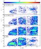 |
Fig. C.1 Density maps for asteroids according to their classification, considering all proper eccentricities. a) Cp/Xp asteroids with WISE albedo pV> 0.1; b) Cp/Xp asteroids with WISE albedo pV< 0.1; c) all Cp/Xp asteroids; d) all Sp asteroids. |
We can then directly compare this distribution (Fig. C.1c) with the distribution of the volatile-poor Sp-complex asteroids (Fig. C.1d). From such a comparison, is clear that the Cp/Xp asteroids are more evenly distributed in the MB, while in the outer belt the Sp-complex are present mostly around the 158 Koronis and 221 Eos families. Also, the Cp/Xp asteroids seem to dominate the inner MB for proper inclinations Ip> 7o.
Appendix D: Dynamical maps and mean-motion resonances
The construction of dynamical maps on the representative (aosc, Iosc)-planes of the osculating elements is based on the spectral analysis method (SAM) described in Michtchenko et al. (2002). For each eccentricity interval, the initial semimajor axes and inclinations of the massless test particles were distributed over a rectangular grid, covering the representative plane with the spacings Δaosc = 0.002 AU and ΔIosc = 0.1°. The initial value of the eccentricity was fixed at the mean value of the corresponding eccentricity interval, while the initial angular elements, Ω,ϖ, and λ, have been chosen aleatory. Each particle has been integrated over 4.2 Myr, accounting for planetary perturbations from Mars to Neptune. During the integration, a low pass-band digital filter has been applied to remove the short-period oscillations on the order of orbital and synodic periods.
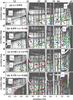 |
Fig. D.1 Dynamical maps on the (a, I)-planes of the osculating semimajor axis and inclination. The gray color levels indicate stochasticity of motion: lighter regions corresponds to regular motion, while darker tones indicate increasingly chaotic motion. The hatched regions correspond to initial conditions that lead to the escape of objects within 4.2 Myr. The large objects from the corresponding eccentricity interval are superposed on each graph: Red stars are objects with diameters D> 100 km, green stars are objects with D in the range from 50 km to 100 km, and blue stars are objects with 30 km <D< 50 km. |
For each test orbit, the output series of filtered elements have been Fourier analyzed to identify the relevant peaks in their Fourier spectra. The number of the relevant peaks in the semimajor axis variation, known as a “spectral number N”, was used to characterize the chaoticity of the orbit: for regular orbits with small values of N, a few well-defined lines appear in the spectra, while for chaotic orbits the number of peaks (consequently, N) is huge. Using a gray scale code, this information is plotted on the representative (aosc, Iosc)-planes of the osculating semimajor axis and inclination.
Figures D.1 and D.2 show the dynamical maps of the MB plotted on the planes corresponding to the different eccentricity intervals. Lighter regions on the dynamical maps correspond to regular motion, and darker tones indicate increasingly chaotic motion. The domains, where the test particles escape within the time span of integration (~4.2 Myr), are hatched. On the dynamical maps we superpose proper elements of some real objects from the corresponding eccentricity range. Only larger objects are shown; those with diameters D> 100 km are indicated with red stars, those with 50 km<D< 100 km are indicated with green stars, and those with 30 km<D< 50 km are indicated with blue stars. It is worth emphasizing that the dynamical map constructed over a grid of osculating orbital elements cannot be directly compared to the proper elements of the asteroids; thus, Figs. D.1 and D.2 provide only an estimation of the dynamical distribution of large objects in the MB.
The dominant effects on the asteroidal motion are produced by the linear SRs, ν5, ν6, and ν16. These resonances are responsible for large-scale instabilities followed by the rapid escape of the test particles from the MB. They also define natural borders of the MB (Williams & Faulkner 1981; Froeschlé & Scholl 1989). The ν6 resonance crosses all maps, from the lower-left to the upper-right corners in Figs. D.1 and D.2. The main bulk of real objects is located below this resonance and forms the low-inclination population of the MB. The ν5 resonance produces the large domains of chaotic motion in the high inclination zones and defines an upper boundary of the asteroidal population of the MB. High inclination domains of quasi-regular motion (light colored) can be observed between the ν5 and ν6 resonances on all panels in Figs. D.1 and D.2. Finally, the ν16 SR occurs at high inclinations and, together with the ν6 resonances, defines the left-side border of the MB.
A relevant feature clearly visible in Figs. D.1 and D.2 is the occurrence of several vertical strips of highly chaotic motion (hatched regions), which are associated with the low-order, MMRs with Jupiter. At low-eccentricity domains, the dominating MMRs are the 3/1, 5/2, 7/3, and 2/1 MMRs with Jupiter, whose chaotic regions are characterized by rapid ejection of the test particles from the MB. At increasing eccentricities, the 8/3 and 9/4 MMRs with Jupiter become strong and effective in fast removing the particles from the region. The devastating effects of the 2/1 MMR create the natural right-side boundary of the MB at ap ≃ 3.3 AU. Beyond this boundary, only the objects from the Hilda group and the Trojans, whose dynamical stability is protected by the 3/2 and 1/1 MMRs with Jupiter, respectively, survive the proximity to the major planet of the solar system.
Apart the strong MMRs with Jupiter, there are many high-order, two-body, and three-body resonances with the planets from Mars to Uranus (e.g., Gallardo 2014). They appear as black vertical strips in Figs. D.1 and D.2. These resonances are weak in the inner belt as a result of the large distance from the Jupiter-Saturn system and the small mass of Mars. In contrast, they are strong in the outer belt because of their proximity to the Jupiter-Saturn system, which makes them very important in removing the objects from the belt. The list of the main two- and three-body MMRs is present in Table A.1 in Appendix A. With increasing eccentricities, the MMRs become stronger, their widths are growing, raising the resonance overlap and, consequently, the increasing instabilities, clearly seen in the very high-eccentricity domain in Fig. D.2. Despite this, an appreciable number of the large objects is still observed at these eccentricities, mainly in the middle zone of the MB.
Appendix E: Density maps of chaotic MB objects
To relate the features of the dynamical maps to the dynamical stability of the real objects, we construct the density maps of the chaoticity of these objects. Using the information on chaoticity provided by the values of LCE (maximum Lyapunov characteristic exponents) in the AstDyS-catalog, we separate our sample in two groups. The first group contains the objects with Lyapunov times (inverse of LCE) longer than 25 000 years and we arbitrarily associate this value with quasi-regular motion and “stable chaos” (Knežević & Milani 2000). The second group consists of the objects with Lyapunov times <25 000 years; this value is associated with unstable motion.
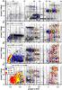 |
Fig. E.1 Density maps of the chaotic MB objects. The location of the main MMRs is indicated with vertical lines and the location of the linear ν6 SR is shown with thick curves. The objects from the AstDyS–catalog are shown with black dots in the background. |
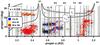 |
Fig. E.2 Same as in Fig. E.1, except in the very high-eccentricity interval extended to Ip = 35° on the representative (ap, Ip)–plane. |
Figures E.1 and E.2 show the density index of unstable objects defined as a fraction (in per cent) of the chaotic asteroids (with Lyapunov times <25 000 years) in the sample inside the cells of the dimension on the (ap, Ip)-plane. For the sake of comparison with Figs. 2 and 3, the only cells with the sample of more than five objects are shown. The density of chaotic objects varies in the three intervals: low (from 5% to 20%, blue), moderate (between 20% and 50%, yellow), and high (above 50%, red). To associate the occurrence of chaotic behavior with the action of the MMRs, we show the web of the main MMRs by vertical lines. On all graphs, the real objects from the corresponding eccentricity interval are shown with black dots in the background.
The correspondence between the MMRs and chaos is clearly observed in Figs. E.1 and E.2. There are gaps of the real objects around the 3/1, 5/2, 7/3, and 2/1 MMRs with Jupiter because of the highly chaotic behavior of the objects and their rapid ejections from these regions. On the other hand, there is a considerable amount of actual unstable objects associated with weaker two- and three-body MMRs, which are concentrated preferably in the outer zone of the MB at all eccentricities (Knezevic & Milani 2000). The number of chaotic asteroids around the MMRs are enhanced with increasing eccentricities as seen in Fig. E.2. The boomerang-like structure is very slightly affected by instabilities raised by MMRs, even in the very high-eccentricity region.
The high-order two- and three-body resonances are weak in the inner zone of the MB, where only the 7/2 MMR with Jupiter and the 1/2 MMR with Mars (at ~2.42 AU) produce some significant effects on the asteroidal motion. The distribution of the unstable orbits in this region is visibly different from that observable in the middle and outer belts. This is because unstable asteroidal motions in the inner belt are originated mainly by the SRs, which are linear and nonlinear (Alvarez-Candal et al. 2006; Michtchenko et al. 2010). The effects of the SRs increase with increasing eccentricities and become visible at ep> 0.125. In the high-eccentricity region (graph d in Fig. E.1), the number of the chaotic objects reaches about a half of the whole population and this value increases to 82% at the very high eccentricities (Fig. E.2). However, in the very high-eccentricity region of the outer belt, where the high-order, two- and three-body MMRs are dense and strong, the same index (obtained over the nearly similar number of the objects) is equal to 64%.
Appendix F: Main families and clusters in the MB
The list of the main nominal families and clusters in the MB obtained with the classical hierarchical clustering method (Zappalá et al. 1990) is shown in Table F.1.
Main nominal families and clusters in the MB obtained with the classical hierarchical clustering method.
All Tables
Main nonlinear SRs, present in the region of the asteroidal belt below the ν6 SR.
Main nominal families and clusters in the MB obtained with the classical hierarchical clustering method.
All Figures
|
Fig. 1 Top: number of MB objects as a function of the absolute magnitude in logarithmic scale. The different colors show different zones of the asteroid belt. Bottom: the two-sample Kolmogorov-Smirnov test; the red curve indicates the middle-inner belt comparison, while the black curve indicates the outer-inner belt comparison (for details, see text). |
| In the text | |
|
Fig. 2 Density distribution of MB objects in the proper (ap, Ip) element space limited to Ip ≤ 20°. Only objects with absolute magnitudes below 15.5 were considered. The eccentricity interval shown on the top of each graph. The density or number (in per cent) of the asteroids inside a cell is shown with different colors (see the legend box); blue corresponds to minimal values (between 2 and 5) and red to maximal values (>20). The size of the cell is |
| In the text | |
|
Fig. 3 Same as in Fig. 2, except in the very high-eccentricity interval extended to Ip = 35° on the representative (ap, Ip)-plane. |
| In the text | |
|
Fig. 4 Frequency distribution of MB objects (normalized to total amount) in the proper semimajor axes (top), proper eccentricities (middle), and proper inclinations (bottom). Gray patterns: general background population of the MB (for details, see text). Red patterns: large objects (D> 30 km). Solid vertical lines show the current location of the strong Jovian MMRs. Their location until the sweeping by migrating Jupiter is shown by dashed vertical lines. |
| In the text | |
|
Fig. 5 Comparison between the distribution of volatile-poor (red) and volatile-rich (blue) objects with diameters, D, larger than: a) 300 km; b)200 km; c) 100 km; and d) 50 km. |
| In the text | |
|
Fig. 6 Density maps for Sp asteroids, considering proper eccentricities intervals: a) – ep< 0.075; b) – 0.075 <ep< 0.125; c) – 0.125 <ep< 0.175; and d) – 0.175 <ep< 0.225. |
| In the text | |
|
Fig. 7 Density maps for Cp/Xp asteroids, considering proper eccentricities intervals: a) – ep< 0.075; b) – 0.075 <ep< 0.125; c) – 0.125 <ep< 0.175; and d) – 0.175 <ep< 0.225. |
| In the text | |
|
Fig. 8 Density maps for asteroids with proper eccentricities ep> 0.225, according to their taxonomy classification. a) Cp/Xp asteroids; b)Sp asteroids. |
| In the text | |
|
Fig. 9 Averaged dynamical maps in the proper elements space limited to Ip< 20°. The red dots are averaged orbital elements of the test particles, whose behavior is affected by MMRs and nonlinear SRs. The black dots are proper elements of the objects from the AstDyS-catalog. The location of the main MMRs is sketched by vertical lines, while the main nonlinear SRs are indicated by the group number from Table A.2. |
| In the text | |
|
Fig. 10 Same as in Fig. 9, except in the very high-eccentricity interval extended to Ip = 35° on the representative (ap, Ip)-plane. |
| In the text | |
|
Fig. 11 Sketch of the main MMRs (vertical lines) and the strong linear and nonlinear SRs (solid curves) in the MB. The nonlinear SRs are identified by the group number from Table A.2. The dots indicate proper elements of the objects within the corresponding eccentricity interval from the AstDyS catalog. The large objects from the corresponding eccentricity interval are superposed on each graph: red stars indicate objects with diameters D> 100 km, green stars indicate objects with D in the range from 50 km to 100 km, and blue stars indicate objects with 30 km <D< 50 km. |
| In the text | |
|
Fig. 12 Same as in Fig. 11, except in the very high-eccentricity interval extended to Ip = 35° on the representative (ap, Ip)–plane. |
| In the text | |
|
Fig. 13 Comparative distribution of the background objects in the inner MB (gray patterns), middle MB (red line), and outer MB (black line). Top: in the proper eccentricities. Bottom: in the proper inclinations. |
| In the text | |
|
Fig. 14 Frequency distribution of the initially uniformly distributed along the semimajor axis objects with the radius of 1000 m, after 2 × 10⁵ yr (gray) and 1.2 × 10⁹ yr (red) of the evolution under perturbations of the five planets and Yarkovsky effects. |
| In the text | |
|
Fig. B.1 An overview of the MB objects on the four representative (ap, Ip)-planes. |
| In the text | |
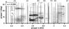 |
Fig. B.2 Same as in Fig. B.1, except for the very high-eccentricity objects. |
| In the text | |
|
Fig. C.1 Density maps for asteroids according to their classification, considering all proper eccentricities. a) Cp/Xp asteroids with WISE albedo pV> 0.1; b) Cp/Xp asteroids with WISE albedo pV< 0.1; c) all Cp/Xp asteroids; d) all Sp asteroids. |
| In the text | |
|
Fig. D.1 Dynamical maps on the (a, I)-planes of the osculating semimajor axis and inclination. The gray color levels indicate stochasticity of motion: lighter regions corresponds to regular motion, while darker tones indicate increasingly chaotic motion. The hatched regions correspond to initial conditions that lead to the escape of objects within 4.2 Myr. The large objects from the corresponding eccentricity interval are superposed on each graph: Red stars are objects with diameters D> 100 km, green stars are objects with D in the range from 50 km to 100 km, and blue stars are objects with 30 km <D< 50 km. |
| In the text | |
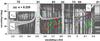 |
Fig. D.2 Same as in Fig. D.1, except in the very high-eccentricity interval e> 0.225. |
| In the text | |
|
Fig. E.1 Density maps of the chaotic MB objects. The location of the main MMRs is indicated with vertical lines and the location of the linear ν6 SR is shown with thick curves. The objects from the AstDyS–catalog are shown with black dots in the background. |
| In the text | |
|
Fig. E.2 Same as in Fig. E.1, except in the very high-eccentricity interval extended to Ip = 35° on the representative (ap, Ip)–plane. |
| In the text | |
Current usage metrics show cumulative count of Article Views (full-text article views including HTML views, PDF and ePub downloads, according to the available data) and Abstracts Views on Vision4Press platform.
Data correspond to usage on the plateform after 2015. The current usage metrics is available 48-96 hours after online publication and is updated daily on week days.
Initial download of the metrics may take a while.