| Issue |
A&A
Volume 587, March 2016
|
|
|---|---|---|
| Article Number | A80 | |
| Number of page(s) | 22 | |
| Section | Cosmology (including clusters of galaxies) | |
| DOI | https://doi.org/10.1051/0004-6361/201527670 | |
| Published online | 22 February 2016 | |
CLASH-VLT: A highly precise strong lensing model of the galaxy cluster RXC J2248.7−4431 (Abell S1063) and prospects for cosmography
1 Dipartimento di Fisica e Scienze della Terra, Università degli Studi di Ferrara, via Saragat 1, 44122 Ferrara, Italy
2 Dark Cosmology Centre, Niels Bohr Institute, University of Copenhagen, Juliane Maries Vej 30, 2100 Copenhagen, Denmark
3 University Observatory Munich, Scheinerstrasse 1, 81679 Munich, Germany
4 INAF–Osservatorio Astronomico di Trieste, via G. B. Tiepolo 11, 34143 Trieste, Italy
5 Kapteyn Astronomical Institute, University of Groningen, Postbus 800, 9700 AV Groningen, The Netherlands
6 Dipartimento di Fisica, Università degli Studi di Milano, via Celoria 16, 20133 Milano, Italy
7 INAF–Osservatorio Astronomico di Capodimonte, via Moiariello 16, 80131 Napoli, Italy
8 INAF–Osservatorio Astrofisico di Arcetri, Largo E. Fermi, 50125 Firenze, Italy
9 Cahill Center for Astronomy and Astrophysics, California Institute of Technology, MS 249-17, Pasadena, CA 91125, USA
10 Dipartimento di Fisica, Università degli Studi di Trieste, via G. B. Tiepolo 11, 34143 Trieste, Italy
11 Space Telescope Science Institute, 3700 San Martin Drive, Baltimore, MD 21208, USA
12 Center for Cosmology and Astro-Particle Physics, The Ohio State University, Columbus, OH 43210, USA
13 Department of Physics, The Ohio State University, Columbus, OH 43210, USA
14 INAF–Osservatorio Astronomico di Bologna, via Ranzani 1, 40127 Bologna, Italy
15 INFN–Sezione di Bologna, viale Berti Pichat 6/2, 40127 Bologna, Italy
16 Institute of Astronomy as Astrophysics, Academia Sinica, PO Box 23-141, Taipei 10617, Taiwan
17 Ikerbasque, Basque Foundation for Science, Alameda Urquijo, 36-5 Plaza Bizkaia, 48011 Bilbao, Spain
18 INAF–Istituto di Astrofisica Spaziale e Fisica cosmica (IASF) Milano, via Bassini 15, 20133 Milano, Italy
19 Department of Astronomy/Steward Observatory, University of Arizona, 933 North Cherry Avenue, Tucson, AZ 85721, USA
20 Laboratoire AIM-Paris-Saclay, CEA/DSM-CNRS-Université Paris Diderot, Irfu/Service d’Astrophysique, CEA Saclay, Orme des Merisiers, 91191 Gif-sur-Yvette, France
21 University of Vienna, Department of Astrophysics, Türkenschanzstr. 17, 1180 Wien, Austria
22 Max Planck Institute for Extraterrestrial Physics, Giessenbachstrasse, 85748 Garching, Germany
⋆
Corresponding author: G. B. Caminha, e-mail: gbcaminha@fe.infn.it
Received: 30 October 2015
Accepted: 14 December 2015
Aims. We perform a comprehensive study of the total mass distribution of the galaxy cluster RXC J2248.7−4431 (z = 0.348) with a set of high-precision strong lensing models, which take advantage of extensive spectroscopic information on many multiply lensed systems. In the effort to understand and quantify inherent systematics in parametric strong lensing modelling, we explore a collection of 22 models in which we use different samples of multiple image families, different parametrizations of the mass distribution and cosmological parameters.
Methods. As input information for the strong lensing models, we use the Cluster Lensing And Supernova survey with Hubble (CLASH) imaging data and spectroscopic follow-up observations, with the VIsible Multi-Object Spectrograph (VIMOS) and Multi Unit Spectroscopic Explorer (MUSE) on the Very Large Telescope (VLT), to identify and characterize bona fide multiple image families and measure their redshifts down to mF814W ≃ 26. A total of 16 background sources, over the redshift range 1.0−6.1, are multiply lensed into 47 images, 24 of which are spectroscopically confirmed and belong to ten individual sources. These also include a multiply lensed Lyman-α blob at z = 3.118. The cluster total mass distribution and underlying cosmology in the models are optimized by matching the observed positions of the multiple images on the lens plane. Bayesian Markov chain Monte Carlo techniques are used to quantify errors and covariances of the best-fit parameters.
Results. We show that with a careful selection of a large sample of spectroscopically confirmed multiple images, the best-fit model can reproduce their observed positions with a rms scatter of 0.̋3 in a fixed flat ΛCDM cosmology, whereas the lack of spectroscopic information or the use of inaccurate photometric redshifts can lead to biases in the values of the model parameters. We find that the best-fit parametrization for the cluster total mass distribution is composed of an elliptical pseudo-isothermal mass distribution with a significant core for the overall cluster halo and truncated pseudo-isothermal mass profiles for the cluster galaxies. We show that by adding bona fide photometric-selected multiple images to the sample of spectroscopic families, one can slightly improve constraints on the model parameters. In particular, we find that the degeneracy between the lens total mass distribution and the underlying geometry of the Universe, which is probed via angular diameter distance ratios between the lens and sources and the observer and sources, can be partially removed. Allowing cosmological parameters to vary together with the cluster parameters, we find (at 68% confidence level) Ωm = 0.25+ 0.13-0.16 and w = −1.07+ 0.16-0.42 for a flat ΛCDM model, and Ωm = 0.31+ 0.12-0.13 and ΩΛ = 0.38+ 0.38-0.27 for a Universe with w = −1 and free curvature. Finally, using toy models mimicking the overall configuration of multiple images and cluster total mass distribution, we estimate the impact of the line-of-sight mass structure on the positional rms to be 0.̋3 ± 0. We argue that the apparent sensitivity of our lensing model to cosmography is due to the combination of the regular potential shape of RXC J2248, a large number of bona fide multiple images out to z = 6.1, and a relatively modest presence of intervening large-scale structure, as revealed by our spectroscopic survey.
Key words: galaxies: clusters: individual: RXC J2248.7-4431 / gravitational lensing: strong / cosmological parameters / dark matter
© ESO, 2016
1. Introduction
Different cosmological probes agree on the finding that the total energy density of the present Universe is composed of less than 5% ordinary baryonic matter; approximately 20% a poorly understood form of non-relativistic matter, called dark matter; and more than 70% an enigmatic constituent with negative pressure (i.e., with an equation of state of the form P = wρ, where P and ρ are the pressure and the density, respectively, and w is a negative quantity), called dark energy. This dark energy component can account for the current epoch of accelerating expansion of the Universe (e.g. Riess et al. 1998; Perlmutter et al. 1999; Efstathiou et al. 2002; Eisenstein et al. 2005; Komatsu et al. 2011; Planck Collaboration XVI 2014).
The combination of both geometrical probes and statistics depending on the cosmic growth of structure, e.g. the cluster mass function or the matter power spectrum, has long been recognized as critical in the effort to measure the global geometry of the Universe and test theories of gravity at the same time. In this context, gravitational lensing is a powerful astrophysical tool that can be used to investigate the global structure of the Universe. The matter distribution at different scales and cosmic epochs can be probed with cosmic shear techniques. Both weak and strong lensing methods are very effective in measuring the mass distribution of dark matter halos on galaxy and cluster scales. In addition, the observed positions and time delays of multiple images of strongly lensed sources are sensitive to the geometry of the Universe. In fact, these observables depend on the angular diameter distances between the observer, lens, and source, and, thereby, one can in principle constrain cosmological parameters as a function of redshift, which describes the relative contributions to the total matter-energy density (see e.g. Schneider et al. 1992).
On galaxy scales, detailed strong lensing models of background, multiply-imaged quasars (e.g. Suyu et al. 2010, 2013) and sources at different redshifts (e.g. Collett & Auger 2014), and analyses of statistically significant samples of strong lenses (e.g. Grillo et al. 2008; Schwab et al. 2010) have shown promising results that can complement those of other cosmographic probes and test their possible unknown systematic effects. On galaxy cluster scales, it has only recently been possible to exploit the observed positions of spectroscopically confirmed families of multiple images to obtain precise measurements of the total mass distributions in the core of these lenses (e.g. Halkola et al. 2008; Grillo et al. 2015b) and the first constraints on cosmological parameters (e.g. Jullo et al. 2010; Magaña et al. 2015). In the last few years, there has been a significant improvement in the strong lensing modelling of galaxy clusters, based on Hubble Space Telescope (HST) multi-colour imaging, used to identify and measure with high precision the angular positions of the multiple images, and deep spectroscopy, which secures the redshifts of lensed sources and cluster members.
The HST Multi-Cycle Treasury Program Cluster Lensing And Supernova survey with Hubble (CLASH; P.I.: M. Postman; Postman et al. 2012a) and the Director Discretionary Time programme Hubble Frontier Fields1 (HFF; P.I.: J. Lotz) have led to the identification of hundreds of multiple images, deflected and distorted by the gravitational fields of massive galaxy clusters. Their apparent positions have been measured with an accuracy lower than an arcsecond and their morphologies well characterized. The spectroscopic redshifts of many of these systems have been obtained as part of a separate Very Large Telescope (VLT) spectroscopic follow-up campaigns with the VIsible Multi-Object Spectrograph (VIMOS; Le Fèvre et al. 2003) and the Multi Unit Spectroscopic Explorer (MUSE; Bacon et al. 2010). In particular, the ESO Large Programme 186.A−0798 (P.I.: P. Rosati; Rosati et al. 2014), the so-called CLASH-VLT project (hereafter just CLASH-VLT), has provided an extensive spectroscopic data set on several of these galaxy cluster lenses.
In this paper, we focus on the HFF cluster RXC J2248.7−4431 (or Abell S1063; hereafter RXC J2248), which was part of the CLASH survey. The clusters sample selection and observations are presented in Maughan et al. (2008) and Gilmour et al. (2009). We take advantage of our CLASH multi-band HST data and extensive spectroscopic information, which we have collected on the cluster members and background lensed sources in this galaxy cluster with the VIMOS and MUSE instruments at the VLT (see Balestra et al. 2013; Karman et al. 2015). Combining the HST and VLT data sets, we develop a highly accurate strong lensing model, which is able to constrain the mass distribution of the lens in the inner region and, at the same time, provides interesting constraints on the cosmological parameters, which are ultimately limited by the intervening large-scale structure along the line of sight and the model assumptions on the mass distribution.
When not specified, the computations were made considering a flat ΛCDM cosmology with Ωm = 0.3 and H0 = 70 km s-1 Mpc-1. In this cosmology, 1′′ corresponds to a physical scale of 4.92 kpc at the cluster redshift (zlens = 0.348). In all images north is top and east is left.
2. RXC J2248
RXC J2248 is a rich galaxy cluster at zlens = 0.348 and was first identified as Abell S1063 in Abell et al. (1989). The high mass and redshift of RXC J2248 make it a powerful gravitational lens creating several strong lensing features, such as giant arcs, multiple image families and distorted background sources. As detailed in this article, a total of 16 multiple image families, ten of which are spectroscopically confirmed, have been securely identified to date over an area of 2 arcmin2. RXC J2248 was one of the 25 clusters observed within CLASH (Postman et al. 2012a) in 16 filters, from the UV through the near-IR with the ACS and WFC3 cameras on board HST. The full-depth, distortion-corrected HST mosaics in each filter were all produced using procedures similar to those described in Koekemoer et al. (2011), including additional processing beyond the default calibration pipelines and astrometric alignment across all filters, to a precision better than a few milliarcseconds.
In Fig. 1, we show a colour image of RXC J2248 obtained from the combination of the CLASH ACS and WFC3 filters. The red circles indicate the position of the multiple images with spectroscopic redshift, the magenta circles designate families with no spectroscopic confirmation, while the white circles indicate sources close to cluster members or possibly lensed by line-of-sight mass structures or not secure counter images. The positions of the multiple images are uniformly distributed around the cluster core, providing constraints on the overall cluster mass distribution. Most of the families are composed of two or three multiple images, except for the family at redshift 6.111 (ID 14), which is composed of five identified images (see Balestra et al. 2013; Monna et al. 2014). After the submission of this paper, deeper HST imaging from the HFF programme became available, allowing us to detect a fifth, faint image (ID 14e) close to the BCG (see Fig. 6). The spectroscopic confirmation of the redshift of this multiple image will be given in Karman et al. (in prep.). As a result of the late identification of image 14e, we include it in only one strong lensing model, labelled as F1-5th in Table 4. We anticipate that the high redshift of this source and its multiple image configuration, similar to an Einstein’s cross, will play an important role in constraining the cluster total mass distribution and the relation between angular diameter distances and redshifts (for more details, see Sect. 4).
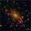 |
Fig. 1 Colour composite image of RXC J2248 obtained using the 16 HST/ACS and WFC3 filters. Spectroscopically confirmed multiple images are indicated in red; multiple images with no spectroscopic redshift in magenta. White circles indicate sources close to a cluster member, or possibly lensed by line-of-sight structures, or with not secure counter images. These last images are not used in the lens model. More information is provided in Table 1. The blue circle shows the position of the BCG. The multiple image ID 14e is only used in the model F1-5th; see Table 4. |
The total mass distribution of RXC J2248 has been studied with different probes, such as X-ray emission (Gómez et al. 2012) and strong (Monna et al. 2014; Johnson et al. 2014; Richard et al. 2014; Zitrin et al. 2015) and weak lensing analyses (Gruen et al. 2013; Umetsu et al. 2014; Merten et al. 2015; Melchior et al. 2015), with generally good agreement between these different techniques. Gómez et al. (2012) indicates that the galaxy cluster has undergone a recent off-axis merger, and Melchior et al. (2015) find the cluster to be embedded in a filament with corresponding orientation. However, moderately deep X-ray Chandra observations show an elongated but regular shape, with no evidence of massive substructures in the inner region (see Fig. 2).
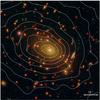 |
Fig. 2 Colour composite image of RXC J2248 overlaid with the Chandra X-ray contours in white (Gómez et al. 2012). Red circles indicate the selected cluster members (see Sect. 3.1.2). The magenta circle shows the second brightest cluster member, used as the reference for the normalization of the mass-to-light ratio of the cluster members, i.e. L0 in Eq. (3). |
Previous strong lensing analyses (Monna et al. 2014; Johnson et al. 2014; Richard et al. 2014) have shown that the cluster total mass distribution of RXC J2248 can be well represented by a single elliptical dark matter halo with the addition of the galaxy cluster members. These studies have suggested that the dark matter halo has a significantly flat core of ≈17′′. The influence of the BCG during the cluster merging process (e.g. Laporte & White 2015) and baryonic physics effects (e.g. Tollet et al. 2016) can account for the formation of a core in the dark-matter density distribution of clusters and galaxies. However, more simulations should be explored to better characterize these effects in objects with different formation histories and mass scales.
The regular shape and lens efficiency of RXC J2248, in combination with high quality multi-colour imaging and extensive spectroscopy measurements, makes it a very suitable system for testing high-precision strong lensing modelling of the mass distribution of galaxy clusters with appreciable leverage on the underlying geometry of the Universe.
Upcoming deeper observations of this cluster via the Grism Lens-Amplified Survey from Space (GLASS; GO-13459; P.I.: T. Treu, Treu et al. 2015), the HFF campaign and MUSE, are expected to further increase the number of identified multiple image families and spectroscopic confirmations.
2.1. VIMOS observations and data reduction
As part of the CLASH-VLT Large programme, the cluster RXC J2248 was observed with the VIMOS spectrograph between June 2013 and May 2015. The VIMOS slit-masks were designed in sets of four pointings with one of the quadrants centred on the cluster core and the other three alternatively displaced in the four directions (NE, NW, SE, SW). A total of 16 masks were observed, 12 with the low-resolution (LR) blue grism, and four with the intermediate-resolution (MR) grism; each mask was observed for either 3 × 20 or 3 × 15 min (15 h exposure time in total). Therefore, the final integration times for arcs and other background galaxies varied between 45 min and 4 h. A summary of our VIMOS observations is presented in Table 2. We used 1″-slits. The LR-blue grism has a spectral resolution of approximately 28 Å and a wavelength coverage of 3700−6700 Å, while the MR grism has a spectral resolution of approximately 13 Å and it covers the wavelength range 4800−10 000 Å.
We define four quality classes by assigning a quality flag (QF) to each redshift measurement, which indicates the reliability of a redshift estimate. The four quality classes are defined as follows: secure (QF = 3), likely (QF = 2), insecure (QF = 1), and based on single emission line (QF = 9). Duplicate observations of hundreds of sources across the whole survey allow us to quantify the reliability of each quality class as follows: redshifts with QF = 3 are correct with a probability of >99.99%, QF = 9 with ~92% probability, QF = 2 with ~75% probability, and QF = 1 with <40% probability. In this paper we only consider redshifts with QF = 3, 2, or 9. A total of 3734 reliable redshifts were measured over a field ~25 arcmin across, where 1184 are cluster members and 2425 are field galaxies (125 are stars). For a complete description of the data acquisition and reduction, see Balestra et al. (in prep.) and Rosati et al. (in prep.).
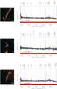 |
Fig. 3 VLT/VIMOS spectra of the multiple image systems. Left panels: HST cutouts, 10′′ across with the position of the VIMOS 1′′-wide slits and the image ID from Table 1. One- and two-dimensional spectra are shown on the right with measured redshifts and quality flags, including typical emission and absorption lines. |
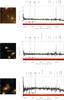 |
Fig. 3 continued. |
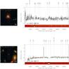 |
Fig. 3 continued. |
In Fig. 3, we show the spectra of the multiply imaged sources. On the left, we show the HST cutout with the position of the 1″-wide slit of VIMOS. On the right, the one- and two-dimensional spectra with the estimated redshifts and quality flags are shown. All spectra present clear emission lines, ensuring reliable redshifts for most of the measurements, i.e. QF=3, with the exception of the low S/N spectrum of image 8a (QF=9), however, its redshift of z = 1.837 is confirmed by MUSE observations (see Sect. 2.2).
The positions and redshift values (zspec) of all multiple image families are given in Table 1; positions and redshift values of magnified sources that are not multiply lensed are given in Table 3. We also quote the Kron observed magnitudes of each source measured with SExtractor (Bertin & Arnouts 1996) in the F814W filter. We use our strong lensing model F2 (see Table 4 and Sect. 4) to compute the best-fit value of the redshift (zmodel) of all multiply imaged sources not spectroscopically confirmed and to compute the magnification factors (μ). The value of μ is computed for a point-like object at the position of the images. Since the model F2 is not suitable to compute the magnification of the families 8, 11 and multiple image 3b, we quote the magnifications values given by the model that includes all spectroscopically confirmed multiple images (model ID F1a, see Table 4). For family 11, which presents two multiple images very close to the tangential critical line and the highest offset between the observed and model-predicted positions ( ), we quote the magnification values at the model-predicted positions. These values are less sensitive to the systematic effects affecting this family and are discussed in Sect. 3.4.
Magnitudes corrected by the magnification factor ( ) are also estimated. The apparent disagreement in the values of of some multiple image families can be the result of the evaluation of μ, which is computed in a point and not integrated over the extended image, and the difficulties in the photometric measurement of highly extended images, such as the multiple images of the families 2 and 3. The high magnification efficiency of RXC J2248 allows us to probe spectroscopically the very faint end of the galaxy luminosity function at high redshift with intrinsic unlensed magnitudes extending down to M1600 ≈ −15, i.e. approximately 5 mag below M∗ (Bouwens et al. 2011).
2.2. MUSE redshift measurements
Observations with the new integral-field spectrograph MUSE on the VLT were conducted in the south-west part of the cluster as part of the MUSE science verification programme (ID 60.A-9345, P.I.: K. Caputi). A 8520 s total exposure was obtained in June 2014 with a seeing of ≈1″. The MUSE data cube covers 1 × 1 arcmin2 with a pixel size of  , over the wavelength range 4750−9350 Å, and with a spectral resolution of ≈3000 and a dispersion of 1.25 Å/pixel. Details on data reduction and results can be found in Karman et al. (2015). We extracted 1D spectra of the strong lensing features within circles with radius ranging from
  to 2″ to minimize the contamination of nearby objects and maximize the signal to noise. In this work, guided by the strong lensing model predictions, we revisited several spectra and measured redshifts of two additional multiple image families not included in the CLASH-VLT data and Karman et al. (2015). In the Figs. 4 and 5, we show the MUSE spectra of the multiple images 8a/b and 20a/b. The spectra of both sources 8a and 8b show a pair of emission lines at the same wavelengths, which we identify as the resolved CIII] doublet (1906.7,1908.7 Å) at z = 1.837. The fact that our lensing models predict these sources to be multiple images at zmodel = 1.81 ± 0.03 lends strong support to this interpretation. Also, the CLASH-VLT spectrum of the source 8a (see Fig. 3, 7th panel) shows an (unresolved) emission line, although it has low S/N (QF = 9).
In Fig. 5 we show the spectra extracted from apertures around the multiple images 20a/b. The existence of an asymmetric emission line at 5007.5 Å is clear, which we identify with a Lyα emission at redshift 3.118. Inspection of the MUSE data cube around this wavelength reveals an extended low-surface brightness emission around each image. The excellent agreement between the modelled redshift of the compact sources (see Table 1) and the extended emission shows that both are related. Based on our lensing model, we interpret this diffuse double emission as two multiply imaged Lyα blobs. LABs are commonly found in deep narrowband image surveys (Fynbo et al. 1999; Steidel et al. 2000; Francis et al. 2001; Nilsson et al. 2006), and their Lyα luminosities are in the range 1043−1044 erg / s with sizes up to ~100 kpc. Although several mechanisms have been proposed to explain their large luminosities, there is still no consensus on the physical nature of these sources (Arrigoni Battaia et al. 2015, and references therein). A detailed study of this source is presented in Caminha et al. (2015).
Multiple image systems.
Log of VIMOS observations of the Frontier Fields cluster RXC J2248, taken as part of the CLASH-VLT spectroscopic campaign.
3. Strong lens modelling
We use the strong lensing observables to reconstruct the total mass distribution of RXC J2248. The positions of the multiple images, from a single background source, depend on the relative distances (observer, lens and source) and on the total mass distribution of the intervening lens. We describe our methodology to determine the mass distribution of the cluster from the observed positions of the identified multiple images below.
First, we visually identify the multiple images on the colour composite HST image (Fig. 1). We revisit all the previously suggested multiple image systems and explore new systems during this identification. Using colour and morphological information of these objects and the expected parity from basic principles of gravitational lensing theory, we select luminosity peaks. In a second step, we refine the measurements with the stacked images of the optical (F435W, F606W, F625W, F775W, F814W and F850lp) and near-IR (F105W, F110W, F125W, F140W and F160W) filters, depending on the colour of the multiple images. However, we do not use different stacked images to measure the luminosity peaks of different multiple images belonging to the same family. We draw different iso-luminosity contours around each peak and determine the position of the centroid of the innermost contour enclosing a few pixels (≈5, or 0.1 square arcsec). With this procedure, we ensure that we consider the peaks of the light distribution of different multiple images that correspond to the same position on the source plane, thus avoiding systematics that are often introduced by automated measurements. The measured positions of multiple images are listed in Table 1.
Magnified but not multiply imaged sources.
Some extended arcs show multiple peaks or knots (e.g. families 2, 4 and 9), thus in principle allowing us to split these families into two subsets, as in Monna et al. (2014). This technique can improve the constraints on the critical lines close to the multiple images, however, it does not introduce any extra constraint in the overall best-fitting model. In this work, we choose to use only one peak for each family to avoid any possible systematic effect in the modelling and to save computational time.
3.1. Mass model components
The optical and X-ray images of the cluster (see Figs. 1 and 2) indicate a regular elliptical shape with no evident large asymmetries or massive substructures in the region where multiple images are formed. In view of its regular shape, we consider three main components for the total mass distribution in the lens modelling: 1) a smooth component describing the extended dark matter distribution; 2) the mass distribution of the BCG; and 3) small-scale halos associated with galaxy members.
We also check whether the presence of an external shear term associated with two mass components in the north-east and south-west of the cluster could improve the overall fit. In these two regions (outside the field of view shown in Fig. 1), we notice the presence of bright cluster galaxies that could contribute to the cluster total mass with additional massive dark matter halo terms. However, we do not find any significant improvement in the reconstruction of the observed positions of the multiple images and these components are completely unconstrained. Moreover, we test a model including an extra mass component in the core of the cluster (R ≲ 300 kpc). Also, in this case the fit does not improve significantly to justify the increase in the number of free parameters, for which we obtain best-fitting values that are physically not very plausible. For example, we find an extremely high value for the mass ellipticity of this new term.
3.1.1. Dark matter component
For the smooth mass component (intra-cluster light, hot gas and, mainly, dark matter) we adopt a pseudo-isothermal elliptical mass distribution (hereafter PIEMD; Kassiola & Kovner 1993). The projected mass density distribution of this model is given by 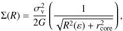 (1)where R(x,y,ε) is an elliptical coordinate on the lens plane and σv is the fiducial velocity dispersion. The ellipticity ε is defined as ε ≡ 1−b/a, where a and b are the semi-major and minor axis, respectively. There are six parameters describing this model: the centre position (x0 and y0), the ellipticity and its orientation angle (ε and θ, where the horizontal is the principal axis and the angle is counted counterclockwise), the fiducial velocity dispersion (σv), and the core radius (rcore). The PIEMD parametrization has been shown to be a good model to describe cluster mass distributions in strong lensing studies and sometimes provides a better fit than the canonical Navarro-Frenk-White (hereafter NFW; Navarro et al. 1996, 1997) mass distribution. Grillo et al. (2015b), using a similar high quality data set, found for example that the dark matter components of the HFF galaxy cluster MACS J0416.1−2403 are better described by PIEMD models.
To test the dependence of our main results on a specific mass parametrization, we also consider an NFW distribution for the main dark matter component. In this work, we use a NFW model with elliptical potential (hereafther PNFW; Kassiola & Kovner 1993; Kneib 2002; Golse & Kneib 2002), which significantly reduces computing time of the deflection angle across the image in the lenstool implementation. For this model, the free parameters are the characteristic radius rs and density ρs, besides the potential ellipticity, orientation angle, and the centre position (ε, θ, x0, and y0). The main differences between these two models are the presence of a core radius in the PIEMD model, while the PNFW has a central cusp and different slopes at large radii.
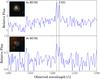 |
Fig. 4 MUSE 1D spectra of the multiple images 8a and 8b. The vertical lines indicate the CIII] doublet emission wavelengths of a source at redshift 1.837. The small panels show the circles with 1″ (top) and |

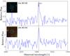 |
Fig. 5 MUSE 1D spectra of the multiple images 20a and 20b. The vertical line indicates the Lyα emission wavelength of a source at redshift 3.118. The small panels show the circles with 1″ radius used to extract the two spectra. The flux is rescaled by a factor of 10-18 erg / s / cm2/Å. |
Summary of the best-fit models.
3.1.2. Cluster members and BCG
Membership selection is performed following the method adopted in Grillo et al. (2015b, see Sect. 3.3.1). Specifically, we investigate the loci, in a multi-dimensional colour space, of a large sample of spectroscopically confirmed cluster members and field galaxies. We define confirmed cluster members as the galaxies within the spectroscopic range of 0.348 ± 0.0135, corresponding to a velocity range of ±3000 km s-1 in the cluster rest frame. We thus find 145 members out of the 254 galaxies with measured redshifts in the HST field of view. We then model the probability density distributions (PDFs) of cluster member and field galaxy colours as multi-dimensional Gaussians, with means and covariances determined using a robust method (minimum covariance determinant; Rousseeuw 1984). This ensures that a small fraction of outliers in colour space (for example, caused by inaccurate photometry, contamination from angularly close objects, or the presence of star-forming regions) does not significantly perturb the measured properties of the PDFs. The colour distribution is traced by all independent combinations of available bands from the 16 CLASH filters with the exclusion of F225W, F275W, F336W, and F390W bands, which often do not have adequate signal-to-noise ratio for red cluster galaxies. For all galaxies, we compute the probability of being a cluster member or a field galaxy, via the determined PDFs in a Bayesian hypotheses inference. We then classify galaxies with a probability threshold that is a good compromise between purity and completeness, and thus select 159 additional cluster members with no spectroscopic redshifts.
In the strong lensing model, we consider only (spectroscopic and photometric) cluster members that are within 1′ radius from the BCG centre, which encloses all the identified multiple images. In this way, we save computational time by not computing the deflection angle of members in the outer regions of the cluster that are not expected to affect the position of the multiple images significantly. Thus, we include 139 cluster members in the model, 64 of which are spectroscopically confirmed.
Each cluster member is modelled as dual pseudo-isothermal elliptical mass distribution (dPIE; Elíasdóttir et al. 2007; Suyu & Halkola 2010) with zero ellipticity and core radius, and a finite truncation radius rcut. The projected mass density distribution of this model is given by 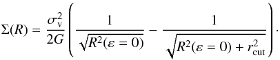 (2)Following a standard procedure in cluster-scale strong lensing analyses (e.g. Halkola et al. 2006; Jullo et al. 2007; Grillo et al. 2015b), to reduce the number of free parameters describing the cluster members, we use the following relations for the velocity dispersion and truncation radius scaling with the luminosity:
 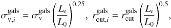 (3)where L0 is a reference luminosity associated with the second most luminous cluster member, which is indicated by the magenta circle in Fig. 2. Given the adopted relations, the total mass-to-light ratio of the cluster members is constant and we reduce the free parameters of all member galaxies to only two parameters: the reference velocity dispersion
  and truncation radius
  . We measure the luminosities (Li) in the F160W band, which is the reddest available filter, to minimize the contamination by blue galaxies around cluster members and to obtain a good estimate of galaxy stellar masses.
Owing to a generally different formation history, the BCG is often observed to deviate significantly from these scaling relations (Postman et al. 2012b). We therefore introduce two additional free parameters associated with the BCG ( and
and  ), keeping its position fixed at the centre of the light distribution.
3.2. Lens modelling definitions
The strong lensing modelling is performed using the public software lenstool (Kneib et al. 1996; Jullo et al. 2007). Once the model mass components are defined, the best-fitting model parameters are found by minimizing the distance between the observed and model-predicted positions of the multiple images, and the parameter covariance is quantified with a Bayesian Markov chain Monte Carlo (MCMC) technique.
In detail, to find the best-fitting model, we define the lens plane χ2 function as follows: 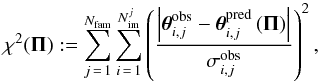 (4)where Nfam and
  are the number of families and number of multiple images belonging to the family j, respectively. The parameters θobs and θpred are the observed and model-predicted positions of the multiple images, and σobs is the uncertainty in the observed position. The model-predicted position of an image is a function of the both lens parameters and cosmological parameters, which are all represented by the vector Π. We adopt flat priors on all parameters, thus, the set of parameters Π that provides the minimum value of the χ2 function (
 ) is called the best-fitting model, while the predicted positions of this model are referred to as θbf. We do not have measured spectroscopic redshifts for some multiple image families. In these cases, the family redshift is also a free parameter optimized in the calculation of the with a flat prior.
Aside from the value of the , we can quantify the goodness of the fit with the root-mean-square between the observed and reconstructed positions of the multiple images: 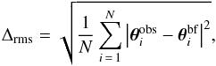 (5)where N is the total number of multiple images. This quantity does not depend on the value of the observed uncertainties σobs, making it suitable when comparing results of different works. Finally, we also define the displacement of a single multiple image i as
 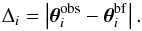 (6)The posterior probability distribution function of the free parameters is given by the product of the likelihood function and the prior
 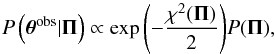 (7)where P(Π) is the prior, which we consider to be flat for all free parameters. We use a MCMC with at least 105 points and a convergence speed rate of 0.1 (a parameter of the BayeSys2 algorithm used by the lenstool software) to properly sample the parameter space and obtain the posterior distribution of the parameter values. We have checked that these values ensure the convergence of the chains. All computations are performed estimating the value of the χ2 function on the image plane, which is formally more accurate than working on the source plane (e.g. Keeton 2001).
3.3. Cosmological parameters
The availability of a large number of multiple images, with spectroscopic redshifts spanning a wide range, in a relatively regular mass distribution, makes RXC J2248 a suitable cluster lens to test the possibility of constraining cosmological parameters. Strong lensing is sensitive to the underlying geometry of the Universe via the angular diameter distances from the observer to the lens (DOL) and source (DOS), and from the lens to the source (DLS). For one source, the lens equation can be written as 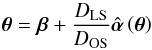 (8)where θ and β are the angular positions on the lens and source planes, respectively,
  is the deflection angle and the cosmological dependence is embedded into the angular diameter distances. In general, the ratio between the cosmological distances can be absorbed by the parameters of the lens mass distribution (i.e. the factor that multiplies the mass distribution), which is
  in the PIEMD case. However, when a significant number of multiply lensed sources at different redshifts is present, this degeneracy can be broken and a leverage on cosmological parameters can be obtained via the so-called family ratio:
 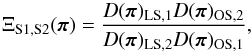 (9)where π is the set of cosmological parameters and 1 and 2 are two different sources at redshifts zs1 and zs2. This technique has been applied in Soucail et al. (2004) and Jullo et al. (2010) for the galaxy clusters Abell 2218 and Abell 1689, respectively. We use the ΛCDM cosmological model, which includes as free parameters the energy density of the total matter of the Universe (ordinary and dark matter) Ωm, the dark energy density ΩΛ and the equation of state parameter of this last component, w = P/ρ. All the results from our lens models are described in Sect. 4.
3.4. Multiple image selection
In the previous strong lensing studies of RXC J2248, 19 candidates of multiple image families were identified (Monna et al. 2014; Johnson et al. 2014; Richard et al. 2014), however, some of them are not secure candidates. The selection of secure multiple image systems, i.e. systems with spectroscopic confirmation or multiple images with correct parity and/or consistent colours, is essential to avoid systematics in lensing models. This criterion leaves us with 16 families, whose properties are summarized in Table 1. Based on this strict criterion, we do not include the counter image 16c in our models, since the corresponding model-predicted position from our best-fitting models (see Sect. 4) is close to two objects with similar colours, leaving the identification of this counter image uncertain.
Given our relatively simple models to parametrize the cluster mass distribution and the total mass-luminosity scaling relation of the cluster members, we also avoid multiple images in the vicinity of the members. Their truncated PIEMD mass with a constant total mass-to-light ratio might not be able to accurately reproduce the positions of the multiple images close to the core of the members, introducing a bias in the best fits. Quantitatively, we do not include multiple images closer than 3 kpc (≈ ) to a cluster member, which is approximately the Einstein’s radius of a galaxy with σv = 160 km s-1 for a source at z = 3. As a result, the multiple images that are not included in our fiducial lens model are 3b, 8a, 8b, and 17b. In the case of family 8, we are left with only one multiple image, which does add any constraint to the models; we therefore exclude the entire family.
Finally, in all different models we analyze, family 11 presents a much larger offset between observed and reconstructed images (Δi ≈ 1″) when compared with the other families (≈ ). We conduct several tests in the effort to improve the fit of this family: 1) we freely vary the mass parameter of the nearby cluster members when optimizing the model. 2) We introduce a dark halo in the vicinity of the images. 3) We consider an external shear component represented by a PIEMD in the south-west region of the cluster with free mass. The third test is suggested by the apparent discontinuity in the X-ray emission from the Chandra data, ~30″ SW of the BCG. We verify that it is difficult to reduce the average value of Δi below 1″ for the images of family 11 by only adding an extra mass component.
We also consider the effect of the large-scale structure along the line of sight, which we can sample with our redshift survey. Specifically, to investigate whether this family could be lensed by a galaxy behind the cluster, we map the positions of the three multiple images onto a plane at the redshift of each background source in the Tables 1 and 3. In this analysis, we find that the background galaxy ID B7 at z = 1.270 (see Table 3) could significantly perturb the positions of the multiple images of family 11, since its distance is ≈25 kpc, or ≈3″, from the positions of the multiple images 11a and 11b on the z = 1.27 plane. In this configuration, assuming a velocity dispersion value of 150 km s-1 for B7, the deflection angle induced in the multiple images of family 11 is ≈ . We therefore argue that the effect of this background galaxy can partially explain the large Δi value of this family, although more complex multi-plane ray-tracing procedures should be employed to fully account for such a deviation. A detailed modelling of the background effects on the strong lensing analyses of RXC J2248 is out of the scope of this work. However, in Sect. 5 we return to this non-negligible issue by estimating the statistical effect on the image positions due to the line-of-sight mass structure, and we show that it can have an important impact on high-precision lensing modelling.
To summarize, in an effort to minimize possible sources of systematic uncertainties, we decide not to include the multiple images 3b, 16c and 17b, and families 8 and 11 in our strong lensing analysis. In the end, we consider a total of 38 multiple images of which 19 are spectroscopically confirmed, belonging to 14 families at different redshifts. We leave the detailed study of individual sources to future work. As the spectroscopic work continues, particularly with VLT/MUSE, we will include a further refinement of the mass distribution modelling, which will take the influence of mass strictures along the line of sight into account.
4. Results
4.1. A collection of lens models
We explore a number of strong lensing models based on different samples of secure multiple-image systems, as described above, and different model parameters.
First we define two samples of multiple-image families: “family sample 1” includes families with spectroscopic confirmation, namely families with IDs 2, 3, 4, 6, 7, 14, and 18, totalling 20 multiple images in seven families; “family sample 2” contains all the secure families, including also multiple images with no spectroscopic confirmation, but with correct colours and parity as expected from gravitational lensing theory. This extended sample includes family IDs 9, 13, 15, 16, 17, 20, and 21 in addition to the seven spectroscopic families, totalling 38 multiple images in 14 families. The redshift of the compact multiple images of family 20 is conservatively considered a free parameter here, since the multiple images are not necessarily associated with the extended Lyα emission (see Sect. 2.2). We find, however, that the best-fit redshift of family 20 obtained from the strong lensing model is in very good agreement with that derived from the LAB emission, confirming a posteriori that the compact sources of family 20 are associated with the extended Lyα emission (see Fig. 5). Since this extra information does not improve the lens models significantly, we did not recompute the MCMC analyses for all the reference models.
To optimize the models, we adopt an image positional error of in the positions of the multiple images, which is in agreement with predictions of the effects of matter density fluctuations along the line of sight on the positions of multiple images (Host 2012). In all cases this choice leads to a  lower than the number of degrees of freedom (d.o.f.; defined as the difference between the number of constraints and the number of free parameters of a model). Positional errors (σobs in Eq. (4)) are then rescaled to yield a value equal to the d.o.f. when probing the space parameter using the MCMC technique. The values of the rescaled σobs are approximately
  for all the models under study. This can effectively account for, e.g. line-of-sight mass structures and the scatter in the adopted total mass-to-light relation of the cluster members.
We exploit different lensing models to assess possible systematic effects stemming from our assumptions on the cluster total mass distribution, multiple image systems and adopted free parameters. A list of all models is given in Table 4, including their main parameters and a brief description of each model.
The IDs of the models are composed of letters indicating the model assumption. The letter “F” indicates a fixed cosmology (flat ΛCDM cosmology with Ωm = 0.3 and H0 = 70 km s-1 Mpc-1), and “N” indicates that we use a PNFW mass profile to represent the smooth dark matter mass distribution instead of a PIEMD. The letter “W” indicates that we vary the parameters Ωm and w (the dark energy equation of state, in a flat Universe) while “L” indicates free Ωm and ΩΛ and fixed w = −1 (i.e. we vary the curvature of the Universe). The letters “WL” indicate we are varying all the three cosmological parameters at the same time. Finally, the ID “Wa” stands for a model where we consider a variation of w with redshift parametrized by w(z) = w0 + waz/ (1 + z).
The numbers in the IDs indicate three different multiple image inputs. The number “1” indicates that we consider only the family sample 1, while “2” refers to all the secure families (family sample 2). Moreover, for two models we also explore the effect of removing the highest redshift source (family 14) on the best-fitting parameters (indicated by “3”). The letter “Z” indicates the models in which we do not use any information on the spectroscopic redshifts, i.e. the redshifts of all families are free parameters in the optimization. For completeness, we also quote results for the model F1a, in which all spectroscopic families are included, i.e. the model F1 with the addition of the families 11 and 8, and image 3b. Although the model F1a has a poor overall fit due to the systematics introduced by the non-bona fide multiple images, it is more accurate to compute lensing quantities, such as the magnification, of these specific multiple images. Finally, after the identification of the fifth image, belonging to family 14 and close to the BCG, we include this image into an additional model. The model F1-5th considers the family sample 1 plus this extra image. We therefore present best-fit models for 22 different cases.
For a subset of models in Table 4, we compute parameter uncertainties by performing a MCMC analysis. Since this can be very time consuming, we do not consider models N1, N2, NW1, and NW2 because they do not accurately describe the properties of the lens mass distribution (see Sect. 4.2). We also exclude the models Wa1 and Wa2 because we find that the multiple image positions are not very sensitive to the variation of the wa parameter. In Table 5, we show the best-fit parameters and their errors (68% confidence level) for the 12 models for which the MCMC analysis was performed (the model IDs refer to Table 4). We do not show the estimated redshift of the family sample 1 for better visualisation for the models FZ1 and FZ2. In the next sections, we discuss the results from the best-fit models on the mass distribution of RXC J2248, the cosmological parameters, and the degree of degeneracy among the different model parameters.
4.2. Mass distribution parameters
Firstly, the PNFW models provide a significantly worse fit than the PIEMD models (compare models F1 and F2 with N1 and N2 in Table 4). The final positional Δrms of N1 and N2 is a factor of 3.5 and 3.9 higher than that of F1 and F2, respectively. The main reason for this difference is that RXC J2248 is characterized by a relatively shallow inner mass density distribution, as pointed out by previous works (Johnson et al. 2014; Monna et al. 2014). Moreover, when we let the values of the cosmological parameters (Ωm and w) to vary in the model optimization, the Δrms is reduced by a factor of 2 for the NW1 and NW2 models. This indicates that a different set of cosmological parameters partially compensates the effects of the presence of a core in the total mass density profile of the cluster. Specifically, we obtain best-fit cosmological parameters Ωm ≈ 0.0 and w < −2.0, which are completely non-physical and in disagreement with other cosmological probes. Moreover, the large Δrms value in this case indicates that this mass distribution profile is such a bad representation of the real profile that the lensing models are unable to probe parameters related to the background cosmology and halo substructures.
By comparing the models with fixed cosmology using the redshift information of the family sample 1, i.e. models F1 and F2 in the Tables 4 and 5, we find that the extra information of the family sample 2 does not significantly change the strong lens modelling. This is indicated by the fact that the Δrms values of these two models are very similar (see Table 4) and the values of all parameters are also consistent within their 1σ confidence levels in Table 5. A larger deviation is obtained for the BCG parameters and , which are not estimated very precisely because the degeneracies with the other parameters and lack of multiple images close to the BCG. This behaviour is present in all the 12 different models we analyzed. We remark that the inclusion of image 14e allows us to obtain a more precise estimate of the value of the effective velocity dispersion of the BCG, but not of its truncation radius. In detail, we find that the median values and 68% confidence levels for these two parameters from the model F1-5th are  km s-1 and
  ″.
″.
Interestingly, the addition of extra families of the sample 2 allows us to reduce the errors on the best-fitting parameters and to place significant constraints on the redshifts of these extra multiple image families. We consider the model F2 as our reference model, since we use the maximum possible and secure information of the clean sample of multiple images. In Fig. 6, we show 4″ wide cutouts of the multiple images used in this model. The red circles have radius and locate the observed input positions listed in Table 1. The yellow crosses are the predicted positions of the lens model F2. All multiple images are very well reproduced by the model and there is no systematic offset in the predicted positions.
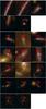 |
Fig. 6 CLASH/HST colour cutouts (4″ wide) of all multiple images used in the reference model F2. Red circles ( |
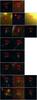 |
Fig. 6 continued. |
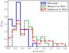 |
Fig. 7 Distribution of the displacement values of the multiple images (absolute values of the observed minus the reconstructed positions, see Eq. (6)) obtained from our reference model F2 (solid blue line) and in previous works by Monna et al. (2014; green dashed) and Johnson et al. (2014; red long dashed), for the cluster RXC J2248. |
In Fig. 7, we compare the distribution of the displacements of each multiple image (Δi, see Eq. (6)) of the reference model F2 with those relative to the multiple images considered in Monna et al. (2014) and Johnson et al. (2014) (the only studies that made this information available). This figure shows that our model reproduces the multiple image positions with better accuracy compared to previous works. Specifically, the final Δrms (Eq. (5)) of our model is  , while is
  in Monna et al. (2014) and
  in Johnson et al. (2014). This difference can be explained by different assumptions in each modelling, such as extra dark matter halos and different cluster member selections, slightly distinct multiple image families, and different redshift information.
We can compare the projected total mass values within an aperture of 250 kpc from these studies. Using the 1σ confidence level of our F2 model, we find  (the errors are given by the 68% confidence level), which is somewhat higher than the values of
  and
and  presented in Johnson et al. (2014) and Monna et al. (2014), respectively. Although these measurements are not consistent within the estimated errors, the mean values do not differ more than 10%, and are likely due to different assumptions in these studies, and aforementiond systematics arising from a non-bona fide set of multiple images.
Since strong lensing modelling in galaxy clusters is often not supported by extensive spectroscopy of lensed background sources, we examine the impact of not using spectroscopic information in the lens modelling. We initially compute the best-fit model assuming all families’s redshifts as free parameters for a fixed cosmology (models FZ1 and FZ2) and varying Ωm and w (models WZ1 and WZ2, see Table 4). Comparing models F1 and F2 with FZ1 and FZ2, we see the value of σv decreases by ≈3% for models F1 and FZ1, and ≈2% for F2 and FZ2. Even within the 1σ confidence level, this difference is more likely to be caused by systematics introduced by the missing redshift information than by statistical fluctuations.
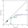 |
Fig. 8 Best-fit redshift values of the multiple image families compared with the spectroscopic, in blue, and photometric, in green, redshift values. The arrows indicate the unconstrained redshifts and the black line the relation zspec,phot = zbest fit. We use the spectroscopic redshift value measured from the Lyα blob for family 20. |
There is a well-known degeneracy between the mass of a lens (parametrised by σv) and the distance of a lensed source. Simplifying, as the source distance increases the lens mass has to decrease to match the same multiple image positions. From Table 4, the best-fitting redshift values of the model FZ2 are all systematically larger than those of the model F2. In Fig. 8, we compare the model-predicted redshifts (zbest fit) of all the 14 multiple image families with the spectroscopic (blue marks) and photometric (green) estimates from Jouvel et al. (2014), with 95% confidence level error bars. We choose the multiple image with the highest value of the odds parameter from the photo-z algorithm (see Sect. 3.3 of Jouvel et al. 2014) to associate only one photometric redshift value with each family. As expected, for the low-redshift families (zspec,phot< 2) the agreement between the model predictions and the measurements is very good. However, for families at higher redshifts the difference increases significantly and progressively, always leading to overestimate the redshift value. For families with zspec,phot> 4, redshifts are basically unconstrained, indicating that spectroscopic measurements for these sources become critical to avoid significant systematic uncertainties on the mass (and cosmological) parameters.
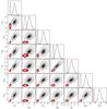 |
Fig. 9 Confidence regions for the redshifts values of the families with no spectroscopic confirmation. Red regions: the redshift values of the spectroscopically confirmed families are fixed. Grey regions: the redshift values of all families are left free. These correspond to models F2 and FZ2, respectively, in Table 4. The contours represent the 68%, 95.4%, and 99.7% confidence levels. |
In Fig. 9, we show the confidence regions, estimated from the MCMC analysis, of the best-fit redshifts for the model FZ2 (in grey) and F2 (in red). In the model FZ2 (all redshifts left free), the redshift values are all strongly correlated. This effect becomes larger, in absolute values, for the sources at higher redshifts. For the model F2, the confidence regions are much smaller and the correlation is much less pronounced. Moreover, the overlap of the confidence regions for the two models occur only at low redshifts and only in the 3σ area of the model FZ2, again indicating the bias introduced by the lack of spectroscopic information. The absence of information about the source redshifts results in a best-fitting model with a lower total mass for the cluster that is compensated by higher values for the source redshifts. The degeneracy between the total cluster mass and source redshifts explains the difference of ≈3% in the value of the effective velocity dispersion (σv), linked to the total cluster mass, of the models F1, F2 and FZ1, FZ2. For the model FZ2, we find a total mass projected within 250 kpc of  , a difference of approximately 4% when compared with F2. This shows that the measurements of the projected total mass are similar, despite the large redshift bias. On the contrary, since the best-fit redshift values are biased, we expect that quantities that depend directly on cosmological distances, such as Ξ in Eq. (9), will also be biased if spectroscopic redshifts are not available.
By leaving the redshift values of all families free, we increase the number of free parameters by 7 and 14 for family sample 1 and 2, respectively. Clearly, the larger number of free parameters reduces the value of the final Δrms (and consequently ), but biases the recovered parameters, principally the cosmological parameters. For the models WZ1 and WZ2, the best-fit cosmological parameters are Ωm = 1.0 and 0.6, and w =−1.4 and −1.3, respectively. These values are in disagreement with other established cosmological probes, showing that missing information on the background source redshifts makes cosmological constraints unreliable. In Sect. 4.3, however, we show that if one starts with a large sample of spectroscopically confirmed multiple image families, the addition of more secure families with no redshift information does not bias the estimates of the cosmological parameters.
4.3. Cosmological parameters
We focus here on the ability of the lensing model to constrain the cosmological parameters, by considering three different ΛCDM models: 1) a flat cosmological model with free Ωm and w (ID W); 2) a cosmological model with fixed w = −1, but allowing different curvature values, i.e. free Ωm and ΩΛ (ID L); and 3) a cosmological model with three parameters free, Ωm, ΩΛ, and w, (ID WL).
From Table 4, we find that the models with fixed cosmological parameters, F1 and F2, have larger Δrms values than those allowing some freedom in the background cosmological model, showing the leverage of the cosmological parameters on the multiple image positions. For instance, the reduced χ2 (/d.o.f.) decreases by ≈13% when we compare the model F1, including the spectroscopic confirmed families with fixed cosmology, with the models W1 and L1, where the value of the cosmological parameters are left free.
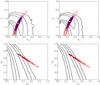 |
Fig. 10 Confidence levels (black lines) for the cosmological parameters of models W1 and W2 (Ωm + ΩΛ = 1, top panels) and L1 and L2 (w = −1, bottom panels). Left panels refer to strong lensing models using only spectroscopic families (L1, W1); models in the right panels include all families (L2, W2). Red lines: contours from Planck Data Release 2 data. Blue regions: combined constraints. The yellow circles indicate the maximum likelihood peak in this projection. |
In flat cosmological models, the 68% confidence levels for each parameter yield:  ,
,  and
and  ,
,  , for the models W1 and W2, respectively. By including family sample 2 (secure multiple images with unknown redshift), the statistical uncertainties on w is ≈20% smaller, but that on Ωm increases by ≈14%. This is caused by a tilt in the orientation of the degeneracy between these two parameters.
 |
Fig. 11 Confidence regions of the free parameters in the model considering all multiple image families and varying Ωm and w in a flat Universe (model W2). The contours represent the 68%, 95.4%, and 99.7% confidence levels. The lines indicate the maximum likelihood in the projection on each single parameter. Contours associated with constrained redshifts are omitted for clarity. |
It appears that the extra information included in the additional multiple image families leads to an improvement of the overall model, i.e. to smaller errors on the values of the lens mass distribution parameters and, consequently, of the cosmological parameters. The 68%, 95.4% and 99.7% confidence regions on the cosmological parameter plane are shown in the top panels of Fig. 10, for the models W1 and W2, respectively. The red contours indicate the confidence regions from the Planck satellite Data Release 2 (Planck Collaboration XIII 2015) and the blue regions show the combination with the likelihood from our strong lensing models. The agreement with the results from the CMB data, Ωm = 0.3089 ± 0.0062 and  , is very good (see Tables 4 and 5 in Planck Collaboration XIII 2015), and we emphasize the complementarity of the two different cosmological probes, making their combination in principle powerful.
In the bottom panels of Fig. 10, we show the confidence regions of the cosmological parameters for the models L1 and L2 (Ωm and ΩΛ free to vary and w = −1). Here, we find a clear degeneracy between the values of Ωm and ΩΛ, with the value of Ωm smaller than 0.7 at 99.7% confidence level and that of ΩΛ essentially unconstrained. Indeed, the results of the simulations performed by Gilmore & Natarajan (2009) showed that the values of the family ratios of Eq. (9), predicted by strong lensing models, are not very sensitive to changes in the value of the dark energy density parameter. For the models L1 and L2, we obtain  ,
,  and
and  ,
,  (68% confidence level), respectively.
In Fig. 11, we show for the model ID W2 the correlation between the parameters describing the total mass distribution of the lens and those related to the cosmological model. The histograms represent the probability density distributions of each free parameter, marginalized over all the other parameters. For visualization clarity, we do not show the redshifts of families 9, 13, 15, 16, 17, 20 and 21 in this figure, although they are also free parameters (see the model ID W2 in Table 5).
Figure 11 shows that the cosmological parameters are mainly degenerate with the σv parameter, which is associated with the mass of the cluster dark matter halo: Ωm and σv are positively correlated, while w and σv are strongly anti-correlated for low (w< −1) and high (>1500 km s-1) values, respectively. This result suggests that independent information about the total mass of a cluster, for example from galaxy dynamics (e.g. Biviano et al. 2013) or weak lensing (e.g. Umetsu et al. 2014), could further reduce the statistical uncertainties on recovered cosmological parameters. It remains important however to consider the impact of a number of systematics inherent in different methods of mass measurements.
In a previous work, Jullo et al. (2010) studied the same cosmological model using the galaxy cluster Abell 1689, a merging cluster located at z = 0.184. In that work, starting from a sample of 102 secure-spectroscopic multiple images, they considered a subsample of 28 multiple images from eight different families distributed in redshift between 1.50 and 3.05. Figure 2 of Jullo et al. (2010) shows the confidence regions in the Ωm-w plane, as obtained from their strong lensing analysis only and in combination with the results from CMB observations. Those results are qualitatively similar to our findings in Fig. 10. Small differences in the confidence regions of the two studies can be ascribed to the different parametrization of the total mass of the clusters (including a careful selection of the cluster members in our model), the configuration of the adopted multiple images, the source and cluster redshifts, and the treatment of the positional errors of multiple images.
To highlight the importance of having multiply lensed sources over a wide range of redshift when trying to constrain cosmological parameters, we also study specific models (W3 and L3 in Tables 4 and 5) in which we exclude the family at the highest redshift, z = 6.111 (ID 14). In these models, the final positional Δrms remains basically unchanged when compared to models W2 and L2, however, the constraints on the cosmological parameters become much weaker, as shown in Fig. 12 (model W3/L3: left/right panel). Although the confidence regions of the lens mass distribution parameters increase by less than ~10%, this high-redshift system has a significant leverage on the estimate of cosmological parameter. In this case, we find that the same confidence regions of Ωm and w increase by ≈50% from model W2 to W3 with Ωm now becoming largely unconstrained. Such a deterioration is even more evident for model L3, when compared to L2. This test highlights the importance of probing the widest possible redshift range with spectroscopic multiply lensed systems, when exploring cosmography with strong lensing techniques. Similar results from cluster-scale strong lensing simulations were presented by Golse et al. (2002), confirming the essential role played by spectroscopically confirmed systems over a large redshift range for accurate measurements of the values of the cosmological parameters. Finally, we mention that the models Wa1 and Wa2, which include a variation with redshift in the dark energy equation of state, can reproduce the observed multiple image positions only slightly better. This indicates very little sensitivity on the wa parameter in our current strong lensing models of RXC J2248.
5. Line-of-sight mass structure
To estimate the perturbing lensing effect of mass structures along the line of sight not included in the single-plane lens modelling of RXC J2248, we perform the following simplified tests with the Glee software, developed by A. Halkola and S. H. Suyu (Suyu & Halkola 2010; Suyu et al. 2012). We mimic the strong lensing geometry observed in RXC J2248 as close as possible, both in terms of angular positions and redshifts of the multiple images. In detail, we consider eight different sources lensed into 24 multiple images, distributed within a circle of ≈1′ in radius from the cluster centre and covering a redshift range between 1.0 and 6.1, thus following the observed configuration (see Table 1 and Fig. 1). The starting unperturbed positions of the 24 images are perfectly fitted, i.e. with a null rms offset, by only one PIEMD mass profile, with parameter values very close to those shown in Table 4 and within a fixed cosmological model with Ωm = 0.3, ΩΛ = 0.7, w = −1.0, and H0 = 70 km s-1 Mpc-1. Then, we simulate plausible lens galaxies along the line of sight, modelled as dPIE mass distributions with vanishing ellipticity and core radius, introduce their mass components in the lensing model, and calculate the perturbed multiple image positions. We use these new positions as observables to optimize the parameters of the PIEMD mass profile, neglecting the contribution of the secondary line-of-sight deflectors. This should represent the typical lensing modelling situation in which the parameters describing the total mass distribution of a galaxy cluster, acting as a primary deflector on background sources, are measured by fitting the positions of a set of multiple images in the single-plane lens approximation, i.e. ignoring the effect of possible mass structures along the line of sight.
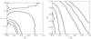 |
Fig. 12 Confidence regions on the cosmological parameter planes when all multiple image systems are used with the exception of the highest redshift (z = 6.111) family (left: model W3; right: model L3). |
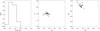 |
Fig. 13 Left panel: probability distribution function, obtained from the set of 20 simulations, of the Δrms offset between the perturbed and best-fitting model-predicted positions of the 24 multiple images. The predicted positions are determined by optimizing the parameters of the total mass distribution of the main lens not including the mass perturbers along the line-of-sight. Middle and right panels: best-fitting values of the parameters Ωm, ΩΛ and w from the set of 20 simulations. These values are determined by optimizing the parameters of the total mass distribution of the main lens and of the cosmological model not including in the mass perturbers along the line-of-sight. |
Initially, we add a single dPIE perturber to the PIEMD mass component. We fix the values of its distance from the cluster centre and effective velocity dispersion to 60 arcsec and 200 km s-1, respectively. We then vary the redshift value of the dPIE component from 0.05 to 0.65 with a constant step of 0.1. To obtain non-negligible perturbing lensing effects, we purposely simulate such a massive galaxy, close in projection to the Einstein radius of the cluster for the source at the highest redshift. The optimized PIEMD mass models (without varying the cosmological parameters) can reproduce the perturbed multiple-image positions with Δrms values that range from 0.3 to 0.1 arcsec, decreasing systematically with the redshift of the perturber. This simple test confirms the results of previous studies (e.g. McCully et al. 2014) which have shown that statistically, at fixed total mass values, mass concentrations in the foreground of a main deflector affect the lensed positions of the multiple images more significantly than mass concentrations in the background. We remark that massive foreground or member galaxies are rarely omitted in the lensing model of a galaxy cluster because these galaxies are usually very luminous and easily identified as important lensing components (e.g. see Sect. 3.4 in Grillo et al. 2015b). Therefore, rms values of 0.3 arcsec or larger associated with only one massive and neglected line-of-sight structure are not very likely in detailed strong lensing models.
Next, we consider a set of 20 more realistic simulations, each of which containing ten different dPIE mass components. The position and mass parameters of these components are extracted from uniform distributions in the following ranges: mass centres, in angular coordinates x and y from the cluster centre, between −60 and 60 arcsec, redshift values between 0 and 0.8, and effective velocity dispersion values between 25 and 175 km s-1. As above, for each simulation we optimize the PIEMD mass parameters, not modelling the perturbers and not changing the cosmological parameters, and estimate the rms offset Δ between the perturbed and model-predicted positions of the multiple images. The results are summarized in the first panel of Fig. 13. The probability distribution function of Δ has mean and standard deviation values of 0.3 and 0.1 arcsec, respectively. An offset of approximately 0.3 arcsec in the reproduction of the observed multiple-image positions has been found in our best-fitting strong lensing models of RXC J2248 (see Sect. 4), MACS J0416 (e.g., see Sect. 3.5.1 in Grillo et al. 2015b) and MACS J1149 (e.g. see Sect. 3.4 in Grillo et al. 2015a), which have been obtained in the single-plane lens approximation, as in these simulations. Moreover, we investigate the systematic uncertainty on the values of the cosmological parameters introduced by neglecting the mass structure along the line of sight. To do so, we add the values of Ωm, ΩΛ, and w to the PIEMD mass parameters in the modelling optimization performed on the same sample of 20 sets of perturbed multiple-image positions. Allowing three additional (cosmological) parameters to vary leads to average rms values that are approximately 10% smaller than the previous values. We show the best-fitting values of Ωm, ΩΛ and w in the second and third panels of Fig. 13, and estimate the median with standard deviation values of 0.3 ± 0.1, 0.8 ± 0.1, and −1.0 ± 0.1, respectively. The comparison of Figs. 10 and 13 suggests that the total (statistical+systematic) degeneracy between the values of Ωm and w is likely not driven by the systematic effect of the unmodelled line-of-sight mass structure. The results of Fig. 11 (in particular the σv-w panel) and Fig. 13 indicate that additional information about the total mass is needed from different diagnostics to reduce the uncertainties on the values of Ωm and w.
We caution that we obtained the previous results through simplified total mass models of a galaxy cluster that does not contain cluster members. We have purposely chosen this approach to reduce the degeneracies among the parameters describing the relative mass contributions of the cluster and cluster members and thus facilitate the interpretation of the test outcome. We postpone to a future work a more thorough analysis including the cluster members. The spectroscopic CLASH-VLT programme and additional VLT/MUSE follow-up campaigns (e.g. in RXC 2248, see Karman et al. 2015; and in MACS J1149, see Treu et al. 2016 and Grillo et al. 2015a) have identified the mass structures along the line of sight that should be incorporated in the ultimate strong lensing models of galaxy clusters. Unfortunately, at the time when this analysis was performed none of the lensing codes available could fully model line-of-sight mass structures and carefully quantify the impact of this effect on the reconstructed values of the cluster mass and cosmological parameters. The Glee software has recently been updated to include multiple plane lensing, which will be presented in future works.
6. Conclusions
In this paper, we perform a comprehensive strong lensing analysis of the galaxy cluster RXC J2248 based on HST imaging and new extensive VLT spectroscopy with the VIMOS and MUSE instruments. We also find an extended Lyα emitter at redshift 3.118, which is one of the first cases identified of a multiply lensed “Lyα blob”. We consider 22 lensing models with different mass model parametrization, samples of multiple images, and assumptions on the free parameters. We show that RXC J2248 is a massive cluster, which is particularly suitable for constraining the background geometry of the Universe with strong lensing modelling, because of its unique combination of a regular shape, a large number of multiple images spanning a wide redshift range, and a relatively modest presence of an intervening large-scale structure, as revealed by our spectroscopic survey. We show that the accuracy with which we reproduce the observed positions of the multiple images ( ) is such that the perturbing effect of mass structures along the line of sight needs to be taken properly into account for further improvements. Future work will also need to focus on reducing systematics in the total mass-light scaling relation of the sub-halo population and this can be achieved by using measured velocity dispersions of the BCG and other bright cluster galaxies (e.g. Monna et al. 2015). The main results of this study can be summarized as follows:
-
1.
We reconstruct the observed positions of 38 multiple imagesfrom 14 different sources in the redshift range1.035−6.111 with an accuracy of
in our reference model F2 (see Table 4). -
2.
By testing different lensing models we show that the total mass density distribution in the centre (R ≲ 300 kpc) of RXC J2248 is better represented by a PIEMD profile rather than a NFW. This is basically because of the existence of a significant core in the inner regions.
-
3.
Owing to the wide redshift range of secure multiply lensed sources and the regular mass distribution of RXC J2248, we are able to significantly alleviate degeneracies when simultaneously fitting the background geometry of the Universe and the total mass distribution of the lens in our strong lensing analyses. We thus find in the strong lensing analyses only that
 and
and  for a flat ΛCDM model and
  and
and  for a Universe with free curvature but w = −1.
 -
4.
We show that spectroscopic information is critical for a high-precision strong lensing model. The lack of spectroscopic measurements of the multiply lensed sources or the use of photometric redshifts can bias the results on the values of the cosmological parameters, although the impact on the estimate of the total mass of the lens is not very significant. Moreover, a wide redshift range of multiply lensed sources is also critical to increase the leverage on cosmology.
-
5.
Simple simulations, aimed at estimating the impact of line-of-sight perturbers on the lens modelling, show that this effect can introduce a scatter of (0.3 ± 0.1)″ in the multiple image positions, which is of the same order of the statistical errors achieved by our models.
We anticipate that repeating this experiment on other CLASH-VLT clusters, with similar high-quality samples of multiple images, leads instead to very loose constraints on cosmological parameters in cases where the spectroscopic campaign reveals significant large-scale structures along the line of sight. This suggests that a more sophisticated treatment of the oberved line-of-sight effects is needed in the lensing models to overcome this fundamental limit of lensing techniques. This will be the subject of future papers.
Acknowledgments
We thank the ESO User Support group for excellent support on the implementation of the Large Programme 186.A-0798. The CLASH Multi-Cycle Treasury Program is based on observations made with the NASA/ESA Hubble Space Telescope. This work made use of MUSE data taken under programme ID 60.A-9345(A), during the science verification period. The authors thank the referee Marceau Limousin for useful comments on this paper. G.B.C. is supported by the CAPES-ICRANET programme through the grant BEX 13946/13-7. C.G. and E.M. acknowledge support by VILLUM FONDEN Young Investigator Programme through grant No. 10123. This work made use of the CHE cluster, managed and funded by ICRA/CBPF/MCTI, with financial support from FINEP (grant 01.07.0515.00 from CT-INFRA - 01/2006) and FAPERJ (grants E-26/171.206/2006 and E-26/110.516/2012). We acknowledge support from PRIN-INAF 2014 1.05.01.94.02 (PI M. Nonino). P.R. acknowledges the hospitality and support of the visitor programme of the DFG cluster of excellence “Origin and Structure of the Universe”. A.Z. is supported by NASA through Hubble Fellowship grant #HST-HF2-51334.001-A awarded by STScI.
References
- Abell, G. O., Corwin, Jr., H. G., & Olowin, R. P. 1989, ApJS, 70, 1 [NASA ADS] [CrossRef] [EDP Sciences] [Google Scholar]
- Arrigoni Battaia, F., Hennawi, J. F., Prochaska, J. X., & Cantalupo, S. 2015, ApJ, 809, 163 [NASA ADS] [CrossRef] [Google Scholar]
- Bacon, R., Accardo, M., Adjali, L., et al. 2010, in SPIE Conf. Ser., 7735, 8 [Google Scholar]
- Balestra, I., Vanzella, E., Rosati, P., et al. 2013, A&A, 559, L9 [NASA ADS] [CrossRef] [EDP Sciences] [Google Scholar]
- Bertin, E., & Arnouts, S. 1996, A&AS, 117, 393 [NASA ADS] [CrossRef] [EDP Sciences] [Google Scholar]
- Biviano, A., Rosati, P., Balestra, I., et al. 2013, A&A, 558, A1 [NASA ADS] [CrossRef] [EDP Sciences] [Google Scholar]
- Boone, F., Clément, B., Richard, J., et al. 2013, A&A, 559, L1 [NASA ADS] [CrossRef] [EDP Sciences] [Google Scholar]
- Bouwens, R. J., Illingworth, G. D., Oesch, P. A., et al. 2011, ApJ, 737, 90 [NASA ADS] [CrossRef] [Google Scholar]
- Caminha, G. B., Karman, W., Rosati, P., et al. 2015, A&A, submitted [arXiv:1512.05655] [Google Scholar]
- Collett, T. E., & Auger, M. W. 2014, MNRAS, 443, 969 [NASA ADS] [CrossRef] [Google Scholar]
- Efstathiou, G., Moody, S., Peacock, J. A., et al. 2002, MNRAS, 330, L29 [NASA ADS] [CrossRef] [Google Scholar]
- Eisenstein, D. J., Zehavi, I., Hogg, D. W., et al. 2005, ApJ, 633, 560 [NASA ADS] [CrossRef] [Google Scholar]
- Elíasdóttir, Á., Limousin, M., Richard, J., et al. 2007, ArXiv e-prints [arXiv:0710.5636] [Google Scholar]
- Francis, P. J., Williger, G. M., Collins, N. R., et al. 2001, ApJ, 554, 1001 [NASA ADS] [CrossRef] [Google Scholar]
- Fynbo, J. U., Møller, P., & Warren, S. J. 1999, MNRAS, 305, 849 [NASA ADS] [CrossRef] [Google Scholar]
- Gilmore, J., & Natarajan, P. 2009, MNRAS, 396, 354 [NASA ADS] [CrossRef] [Google Scholar]
- Gilmour, R., Best, P., & Almaini, O. 2009, MNRAS, 392, 1509 [NASA ADS] [CrossRef] [Google Scholar]
- Golse, G., & Kneib, J.-P. 2002, A&A, 390, 821 [NASA ADS] [CrossRef] [EDP Sciences] [Google Scholar]
- Golse, G., Kneib, J.-P., & Soucail, G. 2002, A&A, 387, 788 [NASA ADS] [CrossRef] [EDP Sciences] [Google Scholar]
- Gómez, P. L., Valkonen, L. E., Romer, A. K., et al. 2012, AJ, 144, 79 [NASA ADS] [CrossRef] [Google Scholar]
- Grillo, C., Lombardi, M., & Bertin, G. 2008, A&A, 477, 397 [NASA ADS] [CrossRef] [EDP Sciences] [Google Scholar]
- Grillo, C., Karman, W., Suyu, S. H., et al. 2015a, ArXiv e-prints [arXiv:1511.04093] [Google Scholar]
- Grillo, C., Suyu, S. H., Rosati, P., et al. 2015b, ApJ, 800, 38 [NASA ADS] [CrossRef] [Google Scholar]
- Gruen, D., Brimioulle, F., Seitz, S., et al. 2013, MNRAS, 432, 1455 [NASA ADS] [CrossRef] [Google Scholar]
- Halkola, A., Hildebrandt, H., Schrabback, T., et al. 2008, A&A, 481, 65 [NASA ADS] [CrossRef] [EDP Sciences] [Google Scholar]
- Halkola, A., Seitz, S., & Pannella, M. 2006, MNRAS, 372, 1425 [NASA ADS] [CrossRef] [Google Scholar]
- Host, O. 2012, MNRAS, 420, L18 [NASA ADS] [CrossRef] [Google Scholar]
- Johnson, T. L., Sharon, K., Bayliss, M. B., et al. 2014, ApJ, 797, 48 [NASA ADS] [CrossRef] [Google Scholar]
- Jouvel, S., Host, O., Lahav, O., et al. 2014, A&A, 562, A86 [NASA ADS] [CrossRef] [EDP Sciences] [Google Scholar]
- Jullo, E., Kneib, J.-P., Limousin, M., et al. 2007, New J. Phys., 9, 447 [Google Scholar]
- Jullo, E., Natarajan, P., Kneib, J.-P., et al. 2010, Science, 329, 924 [NASA ADS] [CrossRef] [PubMed] [Google Scholar]
- Karman, W., Caputi, K. I., Grillo, C., et al. 2015, A&A, 574, A11 [NASA ADS] [CrossRef] [EDP Sciences] [Google Scholar]
- Kassiola, A., & Kovner, I. 1993, ApJ, 417, 450 [NASA ADS] [CrossRef] [Google Scholar]
- Keeton, C. R. 2001, ArXiv e-prints [arXiv:astro-ph/0102340] [Google Scholar]
- Kneib, J.-P. 2002, in The Shapes of Galaxies and their Dark Halos, ed. P. Natarajan, 50 [Google Scholar]
- Kneib, J.-P., Ellis, R. S., Smail, I., Couch, W. J., & Sharples, R. M. 1996, ApJ, 471, 643 [NASA ADS] [CrossRef] [Google Scholar]
- Koekemoer, A. M., Faber, S. M., Ferguson, H. C., et al. 2011, ApJS, 197, 36 [NASA ADS] [CrossRef] [Google Scholar]
- Komatsu, E., Smith, K. M., Dunkley, J., et al. 2011, ApJS, 192, 18 [NASA ADS] [CrossRef] [Google Scholar]
- Laporte, C. F. P., & White, S. D. M. 2015, MNRAS, 451, 1177 [NASA ADS] [CrossRef] [Google Scholar]
- Le Fèvre, O., Saisse, M., Mancini, D., et al. 2003, in Instrument Design and Performance for Optical/Infrared Ground-based Telescopes, eds. M. Iye, & A. F. M. Moorwood, SPIE Conf. Ser., 4841, 1670 [Google Scholar]
- Magaña, J., Motta, V., Cárdenas, V. H., Verdugo, T., & Jullo, E. 2015, ApJ, 813, 69 [NASA ADS] [CrossRef] [Google Scholar]
- Maughan, B. J., Jones, C., Forman, W., & Van Speybroeck, L. 2008, ApJS, 174, 117 [NASA ADS] [CrossRef] [Google Scholar]
- McCully, C., Keeton, C. R., Wong, K. C., & Zabludoff, A. I. 2014, MNRAS, 443, 3631 [NASA ADS] [CrossRef] [Google Scholar]
- Melchior, P., Suchyta, E., Huff, E., et al. 2015, MNRAS, 449, 2219 [NASA ADS] [CrossRef] [Google Scholar]
- Merten, J., Meneghetti, M., Postman, M., et al. 2015, ApJ, 806, 4 [NASA ADS] [CrossRef] [Google Scholar]
- Monna, A., Seitz, S., Greisel, N., et al. 2014, MNRAS, 438, 1417 [NASA ADS] [CrossRef] [Google Scholar]
- Monna, A., Seitz, S., Zitrin, A., et al. 2015, MNRAS, 447, 1224 [NASA ADS] [CrossRef] [Google Scholar]
- Navarro, J. F., Frenk, C. S., & White, S. D. M. 1996, ApJ, 462, 563 [NASA ADS] [CrossRef] [Google Scholar]
- Navarro, J. F., Frenk, C. S., & White, S. D. M. 1997, ApJ, 490, 493 [NASA ADS] [CrossRef] [Google Scholar]
- Nilsson, K. K., Fynbo, J. P. U., Møller, P., Sommer-Larsen, J., & Ledoux, C. 2006, A&A, 452, L23 [NASA ADS] [CrossRef] [EDP Sciences] [Google Scholar]
- Perlmutter, S., Aldering, G., Goldhaber, G., et al. 1999, ApJ, 517, 565 [NASA ADS] [CrossRef] [Google Scholar]
- Planck Collaboration XVI. 2014, A&A, 571, A16 [NASA ADS] [CrossRef] [EDP Sciences] [Google Scholar]
- Planck Collaboration XIII. 2015, A&A, submitted [arXiv:1502.01589] [Google Scholar]
- Postman, M., Coe, D., Benítez, N., et al. 2012a, ApJS, 199, 25 [NASA ADS] [CrossRef] [Google Scholar]
- Postman, M., Lauer, T. R., Donahue, M., et al. 2012b, ApJ, 756, 159 [Google Scholar]
- Richard, J., Jauzac, M., Limousin, M., et al. 2014, MNRAS, 444, 268 [NASA ADS] [CrossRef] [Google Scholar]
- Riess, A. G., Filippenko, A. V., Challis, P., et al. 1998, AJ, 116, 1009 [NASA ADS] [CrossRef] [Google Scholar]
- Rosati, P., Balestra, I., Grillo, C., et al. 2014, The Messenger, 158, 48 [NASA ADS] [Google Scholar]
- Rousseeuw, P. J. 1984, J. Am. Statistical Association, 79, 871 [Google Scholar]
- Schneider, P., Ehlers, J., & Falco, E. E. 1992, Gravitational Lenses (Springer-Verlag) [Google Scholar]
- Schwab, J., Bolton, A. S., & Rappaport, S. A. 2010, ApJ, 708, 750 [Google Scholar]
- Soucail, G., Kneib, J.-P., & Golse, G. 2004, A&A, 417, L33 [NASA ADS] [CrossRef] [EDP Sciences] [Google Scholar]
- Steidel, C. C., Adelberger, K. L., Shapley, A. E., et al. 2000, ApJ, 532, 170 [Google Scholar]
- Suyu, S. H., & Halkola, A. 2010, A&A, 524, A94 [NASA ADS] [CrossRef] [EDP Sciences] [Google Scholar]
- Suyu, S. H., Marshall, P. J., Auger, M. W., et al. 2010, ApJ, 711, 201 [NASA ADS] [CrossRef] [Google Scholar]
- Suyu, S. H., Hensel, S. W., McKean, J. P., et al. 2012, ApJ, 750, 10 [NASA ADS] [CrossRef] [Google Scholar]
- Suyu, S. H., Auger, M. W., Hilbert, S., et al. 2013, ApJ, 766, 70 [NASA ADS] [CrossRef] [Google Scholar]
- Tollet, E., Macciò, A. V., Dutton, A. A., et al. 2016, MNRAS, 456, 3542 [NASA ADS] [CrossRef] [Google Scholar]
- Treu, T., Schmidt, K. B., Brammer, G. B., et al. 2015, ApJ, 812, 114 [NASA ADS] [CrossRef] [Google Scholar]
- Treu, T., Brammer, G., Diego, J. M., et al. 2016, ApJ, 817, 60 [NASA ADS] [CrossRef] [Google Scholar]
- Umetsu, K., Medezinski, E., Nonino, M., et al. 2014, ApJ, 795, 163 [NASA ADS] [CrossRef] [Google Scholar]
- Zitrin, A., Fabris, A., Merten, J., et al. 2015, ApJ, 801, 44 [NASA ADS] [CrossRef] [Google Scholar]
All Tables
Log of VIMOS observations of the Frontier Fields cluster RXC J2248, taken as part of the CLASH-VLT spectroscopic campaign.
All Figures
|
Fig. 1 Colour composite image of RXC J2248 obtained using the 16 HST/ACS and WFC3 filters. Spectroscopically confirmed multiple images are indicated in red; multiple images with no spectroscopic redshift in magenta. White circles indicate sources close to a cluster member, or possibly lensed by line-of-sight structures, or with not secure counter images. These last images are not used in the lens model. More information is provided in Table 1. The blue circle shows the position of the BCG. The multiple image ID 14e is only used in the model F1-5th; see Table 4. |
| In the text | |
|
Fig. 2 Colour composite image of RXC J2248 overlaid with the Chandra X-ray contours in white (Gómez et al. 2012). Red circles indicate the selected cluster members (see Sect. 3.1.2). The magenta circle shows the second brightest cluster member, used as the reference for the normalization of the mass-to-light ratio of the cluster members, i.e. L0 in Eq. (3). |
| In the text | |
|
Fig. 3 VLT/VIMOS spectra of the multiple image systems. Left panels: HST cutouts, 10′′ across with the position of the VIMOS 1′′-wide slits and the image ID from Table 1. One- and two-dimensional spectra are shown on the right with measured redshifts and quality flags, including typical emission and absorption lines. |
| In the text | |
|
Fig. 3 continued. |
| In the text | |
|
Fig. 3 continued. |
| In the text | |
|
Fig. 4 MUSE 1D spectra of the multiple images 8a and 8b. The vertical lines indicate the CIII] doublet emission wavelengths of a source at redshift 1.837. The small panels show the circles with 1″ (top) and |
| In the text | |
|
Fig. 5 MUSE 1D spectra of the multiple images 20a and 20b. The vertical line indicates the Lyα emission wavelength of a source at redshift 3.118. The small panels show the circles with 1″ radius used to extract the two spectra. The flux is rescaled by a factor of 10-18 erg / s / cm2/Å. |
| In the text | |
|
Fig. 6 CLASH/HST colour cutouts (4″ wide) of all multiple images used in the reference model F2. Red circles ( |
| In the text | |
|
Fig. 6 continued. |
| In the text | |
|
Fig. 7 Distribution of the displacement values of the multiple images (absolute values of the observed minus the reconstructed positions, see Eq. (6)) obtained from our reference model F2 (solid blue line) and in previous works by Monna et al. (2014; green dashed) and Johnson et al. (2014; red long dashed), for the cluster RXC J2248. |
| In the text | |
|
Fig. 8 Best-fit redshift values of the multiple image families compared with the spectroscopic, in blue, and photometric, in green, redshift values. The arrows indicate the unconstrained redshifts and the black line the relation zspec,phot = zbest fit. We use the spectroscopic redshift value measured from the Lyα blob for family 20. |
| In the text | |
|
Fig. 9 Confidence regions for the redshifts values of the families with no spectroscopic confirmation. Red regions: the redshift values of the spectroscopically confirmed families are fixed. Grey regions: the redshift values of all families are left free. These correspond to models F2 and FZ2, respectively, in Table 4. The contours represent the 68%, 95.4%, and 99.7% confidence levels. |
| In the text | |
|
Fig. 10 Confidence levels (black lines) for the cosmological parameters of models W1 and W2 (Ωm + ΩΛ = 1, top panels) and L1 and L2 (w = −1, bottom panels). Left panels refer to strong lensing models using only spectroscopic families (L1, W1); models in the right panels include all families (L2, W2). Red lines: contours from Planck Data Release 2 data. Blue regions: combined constraints. The yellow circles indicate the maximum likelihood peak in this projection. |
| In the text | |
|
Fig. 11 Confidence regions of the free parameters in the model considering all multiple image families and varying Ωm and w in a flat Universe (model W2). The contours represent the 68%, 95.4%, and 99.7% confidence levels. The lines indicate the maximum likelihood in the projection on each single parameter. Contours associated with constrained redshifts are omitted for clarity. |
| In the text | |
|
Fig. 12 Confidence regions on the cosmological parameter planes when all multiple image systems are used with the exception of the highest redshift (z = 6.111) family (left: model W3; right: model L3). |
| In the text | |
|
Fig. 13 Left panel: probability distribution function, obtained from the set of 20 simulations, of the Δrms offset between the perturbed and best-fitting model-predicted positions of the 24 multiple images. The predicted positions are determined by optimizing the parameters of the total mass distribution of the main lens not including the mass perturbers along the line-of-sight. Middle and right panels: best-fitting values of the parameters Ωm, ΩΛ and w from the set of 20 simulations. These values are determined by optimizing the parameters of the total mass distribution of the main lens and of the cosmological model not including in the mass perturbers along the line-of-sight. |
| In the text | |
Current usage metrics show cumulative count of Article Views (full-text article views including HTML views, PDF and ePub downloads, according to the available data) and Abstracts Views on Vision4Press platform.
Data correspond to usage on the plateform after 2015. The current usage metrics is available 48-96 hours after online publication and is updated daily on week days.
Initial download of the metrics may take a while.