| Issue |
A&A
Volume 584, December 2015
|
|
|---|---|---|
| Article Number | A70 | |
| Number of page(s) | 15 | |
| Section | Interstellar and circumstellar matter | |
| DOI | https://doi.org/10.1051/0004-6361/201526466 | |
| Published online | 24 November 2015 | |
Spectroscopically resolved far-IR observations of the massive star-forming region G5.89–0.39
1 Max-Planck-Institut für Radioastronomie, Auf dem Hügel 69, 53121 Bonn, Germany
e-mail: sleurini@mpifr.de
2 LERMA, Observatoire de Paris, École Normale Supérieure, PSL Research University, CNRS, UMR 8112, 75014 Paris, France
3 Sorbonne Universités, UPMC Univ. Paris 6, UMR 8112, LERMA, 75005 Paris, France
4 Deutsches Zentrum für Luft-und Raumfahrt (DLR), Institute of Optical Sensor Systems, Rutherfordstrasse 2, 12489 Berlin, Germany
5 Humboldt-Universität zu Berlin, Department of Physics, Newtonstr. 15, 12489 Berlin, Germany
6 Kölner Observatorium für Submm Astronomie (KOSMA), I. Physikalisches Institut, Universität zu Köln, Zülpicher Str. 77, 50937 Cologne, Germany
Received: 4 May 2015
Accepted: 26 August 2015
Context. The fine-structure line of atomic oxygen at 63 μm ([OI]63μm) is an important diagnostic tool in different fields of astrophysics: it is for example predicted to be the main coolant in several environments of star-forming regions (SFRs). However, our knowledge of this line relies on observations with low spectral resolution, and the real contribution of each component (photon-dominated region, jet) in the complex environment of SFRs to its total flux is poorly understood.
Aims. We investigate the contribution of jet and photon-dominated region emission, and of absorption to the [OI]63μm line towards the hot gas around the ultra-compact Hii region G5.89–0.39 and study the far-IR line luminosity of the source in different velocity regimes through spectroscopically resolved spectra of atomic oxygen, [CII], CO, OH, and H2O.
Methods. We mapped G5.89–0.39 in [OI]63μm and in CO(16–15) with the GREAT receiver onboard SOFIA. We also observed the central position of the source in the ground-state OH 2Π3/2 J = 5/2 → J = 3/2 triplet and in the excited OH 2Π1/2 J = 3/2 → J = 1/2 triplets with SOFIA. These data were complemented with APEX CO(6–5) and CO(7–6) maps and with Herschel/HIFI maps and single-pointing observations in lines of [CII], H2O, and HF.
Results. The [OI] spectra in G5.89–0.39 are severely contaminated by absorptions from the source envelope and from different clouds along the line of sight. Emission is detected only at high velocities, and it is clearly associated with the compact north-south outflows traced by extremely high-velocity emission in low-J CO lines. The mass-loss rate and the energetics of the jet system derived from the [OI]63μm line agree well with previous estimates from CO, thus suggesting that the molecular outflows in G5.89–0.39 are driven by the jet system seen in [OI]. The far-IR line luminosity of G5.89–0.39 is dominated by [OI] at high-velocities; the second coolant in this velocity regime is CO, while [CII], OH and H2O are minor contributors to the total cooling in the outflowing gas. Finally, we derive abundances of different molecules in the outflow: water has low abundances relative to H2 of 10-8−10-6, and OH of 10-8. Interestingly, we find an abundance of HF to H2 of 10-8, comparable with measurements in diffuse gas.
Conclusions. Our study shows the importance of spectroscopically resolved observations of the [OI]63μm line for using this transition as diagnostic of star-forming regions. While this was not possible until now, the GREAT receiver onboard SOFIA has recently opened the possibility of detailed studies of the [OI]63μm line to investigate the potential of the transition for probing different environments.
Key words: stars: formation / stars: kinematics and dynamics / ISM: jets and outflows / ISM: individual objects: G5.89-0.39 / shock waves / acceleration of particles
© ESO, 2015
1. Introduction
The fine-structure line of atomic oxygen at 63 μm ([OI]63μm) has an important diagnostic value in several fields of astrophysics. It is expected to be one of the main coolants in jets from young stellar objects (YSOs; e.g., Hollenbach & McKee 1989) and therefore to be a direct tracer of mass-loss rates (Hollenbach 1985). The [OI]63μm transition is also predicted to be a major coolant in photon-dominated regions (PDRs; Tielens & Hollenbach 1985; Sternberg & Dalgarno 1995), where, together with the [CII] fine structure line at 158 μm, it can be used as diagnostic tool of the physical conditions (e.g., Tielens & Hollenbach 1985). Observations show that [OI]63μm is an important PDR cooling line in external galaxies (e.g., Malhotra et al. 2001; Dale et al. 2004; Coppin et al. 2012). Since it suffers less from extinction than shorter wavelength lines, the [OI]63μm line might also be a powerful tracer of star-formation rates in galaxies even at high red-shifts (e.g., De Looze et al. 2014). Studies of [OI]63μm exist, mostly in galactic star-forming regions (Poglitsch et al. 1996; Kraemer et al. 1998; Giannini et al. 2001; Nisini et al. 2002; Ceccarelli et al. 1997; Malhotra et al. 2001). However, the diagnostic capabilities of this transition have not been fully exploited until now due to the poor angular and spectral resolutions and the poor sensitivity of previous instruments (ISO and KAO). This situation has recently improved with the PACS instrument onboard Herschel, which allowed observing atomic oxygen at 63 μm with an angular resolution of 9.̋4 and low spectral resolution (e.g., Podio et al. 2012; Goicoechea et al. 2013; Nisini et al. 2015).
 |
Fig. 1 Overview (left) of the large scale east-west outflow and zoom (right) in the inner region powering the extremely high-velocity molecular outflows in CO(2–1) imaged with SMA from Su et al. (2012). The figures are adapted from Hunter et al. (2008) and Su et al. (2012). In the left panel, contours show the large-scale CO(1–0) outflow from Watson et al. (2007), pentagons are class I methanol masers (Kurtz et al. 2004), while crosses indicate the submillimetre-millimetre dust sources (Hunter et al. 2008). The dashed and dotted lines show the axes of the outflows detected at high velocities by Su et al. (2012). In the right panel, the red box delineates the region mapped in [OI]63μm; the red dots are the centres of the [OI]63μm raster map. The overlaid colour scale represents the cm free–free emission (Tang et al. 2009), filled triangles are the H2 knots, open circles are class I methanol maser positions, and open squares are positions of water masers (Hofner & Churchwell 1996). The crosses mark the position of the submillimetre-millimetre dust components. The ellipse shows the beam of the SMA observations from Su et al. (2012). |
However, previous observations and modelling of the [OI]63μm line luminosity (e.g., Poglitsch et al. 1996; Liseau et al. 2006; Gerin et al. 2015; Rosenberg et al. 2015) suggested that spectrally unresolved observations of the 63 μm [OI] line can be difficult to interpret not only because several components (jet, PDRs) can contribute to its emission, but also because absorption from foreground clouds and self-absorption can contaminate the profile, thus undermining the diagnostic power of [OI]63μm based on observations with poor spectral resolution. The GREAT1 instrument onboard SOFIA finally provides the astronomical community with the high spectral and angular resolution that is needed to investigate the profile of the 63 μm line and study its spatial distribution on a 6.̋6 angular size scale.
We present here SOFIA observations of the massive star-forming region G5.89–0.39 in [OI]63μm aimed at resolving the distribution of atomic oxygen in the source and studying its line profile. The observations are complemented by spectroscopically resolved data of other main coolants (H2O, OH, CO, [CII]) from SOFIA/GREAT, the High Frequency Heterodyne Instrument of the Far infrared (HIFI) onboard Herschel, and the Atacama Pathfinder Experiment (APEX) 12 m telescope to study the contribution of each major contributor to the total far-IR luminosity as a function of velocity. G5.89–0.39 is an ideal target on which to demonstrate the complexity that the [OI]63μm emission can attain. Its distance ambiguity was recently solved through parallax measurements by Motogi et al. (2011), who located it at 1.28 kpc. It harbours a shell-like ultra-compact Hii region powered by a young O-type star (the so-called Feldt’s star, Feldt et al. 2003), which is visible in the near-IR. The region shows prominent outflow activity: at least three outflows are associated with a hot dusty and molecular cocoon surrounding the ultra-compact Hii region (Hunter et al. 2008; Su et al. 2009). The most prominent is a gigantic outflow aligned along the east-west direction that was discovered in CO emission by Harvey & Forveille (1988). The other two compact outflows were detected with the Submillimter Array (SMA) by Hunter et al. (2008) and Su et al. (2012) and are associated with extremely high-velocity material. These two flows are aligned along the north-south and north/west-south/east directions and are associated with H2 knots (Puga et al. 2006). The region is illustrated in Fig. 1, where the main components of the source are labelled.
This paper is organised as follows: in Sect. 2 we provide the technical information related to the observations and the calibration of the data performed with SOFIA and present the retrieved Herschel and APEX archival data. In Sect. 3 we discuss the [OI]63μm profile and its morphology and compare the spectra of the different atomic and molecular features toward the central position. In Sect. 4 the column densities and relative abundances of different species are derived in two different velocity ranges from absorption and emission features. In Sect. 5 we derive the mass-loss rate and other parameters describing the energetics of the outflow system from [OI]63μm. Finally, the total far-IR line luminosity of the source is derived in Sect. 6 in different velocity ranges and over the total line profile.
Summary of the observations.
2. Observations and data calibration
2.1. SOFIA observations
The SOFIA observations we present here were carried out with the GREAT (Heyminck et al. 2012) receiver during observatory cycles 1 and 2. The ground-state transition of [OI] at 4744.77749 GHz was observed on 2014 May 17 (observatory cycle 2) with the H channel of GREAT using a novel waveguide hot electron bolometer heterodyne mixer with state-of-the-art sensitivity (Büchel et al. 2015). The tuning of its local oscillator, a quantum-cascade laser (Hübers et al. 2013), is fixed to the rest frequency of this line. The Doppler correction was then applied off-line to the raw data. The atmospheric opacity at this frequency is due to the wing of a nearby water vapour feature and to the quasi-continuous collision-induced absorption by N2 and O2. At the flight altitude of 13 360 m, the bulk of these contributions is left below, and the residual water vapour along the sightline is lower than 10 μm. The telluric [OI] line, originating from the mesosphere, contributes a significant but narrow absorption feature. We describe in the next paragraph how we corrected for this. The resulting bandpass-averaged zenith opacity has a median value of 0.11; the double-sideband system temperature was 2435 K. The CO J = 16 → 15 line at 1841.345 GHz was observed in parallel with the L2 channel of GREAT with a system temperature (in the relevant part of the noise bandpass) of 2012 K (single sideband) at a zenith opacity of 0.21. The observing mode for these observations was a raster of seven by seven points, using the chopping secondary mirror of the telescope with alternating off-positions on either side of the observed sightline (with a chop frequency and amplitude of 1 Hz and 60′′, respectively). This mapping method yields the best spectral baselines. The integration time per point was 40 s (comprising both chopper phases).
In cycle 1, G5.89–0.39 was observed on two southern deployment flights from New Zealand. On the first flight (2013 July 24), the L1/L2 configuration of GREAT was installed. The L2 channel was tuned to the first rotational line, J = 3/2 → 1/2, of the excited  OH state, at 1837.816 GHz (for the exact frequencies of its hyperfine splitting see Table 1). The median single-sideband system temperature was 1705 K, for a zenith opacity of 0.1. We integrated for 12 min, with a chop frequency and amplitude of 1 Hz and 30′′, respectively. On the second flight (2013 July 29), GREAT was configured in the L2/M setup to simultaneously observe the first rotational line of the ground state of OH,
  at 2514.317 GHz (in the M channel) together with the excited OH line, again for 12 min. Given the broad profile of the line, part of the second triplet at 2509.9 GHz falls in the observed band in the lower sideband of the receiver. The median system temperature in the L2 channel is 1783 K, with a zenith opacity of 0.07. The M channel had a system temperature of 4746 K and an opacity of 0.12.
The centre of the observations is the position ![\hbox{$\alpha_ {\rm{[J2000]}} = 18^{\rm h}00^{\rm m}30\fs40$}](/articles/aa/full_html/2015/12/aa26466-15/aa26466-15-eq41.png) ,
, ![\hbox{$\delta_ {\rm{[J2000]}} = -24\degr04\arcmin02\farcs0$}](/articles/aa/full_html/2015/12/aa26466-15/aa26466-15-eq42.png) .
.
2.1.1. Calibration and data reduction
The spectra were calibrated using loads at cold and ambient temperatures to determine the count-to-Kelvin conversion. Off-source sky measurements then provided the total power of the atmospheric emission, from which the opacity correction was derived using a dedicated atmospheric model, comprising the aforementioned constituents of the atmospheric absorption. Details of the procedure are given by Guan et al. (2012). Our data were calibrated with the program kalibrate, which is part of the KOSMA software package. An accurate correction for the mesospheric [OI]63μm line based on existing atmospheric models (e.g., the AM model used in this work, Paine 2014) proved to be difficult. This is a consequence of the lack of high-resolution data at this frequency in the past. We therefore adopted the following procedure: because of the high altitude at which the line forms, its profile can be characterised by a Gaussian. For the opacity correction of our spectra, in which the telluric [OI]63μm line appears in the outflow, we then adjusted the absorption strength to achieve an adequate interpolation between the adjacent unaffected spectral channels. A detailed description of the calibration steps for the [OI]63μm line is given in Appendix A. The main-beam efficiency (ηmb = 0.66) was determined by means of observations of planet Mars. The efficiency for the L2 channel, used in parallel for the CO line, was 0.65. The efficiencies for the L2 and M channels flown on the southern deployment in 2013 were determined on Jupiter to 0.65 and 0.74, respectively. The flux scale accuracy was estimated to be about 20%.
The calibrated spectra were further reduced (i.e., spectral averaging, baseline analysis, etc.) with the CLASS90 software, which is a part of the GILDAS software package, developed and maintained by IRAM. The CO(16−15) and the [OI]63μm data were recentred on , ![\hbox{$\delta_ {\rm{[J2000]}} = -24\degr04\arcmin00\farcs0$}](/articles/aa/full_html/2015/12/aa26466-15/aa26466-15-eq46.png) , which is the central position of mappings made with Herschel and APEX (see Sect. 2.2). The [OI]63μm map was produced with the XY_MAP task of CLASS90, which convolves the data with a Gaussian of one third of the beam: the final angular resolution of the [OI]63μm data is 6.̋96.
, which is the central position of mappings made with Herschel and APEX (see Sect. 2.2). The [OI]63μm map was produced with the XY_MAP task of CLASS90, which convolves the data with a Gaussian of one third of the beam: the final angular resolution of the [OI]63μm data is 6.̋96.
The angular and spectral resolutions of each dataset are reported in Table 1. The original spectral resolution is 0.005 km s-1 for the [OI]63μm line, 0.02 km s-1 for CO(16–15), 0.01 km s-1 for the OH 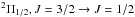 triplets, and 0.005 km -1 for the OH ground-state triplet. Data were smoothed to the values reported in Table 1 to increase the signal-to-noise ratio.
2.2. Herschel and APEX archive observations
The SOFIA observations presented in this paper are complemented by HIFI ([CII] (2P3/2−2P1/2), p-H2O (211−202), p-H2O (202−111), p-H2O (111−000), o-H2O (221−212), and o-H2O (212−101) and HF(1–0)) and APEX (CO(6−5) and CO(7–6)) archival data. The Herschel (Pilbratt et al. 2010) observations presented in this study were performed with the HIFI instrument (de Graauw et al. 2010). All APEX (Güsten et al. 2006) and Herschel data are centred at , , thus at an offset of (0″,2″) from the centre of the SOFIA data. We refer to van der Tak et al. (2013), Gusdorf et al. (2015), and Gerin et al. (2015) for the details of the H2O, [CII], and CO observations. The HF(1–0) data were acquired using the dual beam-switch observing mode in March, 2011. The data were processed with the standard HIFI pipeline using HIPE, and Level-2 data were exported using the HiClass tool available in HIPE. Further processing was performed in CLASS90. We assumed a flux scale accuracy of about 20% for the HIFI observations2 and for the APEX data (Gusdorf et al. 2015). For the Herschel HIFI data (obtained in the framework of the Guaranteed Time Key Programs PRISMAS and WISH, PIs: M. Gerin and E. van Dishoeck, respectively), we used the new measurements of Mueller et al. (2014) for the beam efficiencies and the beam sizes for Herschel observations performed with the HIFI receiver (see Table 1).
The angular and spectral resolutions of each dataset are reported in Table 1. The original spectral resolution is 0.08 km s-1 for the [CII] line, 0.15 km s-1 for p-H2O (202−111), 0.13 km s-1 for p-H2O (111−000), 0.09 km s-1 for o-H2O (221−212) and (212−101), 0.3 km s-1 for HF, and 0.27 km -1 for CO(7–6). Data were smoothed to the values reported in Table 1 to increase the signal-to-noise ratio.
3. Observational results
3.1. Atomic oxygen
 |
Fig. 2 [OI]63μm spectrum at the original resolution (6.̋6) of the SOFIA data extracted from the strongest continuum position (0″, + 3″ from |
Figure 2 shows the [OI]63μm spectrum at the original resolution (6.̋6) of the SOFIA data extracted from the strongest continuum position (0″, + 3″ from , ). The [OI]63μm profile is characterised by emission at high velocities (up to –40 km s-1 in the blue-shifted range, and +67 km s-1 in the red-shifted wing) and strong absorption at low velocities. The high-velocity emission covers a range very similar to that of other tracers, in particular, to that of water. We performed a spatial 2D Gaussian fit on the integrated intensity red- and blue-shifted high-velocity emission maps in the velocity ranges [+ 30, + 67] km s-1) and [−40,−2] km s-1). The results are summarised in Table 2. The high-velocity emission shows a similar distribution to the CO(6–5) emission recently mapped by Gusdorf et al. (2015) with the APEX telescope with an angular resolution of 9′′, but it is very compact compared to the CO(2–1) and (3–2) extremely high-velocity emission mapped by Su et al. (2012) with the SMA (Fig. 1). Both [OI]63μm red- and blue-shifted emissions peak very close to the position of Feldt’s star (see Fig. 3) with a relative offset between the two lobes of 1′′ along the north–south direction, as also found by Gusdorf et al. (2015) for CO(6–5). Thus, the high-velocity [OI]63μm emission probably arises from the unresolved outflows mapped by Su et al. (2012). Since the bandwidth of the GREAT receiver at 63 μm is limited to the band shown in Fig. 2, our data cannot provide information on the possible presence of [OI]63μm emission at extremely high velocities (up to –150 km s-1 at blue-shifted velocities and +90 km s-1 at red-shifted velocities) detected in CO(2–1) and (3–2) by Su et al. (2012).
The deep absorption at 2–15 km s-1 is due to the source itself and to a cold cloud along the line of sight at νLSR = 13.7 km s-1 (e.g., Klaassen et al. 2006), and it is completely saturated (the single-sideband continuum main-beam brightness temperature is 9.0 ± 0.7 K, see Table 3). This suggests a large amount of [OI] with low excitation conditions in the source, since the outer envelope of the source is completely absorbed. The features in absorption between [+ 19, + 25] km s-1 are due to foreground clouds along the line of sight (Flagey et al. 2013; van der Tak et al. 2013).
Results of the 2D Gaussian fit of the [OI]63μm integrated intensity and continuum distributions.
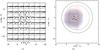 |
Fig. 3 a) Continuum-subtracted spectral map of [OI]63μm line in G5.89–0.39. The velocity range shown in the spectra ranges from −60 km s-1 to +100 km s-1. The temperature scale ranges from −10 K to + 20 K. b) Map of the continuum emission at 63 μm. Red and blue contours represent the integrated red- and blue-shifted intensity of the [OI]63μm line. For the continuum emission and for the red- and blue-shifted integrated intensities levels are 50% of the peak intensity (9.0 K for the continuum, 187.5 K km s-1 for the red wing, 422.0 K km s-1 for the blue wing) in steps of 10%. The star indicates the position of Feldt’s star, the cross the peak of the SOFIA 63 μm continuum emission, the triangles are the peaks of the red- and blue-shifted [OI]63μm emission (Table 2). The solid and dashed circles represent the 14.̋5 beam of the CO(16–15) data and the 11.̋6 beam of the OH ground-state observations. In both panels the centre position is |
Figure 4 shows the [OI]63μm spectrum smoothed to an angular resolution of 14.̋5 (that of the GREAT CO(16–15) data, Table 1) and comparisons with CO, H2O, OH, and [CII] lines smoothed to the same angular resolution where possible. The spectra are extracted at , δ[J2000]= .
.
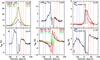 |
Fig. 4 Comparison of the [OI]63μm line profile from the central position of the map with other molecular and atomic features. The [OI]63μm, [CII], CO(6–5) and CO(7–6) spectra are extracted from a map smoothed to |

3.2. CO(16–15)
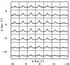 |
Fig. 5 Continuum subtracted spectral map of CO(16–15) in G5.89–0.39. Offsets are from the central position |
The CO(16–15) spectrum towards the central position of our map is shown in Fig. 4, while the spectral map is shown in Fig. 5. The red-shifted wing shows a narrow peak of emission at + 30 km s-1; given the spatial extent of this feature (see Fig. 5), this might be partially due to a telluric line that is not completely removed by our calibration procedure (Sect. 2.1.1). However, inspection of the HIFI CO(16–15) spectrum (Gusdorf et al. 2015,Fig. 14) reveals a weak peak at the same velocity, thus suggesting that the + 30 km s-1 feature in the SOFIA spectra is partially due to the telluric line and partially to a high-velocity peak. Figure 4 shows comparisons with the CO(6–5) and (7–6) smoothed to the same angular resolution of CO(16–15). High-velocity emission is detected in CO(16–15), although in a narrower range than in the mid-J CO lines, [OI]63μm, OH and H2O. This clearly indicates a decrease of excitation temperature with velocity (see Sect. 4.1.1).
3.3. Hydroxyl radical
Figure 4 shows the spectra of the blended hydroxyl radical (OH)  at 1834 GHz and 1837 GHz (detected in emission), and
  lines (detected in absorption) at 2514 GHz (see Table 1 for the exact frequencies). The triplets at 1837 GHz and 2514 GHz are partially resolved since they have a maximum separation of 14.7 km s-1 and 6.6 km s-1; on the other hand, the triplet at 1834 GHz is unresolved since the lines are separated by 2.4 km s-1 and the spectral resolution of this dataset is 1.5 km s-1 (see Table 1). The triplets at 1834 GHz and 1837 GHz have broad profiles with non-Gaussian red-shifted high-velocity emission in a velocity range similar to that seen in [OI]63μm and in the other molecular species. The hyperfine intensity ratios of the two triplets at 1834 GHz and 1837 GHz clearly deviate from the prediction of local thermal equilibrium (LTE) in the optically thin limit. The triplet at 2514 GHz is detected in absorption towards the continuum of the source at rest velocity and at blue-shifted high velocities. The foreground clouds at 20−25 km s-1 are also detected in absorption. Weak red-shifted emission is detected up to ~ + 70 km s-1 in agreement with the profiles of the other molecular and atomic features. The spectrum at 2514 GHz is complicated by the detection of the blue-shifted wing of the outflow of the second triplet at 2509 GHz, which falls into the lower sideband of the GREAT M channel and is seen in Fig. 4 at higher negative velocities than the 2514 GHz features. This complicates the determination of the continuum level in the spectrum. If we assume that the blue-shifted wing does not extend beyond −40 km s-1 (and indeed only [OI]63μm and mid-J CO are detected at such high velocities) and that the red-shifted profile does not cover velocities greater than + 85 km s-1 (not detected in any line except CO (2−1) and (3−2) by Su et al. 2012), we estimate a single-sideband continuum level of 6.7 ± 0.8 K in TMB units. The absorption around rest velocity and around + 25 km s-1 is saturated.
3.4. Hydrogen fluoride and ionised carbon
The spectrum of the hydrogen fluoride (HF) (1–0) line of G5.89−0.39 is presented in Fig. 6: the line shows three narrow (Δν ~ 3−7 km s-1) absorption features centred at 5.7 km s-1, 12.2 km s-1, and 20.5 km s-1, and a broad absorption at high velocities up to ν~−35 km s-1. At red-shifted velocities weak emission is maybe detected up to ~ + 50 km s-1, which could be caused by electron excitation, as suggested by van der Tak et al. (2012) for the Orion Bar. Given the tentative detection of emission in the red-shifted wing, we refrain from further analysis of HF at these velocities. The single-sideband continuum level of G5.89−0.39 is 5.1 ± 0.2 K in main-beam brightness temperature units, thus the absorption features at 12.2 km s-1, and 20.5 km s-1 are saturated.
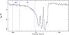 |
Fig. 6 HF(1–0) spectrum towards the position |
The ionised carbon ([CII]) fine structure  line in G5.89–0.39 is presented in detail by Gerin et al. (2015) and Gusdorf et al. (2015). It shows prominent high-velocity emission and absorption features associated with the source and with foreground gas at ~ + 20 km s-1 as in [OI]63μm, H2O, and OH. The continuum single-sideband brightness temperature is 10.5 ± 0.8 K.
3.5. Comparison of molecular and atomic spectra
In Fig. 4, the [OI]63μm spectrum from the central position of the map is compared with other molecular (CO, H2O, OH) and atomic ([CII]) features observed at comparable angular resolutions. The spectra are convolved to an angular resolution of 14.̋5 for the lines for which maps are available (see Table 1). For the lines observed with single pointings, the angular resolution ranges from 11.̋6 for the OH  triplet to 18.̋9 for p-H2O (111 → 000). In Fig. 3, we overlay the 14.̋5 beam size (angular resolution of most of the data) and the 11.̋6 beam of OH (the smallest) on the [OI]63μm blue- and red-shifted integrated intensity map to show that the [OI]63μm integrated intensity emission at 50% of the peak intensity is fully covered by our smallest beam. For clarity, the beam size of each spectrum is also indicated in Fig. 4.
The profiles of all spectral features shown in Fig. 4 are in all cases very similar and cover the same velocity range. The similarity of the line profiles strongly suggests that observations probe the same region despite the different angular resolutions. Based on the comparison of the CO(16–15) spectrum with the other profiles, we define four different velocity ranges: the low-velocity (LV) blue- ([−35,−2] km s-1) and red-shifted ([+ 32, + 47] km s-1) wings, which are detected in all spectral features (except for the blue-shifted LV in the OH  triplets); the high-velocity (HV) blue- ([−50,−35] km s-1) and red-shifted ([+ 47, + 65] km s-1) ranges, which are detected in all lines except CO(16−15) (red- and blue-shifted HV) and OH and [CII] (blue-shifted HV). We define the red-shifted LV range starting from + 32 km s-1 because the CO(16–15) [+ 28, + 30] km s-1 channels are contaminated by a narrow atmospheric feature (see Sect. 3.2).
Clearly, only lines with high critical densities (H2O transitions, HF(1–0), OH  ) are detected in absorption against the continuum of the source at blue-shifted velocities, while transitions with low critical densities ([OI]63μm, CO lines, [CII]) are detected in emission in the same velocity range. The OH
 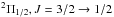 triplets, which have an upper level energy comparable to CO(7–6) but a much higher critical density, are the only lines not detected at blue-shifted high velocities. The detection of the OH triplets in the red-shifted non-Gaussian wing points to higher excitation conditions than in the blue-shifted lobe.
The similarities of the different line profiles are very well illustrated by Fig. 7 where the line ratio of different transitions to the [OI]63μm line is shown. The ratio is computed outside the velocity range [–2,+35] km s-1 and for the channels where the [OI]63μm line is above a 5 σ detection. To compute this ratio, we used the spectra shown in Fig. 4 convolved to an angular resolution of 14.̋5 for those lines where maps are available. For OH, and H2O, we smoothed the [OI]63μm data to the resolution of the other dataset. In both cases, we smoothed to a common velocity resolution of 2 km s-1. Except for the CO(6–5) lines, all other transitions have main-beam brightness temperatures lower than [OI]63μm at high velocities; however, all line ratios behave similarly and decrease with increasing velocity. The similarity of the profiles of OH and H2O is striking since in dissociative shocks [OI]63μm and OH are the main products of the destruction of water (e.g., Neufeld & Dalgarno 1989). CO and H2O lines transitions behave similarly as a function of velocity: the CO(6–5) and CO(16–15) to H2O at 1661 GHz line ratios are almost invariant with velocity from + 15 km s-1 (where the 1661 GHz line is no longer affected by absorption) to + 45 km s-1 (where the CO(16–15) line intensity falls below 3σ). The CO(6–5) to o-H2O (221 → 212) line ratio stays constant in the whole velocity range where the water line is detected above 3σ. These results differ from the findings of increasing H2O to CO line ratio with velocity in low-mass Class 0 and Class I sources based on the CO(3–2) and o-H2O ground-state lines (Kristensen et al. 2012), but fit the analysis of high-mass YSOs presented by San José-García (2015) for the CO(16–15) and (10–9) transitions, and the p-H2O 987 GHz line. These findings suggest that mid- and high-J CO lines (Jup> 6) and low-excitation H2O transitions originate in similar regions of the outflow system, probably in cavity walls (e.g., van Kempen et al. 2010; Visser et al. 2012).
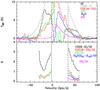 |
Fig. 7 Upper panel: [OI]63μm spectrum from the central position of the map compared with other molecular and atomic features. Lower panel: line ratio of CO(6–5) (black), CO(16–15) (red), [CII] (green), H2O 221−212 (blue), and the OH |
Single-sideband continuum levels.
4. Column densities and abundances at high velocity
4.1. Emission features
4.1.1. CO
Using the CO(6–5), (7–6) and (16–15) lines, we generated rotation temperature diagrams (Goldsmith & Langer 1999) in different velocity ranges to determine the average excitation temperature and column density of CO in a 14.̋5 beam under the assumption that the emission from these lines is optically thin. The results are presented in Table 4 and Fig. 8. There is a clear decrease of temperature with increasing velocities especially in the blue-shifted wing where the non-detection of CO(16–15) at HV constrains the excitation temperature to ≤ 68 K. Similarly, the red-shifted HV range infers temperatures lower than in the LV red-wing. In Table 4 we also report the values of Tex and NCO over the whole blue- ([−50,−2] km s-1) and red-shifted ([+ 32, + 70] km s-1) wings: these values agree well with the estimates for the warm component of Gusdorf et al. (2015) through the analysis of the whole CO ladder. Using the same method, these authors found a temperature of 270 K and a column density of 1017 cm-2 for both CO lobes by fitting CO lines up to Jup = 30 from APEX and Herschel-HIFI and -PACS.
We note that our result of decreasing temperature with velocity disagrees with the findings of Su et al. (2012), who determined a clear trend of increasing temperature with gas velocity based on interferometric CO(2–1) and (3–2) observations. Su et al. (2012) performed their analysis on much higher angular resolution (3.̋4 compared to our 14.̋5), and this disagreement could be due to dilution over our larger beam. However, given the small energy range covered by these two lines (ΔEu ~ 17 K), our dataset (ΔEu ~ 600 K) is probably better suited to constrain the average temperature of the outflowing gas in the region as a function of velocity, although compact hot gas at high velocities could be diluted in our beam in the CO(16–15) data.
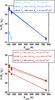 |
Fig. 8 CO rotational diagrams for different velocity ranges for the blue- (upper panel) and red-shifted (lower panel) emission over a beam size of 14.̋5, with an assumed filling factor value of 1. |
Results of the rotational diagrams for CO.
4.1.2. Atomic oxygen
Given the complexity of the [OI]63μm profile, we cannot use the PACS [OI]145 μm flux (Karska et al. 2014) to study the excitation of [OI] through the analysis of the [OI]63 μm to [OI]145 μm line ratio as done by other authors (e.g., Nisini et al. 2015). We therefore estimated the [OI] column density, N[OI], from the integrated intensity of the 63 μm line using the LTE approximation. Under this assumption, N[OI] is ![\begin{equation} \label{eq_coloi} N_{\rm{[OI]}}=\frac {8\pi k \nu^2}{h c^3 A_{\rm ul}}\times\frac{Q_{T_{\rm{ex}}}\exp(E_{\rm u}/kT_{\rm ex})}{g_{\rm u}}\int{T_{\rm{MB}}{\rm d}\varv}\frac{\tau}{1-\exp(-\tau)} , \end{equation}](/articles/aa/full_html/2015/12/aa26466-15/aa26466-15-eq149.png) (1)where QTex is the partition function, Tex is the excitation temperature, gu is the statistical weight of the upper level of the transition, Aul is the Einstein coefficient for spontaneous emission, and τ the optical depth of the 63 μm line. For the blue-shifted wing, assuming an excitation temperature of 200 K (as derived for CO) and without corrections for dilution, we derive an averaged optical depth of 0.06. This corresponds to an average column density over the 6.̋6 beam of ~ 1.2 × 1018 cm-2. For the red-shifted wing, the average column density over the 6.̋6 beam is ~ 5.7 × 1017 cm-2 with τ = 0.02 and Tex = 200 K. For a direct comparison with estimates of column densities of CO, OH, and H2, which are detected on larger scales, we also computed the average column density of [OI] on a 14.̋5 beam,
(1)where QTex is the partition function, Tex is the excitation temperature, gu is the statistical weight of the upper level of the transition, Aul is the Einstein coefficient for spontaneous emission, and τ the optical depth of the 63 μm line. For the blue-shifted wing, assuming an excitation temperature of 200 K (as derived for CO) and without corrections for dilution, we derive an averaged optical depth of 0.06. This corresponds to an average column density over the 6.̋6 beam of ~ 1.2 × 1018 cm-2. For the red-shifted wing, the average column density over the 6.̋6 beam is ~ 5.7 × 1017 cm-2 with τ = 0.02 and Tex = 200 K. For a direct comparison with estimates of column densities of CO, OH, and H2, which are detected on larger scales, we also computed the average column density of [OI] on a 14.̋5 beam, ![\hbox{$N_{\rm{[OI]}_{14\farcs5}}= 5.3\times10^{17}$}](/articles/aa/full_html/2015/12/aa26466-15/aa26466-15-eq158.png) cm-2 for the blue-shifted emission and
cm-2 for the blue-shifted emission and ![\hbox{$N_{\rm{[OI]}_{14\farcs5}}=2.1\times10^{17}$}](/articles/aa/full_html/2015/12/aa26466-15/aa26466-15-eq159.png) cm-2 for the red-shifted wing. Finally, we also report a [OI] column density of
cm-2 for the red-shifted wing. Finally, we also report a [OI] column density of ![\hbox{$N_{\rm{[OI]}_{12\farcs5}}=3.2\times10^{18}$}](/articles/aa/full_html/2015/12/aa26466-15/aa26466-15-eq160.png) cm-2 for the blue-shifted wing and of ~ 2.9 × 1018 cm-2 for the red-shifted wing. These values are integrated over a beam of 12.̋5 and corrected for a source size of 6.̋6. These estimates are used in Sect. 5 to derive the energetics parameters of the jet system and compare with similar estimates for the molecular outflows inferred by Gusdorf et al. (2015) on a 12.̋5 scale.
cm-2 for the blue-shifted wing and of ~ 2.9 × 1018 cm-2 for the red-shifted wing. These values are integrated over a beam of 12.̋5 and corrected for a source size of 6.̋6. These estimates are used in Sect. 5 to derive the energetics parameters of the jet system and compare with similar estimates for the molecular outflows inferred by Gusdorf et al. (2015) on a 12.̋5 scale.
We note, however, that the red-shifted flat profile suggests that the emission at these velocities has a very high optical depth since the profile is almost flat. Therefore, the column densities derived for the high-velocity red-shifted emission under the assumption of optically thin emission are lower limits to the real values. Under the assumption of extremely high optical depth, we can estimate the size of the red-shifted lobe assuming Tex = 200 K. The red-shifted observed main-beam brightness temperature corrected for the fact that the Rayleigh-Jeans approximation is not valid in this frequency and temperature regime is ~ 63 K. This implies a circular size of diameter 4.̋5 for the red lobe, in agreement with the findings of Sect. 3.1.
4.1.3. Ionised carbon
We determined the column density of [CII], N[CII], in the blue- and red-shifted wings based on the LTE assumption as done for [OI]63μm. Using Eq. (1) adapted for [CII], we obtain a [CII] column density of 3.6 × 1018 cm-2 in the blue-shifted wing of the spectrum (between −50 and −2 km s-1), and 1.2 × 1018 cm-2 in the red-shifted wing of the spectrum ([+32, +70] km s-1). These values are obtained over a beam size of 14.̋5 assuming optically thin emission, an excitation temperature of 200 K, and a source size of 12.̋5.
As already discussed by Gusdorf et al. (2015), [CII] is the dominant form of carbon in the warm outflowing gas.
4.1.4. H2O and OH
To determine the column density of OH and H2O at red-shifted velocities, we modelled their emission with the RADEX program (van der Tak et al. 2007), a radiative transfer code based on the large velocity gradient (LVG) approximation with a plane-parallel slab geometry. We investigated models with column densities ranging from 1013 cm-2 to 1018 cm-2, kinetic temperatures 25 K ≤ T ≤ 375 K, and densities in the range 103−108 cm-3. Ortho and para water were analysed separately and no assumptions on their relative abundance was made in the calculations. We considered a line width of 38 km s-1 (corresponding to the total velocity range [+ 32, + 70] km s-1 of the red-shifted emission), and a source size of 12.̋5 for all lines. This is based on the CO source size considered by Gusdorf et al. (2015). The molecular input files are taken from the LAMDA database (Schöier et al. 2005); for OH, we used entries that did not take into account the hyperfine structure because of the severe line overlap of the dataset. For both molecules, two solutions are found with similar values of the reduced χ2: the first gives column densities of some 1014 cm-2, high densities (≥ 107 cm-3), and temperatures higher than 100 K; the second solution implies high column densities (~ 1017 cm-2), low densities (n ≤ 106 cm-3), and no constraints on T. In neither case do the models fit the observations well for OH and p-H2O. This is most likely due to the simplifying assumptions made in the analysis (uniform temperature, density, and column density; common source size). Since the first solution matches the physical parameters derived from CO (see Sect. 4.1.1) fairly well, we chose this as the best fit to our data.
4.2. Absorption features
Since the blue-shifted wing of several molecular lines is detected in absorption against the corresponding continuum of G5.89–0.39, we can estimate the column density of OH, H2O, and HF at these velocities through the relation 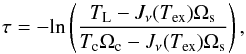 (2)where TL and TC are the brightness temperatures of the absorption line and of the continuum, Jν(Tex) is the Rayleigh-Jeans equivalent radiation field due to the molecular emission with excitation temperature Tex, Ωc and Ωs are the dilution factors for the continuum source and the blue-shifted outflow lobe, respectively. For the continuum we adopted the size derived at 63 μm (~ 12″, see Table 2) at the other frequencies, and we used a similar size (12.̋5) for the blue-shifted lobe as inferred from CO. From Eq. (2) we can also estimate an upper limit to the excitation temperature of the lines seen in absorption. We derive an upper limit of ~ 30 K and 25 K to the excitation temperatures of the 1661 GHz and 1669 GHz water lines, and of 14 K for the HF (1 → 0) transition. For H2O, we cannot use the 111 → 000 line at 1113 GHz because the line-to-continuum ratio in the blue-wing can only be reliably computed in a few channels. Assuming LTE conditions, the column density of the upper (Nu) and lower level (Nl) are related to the total column density Ntot of a molecule through
 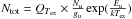 . The column density of a given molecule at a given excitation temperature can be derived in the same way as for [OI] (see Eq. (1), Sect. 4.1.2). Results are listed in Table 5. For the 1669 GHz line we used a lower excitation temperature (12 K) than the upper limit of 25 K because the column density at 25 K is too high compared to the value obtained from the 1661 GHz transition.
Column densities of different species and abundances relative to CO.
For the OH ground-state line, the hyperfine structure was modelled following Wiesemeyer et al. (2015), using the appropriate weights for the opacity of each component. Five velocity components were used to fit the line profile: one to fit the absorption at blue-shifted velocities from the outflow, two for the absorptions from different lines of sights and from the source envelope, and two to fit the red-shifted wing we see in emission. We used an excitation temperature of 10 K for the absorption features and of 200 K for the emission, in agreement with the estimates obtained from CO (Sect. 4.1.1). The central velocity and the line width of each component are free parameters of the fit, and the results are given in Table 6. Although only part of the triplet at 2509.9 GHz falls in the observed spectrum, the blue-shifted wing of this feature was used to constrain the fit. Similarly, the red-shifted emission was also included in the analysis; however, the velocity range ([–50, –2] km s-1) used to derive the OH column density in the blue-shifted lobe of the outflow is not influenced by the results of the red-shifted wing. The best fit of the OH ground-state triplet is shown in Fig. 9.
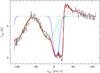 |
Fig. 9 Spectrum of the OH |
Fit results for the OH triplet at 2514 GHz.
4.3. Abundances
In Table 5 we report abundances of OH, H2O, and HF relative to CO for the blue- ([−50,−2] km s-1) and the red-shifted ([+ 32, + 70] km s-1) velocity ranges. Given the similarities of the line profiles, we assumed that all molecules trace the same gas. In the blue-shifted wing the water abundance relative to CO ranges between 2 × 10⁻¹ and 4 × 10⁻². Since Gusdorf et al. (2015) demonstrated that [CII] is the main form of carbon in G5.89−0.39 in the warm component, while CO and [CI] have similar column densities, we assumed that the total (CO+[CI]+C[II]) abundance of carbon relative to H2 is 1.4 × 10⁻⁴ and that the column density of [CI] is equal to that of the warm CO (Gusdorf et al. 2015). This results in H2O/H2 abundances of 10-7−10-6 in agreement with determinations in outflows from low-mass YSOs (e.g., Lefloch et al. 2010; Kristensen et al. 2012) but lower than in molecular outflows from massive YSOs (Emprechtinger et al. 2010; Leurini et al. 2014). The water abundance in the red-shifted lobe is one order of magnitude smaller than at blue-shifted HV (H2O/CO ~ 5 × 10⁻³, H2O/H2~ 3 × 10⁻⁸). For OH, we estimate an abundance relative to CO of (3−6) × 10-3, and of (1−3) × 10-8 relative to H2. The resulting OH to H2O abundance is 0.01 for the blue-shifted lobe, and 0.6 in the red-shifted velocity range. Given the large uncertainties in the estimates of the OH and H2O column densities, these abundances are consistent with models of fast dissociative J-type shocks (Neufeld & Dalgarno 1989) and of slower UV-irradiated C-type shocks (Wardle 1999). For HF, we derive an abundance relative to CO of 2 × 10⁻³ and of 10-8 relative to H2. While in the diffuse medium HF is an excellent tracer of molecular hydrogen (e.g. Neufeld et al. 2010; Monje et al. 2011) with a relative abundance to H2 of ~ 10-8 (Indriolo et al. 2013), the abundance of HF relative to H2 is not well constrained in dense environments, where depletion of F on grain surfaces is believed to play an important role (Phillips et al. 2010). Its abundance in molecular outflows from massive YSOs is even more uncertain: while Phillips et al. (2010) derived a lower limit to HF/H2 of 1.6 × 10⁻¹⁰ in Orion-KL, Emprechtinger et al. (2012) found 3.6 × 10⁻⁸ in AFGL 2591. Our measurement of the HF abundance in a molecular outflow from a massive YSO falls in between the two previous estimates.
[OI]63μm mass-loss rates and comparison with estimates from other tracers.
5. Mass-loss rate and energetics of the outflow system
The [OI] 63 μm line is expected to be the brightest atomic line in jets from YSOs because of the high abundance of atomic oxygen and favourable excitation conditions (e.g., Hollenbach & McKee 1989). For temperatures below 5000 K, Hollenbach (1985) suggested that the luminosity of the [OI] 63 μm line is directly proportional to the mass-loss rate from a protostar: ![\begin{equation} \label{hollenbach} \frac{\dot{M}}{M_\odot\,\mathrm{yr}^{-1}}= 10^{-4}\frac{L_{\rm[OI]\,63~\mu m}}{L_\odot} \cdot \end{equation}](/articles/aa/full_html/2015/12/aa26466-15/aa26466-15-eq238.png) (3)To allow the comparison with the estimates of the outflow energetics from CO, [CI] and [CII] from Gusdorf et al. (2015), we smoothed the [OI]63μm data to a resolution of 12.̋5. The corresponding [OI]63μm luminosities for the blue- and red-shifted wings are 4.8 L⊙ and 1.9 L⊙ (note that in Table 9LOI are reported on a 14.̋5 scale). We assumed that contamination of PDR emission at these velocities is negligible since the velocity range used for the integration starts at | v−vLSR | > 12 km s-1. The mass-loss rate estimates derived from Eq. (3) for the blue- and the red-shifted wings of [OI]63μm are reported in Table 7 together with the values from Gusdorf et al. (2015) based on CO, [CI] and [CII].
(3)To allow the comparison with the estimates of the outflow energetics from CO, [CI] and [CII] from Gusdorf et al. (2015), we smoothed the [OI]63μm data to a resolution of 12.̋5. The corresponding [OI]63μm luminosities for the blue- and red-shifted wings are 4.8 L⊙ and 1.9 L⊙ (note that in Table 9LOI are reported on a 14.̋5 scale). We assumed that contamination of PDR emission at these velocities is negligible since the velocity range used for the integration starts at | v−vLSR | > 12 km s-1. The mass-loss rate estimates derived from Eq. (3) for the blue- and the red-shifted wings of [OI]63μm are reported in Table 7 together with the values from Gusdorf et al. (2015) based on CO, [CI] and [CII].
Equation (3) relies only on the assumption that [OI]63μm is the dominant coolant of the gas in shocks with T< 5000 K. This assumption was verified to be valid for pre-shock densities n< 106 cm-3 by Hollenbach & McKee (1989). However, the shock models of Hollenbach & McKee (1989) most likely do not apply to massive star-forming regions since the UV radiation field from the protostar is completely neglected and preshock densities may be higher. Indeed, Gusdorf et al. (2015) verified that these models fail to reproduce the [CII] emission in G5.89−0.39 very likely because the only possible cause of dissociation is the UV field generated by the shock propagation itself. Moreover, the models of Hollenbach & McKee (1989) assumed a weak magnetic field, which is in contradiction with observations (Tang et al. 2009). Therefore, we also computed the mass-loss rate of the jet system in G5.89–0.39 directly as  (4)where td is the dynamical time of the outflow, and M the total mass in the outflow
 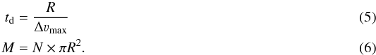 In Eqs. (5) and (6), R is radius of each lobe of the outflow assuming a circular size with a diameter of 6.̋6 because the [OI]63μm emission is mostly compact, Δνmax is the zero-intensity line width of the [OI] 63 μm line (Δνmaxblue = 50 km s-1 and Δνmaxred = 58 km s-1 assuming a rest velocity of 10 km s-1). The dynamical timescale of the [OI] outflow system is 350 yr for the red lobe and 400 yr for the blue lobe, in agreement with the estimate of Gusdorf et al. (2015) of 380 yr for both lobes based on CO. In Eq. (6), M is the total mass of the outflow and is derived over a 12.̋5 beam; N is the total column density of H2 at high velocities and is derived from the column density of [OI] assuming a relative abundance to H2. Our estimate of the mass of the red-shifted wing (and of the other parameters related to the energetics) is probably a lower limit since the [OI] column density at these velocities is determined under the assumption that the emission is optically thin, while the line profile suggests high opacities.
Gas-phase oxygen abundances between 3.07 × 10⁻⁴ and 4.85 × 10⁻⁴ are reported in the literature (e.g., Poteet et al. 2015; Baumgartner & Mushotzky 2006). Therefore, we adopted an oxygen abundance of 4 × 10⁻⁴ and assumed that all oxygen is in atomic form and in CO (whose column density is 1–4% of that of [OI], while those of H2O and OH are below 0.1%). The corresponding total column densities are 8.3 × 1021 cm-2 and 7.5 × 1021 cm-2 for the blue- and red-shifted lobes, respectively. The masses are 0.1 M⊙ for both lobes, and mass-loss rates 3.1 × 10⁻⁴M⊙ yr-1 and 3.2 × 10⁻⁴M⊙ yr-1 for the blue- and red-shifted lobes, in good agreement with the estimates based on Eq. (3) and on those based on CO, [CI], and [CII] from Gusdorf et al. (2015). This suggests that the assumption behind Eq. (3) (that the [OI]63μm is the main coolant at high velocities) also holds in massive jet systems. In Sect. 6 we investigate the contribution of several species to the far-IR line luminosity in different velocity ranges to confirm that [OI]63μm is the main coolant at high velocities.
The energetic of the jet system can be further characterised by estimating the momentum P, the mechanical force Fm, the kinetic energy Ek, and the mechanical luminosity Lm through 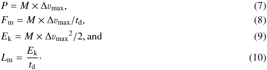 Results are summarised in Table 8. The parameters related to the energetics of the outflow agree well with those estimated by Gusdorf et al. (2015). However, our estimates are lower limits: no corrections for beam dilution or for the opacity of the [OI]63μm line were implemented in the calculation of the [OI] column density at blue-shifted velocities, and we have no estimates for the N[OI] column density in the red-shifted wing. Given these limits and the similar mass-loss rates found for the atomic jet and the molecular outflow, our results suggest that the molecular outflow system in the region is driven by the jet traced by [OI]63μm.
Jet parameters based on the [OI]63μm emission and comparison with outflow parameters from CO, [CI], and [CII] from Gusdorf et al. (2015) for the warm component.
Far-infrared line luminosities.
6. Far-infrared line luminosity
Far-infrared atomic and molecular features are commonly used to derive the gas cooling-budget in star-forming regions (e.g., Nisini et al. 2002; Karska et al. 2013, 2014). Following Karska et al. (2013, 2014), we define the total far-infrared line cooling (LFIRL) as the sum of the line emission luminosity from the atomic gas (from [OI] and [CII] in our case, L[OI] and L[CII], respectively) and from the molecular gas (H2O, CO and OH, L[H2O], L[CO], and L[OH]). In our analysis, we considered only spectral features with frequencies higher than 1000 GHz. When possible, we computed the luminosity of each species on datasets deconvolved to 14.̋5, the spatial resolution of the CO(16–15) data. OH and H2O observations are single pointings, but with resolutions similar to that of CO(16−15) (15.̋3 and 11.̋6 for OH at 1834−1837 GHz and 2514 GHz; 12.̋7 and 19.̋3 for H2O at 1661−1669 GHz and at 1113 GHz). The far-infrared line luminosity calculated in this way is a lower limit to its real value since it is based only on the spectral features presented in this paper. Table 9 summarises our results together with estimates from Karska et al. (2014), who analysed G5.89–0.39 in their sample of massive star-forming regions. Based on PACS observations of CO, H2O, OH, [OI], they derived a far-infrared line luminosity of 8.8 L⊙ for G5.89–0.39. The CO(16–15) transition is the strongest CO line in the PACS range and contributes to ~ 13% to the total CO luminosity. We find a CO(16–15) line luminosity integrated over the whole line profile of 0.65 L⊙, which agrees well with the results of Karska et al. (2014) (LCO(16−15) ~ 0.5 L⊙) if we consider that our beam is larger than the spaxel size (9.̋4) and that the CO emission is extended (Gusdorf et al. 2015). For the atomic gas, L[CII] was not analysed by Karska et al. (2014) because of contamination from the off position. The L[OI] from Karska et al. (2014) reported in Table 9 is only based on the 63 μm flux as in our study. We note that the 145 μm [OI] line does not contribute significantly to the total [OI] luminosity (Karska et al. 2014). Our higher L[OI63 μm] (5.7 L⊙) compared to Karska et al. (2014) (3.7 L⊙) is due to the larger beam used in our analysis. Indeed, on a 6.̋6 resolution, L[OI63 μm] is 3.4 L⊙, which agrees well with previous estimates. For the other species, a direct comparison between our results and those presented by Karska et al. (2014) is not straightforward. Values for single water lines are not reported in Karska et al. (2014), and the OH luminosity (LOH = 0.5 L⊙) is calculated from the triplets at 71 μm and 163 μm, while our estimate (0.44 L⊙) is based on the two triplets at 163 μm and on the ground-state lines at 119 μm at red-shifted high velocities. However, our findings generally agree well with Karska et al. (2014). On the spatial scale considered in our analysis (~ 20 000 AU), [OI] and CO (considering the whole far-infrared ladder from Karska et al. 2014) are the main contributors to the cooling. Water is 1% of LFIRL if we consider only the lines presented in this paper, and it accounts for up to 10% of the total cooling if we include the results of Karska et al. (2014). Therefore, water is a minor contributor to the total far-infrared line luminosity in this source. Finally, [CII] amounts to ~ 4% of the total line luminosity reported by Karska et al. (2014).
Given the high spectral resolution of all our datasets, we can determine the contribution of each species to the total cooling budget in different velocity regimes (see Table 9). While the total [OI]63μm luminosity is dominated by emission at blue-shifted velocities, the CO(16−15) luminosity arises almost equally from the blue- and red-shifted wings and from ambient velocities. If we assume that each of the three velocity components identified in CO (blue- and red-shifted emission, ambient emission) contributes to a third of the CO luminosity reported by Karska et al. (2014) over the whole ladder (as suggested by the CO(6−5), (7−6) and (16−15) lines, see also Gusdorf et al. 2015), the far-infrared line cooling budget of the outflowing gas is dominated by atomic oxygen at blue-shifted velocities. In the red-shifted wing, L[OI] and L[CO] are comparable. At ambient velocities, the far-infrared line cooling budget is dominated by CO as all other species are seen in absorption in this velocity range. The three water lines analysed in this study have a line luminosity of 0.1 L⊙ in the red-shifted wing, which makes water also a minor contributor to the total cooling in the outflowing gas.
7. Discussion
7.1. Atomic and molecular gas in jet/outflow systems
In Sect. 5 we found that the mass-loss rates estimated in G5.89−0.39 from [OI]63μm and from molecular gas are similar. The [OI]63μm mass-loss rate was estimated at high velocities (| v−vLSR | > 12 km s-1) assuming that PDR contamination is negligible (see van der Wiel et al. 2009; Pilleri et al. 2012, for typical line-widths in PDRs for different tracers). This suggests that the atomic jet in G5.89−0.39 is powerful enough to drive the larger scale molecular outflow(s). Similar comparisons between mass-loss rates from jets and molecular outflows were attempted in a few other massive YSOs with different jet tracers (SiO, H2, ionised gas). In IRAS 20126+4104 and IRAS 18151–1208, the jet seems to be driving the corresponding outflow (Cesaroni et al. 1999; Shepherd et al. 2000; Caratti o Garatti et al. 2008 for IRAS 20126+4104; Beuther et al. 2002; Davis et al. 2004 for IRAS 18151−1208), while in Ceph A and G192.16-3.82 the observed jets do not have enough momentum to support the outflows (Shepherd & Kurtz 1999; Rodriguez et al. 1994; Gómez et al. 1999).
The comparison of mass-loss rates derived from the atomic gas with molecular estimates also gives important constraints on the role of the atomic and molecular components in outflow/jet systems. Pioneering studies with ISO of outflows from low-mass YSOs compared mass-loss rates from CO with estimates from the [OI] 63 μm line (Ceccarelli et al. 1997; Giannini et al. 2001) and found that the two values agree fairly well despite the crude assumptions in the analysis of the [OI]63μm data. Recently, Herschel improved the situation by increasing the spatial resolution of [OI] 63 μm observations by a factor of ten. Nisini et al. (2015) analysed five jets from Class 0 low-mass YSOs and found that only in two sources the mass-loss rate from [OI]63μm is comparable with estimates based on CO, while in the other three cases Ṁ[OI] is more than an order of magnitude smaller than the corresponding Ṁ[CO]. The authors suggested that their results fit in an emerging scenario where jets from low-mass YSOs undergo an evolution in their composition with time: jets in the youngest sources would be mainly molecular, while the atomic component would become progressively more dominant as the jet gas excitation and ionisation increases (see also Podio et al. 2012) and would be dominant only in an intermediate phase of jet evolution. Our finding that the mass-loss rate from [OI]63μm is comparable with that from the molecular gas, and therefore that the atomic jet has an important role in driving the corresponding molecular outflow, could fit in this scenario since G5.89–0.39 already hosts an ultra-compact Hii region. However, the statistics on [OI]63μm in jets is too small to reach any solid conclusion: only a tenth of jets from low-mass protostars were mapped in [OI]63μm (Podio et al. 2012; Goicoechea et al. 2012; Nisini et al. 2015), and G5.89−0.39 is the first massive YSO observed in [OI]63μm with proper spectroscopic resolution to distinguish the contribution of high-velocity emission from ambient gas.
7.2. Quest for high-spectral resolution
Figure 4 shows that the [OI]63μm spectra in G5.89–0.39 are dominated by emission from the jet system, while the low-velocity range, most likely associated with PDR emission from the gas surrounding the ultra-compact Hii region, is severely contaminated by absorption features. Thus in G5.89–0.39, the PDR contribution to the [OI]63μm line is completely missing in the data.
Previous observations at lower spectral resolution (see for example Poglitsch et al. 1996; Liseau et al. 2006; Rosenberg et al. 2015) with KAO, ISO and Herschel suggested that the [OI]63μm transition may be considerably affected by absorption from foreground clouds and from the source envelope in different environments. These findings question the choice of [OI]63μm as a tracer of PDRs and of star-formation rates in external galaxies in case of spectrally unresolved lines. The case of G5.89–0.39 is exceptionally striking since Herschel PACS observations of the same region show a perfect Gaussian profile for the [OI]63μm with no hint of absorption (Karska et al. 2014,their Fig. 2) with a spectral resolution of 90 km s-1. The importance of absorptions in the line depends on the total column density of the source itself and on the position of the source in the Galaxy, which determines the number of intervening interstellar clouds along the line of sight to the source itself. Therefore, high-spectral resolution is in general a strong requirement for this kind of studies.
8. Conclusion
We reported the first high spectral resolution observations of the [OI] line at 63 μm. The target of our study was the inner part of the massive star-forming region G5.89–0.39, an ideal source to investigate the contribution of PDR emission, absorption features, and jet emission at high velocities since it hosts an ultra-compact Hii region and at least three outflows. We complemented the SOFIA [OI]63μm observations with spectroscopically resolved data from Herschel and APEX of the other major coolants of the gas (CO, OH, H2O, [CII]) to study their contributions to the total far-IR line luminosity in different velocity ranges. Our main results can be summarised as follows:
-
The [OI]63μm spectra are severely affected by absorption from thesource envelope and from intervening interstellar clouds alongthe line of sight. Emission is detected at high velocities. It iscompact and associated with the molecular outflows detectedalong the north-south direction in previous observations of CO.
-
The parameters of the jet system derived from the [OI]63μm agree well with those estimated for the warm molecular outflow system associated with the [OI] emission. This suggests that at least in this source the molecular outflow is driven by the atomic jet seen in [OI].
-
CO and [OI] contribute in a similar way to the total far-IR line luminosity of G5.89–0.39 when the full velocity range is considered. However, the [OI] emission is dominated by the high-velocity range, and indeed [OI] is the main contributor to the cooling budget of the gas at high velocities.
-
The line luminosity of the [OI] line at high velocities can be used as tracer of the mass-loss rate of the jet since [OI] is the main coolant of the gas in this velocity regime.
Our [OI]63μm observations clearly demonstrate that the 63 μm line can be heavily contaminated by absorption features from different clouds along the line of sight and that its line luminosity can be completely associated with jets in extreme sources such as G5.89–0.39. Therefore, its use as PDR and star-formation rate tracer might be limited if the profile of the line is not resolved. Velocity-resolved observations are now made be possible by the SOFIA telescope with the GREAT spectrometer and its upcoming high-frequency array up GREAT.
Acknowledgments
We like to thank an anonymous referee and Malcolm Walmsley for comments and suggestions that improved the clarity of the paper. We are grateful to Brunella Nisini and Linda Podio for helpful discussions and for allowing us access to their results before publication. This work is based in part on observations made with the NASA/DLR Stratospheric Observatory for Infrared Astronomy (SOFIA). SOFIA is jointly operated by the Universities Space Research Association, Inc. (USRA), under NASA contract NAS2-97001, and the Deutsches SOFIA Institut (DSI) under DLR contract 50 OK 0901 to the University of Stuttgart.
References
- Baumgartner, W. H., & Mushotzky, R. F. 2006, ApJ, 639, 929 [NASA ADS] [CrossRef] [Google Scholar]
- Beuther, H., Schilke, P., Sridharan, T. K., et al. 2002, A&A, 383, 892 [NASA ADS] [CrossRef] [EDP Sciences] [Google Scholar]
- Boreiko, R. T., & Betz, A. L. 1996, ApJ, 464, L83 [NASA ADS] [CrossRef] [Google Scholar]
- Büchel, D., Pütz, P., Jacobs, K., et al. 2015, IEEE Transactions on Terahertz Science and Technology, 5, 207 [CrossRef] [Google Scholar]
- Caratti o Garatti, A., Froebrich, D., Eislöffel, J., Giannini, T., & Nisini, B. 2008, A&A, 485, 137 [NASA ADS] [CrossRef] [EDP Sciences] [Google Scholar]
- Ceccarelli, C., Haas, M. R., Hollenbach, D. J., & Rudolph, A. L. 1997, ApJ, 476, 771 [NASA ADS] [CrossRef] [Google Scholar]
- Cesaroni, R., Felli, M., Jenness, T., et al. 1999, A&A, 345, 949 [NASA ADS] [Google Scholar]
- Coppin, K. E. K., Danielson, A. L. R., Geach, J. E., et al. 2012, MNRAS, 427, 520 [NASA ADS] [CrossRef] [Google Scholar]
- Dale, D. A., Helou, G., Brauher, J. R., et al. 2004, ApJ, 604, 565 [NASA ADS] [CrossRef] [EDP Sciences] [Google Scholar]
- Davis, C. J., Varricatt, W. P., Todd, S. P., & Ramsay Howat, S. K. 2004, A&A, 425, 981 [NASA ADS] [CrossRef] [EDP Sciences] [Google Scholar]
- de Graauw, T., Helmich, F. P., Phillips, T. G., et al. 2010, A&A, 518, L6 [NASA ADS] [CrossRef] [EDP Sciences] [Google Scholar]
- De Looze, I., Cormier, D., Lebouteiller, V., et al. 2014, A&A, 568, A62 [NASA ADS] [CrossRef] [EDP Sciences] [Google Scholar]
- Emprechtinger, M., Lis, D. C., Bell, T., et al. 2010, A&A, 521, L28 [NASA ADS] [CrossRef] [EDP Sciences] [Google Scholar]
- Emprechtinger, M., Monje, R. R., van der Tak, F. F. S., et al. 2012, ApJ, 756, 136 [NASA ADS] [CrossRef] [Google Scholar]
- Feldt, M., Puga, E., Lenzen, R., et al. 2003, ApJ, 599, L91 [NASA ADS] [CrossRef] [Google Scholar]
- Flagey, N., Goldsmith, P. F., Lis, D. C., et al. 2013, ApJ, 762, 11 [NASA ADS] [CrossRef] [Google Scholar]
- Gerin, M., Ruaud, M., Goicoechea, J. R., et al. 2015, A&A, 573, A30 [NASA ADS] [CrossRef] [EDP Sciences] [Google Scholar]
- Giannini, T., Nisini, B., & Lorenzetti, D. 2001, ApJ, 555, 40 [NASA ADS] [CrossRef] [Google Scholar]
- Goicoechea, J. R., Cernicharo, J., Karska, A., et al. 2012, A&A, 548, A77 [NASA ADS] [CrossRef] [EDP Sciences] [Google Scholar]
- Goicoechea, J. R., Etxaluze, M., Cernicharo, J., et al. 2013, ApJ, 769, L13 [NASA ADS] [CrossRef] [Google Scholar]
- Goldsmith, P. F., & Langer, W. D. 1999, ApJ, 517, 209 [NASA ADS] [CrossRef] [Google Scholar]
- Gómez, J. F., Sargent, A. I., Torrelles, J. M., et al. 1999, ApJ, 514, 287 [NASA ADS] [CrossRef] [Google Scholar]
- Guan, X., Stutzki, J., Graf, U. U., et al. 2012, A&A, 542, L4 [NASA ADS] [CrossRef] [EDP Sciences] [Google Scholar]
- Gusdorf, A., Gerin, M., Goicoechea, J. R., et al. 2015, submitted [Google Scholar]
- Güsten, R., Nyman, L. Å., Schilke, P., et al. 2006, A&A, 454, L13 [NASA ADS] [CrossRef] [EDP Sciences] [Google Scholar]
- Harvey, P. M., & Forveille, T. 1988, A&A, 197, L19 [NASA ADS] [Google Scholar]
- Heyminck, S., Graf, U. U., Güsten, R., et al. 2012, A&A, 542, L1 [NASA ADS] [CrossRef] [EDP Sciences] [Google Scholar]
- Hofner, P., & Churchwell, E. 1996, A&AS, 120, 283 [NASA ADS] [CrossRef] [EDP Sciences] [Google Scholar]
- Hollenbach, D. 1985, Conference on Protostars and Planets II, 61, 36 [Google Scholar]
- Hollenbach, D., & McKee, C. F. 1989, ApJ, 342, 306 [NASA ADS] [CrossRef] [Google Scholar]
- Hübers, H.-W., Eichholz, R., Pavlov, S. G., & Richter, H. 2013, J. Infrared, Millimeter, and Terahertz Waves, 34, 325 [Google Scholar]
- Hunter, T. R., Brogan, C. L., Indebetouw, R., & Cyganowski, C. J. 2008, ApJ, 680, 1271 [NASA ADS] [CrossRef] [Google Scholar]
- Indriolo, N., Neufeld, D. A., Seifahrt, A., & Richter, M. J. 2013, ApJ, 764, 188 [NASA ADS] [CrossRef] [Google Scholar]
- Karska, A., Herczeg, G. J., van Dishoeck, E. F., et al. 2013, A&A, 552, A141 [NASA ADS] [CrossRef] [EDP Sciences] [Google Scholar]
- Karska, A., Herpin, F., Bruderer, S., et al. 2014, A&A, 562, A45 [NASA ADS] [CrossRef] [EDP Sciences] [Google Scholar]
- Klaassen, P. D., Plume, R., Ouyed, R., von Benda-Beckmann, A. M., & Di Francesco, J. 2006, ApJ, 648, 1079 [NASA ADS] [CrossRef] [Google Scholar]
- Kraemer, K. E., Jackson, J. M., & Lane, A. P. 1998, ApJ, 503, 785 [NASA ADS] [CrossRef] [Google Scholar]
- Kristensen, L. E., van Dishoeck, E. F., Bergin, E. A., et al. 2012, A&A, 542, A8 [NASA ADS] [CrossRef] [EDP Sciences] [Google Scholar]
- Kurtz, S., Hofner, P., & Álvarez, C. V. 2004, ApJS, 155, 149 [NASA ADS] [CrossRef] [Google Scholar]
- Lefloch, B., Cabrit, S., Codella, C., et al. 2010, A&A, 518, L113 [NASA ADS] [CrossRef] [EDP Sciences] [Google Scholar]
- Leurini, S., Gusdorf, A., Wyrowski, F., et al. 2014, A&A, 564, L11 [Google Scholar]
- Liseau, R., Justtanont, K., & Tielens, A. G. G. M. 2006, A&A, 446, 561 [NASA ADS] [CrossRef] [EDP Sciences] [Google Scholar]
- Malhotra, S., Kaufman, M. J., Hollenbach, D., et al. 2001, ApJ, 561, 766 [Google Scholar]
- Monje, R. R., Phillips, T. G., Peng, R., et al. 2011, ApJ, 742, L21 [NASA ADS] [CrossRef] [Google Scholar]
- Motogi, K., Sorai, K., Habe, A., et al. 2011, PASJ, 63, 31 [NASA ADS] [Google Scholar]
- Mueller, M., Jellema, W., Olberg, M., Moreno, R., & Teyssier, D. 2014, HIFI-ICC-RP-2014-001 [Google Scholar]
- Müller, H. S. P., Thorwirth, S., Roth, D. A., & Winnewisser, G. 2001, A&A, 370, L49 [NASA ADS] [CrossRef] [EDP Sciences] [Google Scholar]
- Müller, H. S. P., Schlöder, F., Stutzki, J., & Winnewisser, G. 2005, J. Molec. Struct., 742, 215 [CrossRef] [Google Scholar]
- Neufeld, D. A., & Dalgarno, A. 1989, ApJ, 344, 251 [NASA ADS] [CrossRef] [Google Scholar]
- Neufeld, D. A., Sonnentrucker, P., Phillips, T. G., et al. 2010, A&A, 518, L108 [NASA ADS] [CrossRef] [EDP Sciences] [Google Scholar]
- Nisini, B., Giannini, T., & Lorenzetti, D. 2002, ApJ, 574, 246 [NASA ADS] [CrossRef] [Google Scholar]
- Nisini, B., Santangelo, G., Giannini, T., et al. 2015, ApJ, 801, 121 [NASA ADS] [CrossRef] [EDP Sciences] [Google Scholar]
- Paine, S. 2014 [Google Scholar]
- Phillips, T. G., Bergin, E. A., Lis, D. C., et al. 2010, A&A, 518, L109 [NASA ADS] [CrossRef] [EDP Sciences] [Google Scholar]
- Pickett, H. M., Poynter, I. R. L., Cohen, E. A., et al. 1998, J. Quant. Spectros. Rad. Transf., 60, 883 [Google Scholar]
- Pilbratt, G. L., Riedinger, J. R., Passvogel, T., et al. 2010, A&A, 518, L1 [CrossRef] [EDP Sciences] [Google Scholar]
- Pilleri, P., Fuente, A., Cernicharo, J., et al. 2012, A&A, 544, A110 [NASA ADS] [CrossRef] [EDP Sciences] [Google Scholar]
- Podio, L., Kamp, I., Flower, D., et al. 2012, A&A, 545, A44 [NASA ADS] [CrossRef] [EDP Sciences] [Google Scholar]
- Poglitsch, A., Herrmann, F., Genzel, R., et al. 1996, ApJ, 462, L43 [NASA ADS] [CrossRef] [Google Scholar]
- Poteet, C. A., Whittet, D. C. B., & Draine, B. T. 2015, ApJ, 801, 110 [NASA ADS] [CrossRef] [Google Scholar]
- Puga, E., Feldt, M., Alvarez, C., et al. 2006, ApJ, 641, 373 [NASA ADS] [CrossRef] [Google Scholar]
- Rodriguez, L. F., Garay, G., Curiel, S., et al. 1994, ApJ, 430, L65 [NASA ADS] [CrossRef] [Google Scholar]
- Rosenberg, M. J. F., van der Werf, P. P., Aalto, S., et al. 2015, ApJ, 801, 72 [NASA ADS] [CrossRef] [Google Scholar]
- San José-García, I. 2015, Ph.D. Thesis, University of Leiden [Google Scholar]
- Schöier, F. L., van der Tak, F. F. S., van Dishoeck, E. F., & Black, J. H. 2005, A&A, 432, 369 [NASA ADS] [CrossRef] [EDP Sciences] [Google Scholar]
- Shepherd, D. S., & Kurtz, S. E. 1999, ApJ, 523, 690 [NASA ADS] [CrossRef] [Google Scholar]
- Shepherd, D. S., Yu, K. C., Bally, J., & Testi, L. 2000, ApJ, 535, 833 [Google Scholar]
- Sternberg, A., & Dalgarno, A. 1995, ApJS, 99, 565 [NASA ADS] [CrossRef] [Google Scholar]
- Su, Y.-N., Liu, S.-Y., Wang, K.-S., Chen, Y.-H., & Chen, H.-R. 2009, ApJ, 704, L5 [NASA ADS] [CrossRef] [Google Scholar]
- Su, Y.-N., Liu, S.-Y., Chen, H.-R., & Tang, Y.-W. 2012, ApJ, 744, L26 [NASA ADS] [CrossRef] [Google Scholar]
- Tang, Y.-W., Ho, P. T. P., Girart, J. M., et al. 2009, ApJ, 695, 1399 [NASA ADS] [CrossRef] [Google Scholar]
- Tielens, A. G. G. M., & Hollenbach, D. 1985, ApJ, 291, 747 [NASA ADS] [CrossRef] [Google Scholar]
- van der Tak, F. F. S., Black, J. H., Schöier, F. L., Jansen, D. J., & van Dishoeck, E. F. 2007, A&A, 468, 627 [NASA ADS] [CrossRef] [EDP Sciences] [Google Scholar]
- van der Tak, F. F. S., Ossenkopf, V., Nagy, Z., et al. 2012, A&A, 537, L10 [NASA ADS] [CrossRef] [EDP Sciences] [Google Scholar]
- van der Tak, F. F. S., Chavarría, L., Herpin, F., et al. 2013, A&A, 554, A83 [NASA ADS] [CrossRef] [EDP Sciences] [Google Scholar]
- van der Wiel, M. H. D., van der Tak, F. F. S., Ossenkopf, V., et al. 2009, A&A, 498, 161 [NASA ADS] [CrossRef] [EDP Sciences] [Google Scholar]
- van Kempen, T. A., Kristensen, L. E., Herczeg, G. J., et al. 2010, A&A, 518, L121 [NASA ADS] [CrossRef] [EDP Sciences] [Google Scholar]
- Visser, R., Kristensen, L. E., Bruderer, S., et al. 2012, A&A, 537, A55 [NASA ADS] [CrossRef] [EDP Sciences] [Google Scholar]
- Wardle, M. 1999, ApJ, 525, L101 [NASA ADS] [CrossRef] [PubMed] [Google Scholar]
- Watson, C., Churchwell, E., Zweibel, E. G., & Crutcher, R. M. 2007, ApJ, 657, 318 [NASA ADS] [CrossRef] [Google Scholar]
- Wiesemeyer, et al. 2015, submitted [Google Scholar]
Appendix A: Correction for atmospheric absorption by mesospheric oxygen
The correction for atmospheric absorption of the spectra obtained with GREAT follows the usual procedure described in Guan et al. (2012). This concerns absorption due to water vapour and the quasi-continuous, collision-induced absorption by O2 and N2. For the telluric [OI] line at 63.2 μm only few spectra with high resolution exist. Since the width of the telluric [OI] line is ~ 1 kms-1, the corresponding spectral channels could simply be masked (e.g., Boreiko & Betz 1996). Here we followed a different approach. Since the telluric [OI] line originates in the mesosphere, we can approximate its radiative transfer by a single layer with a constant source function and absorption coefficient, that is,  (A.1)where TL,ν and Tatm,ν are the Rayleigh-Jeans equivalent values for the line temperature and mesopheric temperature, respectively. ηf = 0.97 is the forward efficiency of GREAT. This expression holds only for the [OI] line, contributions from the other atmospheric species are omitted because the standard calibration procedure already accounts for them. The transmission in the [OI] line, along the sightline through the stratosphere, thus becomes
  (A.2)Because of the mesospheric origin, the telluric [OI] line has a Gaussian profile,
  (A.3)where ν0 = 4744.77749 GHz is the line centre frequency, and Δν its full width at half-maximum. We obtain T0,ν and Δν from a least-squares fit to the line profile TL,ν. The Rayleigh-Jeans equivalent atmospheric temperature at ν0 is kept as a free parameter and adjusted in such a way that the extinction correction exp(τν) removes the telluric absorption in front of the [OI] line from G5.89–0.39. The only prerequesite needed here is that the spectrum be free from narrow components within ~ 2Δν from ν0, which is the case here. These calibration steps are shown in Fig. A.1.
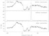 |
Fig. A.1 Top: 63.2 μm [OI] line of G5.89–0.39 after correction for the broad atmospheric absorption, but with the telluric [OI] line still uncorrected. Centre: Telluric [OI] emission line. Bottom: [OI] spectrum after the correction derived from a Gaussian fit to the telluric line. The continuum level is not corrected for the fact that GREAT operates in double-sideband. |
All Tables
Results of the 2D Gaussian fit of the [OI]63μm integrated intensity and continuum distributions.
Jet parameters based on the [OI]63μm emission and comparison with outflow parameters from CO, [CI], and [CII] from Gusdorf et al. (2015) for the warm component.
All Figures
|
Fig. 1 Overview (left) of the large scale east-west outflow and zoom (right) in the inner region powering the extremely high-velocity molecular outflows in CO(2–1) imaged with SMA from Su et al. (2012). The figures are adapted from Hunter et al. (2008) and Su et al. (2012). In the left panel, contours show the large-scale CO(1–0) outflow from Watson et al. (2007), pentagons are class I methanol masers (Kurtz et al. 2004), while crosses indicate the submillimetre-millimetre dust sources (Hunter et al. 2008). The dashed and dotted lines show the axes of the outflows detected at high velocities by Su et al. (2012). In the right panel, the red box delineates the region mapped in [OI]63μm; the red dots are the centres of the [OI]63μm raster map. The overlaid colour scale represents the cm free–free emission (Tang et al. 2009), filled triangles are the H2 knots, open circles are class I methanol maser positions, and open squares are positions of water masers (Hofner & Churchwell 1996). The crosses mark the position of the submillimetre-millimetre dust components. The ellipse shows the beam of the SMA observations from Su et al. (2012). |
| In the text | |
|
Fig. 2 [OI]63μm spectrum at the original resolution (6.̋6) of the SOFIA data extracted from the strongest continuum position (0″, + 3″ from |
| In the text | |
|
Fig. 3 a) Continuum-subtracted spectral map of [OI]63μm line in G5.89–0.39. The velocity range shown in the spectra ranges from −60 km s-1 to +100 km s-1. The temperature scale ranges from −10 K to + 20 K. b) Map of the continuum emission at 63 μm. Red and blue contours represent the integrated red- and blue-shifted intensity of the [OI]63μm line. For the continuum emission and for the red- and blue-shifted integrated intensities levels are 50% of the peak intensity (9.0 K for the continuum, 187.5 K km s-1 for the red wing, 422.0 K km s-1 for the blue wing) in steps of 10%. The star indicates the position of Feldt’s star, the cross the peak of the SOFIA 63 μm continuum emission, the triangles are the peaks of the red- and blue-shifted [OI]63μm emission (Table 2). The solid and dashed circles represent the 14.̋5 beam of the CO(16–15) data and the 11.̋6 beam of the OH ground-state observations. In both panels the centre position is |
| In the text | |
|
Fig. 4 Comparison of the [OI]63μm line profile from the central position of the map with other molecular and atomic features. The [OI]63μm, [CII], CO(6–5) and CO(7–6) spectra are extracted from a map smoothed to |
| In the text | |
|
Fig. 5 Continuum subtracted spectral map of CO(16–15) in G5.89–0.39. Offsets are from the central position |
| In the text | |
|
Fig. 6 HF(1–0) spectrum towards the position |
| In the text | |
|
Fig. 7 Upper panel: [OI]63μm spectrum from the central position of the map compared with other molecular and atomic features. Lower panel: line ratio of CO(6–5) (black), CO(16–15) (red), [CII] (green), H2O 221−212 (blue), and the OH |
| In the text | |
|
Fig. 8 CO rotational diagrams for different velocity ranges for the blue- (upper panel) and red-shifted (lower panel) emission over a beam size of 14.̋5, with an assumed filling factor value of 1. |
| In the text | |
|
Fig. 9 Spectrum of the OH |
| In the text | |
|
Fig. A.1 Top: 63.2 μm [OI] line of G5.89–0.39 after correction for the broad atmospheric absorption, but with the telluric [OI] line still uncorrected. Centre: Telluric [OI] emission line. Bottom: [OI] spectrum after the correction derived from a Gaussian fit to the telluric line. The continuum level is not corrected for the fact that GREAT operates in double-sideband. |
| In the text | |
Current usage metrics show cumulative count of Article Views (full-text article views including HTML views, PDF and ePub downloads, according to the available data) and Abstracts Views on Vision4Press platform.
Data correspond to usage on the plateform after 2015. The current usage metrics is available 48-96 hours after online publication and is updated daily on week days.
Initial download of the metrics may take a while.