| Issue |
A&A
Volume 583, November 2015
|
|
|---|---|---|
| Article Number | A124 | |
| Number of page(s) | 11 | |
| Section | Cosmology (including clusters of galaxies) | |
| DOI | https://doi.org/10.1051/0004-6361/201526531 | |
| Published online | 04 November 2015 | |
Ophiuchus: An optical view of a very massive cluster of galaxies hidden behind the Milky Way ⋆,⋆⋆
1 Sorbonne Universités, UPMC Univ. Paris 6 et CNRS, UMR 7095, Institut d’Astrophysique de Paris, 98bis Bd Arago, 75014 Paris, France
e-mail: This email address is being protected from spambots. You need JavaScript enabled to view it.
2 Faculty of Engineering, Gifu University, 1-1 Yanagido, 501-1193 Gifu, Japan
3 Department of Astrophysics, Nagoya University, Furocho, Chikusaku, 464-8602 Nagoya, Japan
4 LAM, OAMP, Pôle de l’Étoile Site Château-Gombert, 38 rue Frédéric Joliot–Curie, 13388 Marseille Cedex 13, France
5 INAF/Osservatorio Astronomico di Trieste, via Tiepolo 11, 34143 Trieste, Italy
Received: 14 May 2015
Accepted: 2 September 2015
Abstract
Context. The Ophiuchus cluster, at a redshift z = 0.0296, is known from X-rays to be one of the most massive nearby clusters, but its optical properties have not been investigated in detail because of its very low Galactic latitude.
Aims. We discuss the optical properties of the galaxies in the Ophiuchus cluster, in particular, with the aim of understanding its dynamical properties better.
Methods. We have obtained deep optical imaging in several bands with various telescopes, and applied a sophisticated method to model and subtract the contributions of stars to measure galaxy magnitudes as accurately as possible. The colour−magnitude relations obtained show that there are hardly any blue galaxies in Ophiuchus (at least brighter than r′ ≤ 19.5), and this is confirmed by the fact that we only detect two galaxies in Hα. We also obtained a number of spectra with ESO-FORS2, which we combined with previously available redshifts. Altogether, we have 152 galaxies with spectroscopic redshifts in the 0.02 ≤ z ≤ 0.04 range, and 89 galaxies with both a redshift within the cluster redshift range and a measured r′ band magnitude (limited to the Megacam 1 × 1 deg2 field).
Results. A complete dynamical analysis based on the galaxy redshifts available shows that the overall cluster is relaxed and has a mass of 1.1 × 10¹⁵ M⊙. The Sernal-Gerbal method detects a main structure and a much smaller substructure, which are not separated in projection.
Conclusions. From its dynamical properties derived from optical data, the Ophiuchus cluster seems overall to be a relaxed structure, or at most a minor merger, though in X-rays the central region (radius ~ 150 kpc) may show evidence for merging effects.
Key words: galaxies: clusters: individual: Ophiuchus / galaxies: photometry
Based on observations obtained with MegaPrime/MegaCam (program 10AF02), a joint project of CFHT and CEA/DAPNIA, at the Canada-France-Hawaii Telescope (CFHT), which is operated by the National Research Council (NRC) of Canada, the Institut National des Sciences de l’Univers of the Centre National de la Recherche Scientifique of France, and the University of Hawaii. Based on observations performed with ESO Telescopes at the La Silla Paranal Observatory under programme ID 085.A-0016(C). Based on observations obtained at the Southern Astrophysical Research (SOAR) telescope (programme 2009B-0340 on SOI/SOAR), which is a joint project of the Ministério da Ciência, Tecnologia, e Inovação (MCTI) da República Federativa do Brasil, the US National Optical Astronomy Observatory (NOAO), the University of North Carolina at Chapel Hill (UNC), and Michigan State University (MSU). This research has made use of the NASA/IPAC Extragalactic Database (NED), which is operated by the Jet Propulsion Laboratory, California Institute of Technology, under contract with the National Aeronautics and Space Administration, and of the SIMBAD database, operated at CDS, Strasbourg, France.
Tables A.1–A.3 are only available at the CDS via anonymous ftp to cdsarc.u-strasbg.fr (130.79.128.5) or via http://cdsarc.u-strasbg.fr/viz-bin/qcat?J/A+A/583/A124
© ESO, 2015
1. Introduction
Though the study of clusters is presently more often devoted to large surveys than to individual objects, it remains useful to analyse clusters individually when they appear to have particularly interesting or uncommon properties. The Ophiuchus cluster drew our attention because it is the cluster with the second brightest X-ray flux, but very little is known about it at optical wavelengths as a result of its very low galactic latitude.
Successful attempts have been made by several teams to detect extragalactic objects behind the Milky Way. First, Kraan-Korteweg (1989) searched for individual galaxies in the zone of avoidance at optical wavelengths, and subsequently published a series of papers with more detections, including clusters such as the Norma cluster (Kraan-Korteweg et al. 1996; Skelton et al. 2009). Nagayama et al. (2006) performed a near-infrared study of CIZA J1324.7-5736, the second richest cluster of galaxies in the Great Attractor. Ebeling et al. (2002) performed a systematic search for clusters (and even superclusters) of galaxies in X-rays; in this paper, these authors provide a first catalogue of 73 clusters at redshifts z< 0.26, and discuss the identification of the Great Attractor. Other X-ray detections were obtained by Lopes de Oliveira et al. (2006), who discovered Cl 2334+48 at z = 0.271 in the Zone of Avoidance in the XMM-Newton archive, and by Mori et al. (2013), who detected the rich cluster Suzaku J1759-3450 at z = 0.13 behind the Milky Way bulge. The latter cluster was then confirmed by Coldwell et al. (2014), based on infrared data.
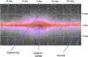 |
Fig. 1 2MASS near-infrared image of the Milky Way taken from the Aladin database, showing the positions of the Galactic centre and of the Ophiuchus and Norma clusters. |
At a redshift of 0.0296 (as inferred from our dynamical analysis, see Sect. 4.2), the Ophiuchus cluster was discovered in X-rays by Johnston et al. (1981), who identified the 4U 1708−23 X-ray source with a cluster of galaxies, and more or less simultaneously at optical wavelengths by Wakamatsu & Malkan (1981) during a search for highly absorbed Galactic globular clusters. The Ophiuchus cluster is located in the Zone of Avoidance, not very far from the Great Attractor.
Optical imaging observations.
Ophiuchus is mostly known for its X-ray properties since it is the cluster with the second highest X-ray flux after Perseus (Edge et al. 1990). Matsuzawa et al. (1996) obtained the first results with ASCA, by finding for the temperature and metallicity of the X-ray gas the respective values of kT = 9.8 keV and Z = 0.24Z⊙. Based on a mosaic of ASCA data, Watanabe et al. (2001) later derived that Ophiuchus was formed by the merging of two clusters with different iron abundances. They also detected the presence of a small group of galaxies with a colder temperature superimposed on the main cluster. Ophiuchus is part of the sample of clusters detected by Ebeling et al. (2002) in their systematic X-ray search for clusters behind the Milky Way. Ascasibar & Markevitch (2006) found that the X-ray emission map of Ophiuchus showed the presence of several sharp edges (see their Fig. 1), and argued that these could arise from gas sloshing, set up by a minor merger (as explained in detail by Markevitch & Vikhlinin 2007). The X-ray properties of the central part of Ophiuchus were also analysed in detail by Million et al. (2010), based on Chandra data. These authors showed the existence of a small displacement between the X-ray peak and the cD galaxy (~ 2 kpc), and of several strong features, such as sharp fronts and a very steep temperature gradient between the cool core (kT = 0.7 keV) and a region located only 30 kpc away (kT = 10 keV). All these properties suggest that the central regions of Ophiuchus (within 150 kpc of the cluster centre) show evidence for merging, whereas at radii larger than 150 kpc the cluster appears relatively isothermal with a constant metallicity. At even higher energies, Ophiuchus is also part of the sample of nearby clusters where evidence for indirect detection of dark matter has been searched for in Fermi gamma-ray data (Hektor et al. 2013).
Since Ophiuchus is very massive and very old (since it is in the nearby Universe), it can be considered a perfect example of a cluster in which the influence of the cluster on the member galaxies is as strong as can be in the Universe, and it can be taken as a reference for studies of galaxies in clusters such as red sequence or luminosity functions. Ophiuchus is also expected to be one of the clusters with very little star formation, and this motivated our attempt to detect star formation in Ophiuchus by observing it in a narrowband filter containing the Hα line at the cluster redshift. However, because of its low Galactic latitude Ophiuchus has not been observed much at optical wavelengths. An analysis was performed of the galaxy distribution at a very large scale (covering a 12° × 17° area) by Hasegawa et al. (2000), based on 4021 galaxies with measured spectroscopic redshifts. It was then shown by Wakamatsu et al. (2005) that Ophiuchus has a large velocity dispersion of 1050 ± 50 km s-1, agreeing with its high X-ray luminosity, and that several groups or clusters are located within 8° of the cluster, thus forming a structure comparable to a supercluster, close to the Great Attractor. They also found a large foreground void, implying that it is a continuation of the Local Void.
The difficulty of observing Ophiuchus at optical wavelengths is illustrated in Fig. 1, which indicates that it is even closer to the Galactic centre than the Norma cluster.
For a redshift of 0.0296, Ned Wright’s cosmology calculator1 gives a luminosity distance of 120.8 Mpc and a spatial scale of 0.585 kpc/arcsec, leading to a distance modulus of 35.54 (assuming a flat ΛCDM cosmology with H0 = 71 km s-1 Mpc-1, ΩM = 0.27 and ΩΛ = 0.73). The cluster centre is taken to be the position of the cD galaxy: RA = 258.1155°, Dec = −23.3698° (J2000.0). This is practically coincident with the peak of the X-ray emission, which is < 3 kpc (0.07 arcmin) away (Million et al. 2010).
The paper is organized as follows. We describe our optical data in Sect. 2. Results concerning the red sequence detected in colour−magnitude diagrams, star formation, internal structure, and dynamical properties are presented in Sect. 3. The cluster merging state is discussed in Sect. 4.
2. Optical imaging and spectroscopy
2.1. The data
We obtained optical images in various bands with several telescopes, as summarized in Table 1. At the Ophiuchus cluster redshift, the Hα line falls in the wavelength range covered by the filter adapted to observe the Galactic [SII]6717, 6731 emission, so we observed Ophiuchus in this filter with the SOAR telescope and SOI instrument during an observing run dedicated to galaxy clusters in 2009. We also took brief exposures in the Galactic Hα and R band filters to provide good continuum subtraction in deriving the Hα emission and the star formation rate in the galaxies belonging to the cluster.
2.2. Galaxy selection
As a pilot survey of galaxies, we chose an area of 10.1 × 9.3 arcmin2 in RA and Dec centred on the cD galaxy. This area covers the whole VLT and SOAR fields.
Initially, we tried an automated galaxy survey, but failed because too many blended stars were selected erroneously. Instead, we conducted our galaxy survey by eye inspection on the combined g′ and r′ band images by changing the image brightness and contrast on the ds9 and Gaia viewers. The detections of galaxies of small angular sizes are severely disturbed by many foreground stars. To overcome this difficulty, we performed a by eye inspection of the original images and of the star-subtracted images (see Sect. 2.3).
On these star-subtracted images, extended objects of small angular sizes show donut-shaped structures around their removed cores, while stars are clearly removed. This is our discrimination between stars and galaxies. For objects that are difficult to classify, we referred to stellarity indexes deduced from SExtractor and to results of image profiles measured with “imexamine” in IRAF. We selected 225 objects, and later closely re-examined 63 of these objects. Out of those 63 objects, 2/3 are found to be residuals around bright stars (see in Sect. 2.3) or objects with stellarity index > 0.15, and the remaining 1/3 are too faint to obtain reliable stellarity indexes. In Table A.1, we list 162 objects likely to be galaxies with their coordinates and magnitudes. Although the completeness of our survey is difficult to estimate in this complex area, we roughly estimate it to be higher than 70% for galaxies with angular sizes larger than 2.5 to 3 arcsec. Indeed, we independently performed a galaxy selection based on the VLT image, which has the best seeing, and found only two additional galaxies. We missed some small galaxies lying close to bright stars because they are buried in diffraction spiders and reflexion residuals of bright stars. Besides, some dwarf galaxies of low surface brightnesses with diameters larger than 3 arcsec are also missed because they are buried in irregularities of the sky background.
2.3. The method to subtract stars from the images
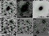 |
Fig. 2 Images illustrating our method for star subtraction. The field of view of each image is about 1.1 × 1.3 arcmin2 in the east-west and north-south directions, respectively. The small red circles indicate the position of the nucleus and the green ellipses represent the outer boundary of the galaxy. Top left a): original r′ band image of 2MASX J17121895-2322192 = OPH 171218.98-232219.1, one of the brightest galaxies. Bottom left b): stellar component after subtracting the galaxy model from image a). This image is almost free of galaxy light, and so it is appropriate for the evaluation of stellar parameters and measuring the PSFs. Top middlec): extracted galaxy image after automated star subtraction with PSFs. Since irregular residuals of saturated stars are not well removed, they disturb the galaxy profile and its surrounding sky area. Bottom middle d): image showing the automatically subtracted stars. This is the difference between images a) and c) and shows that more than 100 stars superposed on the galaxy are removed. Top righte): final image of the galaxy after manual cleaning of residuals around saturated stars in image c). Bottom rightf): residuals left after manual cleaning. This is the difference between images c) and e). |
On our r′ band Megacam image, the number density of foreground stars that disturb the galaxy surface photometry in Ophiuchus is about 350 stars arcmin-2, and therefore 100−200 stars are superposed on large bright galaxies. Hence, star subtraction is essential to achieve good quality galaxy photometry in Ophiuchus.
The present star subtraction procedure is a modified version of the method originally developed by Nagayama et al. (2006). It consists of 1) extraction of the point spread function (PSF); 2) star subtraction; and 3) cleaning of residuals such as those due to saturated stars or to diffraction on the spider. All these procedures were done using the DAOPHOT and STSDAS packages in IRAF.
We first describe the extraction of the PSF. Since almost all the stars that should be removed are blended with one another as a result of the high star density in the Galactic disk, a precise determination of the PSF is crucial. This requires isolated non-blended stars. However, almost all PSF candidate stars within an appropriate magnitude range are blended. Therefore, we obtained the final PSF after iterating three times the deblending process for these stars. We detected a spatial variation of the PSF even within a few arcminutes caused by the optics of the CFHT wide-field Megacam camera and the different performances of the mosaic CCDs of the camera. Therefore, star subtraction was processed by considering locally extracted PSFs.
Simple star subtraction from an original image is not appropriate, because the profiles of stars superimposed on a galaxy are disturbed by the light of the target galaxy. So, before star subtraction, the galaxy light should be removed from the original image by subtracting a brightness model of the galaxy. This model is extracted from a crude surface photometry of the galaxy with the “ellipse” and “bmodel” tasks in the IRAF STSDAS package. After subtracting this model galaxy from the original image, an image without the galaxy component is created (Fig. 2b). Based on this image, the stellar parameters for star subtraction with the series of PSFs are calculated with the “daofind”, “phot”, etc. tasks. By subtracting these stars from the original subimage with the “allstar” task, we then obtain a galaxy image without the superposition of foreground stars. Starting with this crudely removed galaxy image, we repeat this loop two or three times (Fig. 2c).
The automated star subtraction described above is almost perfect for non-saturated stars superposed on galaxies even if they are blended in a complicated way (Fig. 2c). However, this process works very poorly for saturated stars, which are always accompanied by large residuals, e.g. scattered light, spider diffraction patterns, etc. These have irregular shapes, therefore, we are obliged to remove them manually one by one with the “imedit” task in IRAF. If the outer annular zone encircling these residuals is clean and not disturbed by other residuals, the aperture around the residuals is replaced by an aperture interpolated from this boundary annulus with replacement option “b” in “imedit”. If replacement by interpolation is not appropriate because of neighbouring residuals or diffraction patterns, the residual aperture is substituted with the replacement option “m”, by a nearby aperture region of similar surface brightness to that of the galaxies (Fig. 2e). This cleaning process is the most delicate and painstaking job, since it must not modify the luminosity profiles and total magnitudes of the galaxies.
The error sources on the star subtraction processes for galaxy photometry are: 1) the subtraction of non-saturated stars with PSFs; 2) the replacement of residuals by interpolation and/or substitution as described above. Besides, bright stars located around the peripheries of galaxies cause uncertainty in the integration boundary for galaxy photometry. For elliptical and S0 galaxies that have smooth and symmetric structures, interpolation and substitution may not be a serious problem, but the situation is more difficult for spiral galaxies with knotty arms and for interacting galaxies with asymmetric tails and bridges. Fortunately, the Ophiuchus cluster is of cD type and therefore rich in E and S0 galaxies, and poor in spiral and interacting galaxies. To estimate errors in our photometric measurements, we considered two sets of images with different star subtractions, and obtained photometric measurements twice for each band. By comparing these two results, we estimate the errors in the three measured bands as follows:
-
0.07, 0.14, and 0.25 mag for objects with r′ < 19, 19 < r′ < 21, andr′ > 21, respectively;
-
0.08, 0.15, and 0.25 mag for objects with g′ < 20, 20 <g′ < 22, and g′> 22 respectively; and
-
0.05, 0.10, and 0.25 mag for objects with z′ < 20, 20 <z′ < 21, and z′ > 21 respectively.
These processes are illustrated in Fig. 2.
2.4. The photometric catalogue
After subtracting the star contribution (as described above), we extracted small subimages containing each galaxy and its immediate surroundings and measured magnitudes and morphological parameters with SExtractor (Bertin & Arnouts 1996). This was done in the g′, r′, and z′ bands for all the galaxies located in the field covered by the VLT/FORS2 image. Good quality measurements were achieved for 162 galaxies in the g′, r′, and z′ bands. In the region covered by Megacam but not by FORS2, only r′ band magnitudes were measured for the galaxies with spectroscopic redshifts to generate the largest possible sample of galaxies with both spectroscopic redshifts and magnitudes on which to apply the Serna & Gerbal analysis (see Sect. 3.3.3). The photometric catalogues are given in Tables A.1 and A.2.
2.5. The spectroscopic catalogue
Redshifts of bright galaxies were obtained covering a very large area on the sky with the AAO 6dF, CTIO 1.5 m and Lick 3 m telescopes (Wakamatsu et al. 2005), and these redshifts are listed in Table A.3. We also obtained spectroscopic data with the ESO VLT/UT1 telescope using FORS2 in two adjacent fields covering the very central region of the cluster, for a total exposure time of 1500 s. Spectra were obtained for 55 objects, out of which 54 gave reliable redshifts. Out of these, 17 proved to be galaxy spectra (about 14 belonging to the Ophiuchus cluster) and 37 were stars.
We retrieved redshifts in the NED data base in a region shown in Fig. 3. We also retrieved a spectrum of the cD galaxy taken by John Huchra at CTIO and measured its velocity at cz = 8844 ± 60 km s-1. This is within the error of the systemic velocity of the cluster 8878 ± 76 km s-1 (as inferred from the dynamical analysis, see Sect. 4.2).
We built a spectroscopic redshift catalogue by combining the Wakamatsu et al. (2005) measurements and our FORS2 measurements, and adding redshifts available in NED for galaxies that were not in the two previous catalogues. The resulting catalogue was limited to the redshift range 0.02 ≤ z ≤ 0.04, somewhat broader than the cluster range, in order not to lose galaxies. For the galaxies with several redshift measurements, we took the FORS2 value, the Wakamatsu et al. (2005) value, and the NED value in decreasing order of priority. Our final redshift catalogue is given in Table A.3 and includes 152 galaxies after eliminating objects with multiple measurements. We estimate the uncertainties in the corresponding cz velocities to be smaller than 280 km s-1 for the FORS2 data (see Adami et al. 2011) and between 100 and 300 km s-1 for the Wakamatsu et al. (2005) data. The spatial distribution of the galaxies with measured redshifts is shown in Fig. 3, and the redshift histogram is shown in Fig. 4.
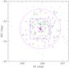 |
Fig. 3 Spatial distribution of the galaxies with spectroscopic redshifts, colour-coded as follows: magenta crosses: our FORS2 measurements; green crosses: Hasegawa measurements; and black crosses: values found in NED. The two magenta circles have radii of 0.5 deg (1 Mpc) and 1 deg (2 Mpc) and the blue square shows the size of the Megacam g′ and r′ band images. |
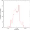 |
Fig. 4 Spectroscopic redshift histogram for the 152 galaxies of Table A3, with measured redshifts in the 0.02 ≤ z ≤ 0.04 redshift range. |
For the galaxies with spectroscopic redshifts located within the CFHT/Megacam field of view but outside the FORS2 field, we performed star subtraction and measured the magnitudes in the r′ band as described above. This yielded a catalogue of 89 galaxies with both redshifts and r′ band magnitudes within the 1 × 1 deg2 Megacam area, to which we applied the Serna-Gerbal software to search for substructures (see Sect. 3.3.3).
3. Results
3.1. The red sequence
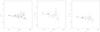 |
Fig. 5 Colour−magnitude diagrams. The red crosses are the galaxies with spectroscopic redshifts in the 0.02 ≤ z ≤ 0.04 range. |
For the galaxies with measured g′, r′ and z′ magnitudes, we drew the three possible colour−magnitude diagrams, which are shown in Fig. 5. We can see from the positions of the galaxies with spectroscopic redshifts in these diagrams that the red sequence is very well defined in all three plots. This confirms the validity of our photometric treatment and star subtraction.
The best fit to the (g′−r′) versus r′ relation computed with the galaxies brighter than r′ = 20 is  This relation can be compared to that estimated for a cluster of comparable richness and redshift, such as Coma. Eisenhardt et al. (2007) give the following relation for Coma (see their Table 13)
  If we translate our relation to B and R magnitudes using the Fukugita et al. (1995) transformations, we find for Ophiuchus,
  Though the slope for Ophiuchus is flatter than for Coma, the slopes are consistent within error bars, and the normalization parameters are of the same order of magnitude.
We also find from the colour−magnitude relations that there are very few bright blue galaxies in Ophiuchus: in the (g′−r′) versus r′ diagram, for example, there is not a single galaxy below the red sequence for r′ ≤ 19.5. This result is comparable to that found, for example, in the Coma cluster, where few galaxies bluer than the red sequence are detected (see Fig. 17 in Adami et al. 2007). This agrees with our idea that Ophiuchus is an old cluster, and this is also confirmed by the very small number of galaxies showing ongoing star formation (see next subsection).
3.2. Star formation in Ophiuchus galaxies
As explained in the introduction, we expect the majority of galaxies of Ophiuchus to be old, and therefore lacking star formation. To test this hypothesis, we observed the cluster in a narrowband filter containing Hα and [NII] at the cluster redshift, as explained in Sect. 2. We consider, in the following, Hα and [NII] as a single line noted Hα.
We first renormalize the Hα, [SII], and R band SOAR fluxes to take the different passbands of these filters and different exposure times into account.
For a given object in Ophiuchus, we denote as I the flux measured in the Hα filter. This flux includes the Milky Way Hα flux (MWHα) plus the continuum of the observed object at the filter wavelength (C1). We denote as II the flux received by the [SII] filter. This includes the Milky Way [SII] flux (MWSII), plus the Hα emission of the observed object (OHα), plus the continuum of the observed object at the filter wavelength (C2). These fluxes are calculated as follows:  Our goal is to measure the Hα emission of the observed object: OHα.
From Fig. 8 of Haffner et al. (1999), we estimate the ratio between the Milky Way Hα and [SII] emissions to be 4.7 ± 0.3 at the Ophiuchus position  (3)Moreover, we can safely assume that C1 ≃ C2, since the wavelengths of the Hα and [SII] filters are very similar, i.e.
  (4)Combining Eqs. (1) to (4), yields
  (5)We must now estimate C (our Hα and [SII] images and spectra are not flux calibrated). We assume this value to be the same for all the Ophiuchus galaxies, a reasonable hypothesis since we are considering a very homogeneous population of cluster galaxies. We then select the galaxies for which no Hα line is visible in our spectra. In this case, Eq. (5) becomes
  (6)We then estimate C for the previously selected Ophiuchus galaxies with no Hα emission, and apply this value to all the considered objects. We therefore have direct access to the uncalibrated OHα flux with Eq. (5) for all the observed objects.
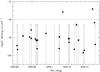 |
Fig. 6 Hα calibrated fluxes (in units of erg s-1 cm-2, in logarithmic scale) versus RA coordinates for all the galaxies detected along the Ophiuchus line of sight. Large open circles are the galaxies observed spectroscopically. The horizontal line shows the detection limit at 10-16 erg s-1 cm-2. |
To have a calibrated flux, we compare our SOAR R-band and CFHTLS r′ fluxes and apply the corresponding zero point to OHα fluxes. We then generate Fig. 6. Considering the galaxies for which we have a spectrum (we did not detect any Hα lines in our spectroscopic sample), we estimate the maximum value below which the Hα emission is not detectable to be about 10-16 erg s-1 cm-2.
Only two galaxies in Fig. 6 show a significant Hα emission. Their coordinates are (258.149°, −23.3223°) and (258.115°, −23.3696°) and their respective Hα fluxes are 1.45 × 10⁻¹⁵ and 0.69 × 10⁻¹⁵ erg s-1 cm-2.
After converting Hα fluxes into star formation rates (hereafter SFR) with the Kennicutt (1998) relation, our detection limit translates to 1.5 × 10⁻³ M⊙ yr-1, a fairly low value. Even the two galaxies in which we do detect Hα have fairly low SFRs of the order of 0.02 M⊙ yr-1 and 0.01 M⊙ yr-1 respectively.
We therefore conclude that the Ophiuchus galaxies have very low SFRs, as expected.
3.3. The cluster internal structure and dynamics
3.3.1. Selection of spectroscopic cluster members
We examined the positions of the galaxies in the blue peak (i.e. those with 0.02 ≤ z< 0.032) and those in the red peak (0.032 ≤ z ≤ 0.04) of Fig. 4, but were not able to separate them spatially. Therefore, if the blue and red distributions correspond to two clusters in the process of merging, the merger must take place along a direction close to perpendicular to the plane of the sky.
To identify the cluster members among the 152 galaxies with measured redshift, we use the “shifting gapper”method of Fadda et al. (1996). This method searches for gaps of 1000 km s-1 in the velocity distributions, within overlapping radial intervals of 0.4 h-1 Mpc (corresponding to 0.56 Mpc for our adopted cosmology). These gaps are used to separate interlopers from cluster members. Five galaxies are identified as interlopers with this procedure.
We then refine our membership identification using another procedure, which is similar to that developed by Biviano et al. (1996) for the Coma cluster. We determine two adaptive kernel maps of the galaxy number densities, one unweighted, and another weighted by the galaxy rest-frame velocities. The ratio of the two maps defines an adaptive kernel map of local velocities. We then run 1000 bootstrap resamplings to establish the significance of the adaptive kernel map of galaxy velocities, at each galaxy position, σboot,i (see Appendix A of Biviano et al. 1996, for more details). When the adaptive kernel value of the velocity at the ith galaxy position deviates from zero at more than 3σboot,i, we reject galaxy i from the list of cluster members. We reject five galaxies using this procedure, and, hence, we are left with a total of 142 cluster members. The projected-phase space distribution of all galaxies with spectroscopic redshifts in the cluster region is shown in Fig. 7. It shows a decrease of velocity dispersion with increasing distance from the cluster centre, as seen in many nearby clusters (e.g. Biviano et al. 1997).
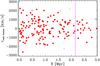 |
Fig. 7 Rest-frame velocities vs. distances from the cluster centre for all galaxies with redshifts in the cluster region. Filled (red) dots identify cluster members; the green-crossed red dot is the cD galaxy. The empty circles identify the five interlopers found via the shifting gapper procedure. The empty circles within squares identify the five interlopers found via the adaptive-kernel procedure. Some of these interlopers are nearly coincident in projected phase-space, hence the symbols are superposed. |
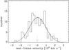 |
Fig. 8 Histogram of the rest-frame velocities of the identified cluster members. The best-fitting Gaussian is overplotted. The arrow indicates the velocity of the cD galaxy. |
3.3.2. Dynamical analysis
The histogram of rest-frame velocities for the cluster members is shown in Fig. 8. The mean redshift and velocity dispersion of the cluster members are  and
and  km s-1, respectively (derived using the robust biweight estimator; see Beers et al. 1990). Our new estimate of σv is significantly lower than the value obtained by Wakamatsu et al. (1050 ± 50 km s-1). Using our new values of
  and σv we draw the corresponding Gaussian distribution in Fig. 8. A Kolmogorov-Smirnov test (e.g. Press et al. 1992) yields a probability of 0.82 that the observed velocity distribution is a random draw of the Gaussian distribution. In other terms, the observed distribution is statistically indistinguishable from a Gaussian. This is generally taken as evidence for a relaxed dynamical configuration (e.g. Girardi et al. 1993; Ribeiro et al. 2011). Additional support for a dynamically relaxed status of the cluster also comes from the position of the cD in projected phase space (Beers et al. 1991). The position of the cD is in fact spatially coincident with the peak of the X-ray emission, and its velocity is consistent within the errors with the mean cluster velocity, Δv = 47 ± 97 km s-1.
It is possible to obtain a first, preliminary estimate of the cluster mass from the σv estimate, via the scaling relation of Munari et al. (2013; Eq. (1)): M200 = 9.3 [8.1,10.7] × 1014 M⊙, corresponding to r200 = 2.0 [1.89,2.07] Mpc, where the values in brackets correspond to the 1σ confidence intervals2. We proceed by estimating the cluster mass profile using the MAMPOSSt technique of Mamon et al. (2013). This technique performs a maximum likelihood fit of selected mass and velocity-anisotropy models to the projected phase-space distribution of cluster members.
We consider three models for the mass distribution: 1) Burkert (1995; “Bur”); 2) Hernquist (1990; “Her”); and 3) the popular Navarro et al. (1996; “NFW”). The three models are characterized by different logarithmic slopes of their mass density profiles, 0, −1, and −1 near the centre, and −3,−4,−3 at large radii, for Bur, Her, and NFW, respectively. Each of these models is characterized by two free parameters: the virial radius r200, and the scale radius. The NFW scale radius corresponds to the radius where the logarithmic slope of the mass density profile equals −2, and we therefore denote it by r-2. The Bur scale radius approximately corresponds to 2/3 r-2, while the Her scale radius corresponds exactly to 2 r-2. For the sake of homogeneity, we rescale the scale radii of the Bur and Her model to always quote the results for r-2.
We consider two models for the velocity anisotropy profile,  (7)where σθ,σφ are the two tangential components, and σr the radial component, of the velocity dispersion, and the last equivalence is obtained in the case of spherical symmetry. Negative, null, and positive values of β correspond to galaxy orbits, which are tangential, isotropic, and radial, respectively. One of the two models (“C”) assumes constant β(r) at all radii. The other (“T” from Tiret et al. 2007) is of the form: β(r) = β∞r/ (r + r-2). The two models are both characterized by only one free parameter, the constant value of β for the C model, and β∞ for the T model, since r-2 in this model is the same scale radius parameter of the mass models.
In MAMPOSSt and, in general, in all dynamical analyses based on the Jeans equation (Binney & Tremaine 1987), knowledge of the radial dependence of the completeness of the spectroscopic sample is required. An unknown, or uncorrected, radial dependence of the incompleteness would bias the determination of the number density profile of the tracer of the gravitational potential, which enters the Jeans equation. On the other hand, the velocity distribution of the tracers is in general unaffected by incompleteness problems since observations do not generally select cluster members in velocity space. In the case of Ophiuchus, an estimate of the radial completeness of the spectroscopic sample is not available because of the stellar crowded field. As a consequence, we must make the assumption that the number density profile of the tracers and the mass density profile of the cluster have the same shape, and are therefore characterized by the same scale parameter, r-2. This case was already considered by Mamon et al. (2013), and denoted TLM (for Tied Light and Mass). They showed that MAMPOSSt can also work very well within this restrictive assumption.
Results of the MAMPOSSt analysis.
We find that Her+T provides the best fit among the six combinations of the three mass and the two anisotropy models. However, all models are statistically acceptable. The best-fit values for the three free parameters r200,r-2,β∞ are listed in Table 2, with their uncertainties obtained by marginalizing each parameter with respect to the other two. For completeness, we also translate the constraints on r200 into constraints on the cluster mass, M200. The values of β∞ indicate that the galaxy orbits are mostly radially elongated in this cluster.
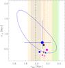 |
Fig. 9 Results of the dynamical analysis in the r-2 vs. r200 plane. The squares, dots, and triangles indicate the best-fit values obtained by MAMPOSSt for the Her, NFW, and Bur mass models. Magenta and blue symbols are for the C and T β(r) models, respectively. The symbol size is proportional to the MAMPOSSt likelihood. The ellipse indicates the 1σ uncertainty on the best-fit MAMPOSSt results, after marginalization over the velocity anisotropy parameter. The error bars are obtained upon marginalization of each parameter over the other two. The cross indicates the mean of the values obtained with the different models considered for the MAMPOSSt analysis. The vertical black dashed line indicates the value of r200 obtained from the cluster velocity dispersion using the scaling relation of Munari et al. (2013). The shaded grey region indicates the uncertainties in this value. The vertical red dash-dotted line indicates the value of r200 obtained with the Caustic technique of Diaferio & Geller (1997). The shaded orange region indicates the uncertainties in this value. The shaded green region indicates the range of r200 as obtained from the range of X-ray temperatures found in the literature (see text), using the scaling relation of Vikhlinin et al. (2009). The star symbol represents the theoretical expectation from De Boni et al. (2013), obtained adopting the average value of r200. |
In Fig. 9 we show the constraints obtained by MAMPOSSt in the r-2 vs. r200 plane. The uncertainties on the r200 value of the best-fit models, Her+T, are larger than the differences among the values obtained with the different models. On the other hand, some of the r-2 values are more than 2σ below the value obtained with the Her+T model. The average [r200,r-2] value (the + symbol in the figure) among the different models is in fact below the value of the best-fit model. However, it is remarkable that the latter is in excellent agreement with the theoretically predicted value obtained using the concentration-mass relation of De Boni et al. (2013; the star symbol in the figure), and the average value of r200 because the theoretical estimate comes from a concentration-mass relation. Given r200, one has the mass, and from the mass, the concentration. Given the concentration and r200, one has r-2.
We also show, in Fig. 9, the r200 values obtained from σv, using the scaling relation of Munari et al. (2013). The relatively narrow confidence region (grey shaded area in the figure) only reflects the uncertainty in the theoretical value of the scaling relation. In reality, this is an underestimate because several systematic uncertainties are not taken into account (see Munari et al. 2013, for more details). Considering that the formal uncertainties in the σv-determined r200 values are smaller than the real uncertainties, these values can be considered in fair agreement with the MAMPOSSt results.
The MAMPOSSt results are also in agreement with the r200 values obtained by applying the Caustic technique of Diaferio & Geller (1997; see also Diaferio 1999) to our spectroscopic data set (red line and orange shaded region in Fig. 9). This technique does not require the assumption of dynamical equilibrium, but suffers from an uncertain calibration, which is generally determined using numerical simulations. We adopt here the caustic mass calibration factor of Gifford et al. (2013), ℱβ = 0.65.
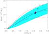 |
Fig. 10 Cluster mass profile as obtained from MAMPOSSt (solid blue line) within its 1σ confidence interval (dashed cyan region). The blue dot is the location of [r200,M200]. The dash-dotted and dashed red lines indicate the cluster mass profile obtained from the Caustic technique and, its 1σ upper and lower limits respectively. The red diamond is the location of [r200,M200]. The green X symbols indicate the locations of [r200,M200] obtained using the observed range of cluster TX and the scaling relation of Vikhlinin et al. (2009). |
Figure 10 shows the two mass profiles obtained by MAMPOSSt and the Caustic technique. They are in agreement within their uncertainties, except in the central region, where the Caustic mass profile exceeds the MAMPOSSt-derived mass profile. This is due to a well-known bias of the Caustic technique, which tends to overestimate the mass profile in the central regions (Serra et al. 2011). Overall we conclude that there is a very good agreement in the mass and mass profile estimates obtained with different techniques based on the projected phase-space galaxy distribution in the cluster.
It is also possible to determine r200 (and therefore also M200) from the cluster X-ray temperature. To accomplish this, we use the scaling relation of Vikhlinin et al. (2009) with fixed exponent α = 1.5 and the most recent and accurate determinations of the cluster X-ray temperatures, TX = 9.1 keV (Nevalainen et al. 2009) and TX = 9.7 keV (Fujita et al. 2008). The derived range of values accounts for the uncertainties in the normalization of the scaling relation of Vikhlinin et al. (2009). As can be seen from Figs. 9 and 10, the allowed range of r200 (and M200) values obtained from the X-ray temperatures, overlaps with the range of values we infer from the kinematic analysis. The X-ray derived values, however, tend to be somewhat higher than the values derived from the kinematic analysis. Possibly, the observed cluster TX is somewhat increased by a past collision between a cluster and a subcluster.
3.3.3. The presence of substructures
We performed a dynamical analysis with the Serna-Gerbal technique (hereafter SG, 1996 release, Serna & Gerbal 1996), a hierarchical code (based on spectroscopic redshifts and optical magnitudes) designed to detect substructures in the optical. The SG method has proved to be very powerful to show evidence for substructures in nearby clusters (see Abell 496: Durret et al. 2000; Coma: Adami et al. 2005; Abell 85: Boué et al. 2008) as well as in more distant clusters (Guennou et al. 2014). We applied it here to the catalogue of 89 galaxies with both redshifts and r′ band magnitudes within the 1 × 1 deg2 Megacam area.
Assuming a value of the mass to luminosity ratio (here taken to be 100), the SG method allows us to estimate the masses of the structures that it detects. Although the absolute masses are not accurate (the typical uncertainty is clearly larger than 1014 M⊙), the mass ratios of the various structures are well determined (Guennou et al. 2014). The SG method has also been extensively tested on simulations by Guennou (2012), in particular, concerning the effect of undersampling on mass determinations.
One of the parameters that can be chosen is the minimum number n of galaxies in a structure. We have applied the SG method with n = 10 and n = 5 and find similar results in both cases. The total mass of the system is found to be Mtot = 3.7 × 10¹⁴ M⊙. This estimate refers to the mass within the Megacam area, i.e. within a radius of ≃ 1 Mpc. We divide the masses of the detected substructures by this quantity to estimate the percentages of this total mass included in each of the substructures.
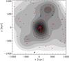 |
Fig. 11 Adaptive-kernel number density map of the galaxies in structure 1 of the SG substructure analysis. The contours are logarithmically spaced. Red dots indicate the positions of the galaxies belonging to this group. Blue stars indicate the positions of the galaxies belonging to group 2 in the SG substructure analysis. |
We find one large structure S1 of 75 galaxies and a much smaller structure S2 of 13 galaxies. The mass ratios of these two structures to the main cluster component are 0.67 and 0.065. Structure S1 can be divided into two substructures, S11 and S12, with 65 and 10 galaxies respectively, and S11 can itself be divided into two structures. In all cases, we find a large substructure and a much smaller one, implying that only minor mergers can be occuring. These results are illustrated in Fig. 11, where an adaptive kernel map of the main structure is drawn, with the galaxies of the two structures S1 and S2 superimposed.
As an illustration of the relative significance of the structures detected by the SG method, see Fig. 5 of Guennou et al. (2014), which shows the percentage of substructures detected by the SG method as a function of the spectroscopic sampling. The SG dynamical analysis therefore clearly confirms that Ophiuchus is not a fully relaxed cluster, but any merger must have been minor, and therefore has not strongly affected the dynamics of the cluster.
4. Discussion and conclusions
We now discuss the merging status of Ophiuchus. As mentioned above, only Watanabe et al. (2001) claim that it is a major merger based on a temperature map drawn from ASCA data. On the other hand, several studies, including ours, strongly suggest that Ophiuchus is only the result of a minor merger. From our data, there are several converging indices showing that Ophiuchus is not a cluster strongly perturbed by merging events. First, the centre of the cD galaxy coincides with the X-ray peak. Second, the velocity distribution is Gaussian, another evidence for global relaxation. Third, the cluster mass derived from the Jeans equation agrees with the cluster mass computed with the caustic method, which is still further evidence for relaxation. The masses derived from X-rays are a little higher, but still consistent. Finally, the SG analysis does not imply strong subclustering, given that a large fraction of the mass is not associated with any substructure.
Ophiuchus was originally believed to be a merging cluster, based on an X-ray temperature map derived from ASCA data (Watanabe et al. 2001), and shows two very hot regions to the west and south of the centre, some 20 arcmin away. The comparison of this map with simulations suggested that a merger had occurred about 1 Gyr ago. However, based on Suzaku data, these results were contradicted by Fujita et al. (2008), who did not detect the huge temperature variations found by Watanabe et al. (2001). On the contrary, they found that Ophiuchus was a cool core cluster, with isothermal gas (with a temperature  keV) beyond 50 kpc from the cluster centre. However, even if Ophiuchus is a cool core cluster, it may have experienced a minor merger, as indicated for example by the simulations of Burns et al. (2008). Fujita et al. (2008) also wrote that the iron-line ratios measured on the X-ray spectra indicated that the ICM had reached an ionization equilibrium state, implying that the cluster could not be a major merger. However, based on Chandra data, Million et al. (2010) found evidence for a collision from the comet-like morphology of the X-ray emission near the cluster centre. These authors interpreted the very strong temperature gradient, from 0.7 keV within 1 kpc to 10 keV at 30 kpc, as due to the fact that the outer part of the cool core has been stripped by ram pressure.
Other results are consistent with Ophiuchus being a minor merger. For example, Murgia et al. (2009) have detected a mini radio-halo around the cluster dominant radio galaxy, with a radio emissivity typical of haloes in merging clusters. However, according to Zandanel et al. (2014), the mini-halo in Ophiuchus has a radio luminosity much lower than giant radio halos in merging clusters, hence, this suggests that any merger can only have been a minor merger. The hard X-ray component detected with XMM-Newton by Nevalainen et al. (2009) is indicative of relativistic electrons, which are also responsible for the mini radio halo. The hypothesis of a minor merger is consistent with the fact that Hamer et al. (2012) measured an offset between optical line emission and the BCG (about 2 kpc), and suggested it could be due to the merger-induced motion of the ICM relative to the BCG. From their data, the merger must have occured recently, about 20−100 Myr ago.
Adding this evidence together, it seems likely that a merger has indeed occurred (probably rather recently), but that it was not a major merger, and perhaps since Ophiuchus is so massive, this merger has not perturbed its dynamical state much, though it may have affected the intra-cluster medium to some exent. At a smaller scale than the entire cluster, some perturbations have been observed. For example, an object, located 1.7 kpc from the BCG, shows low-ionization optical emission lines and is interpreted by Edwards et al. (2009) as a large cloud falling towards the BCG. This system would then be comparable to that described in the optical IFU observations of NGC 4696 by Farage et al. (2010). However, they cannot perturb the cluster properties, for example, as confirmed by the lack of star-forming galaxies.
The virial radius r200 is the radius of a sphere with mass overdensity 200 times the critical density of the Universe at the cluster redshift. The virial mass M200 is directly related to r200 via  , where Hz is the Hubble constant at the cluster mean redshift.
Acknowledgments
We thank A. Boselli for discussions and the referee for suggestions. F.D. acknowledges long-term support from CNES.
References
- Adami, C., Biviano, A., Durret, F., & Mazure, A. 2005, A&A, 443, 17 [NASA ADS] [CrossRef] [EDP Sciences] [Google Scholar]
- Adami, C., Durret, F., Mazure, A., et al. 2007, A&A, 462, A411 [NASA ADS] [CrossRef] [EDP Sciences] [Google Scholar]
- Adami, C., Mazure, A., Pierre, M., et al. 2011, A&A, 526, A18 [NASA ADS] [CrossRef] [EDP Sciences] [Google Scholar]
- Ascasibar, Y., & Markevitch, M. 2006, ApJ, 650, 102 [NASA ADS] [CrossRef] [Google Scholar]
- Beers, T. C., Flynn, K., & Gebhardt, K. 1990, AJ, 100, 32 [NASA ADS] [CrossRef] [Google Scholar]
- Beers, T. C., Gebhardt, K., Forman, W., Huchra, J. P., & Jones, C. 1991, AJ, 102, 1581 [NASA ADS] [CrossRef] [Google Scholar]
- Bertin, E., & Arnouts, S. 1996, A&AS, 117, 393 [NASA ADS] [CrossRef] [EDP Sciences] [Google Scholar]
- Binney, J., & Tremaine, S. 1987, in Galactic dynamics (Princeton University Press), 747 [Google Scholar]
- Biviano, A., Durret, F., Gerbal, D., et al. 1996, A&A, 311, 95 [NASA ADS] [Google Scholar]
- Biviano, A., Katgert, P., Mazure, A., et al. 1997, A&A, 321, 84 [NASA ADS] [Google Scholar]
- Boué, G., Durret, F., Adami, C., et al. 2008, A&A, 489, 11 [NASA ADS] [CrossRef] [EDP Sciences] [Google Scholar]
- Burkert, A. 1995, ApJ, 447, L25 [NASA ADS] [CrossRef] [Google Scholar]
- Burns, J. O., Hallman, E. J., Gantner, B., Motl, P. M., & Norman, M. L. 2008, ApJ, 675, 1125 [NASA ADS] [CrossRef] [Google Scholar]
- Coldwell, G., Alonso, S., Duplancic, F., et al. 2014, A&A, 569, A49 [NASA ADS] [CrossRef] [EDP Sciences] [Google Scholar]
- De Boni, C., Ettori, S., Dolag, K., & Moscardini, L. 2013, MNRAS, 428, 2921 [NASA ADS] [CrossRef] [Google Scholar]
- Diaferio, A. 1999, MNRAS, 309, 610 [NASA ADS] [CrossRef] [Google Scholar]
- Diaferio, A., & Geller, M. J. 1997, ApJ, 481, 633 [NASA ADS] [CrossRef] [Google Scholar]
- Durret, F., Adami, C., Gerbal, D., & Pislar, V. 2000, A&A, 356, 815 [NASA ADS] [Google Scholar]
- Ebeling, H., Mullis, C. R., & Tully, R. B. 2002, ApJ, 580, 774 [NASA ADS] [CrossRef] [Google Scholar]
- Edge, A. C., Stewart, G. C., Fabian, A. C., & Arnaud, K. A. 1990, MNRAS, 245, 559 [NASA ADS] [Google Scholar]
- Edwards, L. O. V., Robert, C., Mollá, M., & McGee, S. L. 2009, MNRAS, 396, 1953 [NASA ADS] [CrossRef] [Google Scholar]
- Eisenhardt, P. R., De Propris, R., Gonzalez, A. H., et al. 2007, ApJS, 169, 225 [NASA ADS] [CrossRef] [Google Scholar]
- Fadda, D., Girardi, M., Giuricin, G., Mardirossian, F., & Mezzetti, M. 1996, ApJ, 473, 670 [NASA ADS] [CrossRef] [Google Scholar]
- Farage, C. L., McGregor, P. J., Dopita, M. A., & Bicknell, G. V. 2010, ApJ, 724, 267 [NASA ADS] [CrossRef] [Google Scholar]
- Fujita, Y., Hayashida, K., Nagai, M., et al. 2008, PASJ, 60, 1133 [NASA ADS] [Google Scholar]
- Fukugita, M., Shimasaku, K., & Ichikawa, R. 1995, PASJ, 107, 945 [Google Scholar]
- Gifford, D., Miller, C., & Kern, N. 2013, ApJ, 773, 116 [NASA ADS] [CrossRef] [Google Scholar]
- Girardi, M., Biviano, A., Giuricin, G., Mardirossian, F., & Mezzetti, M. 1993, ApJ, 404, 38 [NASA ADS] [CrossRef] [Google Scholar]
- Guennou, L. 2012, Ph.D. Thesis, Université de Marseille-Provence, France [Google Scholar]
- Guennou, L., Adami, C., Durret, F., et al. 2014, A&A, 561, A112 [NASA ADS] [CrossRef] [EDP Sciences] [Google Scholar]
- Haffner, L. M., Reynolds, R. J., & Tufte, S. L. 1999, ApJ, 523, 223 [NASA ADS] [CrossRef] [Google Scholar]
- Hamer, S. L., Edge, A. C., Swinbank, A. M., et al. 2012, MNRAS, 421, 3409 [NASA ADS] [CrossRef] [Google Scholar]
- Hasegawa, T., Wakamatsu, K., Malkan, M., et al. 2000, MNRAS, 316, 326 [NASA ADS] [CrossRef] [Google Scholar]
- Hektor, A., Raidal, M., & Tempel, E. 2013, ApJ, 762, 22 [NASA ADS] [CrossRef] [Google Scholar]
- Hernquist, L. 1990, ApJ, 356, 359 [NASA ADS] [CrossRef] [Google Scholar]
- Johnston, M. D., Bradt, H. V., Doxsey, R. E., et al. 1981, ApJ, 245, 799 [NASA ADS] [CrossRef] [Google Scholar]
- Kennicutt, Jr. R. C. 1998, ARA&A, 36, 189 [Google Scholar]
- Kraan-Korteweg, R. C. 1989, Rev. Mod. Astron., 2, 119 [NASA ADS] [CrossRef] [Google Scholar]
- Kraan-Korteweg, R. C., Woudt, P. A., Cayatte, V., et al. 1996, Nature, 379, 519 [NASA ADS] [CrossRef] [Google Scholar]
- Lopes de Oliveira, R., Lima Neto, G. B., Mendes de Oliveira, C., Janot-Pacheco, E., & Motch, C. 2006, A&A, 459, 415 [NASA ADS] [CrossRef] [EDP Sciences] [Google Scholar]
- Mamon, G. A., Biviano, A., & Boué, G. 2013, MNRAS, 429, 3079 [NASA ADS] [CrossRef] [Google Scholar]
- Markevitch, M., & Vikhlinin, A. 2007, Phys. Rep., 443, 1 [NASA ADS] [CrossRef] [EDP Sciences] [Google Scholar]
- Matsuzawa, H., Matsuoka, M., Ikebe, Y., & Mihara, T. 1996, PASJ, 48, 565 [NASA ADS] [Google Scholar]
- Million, E. T., Allen, S. W., Werner, N., & Taylor, G. B. 2010, MNRAS, 405, 1624 [NASA ADS] [Google Scholar]
- Mori, H., Maeda, Y., Furuzawa, A., Haba, Y., & Ueda, Y. 2013, PASJ, 65, 102 [NASA ADS] [Google Scholar]
- Munari, E., Biviano, A., Borgani, S., Murante, G., & Fabjan, D. 2013, MNRAS, 430, 2638 [NASA ADS] [CrossRef] [Google Scholar]
- Murgia, M., Govoni, F., Markevitch, M., et al. 2009, A&A, 499, 679 [NASA ADS] [CrossRef] [EDP Sciences] [Google Scholar]
- Nagayama, T., Woudt, P. A., Wakamatsu, K., et al. 2006, MNRAS, 368, 534 [NASA ADS] [CrossRef] [Google Scholar]
- Navarro, J. F., Frenk, C. S., & White, S. D. M. 1996, ApJ, 462, 563 [NASA ADS] [CrossRef] [Google Scholar]
- Nevalainen, J., Eckert, D., Kaastra, J., Bonamente, M., & Kettula, K. 2009, A&A, 508, 1161 [NASA ADS] [CrossRef] [EDP Sciences] [Google Scholar]
- Press, W. H., Teukolsky S. A., Vetterling W. T., & Flannery B. P. 1992, Numerical Recipes in C, 2nd edn. (Cambridge University Press) [Google Scholar]
- Ribeiro, A. L. B., Lopes, P. A. A., & Trevisan, M. 2011, MNRAS, 413, L81 [NASA ADS] [Google Scholar]
- Serna, A., & Gerbal, D. 1996, A&A, 309, 65 [NASA ADS] [Google Scholar]
- Serra, A. L., Diaferio, A., Murante, G., & Borgani, S. 2011, MNRAS, 412, 800 [NASA ADS] [Google Scholar]
- Skelton, R. E., Woudt, P. A., & Kraan-Korteweg, R. C. 2009, MNRAS, 396, 2367 [NASA ADS] [CrossRef] [Google Scholar]
- Tiret, O., Combes, F., Angus, G. W., Famaey, B., & Zhao, H. S. 2007, A&A, 476, L1 [NASA ADS] [CrossRef] [EDP Sciences] [Google Scholar]
- Vikhlinin, A., Burenin, R. A., Ebeling, H., et al. 2009, ApJ, 692, 1033 [NASA ADS] [CrossRef] [Google Scholar]
- Wakamatsu, K., & Malkan, M. A. 1981, PASJ, 33, 57 [NASA ADS] [Google Scholar]
- Wakamatsu, K., Malkan, M. A., Nishida, M. T., et al. 2005, in Nearby Large-Scale Structures and the Zone of Avoidance, ASP Conf. Ser., 329, 189 [Google Scholar]
- Watanabe, M., Yamashita, K., Furuzawa, A., Kunieda, H., & Tawara, Y. 2001, PASJ, 53, 605 [NASA ADS] [Google Scholar]
- Zandanel, F., Pfrommer, C., & Prada, F. 2014, MNRAS, 438, 124 [NASA ADS] [CrossRef] [Google Scholar]
Appendix A: Catalogues
The photometric catalogue in the g′, r′, and z′ bands of the galaxies located within the VLT/FORS2 field is listed in Table A.1 for 162 objects.
The photometric catalogue in the r′ band of the galaxies with a measured spectroscopic redshift but outside the VLT/FORS2 field is listed in Table A.2 for 65 galaxies.
The full catalogue of 152 spectroscopic redshifts (covering a region larger than our images) is listed in Table A.3.
These Tables are available at the CDS.
All Tables
All Figures
|
Fig. 1 2MASS near-infrared image of the Milky Way taken from the Aladin database, showing the positions of the Galactic centre and of the Ophiuchus and Norma clusters. |
| In the text | |
|
Fig. 2 Images illustrating our method for star subtraction. The field of view of each image is about 1.1 × 1.3 arcmin2 in the east-west and north-south directions, respectively. The small red circles indicate the position of the nucleus and the green ellipses represent the outer boundary of the galaxy. Top left a): original r′ band image of 2MASX J17121895-2322192 = OPH 171218.98-232219.1, one of the brightest galaxies. Bottom left b): stellar component after subtracting the galaxy model from image a). This image is almost free of galaxy light, and so it is appropriate for the evaluation of stellar parameters and measuring the PSFs. Top middlec): extracted galaxy image after automated star subtraction with PSFs. Since irregular residuals of saturated stars are not well removed, they disturb the galaxy profile and its surrounding sky area. Bottom middle d): image showing the automatically subtracted stars. This is the difference between images a) and c) and shows that more than 100 stars superposed on the galaxy are removed. Top righte): final image of the galaxy after manual cleaning of residuals around saturated stars in image c). Bottom rightf): residuals left after manual cleaning. This is the difference between images c) and e). |
| In the text | |
|
Fig. 3 Spatial distribution of the galaxies with spectroscopic redshifts, colour-coded as follows: magenta crosses: our FORS2 measurements; green crosses: Hasegawa measurements; and black crosses: values found in NED. The two magenta circles have radii of 0.5 deg (1 Mpc) and 1 deg (2 Mpc) and the blue square shows the size of the Megacam g′ and r′ band images. |
| In the text | |
|
Fig. 4 Spectroscopic redshift histogram for the 152 galaxies of Table A3, with measured redshifts in the 0.02 ≤ z ≤ 0.04 redshift range. |
| In the text | |
|
Fig. 5 Colour−magnitude diagrams. The red crosses are the galaxies with spectroscopic redshifts in the 0.02 ≤ z ≤ 0.04 range. |
| In the text | |
|
Fig. 6 Hα calibrated fluxes (in units of erg s-1 cm-2, in logarithmic scale) versus RA coordinates for all the galaxies detected along the Ophiuchus line of sight. Large open circles are the galaxies observed spectroscopically. The horizontal line shows the detection limit at 10-16 erg s-1 cm-2. |
| In the text | |
|
Fig. 7 Rest-frame velocities vs. distances from the cluster centre for all galaxies with redshifts in the cluster region. Filled (red) dots identify cluster members; the green-crossed red dot is the cD galaxy. The empty circles identify the five interlopers found via the shifting gapper procedure. The empty circles within squares identify the five interlopers found via the adaptive-kernel procedure. Some of these interlopers are nearly coincident in projected phase-space, hence the symbols are superposed. |
| In the text | |
|
Fig. 8 Histogram of the rest-frame velocities of the identified cluster members. The best-fitting Gaussian is overplotted. The arrow indicates the velocity of the cD galaxy. |
| In the text | |
|
Fig. 9 Results of the dynamical analysis in the r-2 vs. r200 plane. The squares, dots, and triangles indicate the best-fit values obtained by MAMPOSSt for the Her, NFW, and Bur mass models. Magenta and blue symbols are for the C and T β(r) models, respectively. The symbol size is proportional to the MAMPOSSt likelihood. The ellipse indicates the 1σ uncertainty on the best-fit MAMPOSSt results, after marginalization over the velocity anisotropy parameter. The error bars are obtained upon marginalization of each parameter over the other two. The cross indicates the mean of the values obtained with the different models considered for the MAMPOSSt analysis. The vertical black dashed line indicates the value of r200 obtained from the cluster velocity dispersion using the scaling relation of Munari et al. (2013). The shaded grey region indicates the uncertainties in this value. The vertical red dash-dotted line indicates the value of r200 obtained with the Caustic technique of Diaferio & Geller (1997). The shaded orange region indicates the uncertainties in this value. The shaded green region indicates the range of r200 as obtained from the range of X-ray temperatures found in the literature (see text), using the scaling relation of Vikhlinin et al. (2009). The star symbol represents the theoretical expectation from De Boni et al. (2013), obtained adopting the average value of r200. |
| In the text | |
|
Fig. 10 Cluster mass profile as obtained from MAMPOSSt (solid blue line) within its 1σ confidence interval (dashed cyan region). The blue dot is the location of [r200,M200]. The dash-dotted and dashed red lines indicate the cluster mass profile obtained from the Caustic technique and, its 1σ upper and lower limits respectively. The red diamond is the location of [r200,M200]. The green X symbols indicate the locations of [r200,M200] obtained using the observed range of cluster TX and the scaling relation of Vikhlinin et al. (2009). |
| In the text | |
|
Fig. 11 Adaptive-kernel number density map of the galaxies in structure 1 of the SG substructure analysis. The contours are logarithmically spaced. Red dots indicate the positions of the galaxies belonging to this group. Blue stars indicate the positions of the galaxies belonging to group 2 in the SG substructure analysis. |
| In the text | |
Current usage metrics show cumulative count of Article Views (full-text article views including HTML views, PDF and ePub downloads, according to the available data) and Abstracts Views on Vision4Press platform.
Data correspond to usage on the plateform after 2015. The current usage metrics is available 48-96 hours after online publication and is updated daily on week days.
Initial download of the metrics may take a while.