| Issue |
A&A
Volume 583, November 2015
|
|
|---|---|---|
| Article Number | A65 | |
| Number of page(s) | 15 | |
| Section | Stellar structure and evolution | |
| DOI | https://doi.org/10.1051/0004-6361/201526216 | |
| Published online | 28 October 2015 | |
Rotation, differential rotation, and gyrochronology of active Kepler stars⋆
1 Institut für Astrophysik, Georg-August-Universität Göttingen, 37077 Göttingen, Germany
e-mail: This email address is being protected from spambots. You need JavaScript enabled to view it.
2 Max-Planck-Institut für Sonnensystemforschung, Justus-von-Liebig-Weg 3, 37077 Göttingen, Germany
Received: 30 March 2015
Accepted: 8 August 2015
Abstract
Context. In addition to the discovery of hundreds of exoplanets, the high-precision photometry from the CoRoT and Kepler satellites has led to measurements of surface rotation periods for tens of thousands of stars, which can potentially be used to infer stellar ages via gyrochronology.
Aims. Our main goal is to derive ages of thousands of field stars using consistent rotation period measurements derived by different methods. Multiple rotation periods are interpreted as surface differential rotation (DR). We study the dependence of DR with rotation period and effective temperature.
Methods. We reanalyze a previously studied sample of 24 124 Kepler stars using different approaches based on the Lomb-Scargle periodogram. Each quarter (Q1–Q14) is treated individually using a prewhitening approach. Additionally, the full time series and their different segments are analyzed.
Results. For more than 18 500 stars our results are consistent with the rotation periods from McQuillan et al. (2014, ApJS, 211, 24). Of these, more than 12 300 stars show multiple significant peaks, which we interpret as DR. Dependencies of the DR with rotation period and effective temperature could be confirmed, e.g., the relative DR increases with rotation period. Gyrochronology ages between 100 Myr and 10 Gyr were derived for more than 17 000 stars using different gyrochronology relations, most of them with uncertainties dominated by period variations. We find a bimodal age distribution for Teff between 3200–4700 K. The derived ages reveal an empirical activity-age relation using photometric variability as stellar activity proxy. Additionally, we found 1079 stars with extremely stable (mostly short) periods. Half of these periods may be associated with rotation stabilized by non-eclipsing companions, the other half might be due to pulsations.
Conclusions. The derived gyrochronology ages are well constrained since more than ~93.0% of the stars seem to be younger than the Sun where calibration is most reliable. Explaining the bimodality in the age distribution is challenging, and limits accurate stellar age predictions. The relation between activity and age is interesting, and requires further investigation. The existence of cool stars with almost constant rotation period over more than three years of observation might be explained by synchronization with stellar companions, or a dynamo mechanism keeping the spot configurations extremely stable.
Key words: stars: activity / stars: rotation / starspots
Full Tables 2 and 4 are only available at the CDS via anonymous ftp to cdsarc.u-strasbg.fr (130.79.128.5) or via http://cdsarc.u-strasbg.fr/viz-bin/qcat?J/A+A/583/A65
© ESO, 2015
1. Introduction
Encouraged by high-precision photometry of the CoRoT and Kepler satellites, measurements of stellar rotation periods have become numerous in recent years, unprecedented in their number and accuracy (Meibom et al. 2011a; Affer et al. 2012; McQuillan et al. 2013a,b, 2014; Nielsen et al. 2013; Walkowicz & Basri 2013; Reinhold et al. 2013). Owing to magnetic braking, the rotation period of a star is linked to its age. Stellar winds carry away charged particles along the magnetic field lines. As time proceeds, more and more material is dissipated, making the star slower and slower. This angular momentum loss over the star’s lifetime means that young stars rotate faster than old ones, on average.
A relation between stellar age and rotation period was first shown by Skumanich (1972). This author also demonstrated that the level of chromospheric activity depends on the stellar age. Succeeding measurements at the Mount Wilson Observatory corroborated the relations between chromospheric activity index  , the rotation period, and the stellar age (Noyes et al. 1984; Soderblom et al. 1991). Additionally, since the 1980s fast rotators are known to exhibit enhanced X-ray activity (Pallavicini et al. 1981; Pizzolato et al. 2003). These coherences are now established as activity-rotation-age relations.
Stellar ages cannot be measured directly but have to be inferred from other quantities. In principle, activity-age relations can be used to infer stellar ages, although their accuracy suffers from secular changes in the activity level. A classical method of inferring stellar ages is isochrone modeling. The ages of stellar clusters can be inferred from this method (see, e.g., Perryman et al. 1998), provided there is some knowledge of effective temperature, luminosity, and metallicity. This method can also be applied to field stars, however, with typical uncertainties on the order of 20–30%.
Over the past years, gyrochronology has become a promising way to derive stellar ages from their rotation periods (Barnes 2003, 2007, 2010; Mamajek & Hillenbrand 2008; Meibom et al. 2009, 2011b; Collier Cameron et al. 2009; James et al. 2010; Delorme et al. 2011). Barnes (2003, 2007) collected rotation periods from open clusters of different ages, and identified two sequences in the color-period diagram, namely the I- and C-sequence. Using known cluster ages, this author derived empirical fits to the color (mass) dependence of the data on the I-sequence, according to  (1)The function g(t) ∝ t1/2 is the rotation-age relation from Skumanich (1972), and f(B−V) an empirical fit to the (B−V)0 color dependence of the rotation period PI of the I-sequence stars reflecting their braking efficiency. Instead, (B−V)0 colors are used as a substitute for stellar mass. Unfortunately, gyrochronology is poorly calibrated for old stars. Meibom et al. (2011a) measured rotation periods for the 1 Gyr old cluster NGC 6811 in the Kepler field. The oldest star used for calibration was the Sun with an age of 4.55 Gyr. Bridging this large gap, Meibom et al. (2015) recently measured rotation periods of 30 stars in the 2.5 Gyr old cluster NGC 6819, deriving a well-defined period-age-mass relation. At later ages wide binaries might help to constrain the age-rotation relation (Chanamé & Ramírez 2012).
Another way to determine stellar ages is provided by asteroseismology (see, e.g., Chaplin et al. 2014). Recently, efforts are underway to calibrate asteroseismology ages by comparing them to gyrochronology measurements (García et al. 2014; do Nascimento et al. 2014; Lebreton & Goupil 2014; Angus et al. 2015). Furthermore, Vidotto et al. (2014) found a correlation between the average large-scale magnetic field strength and the stellar age according to ⟨ | BV | ⟩ ∝ t-0.655 similar to Skumanich’s law, calling this method magnetochronology. A review article on various age dating methods was provided by Soderblom (2010).
Gyrochronology relies on age calibration using open clusters of different ages, assuming their stars to be coeval. Calibration becomes difficult for clusters older than ~1 Gyr, however. One reason is that rotation periods are difficult to measure for slowly rotating stars. Furthermore, clusters become disrupted at that age (the degree strongly depends on the initial stellar cluster density), rendering the cluster membership of individual stars uncertain. Additionally, gyrochronology relations are calibrated only for main sequence dwarfs. Bulk rotation period measurements might be largely contaminated by subgiants (van Saders & Pinsonneault 2013), which have started evolving off the main sequence. Thus, applying gyrochronology relations using subgiant rotation periods might lead to a mis-classification of their evolutionary state (Doǧan et al. 2013).
Further uncertainties arise because a star is by no means a rigid rotator with a well-defined rotation period. High-precision instruments like the CoRoT and Kepler telescopes provide the opportunity to observe multiple rotation periods associated with latitudinal differential rotation (DR), which was observed for many active stars (Reinhold et al. 2013). Moreover, spot rotation periods heavily rely on their evolutionary timescales, which becomes more important for less active stars. Both effects may contribute large uncertainties to the rotation period used in the color-period fits.
Despite these drawbacks, gyrochronology relations supply a straightforward way to infer stellar ages of field stars. Other approaches to measure stellar ages are usually accompanied with large errors. Isochrone methods collapse for binary stars, which are assumed to be coeval, but do not appear on the same isochrone if the companions exhibit different masses. Asteroseismology ages strongly depend on some (usually unknown) model parameters (e.g., metallicity), which can lead to large errors.
The knowledge of stellar ages is of utmost interest for galactic formation. We aim to provide stellar ages for thousands of stars, inferred from mean rotation period measurements via gyrochronology. Furthermore, we show that multiple significant periods are quite common among active stars, which we assign to surface differential rotation. These period fluctuations dominate the age uncertainties. As opposed to this, we also found a subsample of stars almost showing no period variations over more than three years of observation.
The paper is organized as follows: Sect. 2 presents the Kepler data products. The different approaches used to analyze the data are explained in Sect. 3. Section 4 contains the results, which are further discussed in Sect. 5. We close with a brief summary of our results in Sect. 6.
2. Kepler data
The Kepler satellite provides almost continuous observations of the same field for more than four years (May 2, 2009−May 11, 2013). The data is delivered in quarters (Q0–Q17), each of ~90 d length (Q2–Q16), with exceptions for the commissioning phase Q0 (~10 d), and Q1 (~33 d). Unfortunately, observations stopped after one month of Q17 due to a failure of the third reaction wheel. This amazing amount of Kepler data is publicly available and can be downloaded from the MAST archive1.
Kepler data has been processed by different pipelines so far, starting with the Presearch Data Conditioning pipeline (PDC), designed to detect planetary signals. This pipeline was changed to the so-called PDC-MAP (Maximum A Posteriori) pipeline (Stumpe et al. 2012; Smith et al. 2012) because the PDC pipeline coarsely removed stellar variability signals. Recently, all Kepler data has been reprocessed by the PDC-msMAP (multiscale MAP) pipeline (Stumpe et al. 2014). This new version applies a 20-day high-pass filter intending to detect smaller planets in the data. Thus, this pipeline version is not suitable to look for stellar variability with a broad range of rotation periods since it diminishes stellar signals of slow rotators. Unfortunately, data reduced by previous pipeline versions are not publicly available anymore.
In Reinhold et al. (2013) we analyzed ~40 000 active stars with a variability range Rvar> 0.3% (for definition see Basri et al. 2010, 2011), only using Q3 data. In ~24 000 stars a clear rotation period was detected, and in ~18 000 stars a second period was detected, which was assigned to surface differential rotation. Starting from this sample, we extend our analysis to all available data. Our goal is to detect consistent rotation periods throughout the quarters, and to refine previous differential rotation measurements, exploiting the much higher frequency resolution thanks to the longer time span.
We do not use the much larger sample of 34 030 stars with measured rotation periods from McQuillan et al. (2014) because we are mostly interested in measuring DR. Although 20 009 stars of our sample are contained in the sample of McQuillan et al. (2014), the remaining stars either do not belong to the periodic sample of McQuillan et al. (2014), or have a smaller average variability range (Rvar< 0.3%), rendering them unsuitable for DR measurements.
In this work we only use Q1−Q14 PDC-MAP data (version 2.1 for Q1−Q4, Q9−Q11 and version 3.0 for Q5−Q8, Q12−Q14). Q0 data was discarded because of its short time span and the much lower number of monitored targets. From Q15 on, only PDC-msMAP data was available, which is unsuitable for our purposes as explained above.
Since we are only interested in rotation-induced stellar variability, we have to exclude targets showing other kinds of periodic variability. To reduce the number of false positives, i.e., periodic variability not related to stellar rotation, we discarded 17 eclipsing binaries2, 878 planetary candidates3, 2 RR Lyrae stars (Kolenberg et al. 2010; Szabó et al. 2010; Benkő et al. 2010; Guggenberger et al. 2012; Nemec et al. 2011, 2013; Moskalik et al. 2012; Molnár et al. 2012), and 84 γ Doradus and δ Scuti stars (Tkachenko et al. 2013; Ulusoy et al. 2014; Balona et al. 2011; Uytterhoeven et al. 2011; Lampens et al. 2013; Balona 2014). In total, 981 stars were discarded, leaving 23 143 targets, which are analyzed as described in the following section.
3. Methods
After excluding binarity stars and pulsators, we are interested in the stability of the rotational modulation. Many effects can change the shape of a light curve dominated by star spots rotating in and out of view, e.g., spots are created, others disappear while rotation takes place. The number of spots and their sizes are usually unknown. Differential rotation further hampers the detection of stable rotation periods. Sun spots change their preferred latitude of occurrence during the solar activity cycle, and therefore their rotation rate. But cyclic variability is also expected in other active stars. Moreover, Kepler suffers from instrumental effects, which are corrected by the pipeline automatically. Improper correction can mimic long-term (periodic) variability. The Kepler satellite rolls between consecutive quarters to reorientate its solar arrays. Hence, in each quarter stars fall on different CCDs with different sensitivity.
To account for all these effects, we analyze the data of the same star in different ways. First, we apply our analysis to each quarter individually. By comparing periods of individual quarters among themselves, we shrink our initial sample to find stable rotation periods among many quarters. After that, we stitch together data from all quarters for each star in our sample, and apply a slightly different period search to the full light curve. In a last step, we analyze different segments of the full light curve because some effects, (e.g., differential rotation) are more visible in certain segments rather than in the full time series. By comparing the periods returned by each method, we hope to detect stable rotation periods, which are unlikely caused by instrumental systematics.
3.1. Analysis of individual quarters
To detect periodic signals in the data we use the Lomb-Scargle periodogram in a prewhitening approach as described in Reinhold et al. (2013). Each quarter is analyzed individually and in the same way. The analysis method in briefly summarized below. For details we refer the reader to the paper mentioned above.
For each star and each quarter we compute the variability range Rvar,Q. If Rvar,Q> 0.3% holds for a certain quarter, we compute five Lomb-Scargle periodograms in a successive prewhitening approach. Since computing the Lomb-Scargle periodogram is equivalent to fitting a sine wave to the data, each prewhitening step yields a set of sine fit parameters (period Pk, amplitude ak, phase φk, and a total offset c) for k = 1,...,5. The parameters which belong to the highest peak in the periodogram yield the best parameters to fit the data. We use the returned values as initial parameters for a global sine fit to the data (t,y) according to 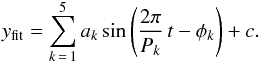 (2)This global sine wave is fit to the data through χ2-minimization. To save computation time each light curve was binned to two hours cadences. The period associated with the highest peak in the Lomb-Scargle periodogram is called P1, and represents the most significant period in the data.
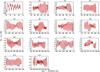 |
Fig. 1 Light curves (black) and sine fits (red) according to Eq. (2) of the star KIC 1163579 for all quarters Q1–Q14. Period measurements of this star are given in Table 1. |
In some cases spots are located on opposite sides of the star, and only half of the true rotation period is detected. To reduce this number of alias periods we compare P1 to the set of periods Pk and their corresponding peak heights hk: = h(Pk). If it holds  (3)then the period Pk is likely the true rotation period. In case P1 already was the correct period, we check if there are periods Pk satisfying
  (4)If that is not the case, the period Pk is used as rotation period, and we call this rotation period P1.
Since our primary goal is to detect differential rotation, we look for periods adjacent to P1. A probable second period should satisfy  (5)The period Pk with the second highest power in the prewhitening process satisfying Eq. (5) is called P2. In the following section we compare period measurements of individual quarters among themselves.
3.1.1. Comparison of periods from different quarters
As discussed at the beginning of Sect. 3, the measured periods P1 may change from quarter to quarter. That is especially true for stars exhibiting a second period P2 because spots may have changed their location, size, or occurrence at all. In addition, the period P2 might be a spurious detection in some quarters. As a first step, we look for stars with stable rotation periods throughout the quarters. Picking and choosing the best stars shrinks our primary sample, but provides a more reliable measure of the mean stellar rotation period, and eventually the stars’ DR.
For each star and each quarter Q = 1,...,14 we compute the variability range4Rvar,Q. If Rvar,Q> 0.3% we apply our prewhitening approach, which yields a period P1,Q. If Rvar,Q< 0.3%, or the star was not monitored in a certain quarter, the period P1,Q is set to zero. We only consider periods satisfying 0.5 d <P1,Q< 45 d. The upper limit accounts for the (at least) two full rotation cycles that we like to see during the limited quarter length of ~90 days. The lower limit should exclude pulsating stars. We compute the relative deviation of the periods P1,Q from their median according  . Fast rotators with a median period
  d are allowed to differ by 10%, stars with longer periods by 20%. From all periods P1,Q satisfying these criteria, we define a mean rotation period ⟨ P1 ⟩. If more than 75% of the periods P1,Q satisfy this criterion, the star belongs to the so-called good sample. The good stars are shown in Fig. 6 compared to previous measurements for the whole sample. We also checked for alias periods among our set P1,Q according to Eq. (4), but without comparing any peak heights. Periods identified as such were discarded. The star KIC 1163579, randomly chosen from our sample, is shown in Fig. 1, and its briefing is shown in Table 1. In the following section we concatenate data from individual quarters to analyze the full light curve.
3.2. Analysis of the full time series
In the previous section we only considered periods shorter than 45 days, due to the limited quarter length of ~90 days. Stitching together data from all available quarters is the only way to achieve two major goals: 1) the detection of periods longer than 45 days; and 2) to obtain a higher frequency resolution in the Lomb-Scargle periodogram, since the peak width scales with the inverse of the time span.
The first point is difficult to address. As mentioned earlier long-term instrumental effects are sometimes difficult to distinguish from slow rotation, especially in an automated period search of a large sample of objects. Furthermore, for this particular sample rotation periods of less than 45 days were measured in Reinhold et al. (2013). Measurements of alias periods or spurious detections are possible but expected to be rare. Nevertheless, we use an upper period limit of 60 days for the analysis of the full time series.
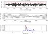 |
Fig. 2 Upper panel: full light curve of the star KIC 1163579 from quarters Q1–Q14. Middle panel: zoom into the above light curve. Periodicity and the existence of a second period is clearly visible, revealed by the double-dip structure around 550 days. Lower panel: periodogram of the full light curve. Significant peaks are marked in red, other peaks in the range of P1 ± 30% (indicated by the dashed blue lines) are marked in blue. |
The second point is the more interesting one because a higher frequency resolution offers the detection of individual peaks lying much closer than in the periodograms of the individual quarters. Thus, the frequency resolution is crucial for the detection of small values of differential rotation!
To achieve an almost continuous time series of each star we chose the easiest way to concatenate consecutive quarters by dividing the light curves of each quarter by its median and subtracting unity. Data outliers were removed as described in García et al. (2011). Light curves exhibiting low-frequency trends, i.e., increasing or decreasing behavior over the full 90 days window, were considered as not properly reduced by the PDC-MAP pipeline, and therefore discarded.
The method we apply to the full time series slightly differs from the previously used sine fit approach. We only compute one Lomb-Scargle periodogram of the whole time series. Owing to the increased amount of data each light curve was binned to six hours cadences to save computation time. This sampling still enables us to detect short periods down to half a day according to the Nyquist frequency fNyq ≈ 2 d-1. We identify the twenty highest peaks and search for periods within the limits 0.5 d ≤ P1 ≤ 60 d. Furthermore, we force a lower peak height limit of h1> 0.10 to get some significance for P1, and check for alias periods according to Eqs. (3) and (4).
An important point to make is that we do not over-sample the periodogram, in contrast to previous work (Reinhold et al. 2013). For the analysis of individual quarters oversampling was necessary because many cases only revealed a single broadened peak, rather than two or more distinct peaks. Therefore, a fine frequency sampling was necessary to subtract the correct period in the prewhitening to be able to detect more than one period. Owing to the much higher frequency resolution here, the periodogram is able to reveal individual peaks.
In the following section we try to assign a significance to individual peaks. The goal is to find out which peaks really carry information about different spot rotation periods, and which are related to spurious detections and/or stochastic effects, e.g., emerging and waning active regions.
3.2.1. Identification of significant peaks
Analogous to Eq. (5) we search for periods Pk within 30% of P1. We sort the peak heights in descending order according to h1>h2>... and compute the so-called peak height ratio (PHR) hk/hk + 1. This method is illustrated based on the example star KIC 1163579 in Fig. 3. The idea is to detect peaks with comparable heights, and to see where the peak height drops to a significantly lower value from one peak to the other. Hence, we compute the median of the PHR and search for the maximum deviation from this value. The related index k = kmax yields the number of significant peaks. In Fig. 3 the median is shown as solid red line, and the dashed red lines indicate the ± 1σ region. For this example, it is evident that for kmax = 3 the PHR is at maximum, which means that the peak height of P3 is much higher than that of P4, compared to all peak heights within P1 ± 30%. All periods Pk with k ≤ kmax are considered as significant, the others are discarded. The lower panel of Fig. 2 shows the periodogram of the active star KIC 1163579 with the significant peaks found by this method marked in red.
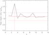 |
Fig. 3 The peak height ratio (PHR) hk/hk + 1 versus peak number k of the periodogram from Fig. 2. The solid red line shows the median PHR, and the dashed red lines mark the ± 1σ levels. At k = 3 the deviation from the median is at maximum, meaning that three significant peaks were found by this method. These are marked by red asterisks in Fig. 2. |
3.3. Analysis of segments of the full time series
This section contains another approach we used to extract information about different periods in the data. The primary peak in the periodogram of the full time series represents the best sine fit period over the full observing time. This period must be interpreted as an average rotation period because it fits certain parts of the light curve better than others. Adjacent peaks with less power are also needed to properly fit the data, and these periods may be more visible in certain segments than in the full light curve.
Minor peaks adjacent to P1 (e.g., peaks marked by blue asterisks in the lower panel of Fig. 2) result from various phenomena: differential rotation, spot evolution, and data reduction. Differentiating between these effects is almost impossible, but we assume that DR is the dominating effect in most cases. Spot evolution might be the strongest contributor of spurious detections of DR, where multiple peaks cannot be associated with spots rotating at different latitudes. Analyzing different segments thus becomes important, since the evolution of individual spots does not occur continuously in time, but may affect certain parts of the full light curve stronger than others. Another problem might be caused by stitching together individual quarters, where the end of one quarter and the beginning of the consecutive one do not agree with the overall variability pattern. This problem is intrinsic to the PDC-MAP pipeline, which was designed to remove instrumental effects from individual quarters, and not to conserve the overall variability pattern over the total observing time.
To overcome these effects we analyze segments with different lengths of the full light curve, aiming to detect periods that are stable over different timescales. In the following, segments are defined as concatenated quarters, starting with data from Q1−Q2, and adding the subsequent quarter in the next step, i.e., the second segment contains data from Q1–Q3, and so on, with the last segment being the full light curve Q1−Q14. We compute the periodogram of each segment5, interpolate it onto the frequency grid of the periodogram of the full light curve6, and add up the logarithmic powers of all segments. This leads to extremely clear periodograms, likely canceling spurious detections.
Figure 4 shows periodograms of the defined segments of the star KIC 1163579, clearly revealing multiple periods between 5−6 days in all segments. The main period crystallizes out around 5.4 days. Each periodogram reveals a period around 6.1 days, which was also found in the periodogram of the full time series (see Fig. 2), but was not considered as a significant period by our method. Thus, the measured value of DR might be largely underestimated in this case. To account for such periods with minor power, we sum up the logarithmic power of all segments, which is shown in the upper panel of Fig. 5. The main power is visible around P1 = 5.4 days, and also the first and second harmonic being the half and third of this period. In certain cases it occurs that the first harmonic, P1/ 2, has the second highest or even the highest power in the periodogram. Since we are interested in periods adjacent to P1 we subtract a fourth order polynomial (solid blue line in Fig. 5), and exponentiate the difference, which is shown in the lower panel of Fig. 5. This procedure leads to extremely clear periodograms. Periods lying within ± 30% of P1 with powers > 0.5 h1 are considered as significant. The dashed red line indicates the arbitrarily chosen significance limit. The period around 6.1 days survives this procedure, and will contribute to the DR measure in Sect. 4.2. Results combining our three different approaches are presented in the following section.
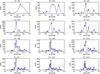 |
Fig. 4 Periodograms of the segments of KIC 1163579. Periodicity is clearly visible between 4.5−6.5 days. The location of the main peak around 5.4 days does not change much, whereas the number of minor peaks increases towards longer segments, owing to the higher frequency resolution. |
4. Results
We present rotation periods of more than 18 500 stars using the different approaches from Sects. 3.1–3.3. Based on these periods we search for differential rotation in Sect. 4.2. Mean rotation periods together with their uncertainties are used to infer stellar ages through different gyrochronology relations in Sect. 4.3. Finally, Sect. 4.4 is dedicated to a small fraction of stars exhibiting rotation periods very stable in time.
4.1. Rotation periods
In Fig. 6 we present the mean rotation period ⟨ P1 ⟩, averaged over the quarters Q1−Q14, versus color (B−V)0. The black dots show previous measurements from Reinhold et al. (2013), only using Q3 data. Green dots mark the 18 691 so-called good stars (see Sect. 3.1), and the 454 red and 625 blue dots indicate very stable rotators, which are discussed separately in Sect. 4.4. The dashed blue lines show isochrones from Barnes (2007) and the blue star marks the position of the Sun. Around (B−V)0 = 0.4 rotational braking due to magnetized winds becomes efficient. The 4500 Myr isochrone acts as an upper envelope to our measurements up to (B−V)0 ≃ 1.0. Coeval stars redder than (B−V)0 = 1.0 with supposably longer periods are missing due to the limited quarter length of ~90 days. A lower envelope to the rotation period distribution is given by the 200 Myr isochrone. Stars below this curve are either younger than 200 Myr, or are not suitable for the use of gyrochronology. The latter is also true for stars bluer than (B−V)0 = 0.4 (see Sect. 4.3.1). A second group of stars immediately leaps to the eye with short periods between 0.5–2 days and (B−V)0< 0.4. Most of these stars exhibit periods very stable in time, which we discuss separately in Sect. 4.4. Comparing the black and green dots it is evident that the period measurements have been considerably improved by incorporating more data.
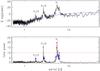 |
Fig. 5 Upper panel: summed up logarithmic powers of the periodograms of the individual segments from Fig. 4. The solid blue curve shows a fourth order polynomial fit. Lower panel: exponential power of the upper panel with the polynomial fit subtracted. Peaks above the arbitrarily chosen significance limit of 0.5 h1 (dashed red line) are considered as significant, and used as a measure of DR in the following. In this picture the harmonics (P1/ 2 and P1/ 3) are also more pronounced. |
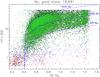 |
Fig. 6 Mean rotation periods ⟨ P1 ⟩ averaged over the quarters Q1–Q14 plotted against color (B−V)0. Previous measurements (Reinhold et al. 2013) only using Q3 data are shown in black, good measurements surviving the criteria described in Sect. 3.1 are shown in green. Red and blue dots show stars with periods very stable in time, which are discussed separately in Sect. 4.4. The dashed blue lines show isochrones from Barnes (2007), and the blue star marks the position of the Sun. |
For the three different approaches (Sects. 3.1–3.3) we compared our measurements to the state-of-the-art rotation periods from McQuillan et al. (2014) in Fig. 7. In general, all methods show very good agreement. In each panel the dashed red line shows the one-to-one period ratio, and the upper and lower dashed blue lines indicate the 2:1 and 1:2 period ratios, respectively. The left panel shows average periods from the quarters Q1−Q14, using the green, red, and blue dots from Fig. 6. We find 17 674 stars matching the two samples; 98.9% of these stars lie within 10% of those from McQuillan et al. (2014). A small fraction of 0.5% alias periods was found. The middle panel shows rotation periods derived from the analysis of the full light curve. 15 082 stars match, 97.4% do not differ by more than 10%, and 1.4% alias periods were found. The right panel shows measurements from the individual segments. 16 443 stars match, 96.0% within 10%, and 2.3% alias periods were detected.
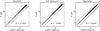 |
Fig. 7 Comparison of rotation periods P1 to the results of McQuillan et al. (2014) using different methods. The dashed red line denotes the 1:1 ratio, and the upper and lower dashed blue lines indicate the 2:1 and 1:2 period ratios, respectively. For each method the number of stars matching all criteria is given in the lower right corner of each panel. |
Combined period measurements from the methods above are shown in Fig. 8. We computed the median of the periods P1 derived from each method, allowing for a median absolute deviation (MAD) of one day for periods shorter than twenty days, and a MAD of two days for longer periods. In total, we find 18 599 stars matching with the sample of McQuillan et al. (2014). 97.6% of the periods lie within 10% of each other. In contrast to McQuillan et al. (2014) our sample contains stars hotter than 6500 K, and also a few stars which do not belong to their periodic sample. Since we are searching for DR in the following section, we do not restrict our sample to stars matching with McQuillan et al. (2014), but consider all stars with measured period P1 within the above MAD limits, additionally satisfying log g> 3.5 and Rvar> 0.3%.
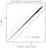 |
Fig. 8 Rotation period measurements combining the three different approaches from Fig. 7, and comparing them to AutoACF periods from McQuillan et al. (2014). |
4.2. Differential rotation
As shown in the previous section, rotation periods can be detected in a straightforward way by picking the highest periodogram peak and applying certain selection criteria. The situation is different when searching for differential rotation, acting as a perturbation to the main rotation period. We usually interpret the detection of a second period in the periodogram analysis as an indication of DR. Unfortunately, each method from Sects. 3.1–3.3 yields different results. For a certain star it occurs that one method returns a second period, whereas the other one does not. Even if all three methods yield a second period for a certain star, the periods found can differ a lot, depending on the different selection criteria and the frequency resolution. For that reason we define mean values for the DR of a certain star in the following.
We pick the minimum and maximum of the set of significant periods, individually for Sects. 3.2 and 3.3. If both methods yield a minimum and maximum period for a certain star, we compute the mean value, and call these periods Pmin and Pmax, respectively. We refrain from calculating minimum and maximum periods from individual quarter measurements owing to their lower frequency resolution. Thus, we define the relative and absolute horizontal shear α: = (Pmax−Pmin) /Pmax and dΩ: = 2π (1 /Pmin−1 /Pmax), respectively, as a measure of DR. In the following, we show how these two quantities correlate with rotation period and effective temperature. We only consider stars exhibiting a variability range Rvar> 0.3%, which was defined as a lower activity limit in Reinhold et al. (2013).
Figure 9 shows the relative shear α as a function of the minimum period Pmin. For stars cooler than 6700 K we find that α increases with rotation period. A contrary behavior is found for hot stars (Teff> 6700 K) populating the upper left corner (α> 0.02 and Pmin< 2 d). These short period stars spread a wide range of α, and clearly do not follow the overall trend. We suggest that multiple period measurements in these stars might actually be due to pulsations or rapid spot evolution, and should not be interpreted as DR. Owing to magnetic braking, cool stars exhibit longer periods, on average, thus populating the upper right part of Fig. 9. In the lower left corner (α< 0.01 and Pmin< 3 d) a mixture of all temperatures is found, indicating young fast rotating stars. Again, we warn the reader that these small α values can also be mis-classified as spot evolution. The dashed blue area shows theoretical predictions from Küker & Rüdiger (2011) for models with 0.3 M⊙ (bottom) to 1.1 M⊙ (top). These simulations agree well with our observations of relative shear increasing with rotation period. Furthermore, the hot stars are not covered by the model predictions, supporting our conclusion above. Almost 78% of the fast rotators (Pmin< 2 d) exhibit rotation periods very stable in time. These very stable periods are considered separately in Sect. 4.4.
We compared our findings to previous measurements from Hall (1991) who also found an increase of the relative shear with rotation period. The dash-dotted and dashed black lines show linear fits to our measurements in log-log space yielding a relation  with c = 0.71 discarding the hot stars (blue data points) and c = 0.55 using all data points, respectively. The first value is consistent with the result from Hall (1991) who found c = 0.79 ± 0.06.
We also compared our results to measurements from Donahue et al. (1996). These authors found a relation between the mean rotation period ⟨P⟩ and the observed period spread ΔP according to ΔP ∝ ⟨P⟩ 1.3 ± 0.1. Keeping in mind that α ∝ ΔP/ ⟨P⟩, we find ΔP ∝ ⟨P⟩ c + 1 = ⟨P⟩ 1.71. This value is slightly bigger than the value of 1.3 found by Donahue et al. (1996), regardless of whether discarding or keeping hot stars. The discrepancy might be explained by the fact that these authors only considered FGK stars, whereas we also incorporate M stars in our sample, usually exhibiting large values of α.
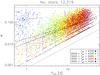 |
Fig. 9 Minimum period Pmin versus relative differential rotation α. The colors represent different temperature bins, the dotted black lines marks our detection limits. The dashed blue area shows theoretical predictions from Küker & Rüdiger (2011) for models with 0.3 M⊙ (bottom) to 1.1 M⊙ (top). We find that α increases with rotation period for stars cooler than 6700 K. The black lines show linear fits to our measurements, discarding stars hotter than 6700 K (dash-dotted line) and using all data points (dashed line), respectively. |
Figure 10 shows the dependence of the relative shear on effective temperature for a subset of stars satisfying 2 d <P1< 3 d. The dash-dotted red and dashed orange curves show theoretical predictions from Küker & Rüdiger (2011) using a model with an equatorial rotation period of 2.5 days. Between 3000–6000 K the red curve matches the observations quite well, although the slope of the curve is too small. Stars hotter than 6000 K are well represented by the slope of the orange curve, although our observations are offset towards higher temperatures. We are using revised temperatures from Huber et al. (2014), being on average 200 K hotter for hot stars and 200 K cooler for cool stars, compared to previous temperatures from the KIC, which might explain this offset. We do not want to emphasize the comparison of our observations to the models because we do not find a clear trend when using all rotation periods. This is consistent with previous work (Reinhold et al. 2013), where only a shallow trend of α towards cooler stars has been found. We now interpret this shallow increase of α as a consequence of the increase of rotation period towards cooler stars.
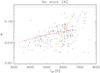 |
Fig. 10 Teff versus α for stars satisfying 2 d <P1< 3 d. The dash-dotted red and dashed orange curve show models from Küker & Rüdiger (2011). The dotted black line marks the upper limit of α. No distinct correlation between Teff and α was found. |
In Fig. 11 we plot the absolute shear dΩ against rotation period Pmin. We find that dΩ does not strongly depend on rotation period over a wide period range. Towards fast rotators with periods of a few days, the absolute shear increases, although showing large scatter. Again, we find that the upper left corner is populated by hot stars (see Fig. 9), which are clearly separated from the overall trend. Again, we warn the reader that these large dΩ values might not be associated with strong surface shear, but with different pulsation frequencies or rapid spot evolution. The dashed blue area shows theoretical models from Fig. 3 in Küker & Rüdiger (2011) with 0.3 M⊙ (bottom) to 1.1 M⊙ (top), which cover most of our measurements, but do not touch the hot stars with dΩ > 0.1 rad d-1.
Equivalent to Fig. 9 we applied a linear fit to our measurements yielding dΩ ∝ ⟨P⟩ c ∝ ⟨Ω⟩ − c with c = −0.29 discarding hot stars (dash-dotted line) and c = −0.45 using all data points (dashed line) in Fig. 11, respectively. We find good agreement with measurements from Barnes et al. (2005) claiming dΩ ∝ ⟨Ω⟩ 0.15 ± 0.10, confirming the weak dependence of the absolute shear on the rotation rate.
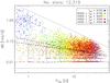 |
Fig. 11 Minimum period Pmin versus absolute differential rotation dΩ. The colors represent different temperature bins, the dotted black lines mark our detection limits. The dashed blue area shows theoretical predictions from Küker & Rüdiger (2011). We found that dΩ is almost independent of rotation period over a wide period range, but slightly increases towards short periods. Stars hotter than 6700 K do not follow the overall trend. The black lines show linear fits to our measurements, discarding stars hotter than 6700 K (dash-dotted line) and using all data points (dashed line), respectively. |
The dependence of the absolute shear on effective temperature is shown in Fig. 12. Our measurements (gray dots) suggest the existence of two distinct regions with different behavior of dΩ. From 3500−6000 K the absolute shear slightly increases showing weak dependence on temperature. Above 6000 K dΩ steeply increases with temperature, although showing large scatter. Data collected by Barnes et al. (2005) is plotted as purple diamonds, and the corresponding fit from Collier Cameron (2007) is shown as dotted purple line. These authors predicted a very strong temperature dependence (d ), which is not supported by our measurements. Light blue diamonds show measurements7 from Ammler-von Eiff & Reiners (2012) that are in good agreement with our findings. Theoretical predictions from Küker & Rüdiger (2011) are shown as dash-dotted red and dashed orange curve. These authors found no sufficient match when fitting their results with one polynomial over the whole temperature range. Therefore, they suggested a different behavior of dΩ above and below ~6000 K. Their curves fit remarkably well with the mean values of our measurements, shown as thick blue line. The matching gets even better when using the old KIC temperatures, rather than the new values from Huber et al. (2014), which are 200 K hotter (cooler) for the hot (cool) stars, on average. The model from Küker & Rüdiger (2011) is drawn from a star rotating with an equatorial period of Peq = 2.5 d. Our observations contain various rotation periods, which might explain the spread. In Sect. 5 we discuss reasons for the observed spread, including cases with multiple periods mis-interpreted as DR. The measured values of Pmin, Pmax, α, and dΩ are collected in Table 2. The measured period differences are used as uncertainties for determining gyrochronology ages in the next section.
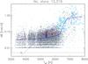 |
Fig. 12 Effective temperature Teff versus absolute shear dΩ summarizing different measurements: purple diamonds were taken from Barnes et al. (2005), the dotted purple curve from Collier Cameron (2007). Light blue diamonds show measurements from Ammler-von Eiff & Reiners (2012). Our measurements are shown as gray dots. The thick blue line represents the weighted mean of our measurements for 250 K temperature bins. The dash-dotted red line and the dashed orange line show theoretical predictions from Küker & Rüdiger (2011). The dotted black line represents our detection limit, and the red star marks the position of the Sun. We find that dΩ shows weak dependence on effective temperature between 3300–6200 K. Above 6200 K dΩ strongly increases showing large scatter. |
4.3. Stellar ages
4.3.1. Gyrochronology
After measuring mean rotation periods P and period variations ΔP for two-thirds of the sample, we calculate stellar ages t along with their uncertainties Δt using different gyrochronology relations (Barnes 2007; Mamajek & Hillenbrand 2008; Meibom et al. 2009), hereafter abbreviated as B07, MH08, and MMS09, respectively. Ages are calculated according to Eq. (3) in Barnes (2007), ![Mathematical equation: \begin{equation} \label{age_eq} \log t = \frac{1}{n}[\log P - \log a - b\,\log X], \end{equation}](/articles/aa/full_html/2015/11/aa26216-15/aa26216-15-eq107.png) (6)with X: = (B−V)0−c and different fit parameters a,b,c,n (see Table 3). Colors (B−V)0 are obtained by converting g−r8 to (B−V) color using the relation from Jester et al. (2005) and subtracting the excess B−V reddening E(B−V)8.
(6)with X: = (B−V)0−c and different fit parameters a,b,c,n (see Table 3). Colors (B−V)0 are obtained by converting g−r8 to (B−V) color using the relation from Jester et al. (2005) and subtracting the excess B−V reddening E(B−V)8.
Fit parameters and period and color constraints used in the different gyrochronology relations.
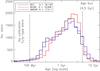 |
Fig. 13 Stellar age distributions derived from different gyrochronology relations: Barnes (2007), Mamajek & Hillenbrand (2008), Meibom et al. (2009). Their calibration ranges are given in Table 3. Stars with derived ages younger than 100 Myr (left of the dashed black line) should be treated with caution. |
Age uncertainties are calculated according to Eq. (10) in Barnes (2007), 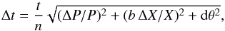 (7)with ΔP: = (Pmax−Pmin)/2 being the uncertainty of the mean period P, and ΔX being the (B−V) difference between the conversion from Jester et al. (2005) and Bilir et al. (2005). Frequently, this difference is rather small, and no uncertainties for the SDSS g−r colors were found in the literature. Thus, we set a minimum uncertainty of ± 0.01 mag to the (B−V) colors with smaller uncertainties. The term dθ2 contains uncertainties of the fit parameters from Table 3 (compare Eq. (10) in Barnes 2007). If DR was detected the period uncertainty dominates the age uncertainty, especially for the slowly rotating stars with ΔP of a few days.
Rotation periods, (B−V)0 colors, and gyrochronology ages using different calibrations.
Distributions of the derived ages are shown in Fig. 13. For our stellar ages sample we retain stars that are not contained in the McQuillan et al. (2014) sample, but remove those with stable rotation periods (see Sect. 4.4). The latter might not have spun down to the I-sequence yet (see Barnes 2003 for terminology), or their rotation might be controlled by non-eclipsing companions. Additionally, we tighten our limit of the surface gravity to log g ≥ 4.2 to ensure that gyrochronology relations are only applied to dwarf stars.
The MH08 and MMS09 distributions contain fewer stars than the B07 distribution owing to the different color ranges (see Table 3). The color and period constraints are needed to ensure that our field star sample obeys the same (or at least a similar) dependence of rotation period on color and age as the cluster stars used for calibration. The derived ages are collected in Table 4, and their reliability is discussed in more detail in Sect. 5.
Derived ages younger than 100 Myr should be treated with caution. These stars cover the full (B−V)0 range, but mostly exhibit rotation periods less than five days. They likely have not yet converged to the I-sequence, and thus are not suitable for applying gyrochronology relations. The right edge of the distribution with derived ages older than 10 Gyr can also not be trusted since roughly half of the stars exhibit ages older than the universe. These values result from a combination of long rotation periods (P> 20) days and effective temperatures > 5500 K, with either or both of them being erroneous.
Using the B07 distribution 17 623 stars possess ages between 100 Myr and 10 Gyr. Of these stars, 90.7% are younger than 4 Gyr, in good agreement with Matt et al. (2015) estimating ~95% comparing the sample from McQuillan et al. (2014) to model predictions. Less than 0.62% of the derived ages are greater than 10 Gyr, and less than 2.2% of the B07 stars lie in the critical calibration region younger than 100 Myr, providing some confidence in the derived age distribution.
4.3.2. Activity-age relation
Inspired by Fig. 8 in Soderblom et al. (1991) we are interested in deriving a similar activity-age relation. Unfortunately, spectra of Kepler stars are lacking, so we cannot compare the derived ages to the established chromospheric activity measure . Nevertheless, the variability range Rvar can be used as an activity indicator in a statistical sense. Using the B07 distribution we plot the age against the variability range in Fig. 14, which was inspired by Fig. 4 in McQuillan et al. (2014). The ages were derived only using periods lying closer than 10% to periods found by McQuillan et al. (2014). From the upper left to the lower right, the temperature increases from 3200–6200 K in 500 K intervals. The upper panels (3200–4700 K) shows a bimodality of the age distribution, which vanishes for hotter stars. This incident was first detected by McQuillan et al. (2013a) for the Kepler M dwarf periods, and confirmed later that the bimodality extends to hotter stars (Reinhold et al. 2013; McQuillan et al. 2014). Moreover, the gap separating the two peaks shifts towards younger stars with increasing temperature, starting at ~800 Myr for the coolest stars (3200–3700 K), and descends to 500 Myr for stars between 4200–4700 K. For each temperature bin the point distribution shows that the variability range decreases with age, although each distribution exhibits large scatter in Rvar. This general behavior is expected from the observation that young stars are, on average, more active than old ones. In each panel two point clouds are visible. Thus, we separated the two clouds into a so-called young and old sample. To guide the eye we empirically drew a dashed red line between the two samples, with increasing slope towards hotter temperatures, and varying offset in each panel. Stars lying below (above) the dashed red line belong to the young (old) sample, respectively. There are other ways of defining a young and an old sample, e.g., using the horizontal dashed black line separating the two peaks of the bimodal distribution, but we wanted to emphasize the correlation between activity and age. We were curious if the parameters of these distinct samples substantially differ. Thus, we plotted histograms of common stellar parameters such as log g, FeH, brightness, and so on. Unfortunately, we found no major difference in the parameters that could explain the evidence of the two point clouds. However, we found a correlation between the ages shown and the corresponding peak heights of the primary periodogram peaks. The peak heights of the young sample were, on average, higher than the peaks of the old sample. We interpret this result in terms of young stars being more active. Hence, their light curves are more sinusoidal because they suffer less by DR, spot evolution, or instrumental flaws, all effects disrupting the light curve shape.
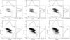 |
Fig. 14 Gyrochronology ages plotted against the variability range for 500 K temperature bins between 3200–6200 K. The age distribution shows a bimodality between 3200–4700 K, which vanishes for hotter stars. The variability range Rvar decreases with age, becoming more emphasized towards hotter stars (increasing slope of dashed red line). |
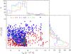 |
Fig. 15 Stars with super-stable periods (MAD(P1) < 0.001 d, red), and very stable periods (0.001 < MAD(P1) < 0.01 d, blue). The inner green dots denote stars where a second period was found. The temperature and period distributions are shown in the top and right panel, respectively. |
4.4. Extremely stable periods
From the analysis of the individual quarters we found periods P1,Q that are extremely stable in time. These stars have previously been shown in Fig. 6, and are analyzed in more detail here. To quantify their temporal stability we computed the median absolute deviation  , and categorized two groups of stable periodic stars: super-stable stars with MAD(P1) < 0.001 d, and very stable stars satisfying 0.001 < MAD(P1) < 0.01 d. These stars are flagged in the last column of Table 4. We emphasize that these periods are stable over more than three years of observation!
Figure 15 shows the periods and effective temperatures of both groups. Super-stable and very stable periods are shown as red and blue dots, respectively. Inner green dots denote stars where a second period was found. The temperature and period distributions are shown in the upper and right panel, respectively. The period distribution shows that most of the super-stable stars exhibit short periods less than one day, with a mean period of ⟨ P1 ⟩ = 0.95 d. The very stable stars extend to longer periods up to ~12 d, with a mean of ⟨ P1 ⟩ = 1.90 d. Stars with a second period were found in both groups, but only between 0.5−4.2 days. The temperature distribution shows that the vast majority of both groups exhibit temperatures less than 8000 K, with a mean of ~6800 K for the super-stable stars. The very stable stars are, on average, 700 K cooler. Both distributions populate the full temperature range, but stars with a second period were almost exclusively found below 8000 K. Between 8000−10 000 K a dearth of second period stars was found, and only a few second period stars were found above 10 000 K.
There exist two general explanations for the observed stable periodic variability. One possible explanation are stellar pulsations, which are known to be very stable in time. The other process serving as an astronomical clock is synchronization by a companion. We calculated the MAD(P1) with the intention of disentangling these two processes. In the period regime of 0.5–4 days δ Scuti, γ Dor, and their hybrid pulsators of these are expected. The boundaries of the so-called instability strip (i.e., the region in the Hertzsprung–Russell diagram populated by these pulsators) is expected roughly between 6500–8800 K. Surprisingly, most of the stable stars exhibit temperatures less than 8000 K. A fraction of them might actually be γ Dor stars between 6500–7000 K, but there is no pulsation mechanism able to produce such stable periods in the cool stars regime. Stable periods above 8000 K are likely caused by pulsations because spots are not necessarily expected for such hot stars. Thus, we favor the conclusion that the periodicity of stars cooler than 6500 K is caused by spots on the stellar surface stabilized by non-eclipsing companions, either due to interactions with another star or a close-in planet. Moreover, this hypothesis is supported by the observation that stars with multiple periods (indicative for DR) were mostly found below 8000 K.
5. Discussion
5.1. Rotation
-
We measured rotation periods for a statistically meaningfulensemble of stars. In total, more than 18 500rotation periods we derived using different approaches, allrevealing very good agreement with the results from McQuillanet al. (2014).
-
As discussed in the previous section, we found 1079 periods extremely stable in time, with a median absolute deviation less than 0.01 d. For stars cooler than 6500 K binarity is the favored explanation. In our total sample (see Table 4) we have 5124 stars with P1< 10 d and Teff< 6500 K. 573 of these stars exhibit stable periods, which corresponds to a percentage of ~11.2%. van Saders & Pinsonneault (2013) state that tidally synchronized binaries are fast rotators with periods less than 10 days and that they contaminate the field with 4%, compared to 11% in the Hyades (Duquennoy & Mayor 1991). Our rate is almost three times higher than the expected percentage of tidally locked field star binaries, but comparable to the expected percentage in the Hyades. One possible explanation may be the existence of non-transiting planets, which are able to decrease the angular momentum loss rate due to magnetized winds (Cohen et al. 2010). Additionally, pulsating stars cooler than 6500 K might contribute to this rate. Other explanations for stable rotation might be different dynamos. Brown (2014) suggests the so-called Metastable Dynamo, where stars are born rapidly rotating with weak coupling to the wind. Other dynamo mechanisms might generate strong magnetic fields leading to long spot lifetimes.
5.2. Differential rotation
-
Exact values of α and dΩ are hard to determine, and depend on the particular threshold used. Depending on which periods are selected as Pmin and Pmax, the absolute values of α and dΩ can differ a lot. Nevertheless, each method from Sects. 3.1–3.3 produces the same correlations for α and dΩ with temperature and period. Combined measurements from the different approaches, as described at the beginning of Sect. 4.2, were used to provide average values of Pmin and Pmax. As discussed by the example of Fig. 12 the observed spread in dΩ can only partially be explained by theory. Collier Cameron & Donati (2002) and Donati et al. (2003) found a large spread in dΩ ranging from 0.046−0.091 rad d-1 for the active star AB Dor. Evolving spot configurations might be an explanation. Hence, all measurements here should be interpreted in a statistical way.
-
Although the derived values are method dependent, the statistical averages are not. Our results are in good agreement with previous measurements (Hall 1991; Donahue et al. 1996) and theoretical predictions (Küker & Rüdiger 2011).
-
Simulations of spotted stars exhibiting rapid spot evolution are able to generate beat-shaped light curves, multiple periodogram peaks, and therefore able to mimic DR. This interpretation was not considered so far. We think that spot evolution may play a role, but we have no way to discriminate between these two phenomena.
5.3. Stellar ages
-
All gyrochronology relations have been calibrated byground-based observations of open clusters and Mount Wilsonstars. The stars used in the different calibrations exhibit differentperiod and color ranges. Age calibration was performed using theSun as an age anchor. Thus, the relations are not tested for starsolder than the Sun. Applying these relations to stars with a widerperiod and color range might lead to less accurate ages.
-
Gyrochronology ages are most reliable between 500−2500 Myr. Depending on their braking efficiency some stars younger than 500 Myr may not have converged to the I-sequence yet. Thus, their periods may not be suitable for the use of gyrochronology. The calibration becomes even worse for stars with derived ages less than 100 Myr. Such stars might belong to the C-sequence, obeying a physically different behavior. We do not trust derived ages younger than 100 Myr or older than 10 Gyr.
-
Subgiants and main sequence stars obey a different rotation-age relationship (García et al. 2014). In this study we attempt to exclude evolved stars by setting a lower limit to the surface gravity of log g ≥ 4.2. Unfortunately, Kepler does not provide stellar luminosity classification, so our sample might be contaminated by subgiants. Contamination might be as large as 35% for field stars as pointed out by van Saders & Pinsonneault (2013).
-
The existence of the two point clouds in Fig. 14 for stars with 3200 <Teff< 4700 K is a matter of debate. McQuillan et al. (2014) suggested that the bimodality of the age distribution can be understood in terms of two distinct star formation events in the solar neighborhood. Stellar ages are correlated with the variability range in the sense that young stars are more active, on average. Interestingly, this trend becomes more distinct towards hotter stars, as indicated by the dashed red line in Fig. 14, which lacks an explanation so far.
-
A comparison of gyrochronology and asteroseismology ages is challenging. Much progress was recently made (see, e.g., Angus et al. 2015). Most rotation period and asteroseismology samples do not overlap because strong activity, essential for achieving spot rotation periods, damps mode excitation (Chaplin et al. 2011). Furthermore, Kepler lacks bright stars, which are needed for asteroseismology. Upcoming missions will hopefully change this unpleasant situation in the near future.
6. Summary
We reanalyzed the sample of 24 124 stars from Reinhold et al. (2013) using Q1–Q14 data. Good agreement was found with previous rotation periods and measurements from McQuillan et al. (2014). We searched for deviations from the mean rotation period using the Lomb-Scargle periodogram in different approaches, aiming to detect multiple significant periods, and assigning them to surface differential rotation. The general trends of the DR with period and temperature, observed in Reinhold et al. (2013), could all be confirmed although individual measurements of α and dΩ may differ due to the different frequency resolution of the full time series and the 90-days time base of a single quarter. In general, the new measurements are in very good agreement with previous observations (Hall 1991; Donahue et al. 1996) and theoretical predictions (Küker & Rüdiger 2011). Stellar ages were derived from gyrochronology relations provided by different authors, with uncertainties that are dominated by the period spread. A bimodal age distribution was found between 3200–4700 K, vanishing for hotter star. The derived ages show a correlation with the variability range serving as an activity indicator. Furthermore, we found 1079 stars exhibiting a very stable period, with a median absolute deviation less than 0.01 d. The almost constant periods of the hot stars may be explained by pulsations, whereas the stability of the cooler star (Teff< 6500 K) may be explained with synchronization of the orbital period of a non-eclipsing companion.
In the following, the variability range Rvar is meant to be the median of the periods P1,Q for the quarters Q1–Q14.
For the individual segments we use the normalization from Eq. (22) in Zechmeister & Kürster (2009).
This is necessary because periodograms of different segments possess a different frequency resolution.
The values were taken from Table 2 in Ammler-von Eiff & Reiners (2012) assuming an inclination of 90°.
Taken from the Kepler Input Catalog (KIC).
Acknowledgments
We would like to thank the referee, Sydney Barnes, for providing very constructive suggestions, which led to significant improvements to the paper, especially to the differential rotation discussion. We acknowledge support from Deutsche Forschungsgemeinschaft Collaborative Research Center SFB-963 “Astrophysical Flow Instabilities and Turbulence” (Project A18).
References
- Affer, L., Micela, G., Favata, F., & Flaccomio, E. 2012, MNRAS, 424, 11 [NASA ADS] [CrossRef] [Google Scholar]
- Ammler-von Eiff, M., & Reiners, A. 2012, A&A, 542, A116 [NASA ADS] [CrossRef] [EDP Sciences] [Google Scholar]
- Angus, R., Aigrain, S., Foreman-Mackey, D., & McQuillan, A. 2015, MNRAS, 450, 1787 [NASA ADS] [CrossRef] [Google Scholar]
- Balona, L. A. 2014, MNRAS, 437, 1476 [NASA ADS] [CrossRef] [Google Scholar]
- Balona, L. A., Cunha, M. S., Kurtz, D. W., et al. 2011, MNRAS, 410, 517 [NASA ADS] [CrossRef] [Google Scholar]
- Barnes, S. A. 2003, ApJ, 586, 464 [NASA ADS] [CrossRef] [Google Scholar]
- Barnes, S. A. 2007, ApJ, 669, 1167 [NASA ADS] [CrossRef] [Google Scholar]
- Barnes, S. A. 2010, ApJ, 722, 222 [NASA ADS] [CrossRef] [Google Scholar]
- Barnes, J. R., Collier Cameron, A., Donati, J.-F., et al. 2005, MNRAS, 357, L1 [NASA ADS] [CrossRef] [MathSciNet] [Google Scholar]
- Basri, G., Walkowicz, L. M., Batalha, N., et al. 2010, ApJ, 713, L155 [NASA ADS] [CrossRef] [Google Scholar]
- Basri, G., Walkowicz, L. M., Batalha, N., et al. 2011, AJ, 141, 20 [NASA ADS] [CrossRef] [Google Scholar]
- Benkő, J. M., Kolenberg, K., Szabó, R., et al. 2010, MNRAS, 409, 1585 [NASA ADS] [CrossRef] [Google Scholar]
- Bilir, S., Karaali, S., & Tunçel, S. 2005, Astron. Nachr., 326, 321 [NASA ADS] [CrossRef] [Google Scholar]
- Brown, T. M. 2014, ApJ, 789, 101 [NASA ADS] [CrossRef] [Google Scholar]
- Chanamé, J., & Ramírez, I. 2012, ApJ, 746, 102 [NASA ADS] [CrossRef] [Google Scholar]
- Chaplin, W. J., Bedding, T. R., Bonanno, A., et al. 2011, ApJ, 732, L5 [Google Scholar]
- Chaplin, W. J., Basu, S., Huber, D., et al. 2014, ApJS, 210, 1 [NASA ADS] [CrossRef] [Google Scholar]
- Cohen, O., Drake, J. J., Kashyap, V. L., Sokolov, I. V., & Gombosi, T. I. 2010, ApJ, 723, L64 [NASA ADS] [CrossRef] [Google Scholar]
- Collier Cameron, A. 2007, Astron. Nachr., 328, 1030 [NASA ADS] [CrossRef] [Google Scholar]
- Collier Cameron, A., & Donati, J.-F. 2002, MNRAS, 329, L23 [NASA ADS] [CrossRef] [Google Scholar]
- Collier Cameron, A., Davidson, V. A., Hebb, L., et al. 2009, MNRAS, 400, 451 [NASA ADS] [CrossRef] [Google Scholar]
- Delorme, P., Collier Cameron, A., Hebb, L., et al. 2011, MNRAS, 413, 2218 [NASA ADS] [CrossRef] [Google Scholar]
- do Nascimento, Jr., J.-D., García, R. A., Mathur, S., et al. 2014, ApJ, 790, L23 [NASA ADS] [CrossRef] [Google Scholar]
- Donahue, R. A., Saar, S. H., & Baliunas, S. L. 1996, ApJ, 466, 384 [NASA ADS] [CrossRef] [Google Scholar]
- Donati, J.-F., Collier Cameron, A., & Petit, P. 2003, MNRAS, 345, 1187 [NASA ADS] [CrossRef] [Google Scholar]
- Doǧan, G., Metcalfe, T. S., Deheuvels, S., et al. 2013, ApJ, 763, 49 [NASA ADS] [CrossRef] [Google Scholar]
- Duquennoy, A., & Mayor, M. 1991, A&A, 248, 485 [NASA ADS] [Google Scholar]
- García, R. A., Hekker, S., Stello, D., et al. 2011, MNRAS, 414, L6 [NASA ADS] [CrossRef] [Google Scholar]
- García, R. A., Ceillier, T., Salabert, D., et al. 2014, A&A, 572, A34 [NASA ADS] [CrossRef] [EDP Sciences] [Google Scholar]
- Guggenberger, E., Kolenberg, K., Nemec, J. M., et al. 2012, MNRAS, 424, 649 [NASA ADS] [CrossRef] [Google Scholar]
- Hall, D. S. 1991, in The Sun and Cool Stars. Activity, Magnetism, Dynamos, eds. I. Tuominen, D. Moss, & G. Rüdiger (Berlin: Springer Verlag), IAU Colloq., 130, Lect. Notes Phys., 380, 353 [Google Scholar]
- Huber, D., Silva Aguirre, V., Matthews, J. M., et al. 2014, ApJS, 211, 2 [NASA ADS] [CrossRef] [Google Scholar]
- James, D. J., Barnes, S. A., Meibom, S., et al. 2010, A&A, 515, A100 [NASA ADS] [CrossRef] [EDP Sciences] [Google Scholar]
- Jester, S., Schneider, D. P., Richards, G. T., et al. 2005, AJ, 130, 873 [NASA ADS] [CrossRef] [Google Scholar]
- Kolenberg, K., Szabó, R., Kurtz, D. W., et al. 2010, ApJ, 713, L198 [NASA ADS] [CrossRef] [Google Scholar]
- Küker, M., & Rüdiger, G. 2011, Astron. Nachr., 332, 933 [NASA ADS] [CrossRef] [Google Scholar]
- Lampens, P., Tkachenko, A., Lehmann, H., et al. 2013, A&A, 549, A104 [NASA ADS] [CrossRef] [EDP Sciences] [Google Scholar]
- Lebreton, Y., & Goupil, M. J. 2014, A&A, 569, A21 [NASA ADS] [CrossRef] [EDP Sciences] [Google Scholar]
- Mamajek, E. E., & Hillenbrand, L. A. 2008, ApJ, 687, 1264 [NASA ADS] [CrossRef] [Google Scholar]
- Matt, S. P., Brun, A. S., Baraffe, I., Bouvier, J., & Chabrier, G. 2015, ApJ, 799, L23 [NASA ADS] [CrossRef] [Google Scholar]
- McQuillan, A., Aigrain, S., & Mazeh, T. 2013a, MNRAS, 432, 1203 [NASA ADS] [CrossRef] [MathSciNet] [Google Scholar]
- McQuillan, A., Mazeh, T., & Aigrain, S. 2013b, ApJ, 775, L11 [NASA ADS] [CrossRef] [Google Scholar]
- McQuillan, A., Mazeh, T., & Aigrain, S. 2014, ApJS, 211, 24 [NASA ADS] [CrossRef] [MathSciNet] [Google Scholar]
- Meibom, S., Mathieu, R. D., & Stassun, K. G. 2009, ApJ, 695, 679 [NASA ADS] [CrossRef] [Google Scholar]
- Meibom, S., Barnes, S. A., Latham, D. W., et al. 2011a, ApJ, 733, L9 [NASA ADS] [CrossRef] [Google Scholar]
- Meibom, S., Mathieu, R. D., Stassun, K. G., Liebesny, P., & Saar, S. H. 2011b, ApJ, 733, 115 [NASA ADS] [CrossRef] [Google Scholar]
- Meibom, S., Barnes, S. A., Platais, I., et al. 2015, Nature, 517, 589 [NASA ADS] [CrossRef] [PubMed] [Google Scholar]
- Molnár, L., Kolláth, Z., Szabó, R., et al. 2012, ApJ, 757, L13 [Google Scholar]
- Moskalik, P., Smolec, R., Kolenberg, K., et al. 2012 [arXiv:1208.4251] [Google Scholar]
- Nemec, J. M., Smolec, R., Benkő, J. M., et al. 2011, MNRAS, 417, 1022 [NASA ADS] [CrossRef] [Google Scholar]
- Nemec, J. M., Cohen, J. G., Ripepi, V., et al. 2013, ApJ, 773, 181 [NASA ADS] [CrossRef] [Google Scholar]
- Nielsen, M. B., Gizon, L., Schunker, H., & Karoff, C. 2013, A&A, 557, L10 [NASA ADS] [CrossRef] [EDP Sciences] [Google Scholar]
- Noyes, R. W., Hartmann, L. W., Baliunas, S. L., Duncan, D. K., & Vaughan, A. H. 1984, ApJ, 279, 763 [NASA ADS] [CrossRef] [Google Scholar]
- Pallavicini, R., Golub, L., Rosner, R., et al. 1981, ApJ, 248, 279 [NASA ADS] [CrossRef] [Google Scholar]
- Perryman, M. A. C., Brown, A. G. A., Lebreton, Y., et al. 1998, A&A, 331, 81 [NASA ADS] [Google Scholar]
- Pizzolato, N., Maggio, A., Micela, G., Sciortino, S., & Ventura, P. 2003, A&A, 397, 147 [NASA ADS] [CrossRef] [EDP Sciences] [Google Scholar]
- Reinhold, T., Reiners, A., & Basri, G. 2013, A&A, 560, A4 [NASA ADS] [CrossRef] [EDP Sciences] [Google Scholar]
- Skumanich, A. 1972, ApJ, 171, 565 [NASA ADS] [CrossRef] [Google Scholar]
- Smith, J. C., Stumpe, M. C., Van Cleve, J. E., et al. 2012, PASP, 124, 1000 [NASA ADS] [CrossRef] [Google Scholar]
- Soderblom, D. R. 2010, ARA&A, 48, 581 [NASA ADS] [CrossRef] [Google Scholar]
- Soderblom, D. R., Duncan, D. K., & Johnson, D. R. H. 1991, ApJ, 375, 722 [NASA ADS] [CrossRef] [Google Scholar]
- Stumpe, M. C., Smith, J. C., Van Cleve, J. E., et al. 2012, PASP, 124, 985 [NASA ADS] [CrossRef] [Google Scholar]
- Stumpe, M. C., Smith, J. C., Catanzarite, J. H., et al. 2014, PASP, 126, 100 [NASA ADS] [CrossRef] [Google Scholar]
- Szabó, R., Kolláth, Z., Molnár, L., et al. 2010, MNRAS, 409, 1244 [NASA ADS] [CrossRef] [Google Scholar]
- Tkachenko, A., Aerts, C., Yakushechkin, A., et al. 2013, A&A, 556, A52 [NASA ADS] [CrossRef] [EDP Sciences] [Google Scholar]
- Ulusoy, C., Stateva, I., Iliev, I. K., & Ulaş, B. 2014, New Astron., 30, 28 [NASA ADS] [CrossRef] [Google Scholar]
- Uytterhoeven, K., Moya, A., Grigahcène, A., et al. 2011, A&A, 534, A125 [NASA ADS] [CrossRef] [EDP Sciences] [Google Scholar]
- van Saders, J. L., & Pinsonneault, M. H. 2013, ApJ, 776, 67 [NASA ADS] [CrossRef] [Google Scholar]
- Vidotto, A. A., Gregory, S. G., Jardine, M., et al. 2014, MNRAS, 441, 2361 [NASA ADS] [CrossRef] [Google Scholar]
- Walkowicz, L. M., & Basri, G. S. 2013, MNRAS, 436, 1883 [NASA ADS] [CrossRef] [Google Scholar]
- Zechmeister, M., & Kürster, M. 2009, A&A, 496, 577 [NASA ADS] [CrossRef] [EDP Sciences] [Google Scholar]
All Tables
Fit parameters and period and color constraints used in the different gyrochronology relations.
Rotation periods, (B−V)0 colors, and gyrochronology ages using different calibrations.
All Figures
|
Fig. 1 Light curves (black) and sine fits (red) according to Eq. (2) of the star KIC 1163579 for all quarters Q1–Q14. Period measurements of this star are given in Table 1. |
| In the text | |
|
Fig. 2 Upper panel: full light curve of the star KIC 1163579 from quarters Q1–Q14. Middle panel: zoom into the above light curve. Periodicity and the existence of a second period is clearly visible, revealed by the double-dip structure around 550 days. Lower panel: periodogram of the full light curve. Significant peaks are marked in red, other peaks in the range of P1 ± 30% (indicated by the dashed blue lines) are marked in blue. |
| In the text | |
|
Fig. 3 The peak height ratio (PHR) hk/hk + 1 versus peak number k of the periodogram from Fig. 2. The solid red line shows the median PHR, and the dashed red lines mark the ± 1σ levels. At k = 3 the deviation from the median is at maximum, meaning that three significant peaks were found by this method. These are marked by red asterisks in Fig. 2. |
| In the text | |
|
Fig. 4 Periodograms of the segments of KIC 1163579. Periodicity is clearly visible between 4.5−6.5 days. The location of the main peak around 5.4 days does not change much, whereas the number of minor peaks increases towards longer segments, owing to the higher frequency resolution. |
| In the text | |
|
Fig. 5 Upper panel: summed up logarithmic powers of the periodograms of the individual segments from Fig. 4. The solid blue curve shows a fourth order polynomial fit. Lower panel: exponential power of the upper panel with the polynomial fit subtracted. Peaks above the arbitrarily chosen significance limit of 0.5 h1 (dashed red line) are considered as significant, and used as a measure of DR in the following. In this picture the harmonics (P1/ 2 and P1/ 3) are also more pronounced. |
| In the text | |
|
Fig. 6 Mean rotation periods ⟨ P1 ⟩ averaged over the quarters Q1–Q14 plotted against color (B−V)0. Previous measurements (Reinhold et al. 2013) only using Q3 data are shown in black, good measurements surviving the criteria described in Sect. 3.1 are shown in green. Red and blue dots show stars with periods very stable in time, which are discussed separately in Sect. 4.4. The dashed blue lines show isochrones from Barnes (2007), and the blue star marks the position of the Sun. |
| In the text | |
|
Fig. 7 Comparison of rotation periods P1 to the results of McQuillan et al. (2014) using different methods. The dashed red line denotes the 1:1 ratio, and the upper and lower dashed blue lines indicate the 2:1 and 1:2 period ratios, respectively. For each method the number of stars matching all criteria is given in the lower right corner of each panel. |
| In the text | |
|
Fig. 8 Rotation period measurements combining the three different approaches from Fig. 7, and comparing them to AutoACF periods from McQuillan et al. (2014). |
| In the text | |
|
Fig. 9 Minimum period Pmin versus relative differential rotation α. The colors represent different temperature bins, the dotted black lines marks our detection limits. The dashed blue area shows theoretical predictions from Küker & Rüdiger (2011) for models with 0.3 M⊙ (bottom) to 1.1 M⊙ (top). We find that α increases with rotation period for stars cooler than 6700 K. The black lines show linear fits to our measurements, discarding stars hotter than 6700 K (dash-dotted line) and using all data points (dashed line), respectively. |
| In the text | |
|
Fig. 10 Teff versus α for stars satisfying 2 d <P1< 3 d. The dash-dotted red and dashed orange curve show models from Küker & Rüdiger (2011). The dotted black line marks the upper limit of α. No distinct correlation between Teff and α was found. |
| In the text | |
|
Fig. 11 Minimum period Pmin versus absolute differential rotation dΩ. The colors represent different temperature bins, the dotted black lines mark our detection limits. The dashed blue area shows theoretical predictions from Küker & Rüdiger (2011). We found that dΩ is almost independent of rotation period over a wide period range, but slightly increases towards short periods. Stars hotter than 6700 K do not follow the overall trend. The black lines show linear fits to our measurements, discarding stars hotter than 6700 K (dash-dotted line) and using all data points (dashed line), respectively. |
| In the text | |
|
Fig. 12 Effective temperature Teff versus absolute shear dΩ summarizing different measurements: purple diamonds were taken from Barnes et al. (2005), the dotted purple curve from Collier Cameron (2007). Light blue diamonds show measurements from Ammler-von Eiff & Reiners (2012). Our measurements are shown as gray dots. The thick blue line represents the weighted mean of our measurements for 250 K temperature bins. The dash-dotted red line and the dashed orange line show theoretical predictions from Küker & Rüdiger (2011). The dotted black line represents our detection limit, and the red star marks the position of the Sun. We find that dΩ shows weak dependence on effective temperature between 3300–6200 K. Above 6200 K dΩ strongly increases showing large scatter. |
| In the text | |
|
Fig. 13 Stellar age distributions derived from different gyrochronology relations: Barnes (2007), Mamajek & Hillenbrand (2008), Meibom et al. (2009). Their calibration ranges are given in Table 3. Stars with derived ages younger than 100 Myr (left of the dashed black line) should be treated with caution. |
| In the text | |
|
Fig. 14 Gyrochronology ages plotted against the variability range for 500 K temperature bins between 3200–6200 K. The age distribution shows a bimodality between 3200–4700 K, which vanishes for hotter stars. The variability range Rvar decreases with age, becoming more emphasized towards hotter stars (increasing slope of dashed red line). |
| In the text | |
|
Fig. 15 Stars with super-stable periods (MAD(P1) < 0.001 d, red), and very stable periods (0.001 < MAD(P1) < 0.01 d, blue). The inner green dots denote stars where a second period was found. The temperature and period distributions are shown in the top and right panel, respectively. |
| In the text | |
Current usage metrics show cumulative count of Article Views (full-text article views including HTML views, PDF and ePub downloads, according to the available data) and Abstracts Views on Vision4Press platform.
Data correspond to usage on the plateform after 2015. The current usage metrics is available 48-96 hours after online publication and is updated daily on week days.
Initial download of the metrics may take a while.