| Issue |
A&A
Volume 583, November 2015
|
|
|---|---|---|
| Article Number | A140 | |
| Number of page(s) | 13 | |
| Section | Stellar structure and evolution | |
| DOI | https://doi.org/10.1051/0004-6361/201424118 | |
| Published online | 05 November 2015 | |
Constraining the role of novae as progenitors of type Ia supernovae⋆
1 Max-Planck Institute for Astrophysics, Karl-Schwarzschild-Str. 1, 85748 Garching, Germany
e-mail: monikas@mpa-garching.mpg.de; gilfanov@mpa-garching.mpg.de
2 Space Research Institute, Russian Academy of Sciences, Profsoyuznaya 84/32, 117997 Moscow, Russia
3 Kazan Federal University, Kremlevskaya str. 18, 420008 Kazan, Russia
Received: 2 May 2014
Accepted: 11 September 2015
Context. With the progenitors of type Ia supernovae (SNe Ia) still eluding direct detections, various types of accreting white dwarfs (WDs) have been proposed as prospective candidates. One of the possibilities are WDs undergoing unstable nuclear burning on their surfaces. Although observations and theoretical modeling of classical novae generally suggest that more material is ejected during the explosion than is accreted, there is growing evidence that in certain accretion regimes of novae, appreciable mass accumulation by the WD in the course of unstable nuclear burning may be possible.
Aims. We propose that statistics of novae in nearby galaxies may be a powerful tool to determine the role these systems play in producing SNe Ia.
Methods. We used multicycle nova evolutionary models to compute the number and temporal distribution of novae that would be produced by a typical SN Ia progenitor before it reached the Chandrasekhar mass limit (Mch) and exploded, assuming that it experienced unstable nuclear burning during its entire accretion history. We then used the observed nova rate in M 31 to constrain the maximal contribution of the nova channel to the SN Ia rate in this galaxy.
Results. The M 31 nova rate measured by the POINT-AGAPE survey is ≈ 65 yr-1. Assuming that all these novae will reach Mch, we estimate the maximal SN Ia rate novae may produce, which is ≲0.1–0.5 × 10⁻³ yr-1. This constrains the overall contribution of the nova channel to the SN Ia rate at ≲ 2–7%. However, if all POINT-AGAPE novae do eventually reach Mch, a significant population of fast novae (t2 ≲ 10 days) originating from the most massive WDs is expected, with a rate of ~200−300 yr-1, which is significantly higher than currently observed. We point out that statistics of such fast novae can provide powerful diagnostics of the contribution of the nova channel to the final stage of mass accumulation by the single-degenerate (SD) SN Ia progenitors. To explore the prospects of their use, we investigated the efficiency of detecting fast novae as a function of the limiting magnitude and temporal sampling of a nova survey of M 31 by a PTF class telescope. We find that a survey with the limiting magnitude of mR ≈ 22 observing at least every second night will catch ≈ 90% of fast novae expected in the SD scenario. Such surveys should be detecting fast novae in M 31 at a rate on the order of ≳103 × f per year, where f is the fraction of SNe Ia that accreted in the unstable nuclear burning regime while accumulating the final ΔM ≈ 0.1 M⊙ before the supernova explosion.
Key words: novae, cataclysmic variables / supernovae: general / galaxies: individual: M 31 / surveys
Appendices are available in electronic form at http://www.aanda.org
© ESO, 2015
1. Introduction
The landmark discovery of the accelerating expansion of the Universe came about by using type Ia supernovae (SNe Ia) to measure cosmological distances (Riess et al. 1998; Perlmutter et al. 1999). With the advent of the era of large-scale surveys yielding large samples of SNe Ia, the uncertainties in cosmological SN Ia studies are now dominated not by statistical, but by systematic effects. The cosmological distance measurements based on SNe Ia assume that the physical properties of their progenitors remain unchanged with redshift, although growing evidence points to the contrary (e.g., Milne et al. 2015). Hence, the lack of understanding of the nature of their progenitors is one of the important sources of systematic uncertainties (see Howell 2011; Maoz et al. 2014, for a review). Although it is established beyond reasonable doubt that these gigantic explosions are a result of the thermonuclear disruption of a carbon-oxygen (CO) white dwarf (WD) near the Chandrasekhar mass limit, the details are still being debated. In particular, no consensus has been reached regarding how the WD, whose initial mass is likely to be below ~ 1 M⊙, reaches the Chandrasekhar limit. To date, there are two main hypotheses – the single-degenerate (SD) scenario, in which a WD gains mass by accreting hydrogen-rich material from a non-degenerate companion before exploding as a SN Ia (Whelan & Iben 1973; see Wang & Han 2012, for a recent review); and the double-degenerate (DD) scenario, in which two CO WDs coalesce driven by gravitational wave radiation producing a SN Ia (Webbink 1984; Iben & Tutukov 1984).
In the SD scenario, the rate at which matter supplied by the donor star is accreted by the WD is the critical parameter that determines the fate of this matter. As the WD in a binary system accumulates material from its companion, nuclear burning of hydrogen is ignited at the base of the accreted hydrogen-rich envelope after the critical temperature and pressure are reached. Calculations of several groups have led to the conclusion that stable nuclear burning of the accreted material at the same rate as it is supplied by the donor star is possible only in a rather narrow range of the mass accretion rates around ~ few × 10-7M⊙ yr-1 (Nomoto 1982; Wolf et al. 2013; Kato et al. 2014). It has been argued that this is the regime allowing the most efficient build-up of mass of the WD. As a result of the energy released in the hydrogen fusion, the WD becomes a powerful source of soft X-ray emission, the so-called supersoft X-ray source (SSS; van den Heuvel et al. 1992; Kahabka & van den Heuvel 1997). At higher mass-accretion rates, not all the matter can be processed in the nuclear fusion, and it has been discussed whether the accreted envelope expands dramatically, leading to a red-giant-like configuration (Cassisi et al. 1998), or if a radiation-driven wind blows away the excess mass (wind regime; Hachisu et al. 1996). At lower mass-accretion rates, below the stability strip, conditions at the base of the envelope of accreted material are insufficient for steady hydrogen fusion, and it undergoes regular thermonuclear runaways, resulting in nova explosions. The explosions may be accompanied by significant mass loss from the system (e.g., Prialnik & Kovetz 1995).
While numerous attempts to find the progenitor of individual SN Ia have not (yet) yielded convincing detections, an alternative avenue has recently been explored with the aim to constrain the overall populations of accreting WDs in galaxies. In particular, Gilfanov & Bogdán (2010) demonstrated that the observed soft X-ray luminosity of early-type galaxies is too low to allow a significant population of hot (T ≳ 5 × 10⁵ K) accreting WDs with stable nuclear burning, which are required to explain the SN Ia rates in these galaxies. Populations of cooler WDs1 have been constrained by Woods & Gilfanov (2013, 2014) and Johansson et al. (2014) using the strength of He II recombination lines in the line emission spectra of passively evolving galaxies. Their work effectively excluded the parts of the parameter space corresponding to accreting WDs in and above the stability strip, at least in passively evolving galaxies.
Below the stability strip, theoretical modeling of nova explosions has demonstrated that at mass-accretion rates ≲ 10-8−10-7M⊙ yr-1, the entire accreted mass is likely to be lost from the system during the explosion (e.g., Prialnik & Kovetz 1995; Yaron et al. 2005). However, close to the stability line, Ṁ ~ 10-7M⊙ yr-1, nova explosions are relatively weak and are not accompanied by significant mass loss; therefore, mass accumulation by the WD may be possible in this regime (Hillman et al. 2015). Moreover, work by Starrfield (2014), Hillman et al. (2015) and others has contested the entire existence of the stability strip. Instead, they suggested that nuclear burning is unstable in the entire mass accretion rate range up to very high rates, where common envelopes form. In this picture, the nuclear burning proceeds in the form of flashes caused by regular thermonuclear runaways, with significant net mass accumulation by the WD. These results inspired a corresponding class of SN Ia progenitor models involving novae of various types (e.g., Starrfield et al. 1985; Hachisu & Kato 2001; Hillman et al. 2015). However, Gilfanov & Bogdán (2011) pointed out that presence of a significant population of such systems with unstable nuclear burning in galaxies will result in nova rates that by far exceed the observed values.
In this paper, we investigate the proposition made by Gilfanov & Bogdán (2011) in depth. In Sect. 2, we compute the number of novae expected to be produced by a typical SD progenitor accreting in the unstable nuclear burning regime. To this end, we use the multicycle nova models of Prialnik & Kovetz (1995), Yaron et al. (2005) and Hillman et al. (2015). Using the predicted number of novae per SN Ia and the nova rate in M 31 measured by the POINT-AGAPE survey (Darnley et al. 2006), we estimate the maximal contribution that novae can make to the SN Ia rate in Sect. 3. We then point out that, should the nova channel be responsible for a significant fraction of SNe Ia, the vast majority of novae would have short decay times; thus, an even more sensitive diagnostic can be provided by observations of fast novae. We address the completeness of nova surveys for fast novae in Sect. 4 and formulate requirements for future high-cadence surveys aimed to further examine the role of novae as SN Ia progenitors. Our results are discussed in the broader context of SN Ia models in Sect. 5. In this section, we also address the dependence of our results on the uncertainties of the multicycle nova models; in particular, we compare Yaron et al. (2005) models used in this paper with the calculations of other groups and with observations. We conclude in Sect. 6.
2. Relation between supernova and nova rates
Assuming that an accreting WD spends some fraction of its accretion history in the unstable nuclear burning regime, one can estimate the number of novae nnov it will produce while increasing its mass by ΔMwd from the following obvious relation  (1)where ΔMacc is the net mass gain by the WD per one nova explosion cycle.
However, the ignition mass of the nova, and hence ΔMacc, depend on parameters of the WD and the binary system. To the first approximation, the main parameters are the WD mass MWD, its temperature TWD, and the accretion rate Ṁ (Yaron et al. 2005), and we can rewrite Eq. (1)more accurately as  (2)Equation (2)gives the number of novae produced by an SD SN Ia progenitor while increasing its mass from some initial value Mi to the Chandrasekhar mass Mch, assuming that the nuclear burning on the WD surface proceeds in the unstable regime.
The majority of mutlicycle nova evolution models give ignition mass rather than the accreted mass, as the former is much more straightforward to compute (e.g., Townsley & Bildsten 2004). For this reason we reformulate Eq. (2)in terms of the ignition mass ΔMign. Because of the mass loss during the nova explosion, ΔMacc ≤ ΔMign, and therefore we obtain a lower limit on the number of novae produced by one single degenerate SN Ia progenitor  (3)Equation (3)gives an estimate of the total number of novae regardless of their individual characteristics. On the other hand, Fig. 1 shows that as the WD mass increases toward the Chandrasekhar limit, ΔMign decreases as well as t3 – decline time of the optical light curve from the peak by 3 mag. Therefore, as the WD mass grows, it produces more frequent nova explosions with shorter decline times, meaning that the majority of the novae relevant to the SN Ia progenitor problem should be characterized by fast decline. Thus, a more detailed diagnostic can be provided by the distribution of novae over the decline time of their light curves.
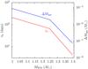 |
Fig. 1 Variation of the ignition mass of the nova ΔMign and the mass-loss timescale tml (≈decline time of the outburst by 3 mag from optical peak, t3) with the mass of the WD for the accretion rate Ṁ = 10-7M⊙ yr-1 and WD core temperature 107 K, from Yaron et al. (2005). |
To obtain the latter, we note that in the multicycle nova evolution models of Yaron et al. (2005), for fixed mass accretion rate and WD core temperature, the light-curve decay timescale is determined solely by the WD mass. Therefore, the cumulative distribution of novae over decay time is given by 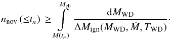 (4)Here tn is the time to decline by n mag from peak (n = 2,3), nnov( ≤ tn) is the cumulative number of novae with decline time shorter than or equal to tn and M(tn) is the WD mass corresponding to the given decline time tn (for the given values of Ṁ and TWD). As before, the inequality sign in Eq. (4)reflects the fact that the net accreted mass can be lower than the envelope ignition mass. The corresponding differential distribution is given by
 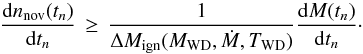 (5)As before, this distribution gives the number of novae with particular temporal properties per one type Ia supernova.
In the following, we use the results of the multicycle nova evolutionary calculations by Yaron et al. (2005). Their results for the envelope ignition mass and t3 timescale of the light curve are shown in Fig. 1. We carry out calculations for three values of the mass accretion rates – 10-7, 10-8 and 10-9M⊙ yr-1 and assume WD core temperature of 107 K. Our choice is explained below. In addition, some of the calculations in Sect. 3 are done for the mass-accretion rate of 5 × 10⁻⁷M⊙ yr-1, which is not tabulated in Yaron et al. (2005). To this end, we use the results of Hillman et al. (2015) that are based on a modified version of the code of Prialnik & Kovetz (1995). We estimate the nova ignition masses using their plot of the nova cycle duration against the mass-accretion rate (Fig. 2 in Hillman et al. 2015). As a proxy for the nova decline time t3, we use the flash duration plotted in their Fig. 7. We verified that the so-obtained nova ignition masses and t3 timescales are consistent (albeit not identical) with the interpolation of Yaron et al. (2005) results.
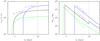 |
Fig. 2 Cumulative (left) and differential (right) t2 distributions of novae produced by one successful SN Ia progenitor, assuming that it accreted in the unstable nuclear burning regime throughout its entire accretion history. The numbers near the curves indicate the mass-accretion rate. The discontinuities in the differential distributions are caused by the discontinuity in the slope of log-linear interpolation of t2 and MWD values from Yaron et al. (2005) tabulation. They do not affect the cumulative distribution in any significant way, as can be seen in the left panel. The sharp drop in the distributions at low t2 values corresponds to the fastest novae produced by the WD near the Chandrasekhar mass limit. |
The mass loss during the nova explosion becomes more significant at lower mass-accretion rates (e.g., Yaron et al. 2005; Hillman et al. 2015). Therefore, in the context of the problem of SN Ia progenitors, only relatively high mass-accretion rates (~10-7M⊙ yr-1) are relevant. We therefore assumed the mass-accretion rate of 10-7M⊙ yr-1 in our baseline configuration, but also considered lower values of 10-8 and 10-9M⊙ yr-1 to investigate the trends with Ṁ. Some of the calculations in Sect. 3 are done for Ṁ = 5 × 10⁻⁷M⊙ yr-1 to allow direct comparison of predictions of the Hillman et al. (2015) model with observations.
Our choice of the WD core temperature is motivated by the results of Townsley & Bildsten (2004), who studied the effect of accretion on the thermal state of the WD and found an equilibrium WD core temperature of ~8−10 × 106 K for accretion rates in the range 10-9−10-8M⊙ yr-1, the temperature increasing with Ṁ. Their calculations only covered the mass-accretion rates typical for classical novae and did not extend beyond 10-8M⊙ yr-1. However, at high mass-accretion rates, ≳ 10-7M⊙ yr-1, the properties of nova outbursts do not strongly depend on the core temperature because the overlying hot He layer from previous outbursts acts as a heat barrier (Townsley & Bildsten 2004; Wolf et al. 2013). We therefore assumed a core temperature of 107 K in our baseline configuration. We investigate the dependence of our results on the core temperature in more detail in Sect. 3.
Yaron et al. (2005) provided two timescales characterizing the light-curve decay rate – the duration of the mass-loss phase tml and the decline time of the bolometric luminosity by 3 mag from maximum t3,bol. From an observational point of view, however, the timescale of interest is the decline time of the optical light from the nova. From the comparison of the results from Yaron et al. (2005) with observations, it is known that tml and t3,bol bracket t3 (Prialnik & Kovetz 1995; Yaron et al. 2005; Kasliwal et al. 2011). The shorter of these two, tml, is much closer to the observed t3 than t3,bol. We therefore proceed with tml as an approximation to t3. We investigate how our results change if we use the longer t3,bol in Sect. 3. For extragalactic novae, where the survey sensitivity2 becomes a problem, it is easier in practice to measure t2 (the time to decline by 2 mag from peak) than t3. For fast novae, the two quantities are approximately related by t2 ≈ t3/ 2.1, for the slow novae by t2 ≈ t3/ 1.75, with the transition at t3 = 50 days following Duerbeck (in Bode & Evans 2008). We mostly use t2 throughout the remainder of the paper.
For each value of the mass-accretion rate we log-linearly interpolated the ignition mass ΔMign, tml and t3,bol between the grid values of the WD mass (0.4, 0.65, 1.0, 1.25, and 1.4 M⊙) in Yaron et al. (2005). The lower integration limit in Eq. (4)was conservatively assumed to be equal to 1.0 M⊙. For Ṁ = 10-7M⊙ yr-1; this corresponds to slow novae with t3 ≈ 200 days. As the differential distribution of novae over t2 is sufficiently steep,  (see discussion of Fig. 2 below), the choice of the initial WD mass is not very important when considering the integrated nova rates, as long as it is not too close to the Chandrasekhar mass.
The so-computed cumulative and differential t2 distributions of novae are shown in Fig. 2. As expected, a significant fraction of novae produced by a successful SD SN Ia progenitor have short t2 times. For example, in our baseline calculation (Ṁ = 10-7M⊙ yr-1) we obtain the total predicted number of novae per one SN Ia ~6.5 × 10⁵. Of these, more than 60% have t2 ≲ 5 days and about 80% have t2 shorter than 10 days. The predicted number of novae grows with the mass-accretion rate, reaching ~7.7 × 10⁵ for Ṁ = 5 × 10⁻⁷M⊙ yr-1.
3. Statistics of novae in M 31
M 31 has been a hot spot for the observation of novae since the work of Hubble (1929). We have chosen this galaxy for our analysis because of its many detections. We start this section by reviewing recent supernova and nova rate measurements in M 31 and then proceed with constraining the contribution of the nova channel to the observed SN Ia rate using the results of the previous section.
3.1. SN Ia rate in M 31
The morphological type of M 31 is Sb (de Vaucouleurs et al. 1991), for which Mannucci et al. (2005) reported the stellar mass specific SN Ia rate of 6.5 × 10⁻⁴ SNe yr-1 per 1010M⊙. However, Hubble morphological classes are rather broad – indeed, for the adjacent morphological type Sbc/d, the quoted SN Ia rate is higher by a factor of ~ 2.5. Therefore, there must inevitably be some spread in the SN Ia rates between galaxies of the same morphological type. Mannucci et al. (2005) used the morphological type of the galaxy as a proxy for its star formation rate (SFR). To the first approximation, the mass-specific SN Ia rate is determined by the current SFR (e.g., Sullivan et al. 2006; see also Maoz et al. 2014) in the absence of detailed knowledge of the star formation history of the galaxy. A more accurate and continuous characterization of the current SFR of the galaxy is its color, albeit also with considerable spread. In particular, Mannucci et al. (2005) used the B−K color to quantify the dependence of the supernova rate on SFR. The extinction-corrected B−K color of M 31 within ~ 10–20 kpc from the galactic center is B−K ≈ 3.5 mag (Battaner et al. 1986). From Fig. 5 in Mannucci et al. (2005) we find the mass-specific SN Ia rate of ~ 1.0 × 10⁻³ SNe yr-1 per 1010M⊙, which is somewhat higher than inferred from its morphological type. This number is compatible with the more recent result of Li et al. (2011), who obtained a mass-specific SN Ia rate of  SNe yr-1 per 1010M⊙ in their B−K = 3.4−3.7 mag bin for a galaxy of stellar mass 1.1 × 10¹¹M⊙ (see below). Of course, the current SFR value can also be used directly. The SFR estimates for M 31 are in the range ≈ 0.4–0.8 M⊙ yr-1 (Barmby et al. 2006; Devereux et al. 1994), and with the Sullivan et al. (2006) calibration, we obtain an SN Ia rate of (0.5–0.6) × 10-3 SNe yr-1 per 1010M⊙, also compatible with the above numbers.
From the physical point of view, the SN Ia rate of the galaxy is determined by the convolution of its star formation history with the delay time distribution (DTD) of SNe Ia (Maoz & Mannucci 2012). As the former is poorly known, we used the DTD value at the delay time equal to the mean stellar age of M 31 to estimate its SN Ia rate. Olsen et al. (2006) found both the bulge and inner disk of M 31 to be dominated by old (6−10 Gyr) stellar population, and Brown et al. (2006) found the outer disk to be dominated by 4−8 Gyr old stars. Then, taking the mean age for the M 31 stellar population to be 8 Gyr and using the delay time distribution of Totani et al. (2008) we obtain a mass-specific rate of ≈ 0.7 × 10⁻³ SNe yr-1 per 1010M⊙.
Thus, different estimations give approximately consistent values of the specific SN Ia rate in M 31 in the range of ≈ (0.5–1.0) × 10-3 SNe yr-1 per 1010M⊙. In the following, we conservatively use the rate based on the result reported by Mannucci et al. (2005) for Sb galaxies, that is, 0.65 × 10⁻³ SNe yr-1 per 1010M⊙, which is one of the lower rate estimates from above. As the nova rates are directly proportional to the SN Ia rate (e.g., Eq. (3)), any higher SN Ia rate will only strengthen our conclusions. With the stellar mass of M 31 of 1.1 × 10¹¹M⊙ (Barmby et al. 2007) we obtain its SN Ia rate, ṄSNIa = 7.15 × 10⁻³ yr-1, which we use in our calculations below.
3.2. Nova rate in M 31
Altogether, there are more than 9003 novae detected in the direction of M 31 (e.g., Hubble 1929; Arp 1956; see also Capaccioli et al. 1989). However, the majority of the existing nova catalogs lack an accurate incompleteness analysis, which renders them unsuitable for use in our calculations.
Completeness of a nova survey is determined by the usual factors, such as spatial variation of the sensitivity caused by incomplete coverage of the survey, variation of the surface brightness of the galaxy, and extinction. In addition, it is determined by the factors related to the transient nature of the sought objects, such as temporal sampling of the survey and variation in the light-curve morphology. The most thorough completeness analysis to date among the nova surveys was performed for the nova catalog produced in the course of the recent POINT-AGAPE (Pixel-lensing Observations with the Isaac Newton Telescope − Andromeda Galaxy Amplified Pixels Experiment) survey (Darnley et al. 2004). The POINT-AGAPE nova catalog was produced by an automated detection pipeline, thus permitting an objective characterization of its completeness (many even relatively recent nova surveys relied on some form of a visual inspection of the images and/or light curves, which makes their completeness difficult to compute accurately). Darnley et al. (2006) carried out a careful analysis of the completeness of the detection pipeline and the survey itself. To this end, they seeded the raw POINT-AGAPE data with resampled light curves of their detected novae. This allowed them to compute the completeness of the POINT-AGAPE nova catalog and to obtain a robust estimate of the underlying global nova rate in M 31. As a result of these analyses, they produced the global nova rate of  yr-1.
yr-1.
3.3. Contribution of novae to the SN Ia rate
With the nova rate known, we estimated the maximal SN Ia rate these novae can produce as follows 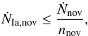 (6)where ṄIa,nov is the SN Ia rate that may be produced by novae, nnov is the number of novae produced by one successful SN Ia progenitor (cf. Eq. (3)), and Ṅnov is the observed nova rate. We note that Eq. (6)gives an upper limit on the nova contribution to the SN Ia rate for at least two reasons: (i) Eq. (3)gives only the lower limit of the number of novae per SN Ia, as discussed in Sect. 2; (ii) obviously, not all novae reach the Chandrasekhar mass limit.
However, before the nova rate of 65 yr-1 can be inserted into Eq. (6), the following should be considered. The POINT-AGAPE nova catalog does not contain very fast novae with t2 ≲ 10 days in the r′-band. Therefore, as discussed in Darnley et al. (2006), their completeness modeling is only sensitive to novae with an r′-band t2 between 9.80 days (the fastest nova in their catalog) and 213.12 days (the slowest nova). In this t2 range, there was no strong evidence suggesting large variation in the completeness as a function of t2, the only variation being, as expected, spatial (Matt J. Darnley, priv. comm.). Therefore, for a fair comparison, nnov in Eq. (6)should be the number of novae with light-curve decay times in the range 10 ≲ t2 ≲ 213 days. Because of the steepness of the differential distribution dnnov/ dt2 (Fig. 2), the latter is nearly equivalent to t2 ≥ 10 days4.
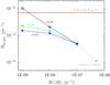 |
Fig. 3 Maximal contribution of novae to the SN Ia rate of M 31 as a function of assumed mass accretion rate for different values of WD core temperature as indicated by the numbers near the curves. The point at Ṁ = 5 × 10⁻⁷M⊙ yr-1 (shown in gray) is computed from the models of Hillman et al. (2015); other points are computed based on Yaron et al. (2005) nova models. The red solid line shows the M 31 supernova rate. |
The maximal supernova rate computed from Eq. (6)is shown in Fig. 3. As can be seen, our baseline model (Ṁ = 10-7M⊙ yr-1) predicts the maximal SN Ia rate of ≈ 5.0 × 10⁻⁴ yr-1. For the mass-accretion rate of Ṁ = 5 × 10⁻⁷M⊙ yr-1 considered by Hillman et al. (2015), the maximal SN Ia rate becomes ≈ 1.1 × 10⁻⁴ yr-1. Interestingly, for lower mass-accretion rates, observed population of novae could in principle explain a larger fraction of SNe Ia, and for very low rates, Ṁ ≲ 10-9M⊙ yr-1, and low WD temperature, the predicted rate is compatible with the observed value. However, such low mass-accretion rates are believed to be irrelevant as regards the nature of SN Ia progenitors (Sect. 2). For the mass-accretion rates in the range ~ (1−5) × 10-7M⊙ yr-1, which are typically considered in this context, the maximal contribution of novae to the observed SN Ia rate is limited to ≈ 2−7%.
The upper limit on the contribution of novae to the SN Ia rate decreases by a few times if we use t3,bol instead of tml in the models of Yaron et al. In this case, the supernova rate predicted in our baseline model is ≈ 1.8 × 10⁻⁴ yr-1, which is ~ 40 times lower than the observed SN Ia rate. At lower mass-accretion rates and WD temperatures, the maximal supernova rate is ~5−10 times short of the observed value.
In the above calculation, we ignored the possible difference of the observed novae in the WD composition. In particular, some fraction of the observed nova outbursts may be hosted by oxygen-neon (ONe) WDs (Truran & Livio 1986; Ritter et al. 1991; Gil-Pons et al. 2003; Shore et al. 2013). For example, for the Galactic novae, Gil-Pons et al. (2003) estimated this fraction to be about ~ 1/3 of nova outbursts. The ONe WDs are known to undergo accretion-induced collapse upon reaching the Chandrasekhar mass limit, rather than producing SNe Ia, and therefore they should be excluded from our calculation of the contribution of novae to the supernova rate. This is not possible because the composition of the WD host in the majority of observed novae is unknown. However, Eq. (6)gives an upper limit for the nova contribution to the supernova rate and inclusion of some number of ONe novae in the nova rate does not invalidate it. Although the upper limit may be tightened somewhat by using the (unknown) pure CO nova rate, the results of Gil-Pons et al. (2003) suggest that the improvement will not be dramatic. Moreover, the POINT-AGAPE sample is dominated by the relatively slow novae with t2 ≳ 10 days, which, according to the models of Yaron et al., are hosted by relatively lower mass WDs (cf. Fig. 1). Therefore the POINT-AGAPE sample is probably less contaminated by ONe novae (which are typically hosted by more massive WDs) than the overall population of novae.
3.4. Fast novae
About ~ 80% of the novae produced by a typical successful (unstably burning) SD SN Ia progenitor have short decay times, t2 ≲ 10 days (Sect. 2, Fig. 2). If a fraction f of the total number of SN Ia progenitors in M 31 accrete in the unstable nuclear burning regime while accumulating their final ΔM ≈ 0.1 M⊙ (i.e., from M ≈ 1.3 M⊙ to Mch), fast novae with t2 ≲ 10 days5 should be produced at a rate of ≳ 3.6 × 10³ × f, assuming Ṁ = 10-7M⊙/yr. For example, if all the novae from the POINT-AGAPE sample were to reach the Chandrasekhar mass limit, the fast novae would be produced at a rate of ~ 200−300 yr-1.
Such fast novae have not been detected in the POINT-AGAPE survey, either because they are rare in M 31 or because the survey was not sensitive to them, or a combination of these two reasons (Darnley et al. 2006). From results of other surveys, we know that some number of such fast novae do exist, an example being the famous M 31N 2008-12a (Shafter et al. 2012; Darnley et al. 2014; Henze et al. 2014; Tang et al. 2014; see also the MPE optical nova catalog from footnote 3), but their true frequencies in the bulge and the disk of the galaxy remain to be determined.
From the above it is obvious that statistics of fast novae could provide a powerful tool for investigating the populations of massive WDs with unstable nuclear burning and for further constraining their contribution to the observed SN Ia rates. Accurate determination of their frequency is, however, hindered because they are difficult to detect as a result of their short lifetimes; this demands surveys with a very high cadence. For example, the famous M 31 nova, M 31N 2008-12a, was only discovered to be a recurrent nova in 2008, although it explodes every year. This is discussed in the following section, where we investigate how completeness of a nova survey depends on its temporal sampling.
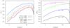 |
Fig. 4 Detection efficiency for novae in M 31 as a function of their decline time t2 for surveys with the limiting magnitude of mR = 20 and different temporal sampling (left) and for surveys of different limiting magnitudes with observations performed every night (right). The decline of the detection efficiency for slow novae is caused by their lower peak magnitudes and the finite time span of the simulated survey (see Sect. 4). |
4. Temporal sampling and completeness of nova surveys
In this section we investigate how efficiently fast novae can be detected in surveys of various sensitivity and cadence. Our goal is to identify typical requirements with respect to the temporal sampling and limiting magnitude of a modern CCD survey aimed to characterize the population of fast novae, rather than to substitute the actual completeness calculations. The latter should be performed taking into account the characteristics of the particular survey and parameters of its detection pipeline. We therefore do not include in our calculations the full complexity of the light-curve shapes, replacing it with a simple template (albeit derived from observed nova light curves), with its peak magnitude drawn from the range sampled by observed novae. We do, however, take into account spatially varying internal extinction in M 31 and contribution of its unresolved surface brightness to the statistical noise in the image, that is, to the sensitivity in detecting novae. We conduct our simulations for a PTF-class telescope (1.2 m Samuel Oschin Telescope at the Palomar Observatory).
We employed the following procedure. First, based on observed novae, we produced a scalable light-curve template (Appendix A), which we used to model the light curve of a nova with a given peak magnitude and t2 time. To draw the peak magnitude of the nova with the given t2, we produced an analog of the classic MMRD relation from a large, heterogenous set of observational data, with the main goal to sample the range of observed magnitudes as fully as possible (Appendix B). We then performed Monte Carlo simulations of the nova detection process. In these simulations, we randomly seeded a large number of novae distributed across the face of the galaxy for each value of t2 and determined how often they are detected in a survey of a given limiting magnitude and temporal sampling6. The simulations were carried out in R-band because this is the band used in many recent nova surveys of M 31.
To determine the nova detection sensitivity, we considered the following. The noise in an image pixel containing S = SM 31 + Ssky counts (in DN unit) accumulated during the exposure time texp can be expressed as 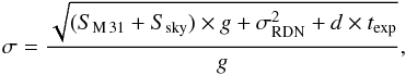 (7)where g is the gain, σRDN the readout noise, and d the dark current (see Howell 2006). For these, we assumed typical parameters of the PTF survey (Law et al. 2009) – 1.6 e-/DN, 12 e- and 0.1 e-/s, respectively. For the Ssky we assumed typical Palomar sky brightness for photometric gray nights (Law et al. 2009; Laher et al. 2014). For the SM 31, we used the SDSS mosaic image of M 31 from Tempel et al. (2011), which we converted from Sloan-r to R-band using the relation from Blanton & Roweis (2007). We ran this image through SEXTRACTOR (Bertin & Arnouts 1996) to generate the unresolved surface brightness map of the galaxy. Since the SDSS mosaic image is sampled at a larger pixel scale (3.96′′) than that of the PTF (1.01′′), we reduced the pixel counts S from the SDSS image by ≈ 15.4. The radius of the aperture used for measurement of a star is typically on the order of its FWHM (e.g., Mighell 1999), which is ≈ 2′′ for PTF images (Law et al. 2009). We therefore multiplied the pixel σ from Eq. (7)by a factor of ≈ 4 to obtain the effective rms noise for point source detection: σps = 4σ. In our simulations, we conservatively assumed a 10σps threshold for detecting novae.
We parameterized our simulations by the nominal limiting magnitude (mlim) of the survey, which is related to the exposure time by the following for the sky-limited case that is typical of modern surveys  (8)Here ZP is the zero point of the photometric calibration and σsky is the noise from the sky background in a typical aperture for star flux measurement. The latter is obtained from Eq. (7)with S = Ssky and appropriate aperture correction as described above.
The intrinsic extinction map of M 31 was computed based on the results of Tempel et al. (2011) to which a constant foreground reddening of AR = 0.15 (Shafter et al. 2009) was added. The extinction was applied to all the seeded novae, depending on their spatial location in M 31. However, its overall impact on the detection completeness does not exceed a few percent.
Taking into account the visibility of M 31 from the northern hemisphere (between August and March), we assumed the survey duration to be 211 days. For every decline time t2 in the range of interest, we seeded at every pixel of the SDDS image 20 000 novae occurring randomly in time within the survey time span. To each of the simulated novae, we assigned a peak magnitude that was drawn randomly from a Gaussian distribution with the mean and standard deviation as computed in Appendix B (Fig. B.1, Table B.1). The nova light curve was generated using the template derived in Appendix A, rescaled to have the desired t2 and peak magnitude, Eq. (A.1)and then the extinction was applied. The detection efficiency was determined for every pixel of the SDSS image as the ratio of the number of detected novae, whose decline time t2 could be measured, to the total number of seeded novae. To obtain the overall efficiency η(t2), these values were then averaged across the image, with the weights proportional to the stellar mass contained in the given pixel (i.e., we assumed that the nova rate scales with the stellar mass). To characterize the latter, we used the Spitzer 3.6 micron mosaic image of M 31 by Barmby et al. (2006). We thus computed the completeness curves for every survey configuration we had set up, determined by the observing pattern (every night, second night, third night, 75% and 50% random coverage) and limiting magnitude (19 to 22 mag).
The results of these simulations are plotted in Fig. 4. As expected, the detection efficiency declines toward short t2 because novae with shorter t2 times fade away faster and therefore are less likely to be detected than their longer lasting counterparts. On the other hand, the detection efficiency also drops toward long t2. This is caused by the combined effect of their lower peak magnitudes (Fig. B.1) and the finite observation time span. The latter is obviously determined by the survey duration. For example, a survey conducted in two consecutive years would have a better detection efficiency for slow novae than those shown in Fig. 4 (but the same for short novae).
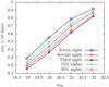 |
Fig. 5 Fraction of all fast novae with t2 ≤ 10 days detected in surveys of different temporal sampling as a function of their limiting magnitude. It is assumed that the distribution of novae over decay times dnnov(t2)/dt2 is given by Eq. (5)for a mass accretion rate of Ṁ = 10-7M⊙ yr-1. |
The cumulative efficiency of the survey (i.e., the fraction of all novae with the t2 time shorter than a given value that are detected in the survey) depends on dnnov/ dt2 – the expected distribution of novae over t2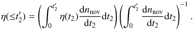 (9)The true distribution dnnov/dt2 is unknown, however. For example, in the “vanilla” SD scenario from Sect. 2, the distribution is given by Eq. (5). The result for Ṁ = 10-7M⊙ yr-1 is shown in Fig. 5 for surveys of different temporal sampling as a function of their limiting magnitude. This plot shows that a high-cadence survey with a limiting magnitude of mR = 22 will detect about ≈80–90% of fast novae (t2 ≤ 10 days). To detect more than 50% of fast novae in a survey with observations conducted every night, its limiting magnitude has to be better than mR ≈ 20. If observations are carried out every third night, a limiting magnitude of mR ≈ 20.5 is required.
To see how the detection efficiency translates into absolute numbers of novae, we consider the recent PTF survey of M 31 as an example. PTF has been conducting regular and frequent M 31 observations during the corresponding visibility periods (approximately from July/August to December/January). From Fig. 2 of Cao et al. (2012) we estimate that the observing schedule typically covers ≈ 50–80% of the nights during these periods every year. For the 5-sigma limiting magnitude of mR ≈ 20.6 (Law et al. 2009), we estimate from Fig. 5 the detection efficiency of ~55−65%. The “vanilla” SD scenario predicts about ≈ 3600 fast (t2 ≤ 10 days) novae per year in M 31. One should also take into account that the M 31 visibility periods for the PTF telescope cover approximately 0.5 yr. We therefore predict that the PTF survey of M 31 should be detecting of the order of ~1000 × f fast (t2 ≤ 10 days) novae per observing season7, where, as before, f is the fraction of SNe Ia accreting in the unstable nuclear burning regime shortly before the explosion (at MWD > 1.3 M⊙). Furthermore, if all the observed POINT-AGAPE novae were to become SNe Ia (i.e., f = 0.07), a PTF program with regular monitoring of M 31 several times per week should be detecting ~70 fast novae per observing season7. These numbers are significantly larger than the currently observed rate of fast novae, suggesting that f ≪ 1.
5. Discussion
With the progenitors of SNe Ia still eluding direct detection, there is a growing consensus that they may be a heterogenous class of objects united by the final outcome – thermonuclear disruption of the WD. Among other possibilities, various types of accreting binary systems have been proposed as a candidate. The fate of the accreted material is mainly determined by the WD mass and the mass accretion rate (e.g., Fujimoto 1982; Nomoto et al. 2007; Wolf et al. 2013). In the picture that has become fairly standard, there is a rather narrow range of the mass-accretion rates around ~ afew × 10-7M⊙ yr-1 (varying with the WD mass) in which the nuclear burning is steady and proceeds at the rate determined by the supply of the material through the accretion process. Below this range, the nuclear burning is subject to thermal instability, giving rise to the phenomenon of novae. In the classical picture, copious amounts of material are lost in the nova explosion, especially at the lower mass-accretion rates (Ṁ ≲ 10-7−10-8M⊙ yr-1 in the Yaron et al. 2005 calculations, for example), rendering the growth of the WD mass impossible or insignificant in the context of SN Ia progenitors. Importantly, several authors have found that the transition from unstable to stable burning is sharp – there is a discontinuity in the stability of burning, with the large amplitude flashes occurring very close to the stability strip (e.g., Wolf et al. 2013; Kato et al. 2014).
However, the main aspects of this picture have been contested by several authors. First, the existence of the stability strip has been questioned (e.g., Idan et al. 2013; Starrfield 2014; Hillman et al. 2015). In fact, no stable burning is reported in the Yaron et al. (2005) tables either, although the ejected mass becomes zero at the highest mass-accretion rates. Second, it has been suggested that mass accumulation at appreciable rates is possible in the broad range of the mass-accretion rates, including those traditionally considered to be associated with the nova regime. In fact, it has been claimed that any mass accumulation by the WD is associated with regular thermonuclear explosions (e.g., Starrfield 2014; Hillman et al. 2015). In a related development, progenitor models have been proposed that involve WDs accreting in the presumably unstable nuclear burning regime throughout or at least a part of their accretion history (e.g., Starrfield et al. 1985; Hachisu & Kato 2001; Hillman et al. 2015). Further support for these ideas is lent by the realization that recurrent novae (RNe) may host WDs with masses very close to the Chandrasekhar mass limit, the most famous example being RS Oph (Sokoloski et al. 2006; Hachisu & Kato 2001). This led to the suggestion that novae in general and recurrent novae in particular may be an important channel producing some (unknown) fraction of SNe Ia (see, for example, Wood-Vasey & Sokoloski 2006; Patat et al. 2011; Hachisu & Kato 2001; Pagnotta & Schaefer 2014).
In this paper, we pointed out that the population of WDs with unstable nuclear burning, sufficient to account for a non-negligible fraction of SNe Ia, would reveal themselves through significantly enhanced nova rates in galaxies. We thus propose that the contribution of novae to the observed SN Ia rates can be assessed through the nova statistics in nearby galaxies. We demonstrated that given the completeness-corrected nova rate in M 31 of ≈ 65 yr-1 (Darnley et al. 2006), novae can only produce a small fraction of SNe Ia, at the maximal rate of ≲ (1−5) × 10-4 yr-1, assuming typical mass-accretion rates of progenitors in the range, Ṁ ~ (1−5) × 10-7M⊙ yr-1. This constitutes no more than 2–7% of the total SN Ia rate in M 31. Moreover, we predicted that M 31 surveys of the PTF class should be detecting on the order of 1000 × f fast (t2 ≤ 10 days) novae every year, where f is the fraction of SNe Ia accreting in the unstable nuclear burning regime shortly before the explosion (at M > 1.3 M⊙). The fact that < 50 such fast novae have been recorded/detected in the course of about a century of M 31 monitoring (see the optical nova catalog maintained by MPE from footnote 3) suggests that the fraction f is small, on the order of f ≲ 10-3. However, an accurate completeness analysis of the M 31 PTF survey is needed before a robust quantitative conclusion can be made.
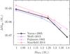 |
Fig. 6 Comparison of the ignition mass of the nova as computed by different authors. The ignition mass is shown as a function of the WD mass for a mass accretion rate Ṁ = 10-7M⊙ yr-1. The Wolf et al. (2013) results are obtained from their Fig. 8; Fujimoto (1982) from their Fig. 7; Starrfield (2014) from their Figs. 2, 3. |
Equation (3)shows that the calculation of the total number of novae per SN Ia depends on the theory of thermonuclear burning on the WD surface only through the ignition mass ΔMign. This quantity is derived from sufficiently well understood physical principles and has been computed by a number of groups (for example, Fujimoto 1982; Townsley & Bildsten 2004; Yaron et al. 2005; Wolf et al. 2013; Kato et al. 2014 and others). A comparison of some of the results is shown in Fig. 6. The plot shows that results of different calculations agree quite well, within a factor of ~2. The agreement is quite good even between authors drawing opposite conclusions regarding the existence of the stability strip. In the parameter range of interest, there is a good agreement between analytical (Fujimoto 1982) and more sophisticated numerical calculations, as well as between single flash (Fujimoto 1982; Starrfield 2014) and multicycle (Yaron et al. 2005; Wolf et al. 2013) calculations. We note that the latter two probably provide a more accurate representation of the accreting WD, and their results agree to much better than a factor of ~2. We thus conclude that the calculations of the total number of novae produced by an SD SN Ia progenitor presented in this paper are sufficiently robust and do not depend on the details of the underlying nova models, including their conclusions regarding the existence of the stability strip.
In our calculations we used the results of Prialnik & Kovetz (1995) and Yaron et al. (2005), who computed the most extensive grid of multicycle nova evolutionary models to date. The ignition masses from their calculations agree well with the results of other groups, as already discussed above (Fig. 6). Furthermore, the grid of their models covers the parameter space occupied by the observed novae well and approximately reproduces observed correlations between various nova parameters (Prialnik & Kovetz 1995; see also Walder et al. 2008). The peak magnitudes and light-curve decay times predicted by their models are compared with observations in Fig. 7. Each curve in this plot corresponds to a given combination of Ṁ and TWD, with MWD changing along the curve. Ṁ extends from 10-7 to 10-11M⊙ yr-1, thus covering the typical range expected in nova host systems. Peak magnitudes in the visual band were computed from the peak bolometric luminosity reported in Prialnik & Kovetz (1995) and Yaron et al. (2005) by applying the bolometric correction of an A5V star, as is commonly done in such estimates (Shafter et al. 2009; Kasliwal et al. 2011). The light-curve decay times were computed from the mass-loss times as explained in Sect. 2.
Figure 7 shows that the observed range of the light-curve decay times t2 is fully sampled by the nova models with WD masses varying from ≈0.4−0.65M⊙ to ≈1.3−1.4M⊙. The models also reproduce the average trend in the peak magnitude with t2 quite well. The small offset in magnitude between the models and data is reduced further if one takes into account that the theoretical models may underestimate the true value by up to 0.75 mag, as discussed in Prialnik & Kovetz (1995). These models, however, do not reproduce the scatter seen in the observed data. This suggests that the scatter may be caused by additional factors, other than those already included in the calculations of (Yaron et al. 2005; e.g., orientation effects and interaction of the ejecta with the disk and the donor star). For this reason, we used the parameters of observed novae to draw the nova peak magnitudes in our Monte Carlo simulations in Sect. 4. However, the overall agreement between the models of Yaron et al. (2005) and the data suggests that the models reproduce the global characteristics of the nova light curves sufficiently well.
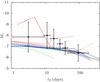 |
Fig. 7 Comparison of the data shown in Fig. B.1 with the results of multicycle nova models of Yaron et al. (2005). The black triangles and vertical error bars show the average peak magnitudes and their rms deviation for the novae grouped in equipopulated bins over the t2 time, and the curves are corresponding relations for the nova models of Yaron et al. (2005). The red, green and blue curves correspond to WD core temperature of 107 K, 3 × 10⁷ K and 5 × 10⁷ K, respectively. The solid curves are for Ṁ = 10-7M⊙ yr-1, dashed curves for Ṁ = 10-8M⊙ yr-1, short dashed curves for Ṁ = 10-9M⊙ yr-1, dotted curves for Ṁ = 10-10M⊙ yr-1, and dot-dashed curves for Ṁ = 10-11M⊙ yr-1. |
The famous recurrent nova M 31N 2008-12a appears to be somewhat (by about ~ 1–2 mag) underluminous as compared to the predictions of Yaron et al. (2005) as well as to its counterparts with similarly short decay times (Fig. B.1). Of course, it may be just a faint tail of the distribution approximately centered near the value predicted by Yaron et al. (2005) for the corresponding range of decay times. However, there is another possibility: it might present the bright tail of the so far unknown population of fast and underluminous novae hosted by massive WDs near the Chandrasekhar mass limit. Although intriguing, this possibility seems at present less likely. The main argument is that M 31N 2008-12a is up to three magnitudes brighter than the typical sensitivity limit of the PTF M 31 survey, and despite about six years of continuous PTF observations (since August 2009), no other similar nova was discovered. A more quantitative analysis of the latter possibility is beyond the scope of this paper.
Shafter et al. (2015) have undertaken a census of the recurrent nova population in M 31 based on the positional coincidence of about ~103 novae recorded in modern astronomy. They identified 16 recurrent novae and candidates, but they estimated that the detection efficiency of the recurrent systems may be as low as ~10% of that of classical novae. Based on these data and assuming that recurrent nova systems typically accrete at 10-7M⊙ yr-1, they constrained their contribution to the SN Ia rate at the level of ≲ 2%. This upper limit is comparable to the limits we derived here. In particular, for the 10-7M⊙ yr-1 accretion rate, we constrained the contribution of all slow (t2 ≳ 10 days) novae, irrespective of their recurrence times, to ≲ 7%.
The upper limit of ≈ 2–7% we obtained is comparable to the upper limits on other versions of the SD scenario. Based on the luminosity of unresolved soft X-ray emission in a sample of nearby elliptical galaxies observed by Chandra, Gilfanov & Bogdán (2010) constrained the contribution of supersoft X-ray sources (i.e., stably nuclear burning WDs located in the stability strip) to ≲ 5%. Johansson et al. (2014) used the recombination line λ4686 Å of HeII to limit the EUV emission from lower temperature sources – those that escaped the X-ray based analysis of Gilfanov & Bogdán (2010) due to their very soft spectra and absorption by the ISM. Such low-temperature sources can be associated with the low-mass WDs or with the rapidly accreting sources above the stability strip (Hachisu et al. 1996). In particular, Johansson et al. (2014) applied the diagnostics suggested by Woods & Gilfanov (2013) to stacked SDSS spectra of ~104 retired galaxies and constrained the contribution of accreting WDs with photospheric temperature in the range ~ (1.5–6) × 105 K to ≲ 5–10%. These upper limits can be tightened further and their photospheric temperature range can be extended using intrinsically brighter forbidden lines of metals (Woods & Gilfanov 2014). In particular, Johansson et al. (in prep.) used the λ6300 Å forbidden line of neutral oxygen to derive an upper limit of aboutafew per cent on the contribution of accreting WDs with the photospheric temperature in the ~105–106 K range. Combined together, these constraints limit the role of the main variations of the SD scenario in producing SNe Ia. Even when (very conservatively) summed independently, their total contribution to the observed SN Ia rate cannot exceed ≲ 10–20%. Alternatively, a typical supernova could not have accreted more than ≲ 0.03−0.05M⊙ in each of the above mentioned regimes – that is, below, in, or above the stability strip.
We assumed, as is commonly accepted (e.g., Maoz et al. 2014), that SNe Ia are produced by the WDs exploding at the Chandrasekhar mass. However, sub-Chandrasekhar (e.g., Woosley & Weaver 1994; Bildsten et al. 2007; Sim et al. 2010; Kromer et al. 2010) as well as super-Chandrasekhar (e.g., Howell et al. 2006; Liu et al. 2010; Kamiya et al. 2012) detonations are also being considered by a number of authors. If sub-Chandrasekhar detonations contribute significantly to the SN Ia rate, the nova-based constraints may need to be relaxed. Indeed, if a WD explodes before reaching the Chandrasekhar mass, the distribution shown in the right panel of Fig. 2 will be cut off at the t2 time, corresponding to the explosion mass (cf. Fig. 1). Correspondingly, the upper limit on the contribution of novae to SN Ia production will increase, as nnov in Eq. (6)decreases. For example, if a typical SN Ia progenitor WD explodes at 1.3 M⊙, the entire population of fast novae (t2< 10 days) will not be produced by the sub-Chandrasekhar supernova progenitors, but the constraints derived form the POINT-AGAPE survey will still hold in full. Obviously, in this scenario the observed fast novae are not the progenitors of sub-Chandrasekhar supernovae. If the typical explosion mass is even lower, for example, 1.1 M⊙, current nova statistics become unconstraining. In the super-Chandrasekhar models the result depends on the properties of nova explosions on the surface of a rotating WD, which are currently not well understood. However, at present there is no evidence that either sub- or super-Chandrasekhar models contribute dominantly to the SN Ia rates, therefore constraints on the nova-channel derived in this paper should hold for the bulk of supernovae.
Finally, we note that we used M 31 galaxy to tune our calculations and compare their results with observations because of its proximity and relatively well-known nova population. However, our results can be easily generalized to other galaxies of similar age. Observations of several nearby galaxies show that they have comparable nova rates per unit stellar mass (e.g., Shafter et al. 2014). As the same is true for the supernova rates in galaxies of similar morphological type, the constraints on the contribution of the nova channel to supernova rate are expected to apply to other nearby galaxies of similar age and morphological type.
6. Conclusions
We propose that the statistics of novae in nearby galaxies is a sensitive diagnostic of the population of accreting WDs with unstable nuclear burning and can be used to constrain the role of this channel in producing SNe Ia. Using multicycle nova models of Yaron et al. (2005), we computed the number and temporal distribution of novae produced by a successful SN Ia progenitor, assuming that it accretes in the unstable nuclear burning regime throughout its accretion history. We predicted the total number of novae to be ≈ 6.5–7.7 × 10⁵ per supernova, assuming that a typical SN Ia progenitor accretes material at the rate of ≈ (1−5) × 10-7M⊙ yr-1. Using the nova rate in M 31 as measured by the POINT-AGAPE survey, ≈ 65 yr-1 (Darnley et al. 2004, 2006), we estimated the maximal contribution of the nova channel in producing SNe Ia. Considering relatively slow novae, with light-curve decay times t2 ≳ 10 days, whose characteristics are compatible with the observed novae from the POINT-AGAPE catalog (Darnley et al. 2006), we concluded that their contribution to the observed SN Ia rates cannot exceed ≈ (1−5) × 10-4 yr-1. This constitutes less than 2–7% of the total SN Ia rate in M 31.
An even more sensitive diagnostic can be provided by fast novae, which originate from the most massive WDs and are characterized by the lowest ignition masses. To use their potential, high-cadence nova surveys are required. We investigated how the detection efficiency of a generic nova survey of M 31 depends on its limiting magnitude and temporal sampling. We found that a survey with a limiting magnitude of mR ≈ 22 will detect about ≈ 80−90% of the predicted fast novae (t2 ≲ 10 days) provided that observations are conducted at least every second or third night. To detect more than 50% of such novae in a survey with observations carried out every night, its limiting magnitude has to be mR ≳ 20. Such surveys are expected to detect on the order of ≳ 1000 × f fast novae per observing season in M 31, where f is the fraction of SN Ia progenitors that accreted in the unstable nuclear burning regime while accumulating the final ΔM ≈ 0.1 M⊙ before the supernova explosion. This is significantly larger than the currently observed rate of fast novae in M 31, suggesting that f ≪ 1. However, high-cadence surveys with accurately characterized completeness are required to place robust constraints on the value of f. Existing and upcoming surveys such as the PTF, Pan-STARRS, and LSST are well-suited for this task.
The predicted number of novae per SN Ia should not depend strongly on the details of the underlying nova models because they are only determined by the ignition mass of the envelope. This quantity is derived from sufficiently well understood physical principles, and the results of computations by different groups agree quite well, even among those at odds about the existence of the stability strip. The division of the total number between slow and fast novae depends on the assumptions made about the shape of their light curves. To this end, we used the multicycle nova models of Yaron et al. (2005), which are known to sample the observed range of the nova decay times correctly and reproduce various correlations between observed nova properties. Calculations based on two different timescales tabulated in Yaron et al. (2005) – mass-loss and bolometric, give similar results leading to the same conclusions. Finally, in our incompleteness simulations we used the observed nova light curves and their peak magnitudes, therefore these results are independent of the theoretical nova models.
Online material
Appendix A: Nova light-curve template
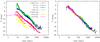 |
Fig. A.1 Light curves of the sample selected from the S class of the catalog compiled by Strope et al. (2010) with all the peaks aligned at t = 10 days by a linear shift along the time axis (left) and the resulting transformed curves after stretching in time and shifting in magnitude with respect to the reference light curve of V1668 Cyg according to Eq. (A.1)(right). |
Nova light curves are known to have a variety of shapes. In an effort to classify them, Strope et al. (2010), using a sample of 93 well-observed Galactic novae, have proposed seven morphological classes. Of these, the smooth (S) class is the most fundamental since the other light-curve shapes can be derived from the smooth class by superposing it with various features. The largest fraction of novae in the sample of Strope et al. (2010; 38%) falls in the S class; more than half of the novae with t3 ≤ 21 days (taking this value to define the fast novae of interest) belong to this class as well. Furthermore, in our simulations, we used light curves within 2−3 mag from the peak, where they generally have a smooth morphology (most of the features defining the distinction between the various classes typically develop much later in time). We thus adopted the S-class light curves to generate the template curve as described below.
We selected all sufficiently well sampled S-class light curves from Strope et al. (2010). In Fig. A.1, these light curves are shown with their peaks aligned by shifting linearly along the time axis. We then used the following transformation to match the light curves: ![\appendix \setcounter{section}{1} \begin{equation} \label{eq:transformation} m(t)\rightarrow m'(t')=\Delta{m}+m[(t-t_{p})s], \end{equation}](/articles/aa/full_html/2015/11/aa24118-14/aa24118-14-eq225.png) (A.1)where m(t) is the magnitude in the frame t, m′(t′) is that in the transformed frame t′ = (t−tp)s, tp is the time of the peak of the light curve, Δm the magnitude shift, and s the time stretch factor.
(A.1)where m(t) is the magnitude in the frame t, m′(t′) is that in the transformed frame t′ = (t−tp)s, tp is the time of the peak of the light curve, Δm the magnitude shift, and s the time stretch factor.
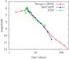 |
Fig. A.2 Co-aligned template light curves from the three nova samples, viz., the Galactic sample from Strope et al. (2010) and the M 31 samples obtained from the WeCAPP and PTF nova catalogs. |
The light curves were transformed to match the reference light curve, for which we chose V1668 Cyg. To this end, we binned the light curves logarithmically (typically five bins or more per dex along the time axis) and determined the magnitude in each bin by taking the average, weighted by the inverse square of the uncertainty in the individual magnitude measurement. The best-fit parameters Δm and s of the transformation Eq. (A.1)were determined by minimizing the χ2. The result of this procedure is shown in the right panel in Fig. A.1. In all cases we were able to obtain a reasonably good agreement, with the values of the stretch factor ranging from ≈ 0.5−2 and the rms dispersion between the reference and individual lightcurves calculated down to 6 mag from the peak being in the range 0.18–0.33 mag. Finally, we averaged the resulting transformed curves by binning in time (logarithmically again) and weighting by the respective uncertainties to produce the template curve.
This template light curve was generated using a Galactic nova sample. Although we do not expect any significant difference from the M 31 novae, for a consistency check we compared our template with light curves from two different M 31 nova samples. We applied the procedure described above to the selection of well-sampled light curves from the nova catalog of the WeCAPP (Riffeser et al. 2001), which have been classified as having smooth morphology (Lee et al. 2012), and to light curves from the PTF M 31 survey in Cao et al. (2012). In these two cases, we were also able to obtain good light curve matches, with the rms dispersion (calculated down to 4 mag from peak) lower than ≈ 0.30 mag. Final template curves were generated using the same procedure as before. The resulting templates are shown in Fig. A.2 along with our default template based on Strope et al. (2010) data. The plot shows that all three templates agree very well with each other. For our calculations, we used the template obtained based on the Strope et al. (2010) data because it is the best sampled and covers the broadest magnitude range.
Appendix B: Peak magnitudes of novae
For each simulated nova we need to assign some value for its peak magnitude. To this end, we produced an analog of the MMRD relation with the caveats detailed below. Various forms of this relation have been obtained previously (for example, see della Valle & Livio 1995; Downes & Duerbeck 2000; Darnley et al. 2006; Shafter et al. 2011), although recently its existence has been questioned (Kasliwal et al. 2011). However, for the purpose of this study, we are not concerned with the existence of the MMRD relation, instead we need to account for the full range of observed nova peak magnitudes in our simulations. We therefore collected a large sample of novae and determined their mean magnitudes and rms scatter in broad bins over t2 as explained below.
We used the light curves from the PTF (Cao et al. 2012) and WeCAPP (Lee et al. 2012) nova catalogs with morphological classification available, the light curves from Shafter et al. (2011) that have been observed in the V-band, the high-quality light curves from Capaccioli et al. (1989), and the sample of extragalactic novae discovered by P60-FasTING (Kasliwal et al. 2011). To this compilation, we added the recently discovered very fast recurrent nova M 31N 2008-12a in M 31 with the shortest known recurrence period of ~ 1 yr (Shafter et al. 2012; Darnley et al. 2014; Henze et al. 2014; Tang et al. 2014). The PTF and WeCAPP light curves were converted from R-band to V-band using the color (V−R)° = 0.16 (Shafter et al. 2009) after accounting for the foreground extinction of AR = 0.15 (Shafter et al. 2009) estimated using a reddening of E(B−V) = 0.062 along the line of sight to M 31 from Schlegel et al. (1998). The light curves from Capaccioli et al. (1989) were corrected for foreground extinction using Apg = 0.25 (Shafter et al. 2009) and converted from the photographic band to V-band using the colors (B−mpg)° = 0.17 (Capaccioli et al. 1989; Arp 1956) and (B−V)° = 0.15 (Shafter et al. 2009). The Kasliwal et al. (2011) light curves were converted from g-band to V-band using the transformation relation from Jordi et al. (2006). Apparent magnitudes were converted to absolute magnitudes using a distance modulus of 24.36 for M 31 (Vilardell et al. 2010). Light curves from Shafter et al. (2011) were corrected for extinction and converted to absolute magnitude in the original publication. Except for the WeCAPP sample, we used the light-curve decline times (t2) from the respective publications. For those novae in Kasliwal et al. (2011) whose t2 times are not available, we approximated them by multiplying the decline times t1 in their Table 5 by two. For the WeCAPP light curves we estimated their decline times ourselves by linearly interpolating between consecutive measurements.
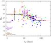 |
Fig. B.1 Relation between the maximum magnitude and the rate of decline for extragalactic novae. The PTF data are shown by red × symbols, WeCAPP – blue stars, Shafter et al. (2011) data – green squares, Capaccioli et al. (1989) data – magenta filled circles, Kasliwal et al. (2011) data – orange open circles, and the purple square is the recurrent nova M 31N 2008-12a in M 31. The black triangles represent the averages in the bins, and the red dotted line is our fit. The line segments on the left side mark the approximate limiting magnitudes of the surveys (as shown by the legend). |
Mean nova peak magnitudes and their standard deviations.
The collected data are shown in Fig. B.1. To quantify the data in a statistical manner, we grouped them according to the decline times, with the bin-width adjusted to have equal number (19) of novae in each bin. For each bin we computed the mean magnitude and its standard deviation (Table B.1), the values of which were fed into our simulations as described in Sect. 4.
As a final word of caution, the data used in computing Table B.1 are collected from a heterogeneous set of magnitude limited surveys. Therefore, our results should not be interpreted as an attempt to produce an updated version of the MMRD relation. Incompleteness of individual surveys could bias our calculations of mean magnitudes, shifting them upward. However, the magnitude limits of the majority of the surveys used here are deep enough (Fig. B.1), therefore our results should be sufficiently accurate for the purpose of the illustrative calculation undertaken here.
It is generally limited by the unresolved surface brightness of the host galaxy rather than the limiting magnitude of the survey as such (see Sect. 4).
Since the red bands contain the H-alpha emission line, which declines more slowly than the continuum, the quoted t2 time may be somewhat overestimated compared to the t2 measured in the V-band (see Darnley et al. 2006). An accurate accounting for this effect is beyond the scope of this paper; we note, however, that it will increase the predicted rates (cf. Fig. 2) and will result in an even tighter constraint.
We recall that in Yaron et al. (2005) models, the t2 ≈ 10 days corresponds to the WD mass of ≈ 1.3M⊙, with the more massive WDs producing faster novae.
In some respect our approach is similar to the one used by Darnley et al. (2006) for their completeness analysis, with the difference that they used the very same novae detected in their survey, whereas here we used average statistical properties of a large compilation of novae.
This estimate is valid for a random observing pattern. For the particular schedule of PTF observations in 2009–2010 shown in Fig. 2 of Cao et al. (2012), this needs to be decreased by a factor of a few because there were extended gaps in the observing schedule; more accurate calculations are beyond the scope of this work.
Acknowledgments
We would like to thank Chien-Hsiu Lee for making available to us the tabulated data of the detected novae from WeCAPP. We are grateful to Pauline Barmby for providing us the Spitzer 3.6 micron mosaic image of M 31. M.G. acknowledges hospitality of the Kazan Federal University (KFU) and support by the Russian Government Program of Competitive Growth of KFU. The authors would like to thank the anonymous referee for the constructive and inspiring comments and suggestions that helped to improve the paper.
References
- Arp, H. C. 1956, AJ, 61, 15 [NASA ADS] [CrossRef] [Google Scholar]
- Barmby, P., Ashby, M. L. N., Bianchi, L., et al. 2006, ApJ, 650, L45 [NASA ADS] [CrossRef] [Google Scholar]
- Barmby, P., Ashby, M. L. N., Bianchi, L., et al. 2007, ApJ, 655, L61 [NASA ADS] [CrossRef] [Google Scholar]
- Battaner, E., Beckman, J. E., Mediavilla, E., et al. 1986, A&A, 161, 70 [NASA ADS] [Google Scholar]
- Bertin, E., & Arnouts, S. 1996, A&AS, 117, 393 [NASA ADS] [CrossRef] [EDP Sciences] [Google Scholar]
- Bildsten, L., Shen, K. J., Weinberg, N. N., & Nelemans, G. 2007, ApJ, 662, L95 [NASA ADS] [CrossRef] [Google Scholar]
- Blanton, M. R., & Roweis, S. 2007, AJ, 133, 734 [NASA ADS] [CrossRef] [Google Scholar]
- Bode, M. F., & Evans, A. 2008, Classical Novae, eds. M. F. Bode, & A. Evans 2nd edn. (Cambridge University Press), Cambridge Astrophys. Ser., 43 [Google Scholar]
- Brown, T. M., Smith, E., Ferguson, H. C., et al. 2006, ApJ, 652, 323 [NASA ADS] [CrossRef] [Google Scholar]
- Cao, Y., Kasliwal, M. M., Neill, J. D., et al. 2012, ApJ, 752, 133 [NASA ADS] [CrossRef] [Google Scholar]
- Capaccioli, M., della Valle, M., Rosino, L., & D’Onofrio, M. 1989, AJ, 97, 1622 [NASA ADS] [CrossRef] [Google Scholar]
- Cassisi, S., Iben, Jr., I., & Tornambe, A. 1998, ApJ, 496, 376 [NASA ADS] [CrossRef] [Google Scholar]
- Darnley, M. J., Bode, M. F., Kerins, E., et al. 2004, MNRAS, 353, 571 [Google Scholar]
- Darnley, M. J., Bode, M. F., Kerins, E., et al. 2006, MNRAS, 369, 257 [NASA ADS] [CrossRef] [Google Scholar]
- Darnley, M. J., Williams, S. C., Bode, M. F., et al. 2014, A&A, 563, L9 [NASA ADS] [CrossRef] [EDP Sciences] [Google Scholar]
- de Vaucouleurs, G., de Vaucouleurs, A., Corwin, Jr., H. G., et al. 1991, Third Reference Catalogue of Bright Galaxies, Vol. I: Explanations and references. Vol. II, Data for galaxies between 0h and 12h, Vol. III, Data for galaxies between 12h and 24h [Google Scholar]
- della Valle, M., & Livio, M. 1995, ApJ, 452, 704 [NASA ADS] [CrossRef] [Google Scholar]
- Devereux, N. A., Price, R., Wells, L. A., & Duric, N. 1994, AJ, 108, 1667 [NASA ADS] [CrossRef] [Google Scholar]
- Downes, R. A., & Duerbeck, H. W. 2000, AJ, 120, 2007 [NASA ADS] [CrossRef] [Google Scholar]
- Fujimoto, M. Y. 1982, ApJ, 257, 767 [NASA ADS] [CrossRef] [Google Scholar]
- Gil-Pons, P., García-Berro, E., José, J., Hernanz, M., & Truran, J. W. 2003, A&A, 407, 1021 [NASA ADS] [CrossRef] [EDP Sciences] [Google Scholar]
- Gilfanov, M., & Bogdán, Á. 2010, Nature, 463, 924 [NASA ADS] [CrossRef] [PubMed] [Google Scholar]
- Gilfanov, M., & Bogdán, Á. 2011, in AIP Conf. Ser. 1379, eds. E. Göğüş, T. Belloni, & Ü. Ertan, 17 [Google Scholar]
- Hachisu, I., & Kato, M. 2001, ApJ, 558, 323 [NASA ADS] [CrossRef] [Google Scholar]
- Hachisu, I., Kato, M., & Nomoto, K. 1996, ApJ, 470, L97 [NASA ADS] [CrossRef] [Google Scholar]
- Henze, M., Ness, J.-U., Darnley, M. J., et al. 2014, A&A, 563, L8 [NASA ADS] [CrossRef] [EDP Sciences] [Google Scholar]
- Hillman, Y., Prialnik, D., Kovetz, A., & Shara, M. M. 2015, MNRAS, 446, 1924 [NASA ADS] [CrossRef] [Google Scholar]
- Howell, S. B. 2006, Handbook of CCD Astronomy, eds. R. Ellis, J. Huchra, S. Kahn, G. Rieke, & P. B. Stetson [Google Scholar]
- Howell, D. A. 2011, Nat. Comm., 2, 350 [Google Scholar]
- Howell, D. A., Sullivan, M., Nugent, P. E., et al. 2006, Nature, 443, 308 [NASA ADS] [CrossRef] [PubMed] [Google Scholar]
- Hubble, E. P. 1929, ApJ, 69, 103 [NASA ADS] [CrossRef] [Google Scholar]
- Iben, Jr., I., & Tutukov, A. V. 1984, ApJS, 54, 335 [NASA ADS] [CrossRef] [Google Scholar]
- Idan, I., Shaviv, N. J., & Shaviv, G. 2013, MNRAS, 433, 2884 [NASA ADS] [CrossRef] [Google Scholar]
- Johansson, J., Woods, T. E., Gilfanov, M., et al. 2014, MNRAS, 442, 1079 [NASA ADS] [CrossRef] [Google Scholar]
- Jordi, K., Grebel, E. K., & Ammon, K. 2006, A&A, 460, 339 [NASA ADS] [CrossRef] [EDP Sciences] [Google Scholar]
- Kahabka, P., & van den Heuvel, E. P. J. 1997, ARA&A, 35, 69 [NASA ADS] [CrossRef] [Google Scholar]
- Kamiya, Y., Tanaka, M., Nomoto, K., et al. 2012, ApJ, 756, 191 [NASA ADS] [CrossRef] [Google Scholar]
- Kasliwal, M. M., Cenko, S. B., Kulkarni, S. R., et al. 2011, ApJ, 735, 94 [NASA ADS] [CrossRef] [Google Scholar]
- Kato, M., Saio, H., Hachisu, I., & Nomoto, K. 2014, ApJ, 793, 136 [NASA ADS] [CrossRef] [Google Scholar]
- Kromer, M., Sim, S. A., Fink, M., et al. 2010, ApJ, 719, 1067 [NASA ADS] [CrossRef] [Google Scholar]
- Laher, R. R., Surace, J., Grillmair, C. J., et al. 2014, PASP, 126, 674 [NASA ADS] [Google Scholar]
- Law, N. M., Kulkarni, S. R., Dekany, R. G., et al. 2009, PASP, 121, 1395 [NASA ADS] [CrossRef] [Google Scholar]
- Lee, C.-H., Riffeser, A., Seitz, S., et al. 2012, A&A, 537, A43 [NASA ADS] [CrossRef] [EDP Sciences] [Google Scholar]
- Li, W., Chornock, R., Leaman, J., et al. 2011, MNRAS, 412, 1473 [NASA ADS] [CrossRef] [Google Scholar]
- Liu, W.-M., Chen, W.-C., Wang, B., & Han, Z. W. 2010, A&A, 523, A3 [NASA ADS] [CrossRef] [EDP Sciences] [Google Scholar]
- Mannucci, F., Della Valle, M., Panagia, N., et al. 2005, A&A, 433, 807 [NASA ADS] [CrossRef] [EDP Sciences] [Google Scholar]
- Maoz, D., & Mannucci, F. 2012, PASA, 29, 447 [NASA ADS] [CrossRef] [Google Scholar]
- Maoz, D., Mannucci, F., & Nelemans, G. 2014, ARA&A, 52, 107 [NASA ADS] [CrossRef] [Google Scholar]
- Mighell, K. J. 1999, in Astronomical Data Analysis Software and Systems VIII, eds. D. M. Mehringer, R. L. Plante, & D. A. Roberts, ASP Conf. Ser., 172, 317 [Google Scholar]
- Milne, P. A., Foley, R. J., Brown, P. J., & Narayan, G. 2015, ApJ, 803, 20 [NASA ADS] [CrossRef] [Google Scholar]
- Nomoto, K. 1982, ApJ, 253, 798 [NASA ADS] [CrossRef] [Google Scholar]
- Nomoto, K., Saio, H., Kato, M., & Hachisu, I. 2007, ApJ, 663, 1269 [NASA ADS] [CrossRef] [Google Scholar]
- Olsen, K. A. G., Blum, R. D., Stephens, A. W., et al. 2006, AJ, 132, 271 [NASA ADS] [CrossRef] [Google Scholar]
- Pagnotta, A., & Schaefer, B. E. 2014, ApJ, 788, 164 [NASA ADS] [CrossRef] [Google Scholar]
- Patat, F., Chugai, N. N., Podsiadlowski, P., et al. 2011, A&A, 530, A63 [NASA ADS] [CrossRef] [EDP Sciences] [Google Scholar]
- Perlmutter, S., Aldering, G., Goldhaber, G., et al. 1999, ApJ, 517, 565 [NASA ADS] [CrossRef] [Google Scholar]
- Pietsch, W., Haberl, F., Sala, G., et al. 2007, A&A, 465, 375 [NASA ADS] [CrossRef] [EDP Sciences] [Google Scholar]
- Prialnik, D., & Kovetz, A. 1995, ApJ, 445, 789 [NASA ADS] [CrossRef] [Google Scholar]
- Riess, A. G., Filippenko, A. V., Challis, P., et al. 1998, AJ, 116, 1009 [NASA ADS] [CrossRef] [Google Scholar]
- Riffeser, A., Fliri, J., Gössl, C. A., et al. 2001, A&A, 379, 362 [NASA ADS] [CrossRef] [EDP Sciences] [Google Scholar]
- Ritter, H., Politano, M., Livio, M., & Webbink, R. F. 1991, ApJ, 376, 177 [NASA ADS] [CrossRef] [Google Scholar]
- Schlegel, D. J., Finkbeiner, D. P., & Davis, M. 1998, ApJ, 500, 525 [NASA ADS] [CrossRef] [Google Scholar]
- Shafter, A. W., Rau, A., Quimby, R. M., et al. 2009, ApJ, 690, 1148 [NASA ADS] [CrossRef] [Google Scholar]
- Shafter, A. W., Darnley, M. J., Hornoch, K., et al. 2011, ApJ, 734, 12 [Google Scholar]
- Shafter, A. W., Hornoch, K., Ciardullo, J. V. R., Darnley, M. J., & Bode, M. F. 2012, The Astronomer’s Telegram, 4503, 1 [NASA ADS] [Google Scholar]
- Shafter, A. W., Curtin, C., Pritchet, C. J., Bode, M. F., & Darnley, M. J. 2014, in Stell Novae: Past and Future Decades, eds. P. A. Woudt, & V. A. R. M. Ribeiro, ASP Conf. Ser., 490, 77 [Google Scholar]
- Shafter, A. W., Henze, M., Rector, T. A., et al. 2015, ApJS, 216, 34 [NASA ADS] [CrossRef] [Google Scholar]
- Shore, S. N., De Gennaro Aquino, I., Schwarz, G. J., et al. 2013, A&A, 553, A123 [NASA ADS] [CrossRef] [EDP Sciences] [Google Scholar]
- Sim, S. A., Röpke, F. K., Hillebrandt, W., et al. 2010, ApJ, 714, L52 [Google Scholar]
- Sokoloski, J. L., Kenyon, S. J., Espey, B. R., et al. 2006, ApJ, 636, 1002 [NASA ADS] [CrossRef] [Google Scholar]
- Starrfield, S. 2014, AIP Adv., 4, 041007 [NASA ADS] [CrossRef] [Google Scholar]
- Starrfield, S., Sparks, W. M., & Truran, J. W. 1985, ApJ, 291, 136 [NASA ADS] [CrossRef] [Google Scholar]
- Strope, R. J., Schaefer, B. E., & Henden, A. A. 2010, AJ, 140, 34 [NASA ADS] [CrossRef] [Google Scholar]
- Sullivan, M., Le Borgne, D., Pritchet, C. J., et al. 2006, ApJ, 648, 868 [NASA ADS] [CrossRef] [Google Scholar]
- Tang, S., Bildsten, L., Wolf, W. M., et al. 2014, ApJ, 786, 61 [NASA ADS] [CrossRef] [Google Scholar]
- Tempel, E., Tuvikene, T., Tamm, A., & Tenjes, P. 2011, A&A, 526, A155 [NASA ADS] [CrossRef] [EDP Sciences] [Google Scholar]
- Totani, T., Morokuma, T., Oda, T., Doi, M., & Yasuda, N. 2008, PASJ, 60, 1327 [NASA ADS] [CrossRef] [Google Scholar]
- Townsley, D. M., & Bildsten, L. 2004, ApJ, 600, 390 [NASA ADS] [CrossRef] [Google Scholar]
- Truran, J. W., & Livio, M. 1986, ApJ, 308, 721 [NASA ADS] [CrossRef] [Google Scholar]
- van den Heuvel, E. P. J., Bhattacharya, D., Nomoto, K., & Rappaport, S. A. 1992, A&A, 262, 97 [NASA ADS] [Google Scholar]
- Vilardell, F., Ribas, I., Jordi, C., Fitzpatrick, E. L., & Guinan, E. F. 2010, A&A, 509, A70 [NASA ADS] [CrossRef] [EDP Sciences] [Google Scholar]
- Walder, R., Folini, D., & Shore, S. N. 2008, A&A, 484, L9 [NASA ADS] [CrossRef] [EDP Sciences] [Google Scholar]
- Wang, B., & Han, Z. 2012, New A Rev., 56, 122 [Google Scholar]
- Webbink, R. F. 1984, ApJ, 277, 355 [NASA ADS] [CrossRef] [Google Scholar]
- Whelan, J., & Iben, Jr., I. 1973, ApJ, 186, 1007 [NASA ADS] [CrossRef] [Google Scholar]
- Wolf, W. M., Bildsten, L., Brooks, J., & Paxton, B. 2013, ApJ, 777, 136 [NASA ADS] [CrossRef] [Google Scholar]
- Wood-Vasey, W. M., & Sokoloski, J. L. 2006, ApJ, 645, L53 [NASA ADS] [CrossRef] [Google Scholar]
- Woods, T. E., & Gilfanov, M. 2013, MNRAS, 432, 1640 [NASA ADS] [CrossRef] [Google Scholar]
- Woods, T. E., & Gilfanov, M. 2014, MNRAS, 439, 2351 [NASA ADS] [CrossRef] [Google Scholar]
- Woosley, S. E., & Weaver, T. A. 1994, ApJ, 423, 371 [NASA ADS] [CrossRef] [Google Scholar]
- Yaron, O., Prialnik, D., Shara, M. M., & Kovetz, A. 2005, ApJ, 623, 398 [NASA ADS] [CrossRef] [Google Scholar]
All Tables
All Figures
|
Fig. 1 Variation of the ignition mass of the nova ΔMign and the mass-loss timescale tml (≈decline time of the outburst by 3 mag from optical peak, t3) with the mass of the WD for the accretion rate Ṁ = 10-7M⊙ yr-1 and WD core temperature 107 K, from Yaron et al. (2005). |
| In the text | |
|
Fig. 2 Cumulative (left) and differential (right) t2 distributions of novae produced by one successful SN Ia progenitor, assuming that it accreted in the unstable nuclear burning regime throughout its entire accretion history. The numbers near the curves indicate the mass-accretion rate. The discontinuities in the differential distributions are caused by the discontinuity in the slope of log-linear interpolation of t2 and MWD values from Yaron et al. (2005) tabulation. They do not affect the cumulative distribution in any significant way, as can be seen in the left panel. The sharp drop in the distributions at low t2 values corresponds to the fastest novae produced by the WD near the Chandrasekhar mass limit. |
| In the text | |
|
Fig. 3 Maximal contribution of novae to the SN Ia rate of M 31 as a function of assumed mass accretion rate for different values of WD core temperature as indicated by the numbers near the curves. The point at Ṁ = 5 × 10⁻⁷M⊙ yr-1 (shown in gray) is computed from the models of Hillman et al. (2015); other points are computed based on Yaron et al. (2005) nova models. The red solid line shows the M 31 supernova rate. |
| In the text | |
|
Fig. 4 Detection efficiency for novae in M 31 as a function of their decline time t2 for surveys with the limiting magnitude of mR = 20 and different temporal sampling (left) and for surveys of different limiting magnitudes with observations performed every night (right). The decline of the detection efficiency for slow novae is caused by their lower peak magnitudes and the finite time span of the simulated survey (see Sect. 4). |
| In the text | |
|
Fig. 5 Fraction of all fast novae with t2 ≤ 10 days detected in surveys of different temporal sampling as a function of their limiting magnitude. It is assumed that the distribution of novae over decay times dnnov(t2)/dt2 is given by Eq. (5)for a mass accretion rate of Ṁ = 10-7M⊙ yr-1. |
| In the text | |
|
Fig. 6 Comparison of the ignition mass of the nova as computed by different authors. The ignition mass is shown as a function of the WD mass for a mass accretion rate Ṁ = 10-7M⊙ yr-1. The Wolf et al. (2013) results are obtained from their Fig. 8; Fujimoto (1982) from their Fig. 7; Starrfield (2014) from their Figs. 2, 3. |
| In the text | |
|
Fig. 7 Comparison of the data shown in Fig. B.1 with the results of multicycle nova models of Yaron et al. (2005). The black triangles and vertical error bars show the average peak magnitudes and their rms deviation for the novae grouped in equipopulated bins over the t2 time, and the curves are corresponding relations for the nova models of Yaron et al. (2005). The red, green and blue curves correspond to WD core temperature of 107 K, 3 × 10⁷ K and 5 × 10⁷ K, respectively. The solid curves are for Ṁ = 10-7M⊙ yr-1, dashed curves for Ṁ = 10-8M⊙ yr-1, short dashed curves for Ṁ = 10-9M⊙ yr-1, dotted curves for Ṁ = 10-10M⊙ yr-1, and dot-dashed curves for Ṁ = 10-11M⊙ yr-1. |
| In the text | |
|
Fig. A.1 Light curves of the sample selected from the S class of the catalog compiled by Strope et al. (2010) with all the peaks aligned at t = 10 days by a linear shift along the time axis (left) and the resulting transformed curves after stretching in time and shifting in magnitude with respect to the reference light curve of V1668 Cyg according to Eq. (A.1)(right). |
| In the text | |
|
Fig. A.2 Co-aligned template light curves from the three nova samples, viz., the Galactic sample from Strope et al. (2010) and the M 31 samples obtained from the WeCAPP and PTF nova catalogs. |
| In the text | |
|
Fig. B.1 Relation between the maximum magnitude and the rate of decline for extragalactic novae. The PTF data are shown by red × symbols, WeCAPP – blue stars, Shafter et al. (2011) data – green squares, Capaccioli et al. (1989) data – magenta filled circles, Kasliwal et al. (2011) data – orange open circles, and the purple square is the recurrent nova M 31N 2008-12a in M 31. The black triangles represent the averages in the bins, and the red dotted line is our fit. The line segments on the left side mark the approximate limiting magnitudes of the surveys (as shown by the legend). |
| In the text | |
Current usage metrics show cumulative count of Article Views (full-text article views including HTML views, PDF and ePub downloads, according to the available data) and Abstracts Views on Vision4Press platform.
Data correspond to usage on the plateform after 2015. The current usage metrics is available 48-96 hours after online publication and is updated daily on week days.
Initial download of the metrics may take a while.