| Issue |
A&A
Volume 583, November 2015
|
|
|---|---|---|
| Article Number | A140 | |
| Number of page(s) | 13 | |
| Section | Stellar structure and evolution | |
| DOI | https://doi.org/10.1051/0004-6361/201424118 | |
| Published online | 05 November 2015 | |
Online material
Appendix A: Nova light-curve template
|
Fig. A.1
Light curves of the sample selected from the S class of the catalog compiled by Strope et al. (2010) with all the peaks aligned at t = 10 days by a linear shift along the time axis (left) and the resulting transformed curves after stretching in time and shifting in magnitude with respect to the reference light curve of V1668 Cyg according to Eq. (A.1)(right). |
|
| Open with DEXTER | |
Nova light curves are known to have a variety of shapes. In an effort to classify them, Strope et al. (2010), using a sample of 93 well-observed Galactic novae, have proposed seven morphological classes. Of these, the smooth (S) class is the most fundamental since the other light-curve shapes can be derived from the smooth class by superposing it with various features. The largest fraction of novae in the sample of Strope et al. (2010; 38%) falls in the S class; more than half of the novae with t3 ≤ 21 days (taking this value to define the fast novae of interest) belong to this class as well. Furthermore, in our simulations, we used light curves within 2−3 mag from the peak, where they generally have a smooth morphology (most of the features defining the distinction between the various classes typically develop much later in time). We thus adopted the S-class light curves to generate the template curve as described below.
We selected all sufficiently well sampled S-class light curves from Strope et al. (2010). In Fig. A.1, these light curves are shown with their peaks aligned by shifting linearly along the time axis. We then used the following transformation to match the light curves: ![]() (A.1)where m(t) is the magnitude in the frame t, m′(t′) is that in the transformed frame t′ = (t−tp)s, tp is the time of the peak of the light curve, Δm the magnitude shift, and s the time stretch factor.
(A.1)where m(t) is the magnitude in the frame t, m′(t′) is that in the transformed frame t′ = (t−tp)s, tp is the time of the peak of the light curve, Δm the magnitude shift, and s the time stretch factor.
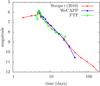 |
Fig. A.2
Co-aligned template light curves from the three nova samples, viz., the Galactic sample from Strope et al. (2010) and the M 31 samples obtained from the WeCAPP and PTF nova catalogs. |
| Open with DEXTER | |
The light curves were transformed to match the reference light curve, for which we chose V1668 Cyg. To this end, we binned the light curves logarithmically (typically five bins or more per dex along the time axis) and determined the magnitude in each bin by taking the average, weighted by the inverse square of the uncertainty in the individual magnitude measurement. The best-fit parameters Δm and s of the transformation Eq. (A.1)were determined by minimizing the χ2. The result of this procedure is shown in the right panel in Fig. A.1. In all cases we were able to obtain a reasonably good agreement, with the values of the stretch factor ranging from ≈ 0.5−2 and the rms dispersion between the reference and individual lightcurves calculated down to 6 mag from the peak being in the range 0.18–0.33 mag. Finally, we averaged the resulting transformed curves by binning in time (logarithmically again) and weighting by the respective uncertainties to produce the template curve.
This template light curve was generated using a Galactic nova sample. Although we do not expect any significant difference from the M 31 novae, for a consistency check we compared our template with light curves from two different M 31 nova samples. We applied the procedure described above to the selection of well-sampled light curves from the nova catalog of the WeCAPP (Riffeser et al. 2001), which have been classified as having smooth morphology (Lee et al. 2012), and to light curves from the PTF M 31 survey in Cao et al. (2012). In these two cases, we were also able to obtain good light curve matches, with the rms dispersion (calculated down to 4 mag from peak) lower than ≈ 0.30 mag. Final template curves were generated using the same procedure as before. The resulting templates are shown in Fig. A.2 along with our default template based on Strope et al. (2010) data. The plot shows that all three templates agree very well with each other. For our calculations, we used the template obtained based on the Strope et al. (2010) data because it is the best sampled and covers the broadest magnitude range.
Appendix B: Peak magnitudes of novae
For each simulated nova we need to assign some value for its peak magnitude. To this end, we produced an analog of the MMRD relation with the caveats detailed below. Various forms of this relation have been obtained previously (for example, see della Valle & Livio 1995; Downes & Duerbeck 2000; Darnley et al. 2006; Shafter et al. 2011), although recently its existence has been questioned (Kasliwal et al. 2011). However, for the purpose of this study, we are not concerned with the existence of the MMRD relation, instead we need to account for the full range of observed nova peak magnitudes in our simulations. We therefore collected a large sample of novae and determined their mean magnitudes and rms scatter in broad bins over t2 as explained below.
We used the light curves from the PTF (Cao et al. 2012) and WeCAPP (Lee et al. 2012) nova catalogs with morphological classification available, the light curves from Shafter et al. (2011) that have been observed in the V-band, the high-quality light curves from Capaccioli et al. (1989), and the sample of extragalactic novae discovered by P60-FasTING (Kasliwal et al. 2011). To this compilation, we added the recently discovered very fast recurrent nova M 31N 2008-12a in M 31 with the shortest known recurrence period of ~ 1 yr (Shafter et al. 2012; Darnley et al. 2014; Henze et al. 2014; Tang et al. 2014). The PTF and WeCAPP light curves were converted from R-band to V-band using the color (V−R)° = 0.16 (Shafter et al. 2009) after accounting for the foreground extinction of AR = 0.15 (Shafter et al. 2009) estimated using a reddening of E(B−V) = 0.062 along the line of sight to M 31 from Schlegel et al. (1998). The light curves from Capaccioli et al. (1989) were corrected for foreground extinction using Apg = 0.25 (Shafter et al. 2009) and converted from the photographic band to V-band using the colors (B−mpg)° = 0.17 (Capaccioli et al. 1989; Arp 1956) and (B−V)° = 0.15 (Shafter et al. 2009). The Kasliwal et al. (2011) light curves were converted from g-band to V-band using the transformation relation from Jordi et al. (2006). Apparent magnitudes were converted to absolute magnitudes using a distance modulus of 24.36 for M 31 (Vilardell et al. 2010). Light curves from Shafter et al. (2011) were corrected for extinction and converted to absolute magnitude in the original publication. Except for the WeCAPP sample, we used the light-curve decline times (t2) from the respective publications. For those novae in Kasliwal et al. (2011) whose t2 times are not available, we approximated them by multiplying the decline times t1 in their Table 5 by two. For the WeCAPP light curves we estimated their decline times ourselves by linearly interpolating between consecutive measurements.
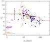 |
Fig. B.1
Relation between the maximum magnitude and the rate of decline for extragalactic novae. The PTF data are shown by red × symbols, WeCAPP – blue stars, Shafter et al. (2011) data – green squares, Capaccioli et al. (1989) data – magenta filled circles, Kasliwal et al. (2011) data – orange open circles, and the purple square is the recurrent nova M 31N 2008-12a in M 31. The black triangles represent the averages in the bins, and the red dotted line is our fit. The line segments on the left side mark the approximate limiting magnitudes of the surveys (as shown by the legend). |
| Open with DEXTER | |
Mean nova peak magnitudes and their standard deviations.
The collected data are shown in Fig. B.1. To quantify the data in a statistical manner, we grouped them according to the decline times, with the bin-width adjusted to have equal number (19) of novae in each bin. For each bin we computed the mean magnitude and its standard deviation (Table B.1), the values of which were fed into our simulations as described in Sect. 4.
As a final word of caution, the data used in computing Table B.1 are collected from a heterogeneous set of magnitude limited surveys. Therefore, our results should not be interpreted as an attempt to produce an updated version of the MMRD relation. Incompleteness of individual surveys could bias our calculations of mean magnitudes, shifting them upward. However, the magnitude limits of the majority of the surveys used here are deep enough (Fig. B.1), therefore our results should be sufficiently accurate for the purpose of the illustrative calculation undertaken here.
© ESO, 2015
Current usage metrics show cumulative count of Article Views (full-text article views including HTML views, PDF and ePub downloads, according to the available data) and Abstracts Views on Vision4Press platform.
Data correspond to usage on the plateform after 2015. The current usage metrics is available 48-96 hours after online publication and is updated daily on week days.
Initial download of the metrics may take a while.