| Issue |
A&A
Volume 581, September 2015
|
|
|---|---|---|
| Article Number | A5 | |
| Number of page(s) | 14 | |
| Section | Galactic structure, stellar clusters and populations | |
| DOI | https://doi.org/10.1051/0004-6361/201322787 | |
| Published online | 21 August 2015 | |
Star formation in the filament of S254-S258 OB complex: a cluster in the process of being created
1
Aix-Marseille Université, CNRS, LAM (Laboratoire d’Astrophysique de
Marseille), UMR 7326,
13388
Marseille,
France
e-mail:
This email address is being protected from spambots. You need JavaScript enabled to view it.
2
Tata Institute of Fundamental Research,
400 005
Mumbai,
India
3
Kavli Institute for Astronomy and Astrophysics, Peking
University, Haidian,
100871
Beijing, PR
China
4
Joint ALMA Observatory, Alonso de Córdova 3107, Vitacura, Santiago, Chile
5
Steward Observatory, University of Arizona,
933 North Cherry Avenue,
Tucson, AZ
85721-0065,
USA
6
Institute of Astronomy, National Central University,
32054
Chung-Li,
Taiwan
7
Aryabhatta Research Institute of Observational Sciences
(ARIES), Manora
Peak, 263129
Nainital,
India
8
Institute of Applied Physics of the Russian Academy of
Sciences, 46 Ulyanov
St., 603950
Nizhny Novgorod,
Russia
9
Lobachevsky State University of Nizhni Novgorod,
23 Gagarin Av., 603950
Nizhny Novgorod,
Russia
10
National Astronomical Observatory of Japan,
Mitaka, 181-8588
Tokyo,
Japan
11
National Centre for Radio Astrophysics, Tata Institute of
Fundamental Research, 411007
Pune,
India
Received: 3 October 2013
Accepted: 30 March 2015
Abstract
Infrared dark clouds are ideal laboratories for studying the initial processes of high-mass star and star-cluster formation. We investigated the star formation activity of an unexplored filamentary dark cloud (size ~5.7 pc × 1.9 pc), which itself is part of a large filament (~20 pc) located in the S254-S258 OB complex at a distance of 2.5 kpc. Using Multi-band Imaging Photometer (MIPS) Spitzer 24 μm data, we uncovered 49 sources with signal-to-noise ratios greater than 5. We identified 45 sources as candidate young stellar objects (YSOs) of Class I, flat-spectrum, and Class II natures. Additional 17 candidate YSOs (9 Class I and 8 Class II) are also identified using JHK and Wide-field Infrared Survey Explorer (WISE) photometry. We find that the protostar-to-Class II sources ratio (~2) and the protostar fraction (~70%) of the region are high. Comparison of the protostar fraction to other young clusters suggests that the star formation in the dark cloud possibly started only 1 Myr ago. Combining the near-infrared photometry of the YSO candidates with the theoretical evolutionary models, we infer that most of the candidate YSOs formed in the dark cloud are low-mass (<2 M⊙). We examine the spatial distribution of the YSOs and find that majority of them are linearly aligned along the highest column density line (N(H2)~1 × 1022 cm-2) of the dark cloud along its long axis at the mean nearest-neighbour separation of ~0.2 pc. Using the observed properties of the YSOs, physical conditions of the cloud and a simple cylindrical model, we explore the possible star formation process of this filamentary dark cloud and suggest that gravitational fragmentation within the filament should have played a dominant role in the formation of the YSOs. From the total mass of the YSOs, the gaseous mass associated with the dark cloud, and the surrounding environment, we infer that the region is presently forming stars at an efficiency of ~3% and a rate ~30 M⊙ Myr-1, and it may emerge in a richer cluster.
Key words: stars: formation / infrared: stars / stars: pre-main sequence / techniques: photometric / HII regions / ISM: clouds
© ESO, 2015
1. Introduction
Recently, filaments and infrared dark clouds (IRDCs) have received special attention because they are the potential progenitors of cluster formation (e.g., Rathborne et al. 2006; Beuther & Sridharan 2007; Peretto & Fuller 2009; Myers 2009; Henning et al. 2010; Battersby et al. 2011; Ragan et al. 2012; Longmore et al. 2012; Russeil et al. 2013). Results from the Herschel Space Telescope, particularly the Gould Belt (André et al. 2010) and Hi-GAL (Molinari et al. 2010) Legacy Surveys, have also emphasized the crucial role of filamentary structures on star and cluster formation. However, due to the complex nature of the interstellar medium (ISM), the modes of fragmentation and the physical processes that govern star formation in filaments are still under active discussion (e.g., Heitsch et al. 2009; Vázquez-Semadeni et al. 2009; Pon et al. 2011; André 2013; Smith et al. 2014). Identifying and characterizing young protostars are the key to partly answering some of these questions, because they still bear the imprint of the fragmentation of the primordial cloud. However, filaments and IRDCs are characterized by high column densities, therefore identifying of such sources is often difficult. In the past decade, observations at longer infrared wavelengths with Mid-infrared Imaging Photometer (MIPS; Carey et al. 2009) and Wide-field Infrared Survey Explorer (WISE; Wright et al. 2010) allowed us to overcome the high extinction in these regions and explore the properties and distribution of associated young sources. In this context, we present an investigation of a filamentary dark cloud located in the S254-S258 OB complex.
The S254-S258 complex, situated at a distance of 2.5 kpc, is part of the Gemini OB association (Chavarría et al. 2008; Bieging et al. 2009; Ojha et al. 2011). The complex contains six H ii regions (S254, S255, S256, S257, S258 and S255B) projected on or in the close vicinity of a long (~20 pc) filamentary cloud (see Fig. 1). The search for young stellar objects (YSOs) in the complex was carried out by Chavarría et al. (2008), Ojha et al. (2011), and Mucciarelli et al. (2011), but these studies mainly focus on the central part of the complex, which roughly cover ≤13 square arcmin area around the massive young cluster S255-IR (Wang et al. 2011; Ojha et al. 2011; Zinchenko et al. 2012) located between the two evolved H ii regions S255 and S257. These studies have shown that the S254-S258 complex contains a rich population of Class I, Class II, Class III, and near-infrared (NIR)-excess sources formed in groups, and also in distributed modes across the complex.
The present study focuses on the star formation activity of a part of the long filament (centered at α2000 = 06h13m47s, δ2000 = 17°54′37′′ or  ,
,  ). The filamentary area under investigation is ~5.7 pc in length and 1.9 pc in width. The region is highly obscured in the optical wavelength regime, and it corresponds to a dense part of the long filament. The region is dense as revealed by the presence of CS (J = 2−1) emission, which is a tracer of dense (>104 cm-3) gas. The distribution of CS emission (see Fig. 4 of Carpenter et al. 1995) is also seen elongated in shape (size ~5.6 pc × 1.7 pc), with long axis along the long axis of the large filament. IRDCs are dense molecular clouds seen as extinction features against the bright background. Molecular line and dust continuum studies of IRDCs have shown that they are cold (T< 25 K), dense (N(H2) ≳ 1022 cm-2), and massive (~102−105M⊙) structures with sizes 1−15 pc (Carey et al. 1998; Simon et al. 2006). Like other IRDCs (e.g., Simon et al. 2006), the area under investigation is dark in the optical (e.g., in DSS2 Survey images) and in the mid-infrared (e.g., in MSX Survey images; Price et al. 2001), and also cold (T ≤ 15 K) and dense (N(H2) ~ 1022 cm-2) in nature (discussed in Sects. 3.5 and 4.2). Following the general nomenclature of the IRDCs (Rathborne et al. 2006; Peretto & Fuller 2009), we hereafter designate the dense cloud under investigation as “IRDC G192.76+00.10”.
Massive OB2 stars ionize the surrounding ISM and create H ii region. During expansion, the H II region drives the shock front that precedes the ionization front. The shock front sweeps up the ISM to form a cold dense shell and star formation can be induced by the instability of the shell (e.g., “collect and collapse” scenario; Elmegreen & Lada 1977). In the S254-S258 complex, Ojha et al. (2011) and Mucciarelli et al. (2011) suggest that there is induced second-generation star formation at the peripheries of S255 and S257. Similar to here, evidence of second-generation triggered star formations have been observed at the peripheries of several H ii regions (e.g., Zavagno et al. 2007; Indebetouw et al. 2007; Chu & Gruendl 2008; Chen et al. 2011; Brand et al. 2011; Deharveng et al. 2012; Getman et al. 2012; Jose et al. 2013; Samal et al. 2014), suggesting that the presence of an H ii region can influence star formation processes of a complex. However, in the S254-S258 complex, the IRDC G192.76+00.10 region is relatively isolated from the feedback effects, because it is situated farther from the known evolved H ii regions (e.g., S254, S255, and S257). Moreover, shell-like filamentary structures resulted from sweeping, and the compression of expanding H ii regions are generally located parallel to the H ii region’s ionization front (e.g., Deharveng et al. 2010; Jose et al. 2013), whereas the filament axis of the IRDC G192.76+00.10 region is perpendicular to the ionization front of the evolved H ii regions of the complex. Also the IRDC G192.76+00.10 area does not seem to be contaminated by polycyclic aromatic hydrocarbon (PAH) emissions at 11.3 μm and 12.7 μm of WISE 12 μm band (not shown), and PAH emissions are generally found at the interaction zone of H ii region and molecular cloud (e.g., Samal et al. 2007; Deharveng et al. 2010). This evidence suggests that the star formation in the IRDC G192.76+00.10 region is unlikely to be influenced by the evolved H ii regions of the complex.
Star formation in the IRDC G192.76+00.10 region has so far not been explored, and were only partly covered by Chavarría et al. (2008) at Spitzer-IRAC wavelengths (i.e., 3.6−8.0 μm) in their YSO search. In the present work, along with 13CO data, we make use of MIPS, WISE, and NIR-JHK band data sets to study the star formation activity of IRDC G192.76+00.10. We present our work with the following layout. We describe the observations and data reduction techniques in Sect. 2. In Sect. 3, the observational results are presented, which include the morphology of the region and identification, distribution, and characterization of YSOs. We discuss the properties and star formation processes of the IRDC G192.76+00.10 cloud and its overall relation with the main filament in Sect. 4.
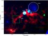 |
Fig. 1 Colour composite image of the complex obtained using the 13CO (110 GHz) column density map in red (from Chavarría et al. 2008), radio emission in green (from NVSS survey at 1.4 GHz; Condon et al. 1998) and optical emission in blue (from DSS2 survey). The abscissa (RA) and ordinate (Dec) are in the J2000 epoch. North is up and east is left. The H ii regions discussed in the text are marked in white circles. The rectangular box represents the area studied in this work (the corresponding image at 24 μm is shown in Fig. 2). |
2. Observations and data reduction
The 24 μm observations of the IRDC G192.76+00.10 region were downloaded from the Spitzer archive (Programme ID 20635), and cover an area ~7.́0 × 8′0, centred at α2000 = 06h13m47s, δ2000 = 17°53′40′′. We downloaded the corrected basic-calibrated data (CBCD) images and the corresponding uncertainty files and then performed source detection and photometry using the MOPEX/APEX software. To extract the flux, we applied the APEX point-response function (PRF) fitting method to the detected sources. We used the zero-point value of 7.17 Jy from the MIPS Data Handbook to convert flux densities to magnitudes. We considered only those 49 sources whose signal-to-noise ratio (S/N) was found to be greater than 5. The magnitudes of these 49 sources along with their corresponding uncertainties are given in Table 1. We point out that the reported uncertainties are lower limits to the actual values, since the uncertainty in the absolute flux densities at 24 μm is ~4% (Engelbracht et al. 2007).
We also downloaded MIPS 70 μm CBCD image from the Spitzer archive (Programme ID 20635), and performed photometry using APEX-PRF fitting method as discussed above. The area covered by the MIPS 70 μm image is ~5.́7 × 2.́0, centred at α2000 = 06h13m47s, δ2000 = 17°54′45′′. We detected only four point sources with S/N> 5. The zero-point value of 0.778 Jy, adopted from the MIPS Data Handbook, was used to convert the PRF fitted flux densities of these sources to magnitudes.
Deep NIR observations of the IRDC G192.76+00.10 region in J (λ = 1.25μm), H (λ = 1.63μm), and K (λ = 2.14μm) bands were obtained from the WFCAM Science Archive (Hambly et al. 2008), taken with the WFCAM instrument (Casali et al. 2007) at the United Kingdom Infrared Telescope (UKIRT). We performed photometry on the retrieved stacked images produced by the WFCAM pipeline at the Cambridge Astronomical Survey Unit (CASU) for an area of ~15 × 12 around the IRDC region centred at α2000 = 06h13m48s and δ2000 = 17°52′50′′. Photometry on the images was done using the PSF algorithm of DAOPHOT package (Stetson 1987) in IRAF. The PSF was determined from the bright and isolated stars of the field. For photometric calibration, we used isolated Two Micron All Sky Survey (2MASS) point sources (Cutri et al. 2003) having error <0.1 mag and rd-flag “123”. Rd-flag values of “1”, “2”, or “3” generally indicate the best-quality detections, photometry and astrometry, respectively. A mean calibration dispersion of ≤0.07 mag is observed in each band, indicating that our photometry is reliable within ~0.07 mag. Saturated sources in our catalogue were replaced by 2MASS sources.
Only 9 out of the 49 MIPS detected sources have a counterpart in the NIR and Spitzer-IRAC bands from the catalogue of Chavarría et al. (2008). We thus mostly used WISE and our NIR point source catalogues to classify YSOs and to construct their spectral energy distributions (SEDs). The WISE survey (Cutri et al. 2012) provides photometry at four wavelengths: 3.4, 4.6, 12 and 22 μm, with angular resolutions of 6.̋1, 6.̋4, 6.̋5 and 12.̋0, respectively. We merged the MIPS catalogue with the WISE and NIR catalogues using a matching radius of 3.̋0 (following Koenig et al. 2012).
Chavarría et al. (2008) have observed the complex in the J = 1−0 spectral lines of 12CO and 13CO using the Five College Radio Astronomy Observatory (FCRAO) 14 m telescope. The FCRAO beam size is 45′′ in 12CO and 46′′ in 13CO . We used the 13CO column density map of Chavarría et al. (2008) to study the gas content of the region.
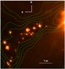 |
Fig. 2 Spitzer MIPS 24 μm image of IRDC G192.76+00.10. The image has a field of view ~7.́0 × 8.́0 centred at α2000 = 06h13m47s, δ2000 = 17°54′37′′ or |

3. Results
3.1. Morphology
The MIPS 24 μm image of the IRDC G192.76+00.10 region is shown in Fig. 2. The image displays a significant number of point-like sources aligned roughly in a linear sequence from south-east to north-west, and most of the point sources seem to be bounded by an elongated structure of 13CO gas. Since dark cloud and dense molecular gas are the sites of new star formation, these sources are possibly young protostars in their early evolutionary stages. To study the star formation activity of the region, it is necessary to characterize and discuss the nature of these sources.
3.2. Identification of young stellar objects
The circumstellar dust emission from the disk and infalling envelope of young stars gradually disappears with time as a function of their evolutionary phases. A number of classification methods are employed in the literature to classify evolutionary phases of YSOs; often used are the near- to mid-infrared spectral index α (Lada 1987), the ratio of submillimetre to bolometric luminosity Lsubmm/Lbol (e.g., André et al. 2000), and the bolometric temperature Tbol (e.g., Myers et al. 1998). Generally, submillimetre luminosity is taken to be the integrated luminosity at wavelengths λ ≥ 350μm. The bolometric luminosity is calculated by integrating the SED over extensive wavelength coverage, covering the far-infrared and millimetre domains. Similarly, the bolometric temperature is defined as the temperature of a black body with the same mean frequency as the source SED over a wide wavelength coverage. Since, the identified point sources typically have flux measurements at λ< 24 μm, accurate determinations of Lbol, Tbol, and Lsubmm are not feasible with the data; thus, in this work, we classified the sources based on their α values.
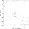 |
Fig. 3 [3.4]−[24] vs. [3.4] colour-magnitude diagram for the detected MIPS 24 μm sources. The dotted lines separate the regions of Class I, flat-spectrum, Class II, and Class III objects. The dashed lines denote the dividing line between the region occupied by contaminated sources (galaxies and diskless stars) and YSOs (see also Rebull et al. 2011). The sources for which we do not have WISE 3.4 μm detection are represented in red. For these sources, we consider the magnitude of the faintest 3.4 μm counterpart of our 24 μm detections as an upper-limit. The arrow represents the direction of their colours, they are likely to be Class I YSOs. |
Out of the 49 MIPS detections (see Sect. 2), 38 have WISE counterparts in all four WISE bands. We estimated spectral index (α = dlog (λFλ) / dlog (λ), where Fλ is the flux as a function of wavelength, λ) for these 38 sources from a linear fit to the fluxes in the range 3.4 to 24 μm (four WISE bands and MIPS 24 μm band), and then classified sources as Class I (α ≥ 0.3), flat-spectrum (0.3 >α ≥ −0.3), Class II (−0.3 >α ≥ −1.6), and Class III (α< −1.6) YSOs following Evans et al. (2009). Using the above approach, we find that out of the 38 sources, 16, 7, 11, and 4 sources are Class I, flat-spectrum, Class II, and Class III YSOs, respectively. The α values of the 38 sources are also tabulated in Table 1. Here we would like to mention that, though α is one of the most commonly used methods for classifying YSOs, it is highly susceptible to disk geometry and source inclination (e.g., Robitaille et al. 2006; Crapsi et al. 2008a). Also in this approach the distinction of the Class 0 YSOs from the Class I is not possible because no well-defined α criteria exist for Class 0 sources. This is because the Class 0 spectrum has the lowest flux densities from 1.25−24 μm as expected for deeply embedded sources with massive, extincting envelopes, thus were largely not identified in the mid-IR prior to Spitzer. However, it is possible to distinguish them from the Class I sources based on their Lsubmm/Lbol and Tbol estimations as discussed in André et al. (2000) and Myers et al. (1998).
It has been found that a strong correlation between the colour and spectral index exists, which provides an acceptable proxy for classifying YSOs (see, e.g., Rebull et al. 2007, 2010). We used the [3.4] vs. [3.4]−[24] colour–magnitude diagram (see Fig. 3) to classify YSOs (Guieu et al. 2010). In Fig. 3, the regions occupied by Class III/main-sequence (MS), Class II, Flat-spectrum, and Class I objects are indicated. In this diagram, 34 sources are located in the regions occupied by Class I, Flat-spectrum, and Class II YSOs, whereas four sources are found in the zone of diskless stars. We confirmed the nature of these four sources as diskless stars with SED modelling (see Sect. 3.6); these sources will not be considered as YSOs in the following. For 11 MIPS detections, 3.4 μm counterparts are not available. For these sources we then considered the magnitude of the faintest 3.4 μm counterpart of the 24 μm detections as an upper limit, in order to determine their positions on the [3.4] vs. [3.4]−[24] diagram. The approximate positions of these 11 sources are shown in Fig. 3, and they appear to be Class I YSOs. Out of these 11 sources, four have a K-band detection. We find that they also fall in the Class I zone in the K vs. K − [ 24 ] diagram (e.g., Rebull et al. 2007), suggesting that these sources are likely to be Class I YSOs. For four Class I YSOs, we have 70 μm flux, so we used the [24] vs. [24]−[70] diagram (e.g., Rebull et al. 2007) to be more precise about their nature; their positions on the [24] vs. [24]−[70] diagram suggest that they are indeed Class I YSOs.
MIPS 24 μm photometry for the 49 sources detected in the IRDC G192.76+00.10 region with a S/N greater than 5.
In Fig. 3, most of the sources have [3.4]−[24] colour >4. A normal MS star has [3.4]−[24] colour around 0.0. Thus, a normal MS star would require a foreground visual extinction (AV ) of ~210 mag to redden up to the location [3.4]−[24] ~ 4, whereas the mean AV of the region is ~10 mag (see Sect. 3.3), suggesting that most of the MIPS sources are most likely YSOs with disks and/or envelopes. However, the YSO sample can be contaminated by background dusty active galactic nuclei (AGN) and star-forming galaxies, since they have colours similar to YSOs. As a result, in Fig. 3, we marked the approximate zones of such sources based on the Spitzer Wide-area Infrared Extra-galactic Survey catalogue (Rowan-Robinson et al. 2008) observations of the ELAIS N1 extra-galactic field. Two sources of our sample (i.e., sources with [3.4]−[24] colour between 6 and 7 mag) fall in the extra-galactic zone. However, these sources are found close to other YSO candidates and are likely members. Similar to galaxies, the colours of the asymptotic giant branch (AGB) stars can also mimic the colour of YSOs. AGB stars show a steep spectral index at long wavelengths. Based on their SEDs, Robitaille et al. (2008) used a criterion [8.0]−[24] < 2.5 to identify them. In the absence of IRAC 8.0 μm data, we are unable to apply Robitaille et al. (2008) criteria to eliminate such sources. However, based on AGB stars distribution, Robitaille et al. (2008) establish an empirical relationship that roughly reflects the expected number of AGB stars per square degree area on the sky for a given Galactic longitude and latitude. Using the Robitaille et al. (2008) relationship, we calculated that the AGB star contamination to our YSO sample is likely to be less than one.
The above discussions suggest that the contamination of non-YSO sources to our MIPS identified YSO sample should be negligible. We therefore considered all the 45 MIPS identified YSO candidates of different classes (27 Class I, 7 Flat-spectrum, and 11 Class II) for further analyses.
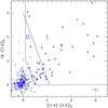 |
Fig. 4 Intrinsic K − [ 3.4 ] vs. [3.4]−[4.6] colour–colour diagram showing the distribution of field stars/MS sources (cross symbols), Class II YSOs (blue stars) and Class I YSOs (red stars). The slanted line indicates the boundary between the Class I and Class II YSOs. The control field sources are indicated by open circles. The error bars in the bottom right corner show average errors in the colours. |
3.3. Additional YSO candidates
The YSO detection using the above method is primarily limited by the 24 μm detection limit. Thus, we may be missing faint YSOs of the region. To overcome this problem, we matched the WISE catalogue to our K-band point-source catalogue, and then selected YSO candidates using the intrinsic K–[3.4] vs. [3.4]−[4.6] colour–colour diagram as suggested by Koenig et al. (2012). The intrinsic K–[3.4] vs. [3.4]−[4.6] diagram is shown in Fig. 4, and the zones of Class II and Class I YSOs are also marked. To construct intrinsic colour–colour diagram, we measured the visual extinction towards individual YSOs from the H2 column density map (see Sect. 3.5), and then used extinction laws of Bohlin et al. (1978) and Flaherty et al. (2007) to compute their dereddened K–[3.4] and [3.4]−[4.6] colours. We then used Koenig et al. (2012) criterion to select the Class I and Class II YSOs from the intrinsic K–[3.4] vs. [3.4]−[4.6] diagram. This helped us to identify 17 additional YSO candidates, which include 8 Class II and 9 Class I YSOs. To quantify the contamination of other sources to this selection, we selected a control field devoid of CO gas and located outside the filamentary area, but within the field of view of our NIR observations. We then looked for the distribution of control field sources on K–[3.4] vs. [3.4]−[4.6] diagram. These sources are also shown in Fig. 4. Their distributions suggest that the majority of them are field stars, indicating that the contamination of other sources to the YSOs sample, selected based on a K–[3.4] vs. [3.4]−[4.6] diagram, should only be a few.
In summary, we have identified 62 YSO candidates in the IRDC G192.76+00.10 region with excess IR emission. Of these, 43 have excess consistent with Class I plus flat-spectrum YSOs, and 19 have excess consistent with Class II YSOs. We note that even though the near-to-mid-infrared colours are very useful for identifying YSOs, the YSO selection and classification can be biased due to disk geometry and/or source inclination along the line of sight. Infrared spectroscopic observations provide many useful indicators that are helpful for the YSO confirmation and disentanglement of deeply embedded protostars from the evolved YSOs (e.g., Reach 2007; Spezzi et al. 2008; Crapsi et al. 2008b; Connelley & Greene 2010); however, foreground absorption and edge-on disks can still confuse the YSO classification (e.g., Pontoppidan et al. 2005). Nevertheless, it has been found that the YSO selection scheme based on photometric colours provides a good representation of YSOs identification in star-forming complexes. As an example, Spezzi et al. (2008) with spectroscopic study of Chameleon II cloud found that 96% of the YSOs identified in Spitzer c2d Legacy survey (Evans et al. 2003) using photometric colours were true members.
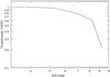 |
Fig. 5 Completeness of the 24 μm band data for the IRDC G192.76+00.10 region from artificial star experiment. |
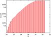 |
Fig. 6 Cumulative distribution of all the K-band sources observed towards the IRDC G192.76+00.10 region. |
3.4. Completeness limit
The identification of YSOs in a star-forming region using multi-band data sets is a strong function of the band-pass sensitivities and extinction of the star-forming region. Our primary criterion for selecting YSOs in the present work is the detection in MIPS 24 μm band. Although the 5σ detection limit of our 24 μm catalog is ~9.6 mag, the completeness limit of the catalog is ~6.7 mag. We calculated completeness limit of our 24 μm catalogue using artificial star experiments. In this approach, we insert artificial stars of different magnitudes to the 24 μm image and then perform their detection and phototmetry to recover them. Figure 5 shows the completeness fraction of artificial stars versus corresponding 24 μm magnitudes. This suggests that our 24 μm detection is 80% complete up to ~6.7 mag. Using SED models of Robitaille et al. (2007), we roughly estimated that our 24 μm data is actually more complete towards the high-mass ends. The additional YSOs obtained using the K–[3.4] vs. [3.4]−[4.6] colour–colour diagram helped us to recover fainter YSOs. The WISE catalogue is 95% complete at [3.4] = 16.9 mag and [4.6] = 15.5 mag (Cutri et al. 2012). We found that 90% of the 3.4 μm and 4.6 μm sources have a K-band counterpart, thus the majority of the WISE sources have been detected in our K band. We estimated the completeness limit of our K-band catalogue by measuring the magnitude at which the cumulative logarithmic distribution of sources as a function of magnitude departs from a linear slope and begins to turn over. Based on this distribution (see Fig. 6), our K-band catalogue turned out to be largely complete down to K ~ 16.5 mag. We tested this approach to our 24 μm detections, and the resulting completeness limit turns out to be ~7 mag, comparable to the completeness limit found using the artificial star experiment.
One of the important properties of YSOs is the intrinsic luminosity. Because of the extinction and/or youthfulness of the sources, we detected only ~50% of the total YSOs in the J band in comparison to the K band. We thus used K-band magnitudes to estimate the luminosities of the YSOs. The K band can be affected by the excess emission from the circumstellar material. To account for this excess emission, we used average excess emission in the K band found in T-Tauri stars. Meyer et al. (1997) found that T-Tauri stars typically have a K-band excess between 0.1 and 1.1 mag, with a median value ~0.6 mag. Considering 0.6 mag as the excess emission at the K band for all our YSOs and using the evolutionary model of Baraffe et al. (2003) for an age of 1 Myr (see Sect. 4.1) at 2.5 kpc and at AV~10 mag, we estimated that our K-band completeness level (i.e., K ~ 16.5 mag) corresponds to a 0.14 L⊙ or 0.15 M⊙ star. Thus, our YSO sample is expected to be largely complete above 0.14 L⊙ or 0.15 M⊙. However, for very low-mass stars the adopted excess emission value of 0.6 mag may not be valid, because in the substellar regime, the inner part of these disks might not emit significant excess emission in the K band. Thus, if we consider the emission in the K band is only from stellar photospheres for low-mass YSOs, our completeness limit would be ~0.2 L⊙ or 0.2 M⊙.
It is difficult to derive the true intrinsic luminosities of YSOs without spectroscopic observations. Therefore in the absence of short-wavelength fluxes or spectroscopic observations, the above approach appears to be reasonable for having the approximate luminosity (or mass) of these objects. Since the effect of excess emission in the J band is minimum, we also estimated the masses of YSOs using J-band magnitudes. For sources detected in both the J and K bands, we found that, for the majority of our YSOs, the difference in mass estimations is within ~40%. Considering tentatively that this is the uncertainty associated in the mass estimations, the absolute K-band magnitudes of the majority of the YSO candidates suggest that the region is mainly composed of low-mass (<2 M⊙) YSOs with a mean mass ~0.3 M⊙.
For the IRDC G192.76+00.10 region, the IRAC four-band data sets are unavailable. Thus to quantify the extra percentage of Class II and Class I YSOs, we might have detected if the IRAC observation had been performed, we analysed a nearby cloud “G192.75-0.08”. The G192.75-0.08 cloud is located within the S254-S258 complex and has been studied by Chavarría et al. (2008) in the IRAC bands. We chose the G192.75-0.08 cloud because it is devoid of bright PAH emission like the IRDC G192.76+00.10 region, and also at comparable extinction. To compare, we first selected YSOs of the G192.75-0.08 region using the [3.4] vs. [3.4]−[24] diagram as described in Sect. 3.3 and then compared the statistics with the YSOs identified by Chavarría et al. (2008). We considered only those YSOs from the Chavarría et al. (2008) catalogue whose spectral index is greater than −1.6, as done in the present work. This statistical comparison indicates that if IRAC observations had been performed for the IRDC G192.76+00.10 region, we might have detected 35% (or 15) more YSOs of Class II, flat-spectrum, and Class I natures. However, it is worth noting that we have already added 17 extra YSOs to our MIPS identified YSO sample using K–[3.4] vs. [3.4]−[4.6] diagram. This analysis suggests that our YSOs statistics is comparable, if the Class II and Class I YSOs had been selected based on only IRAC observations.
3.5. Spatial distribution and separation of YSOs
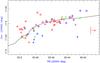 |
Fig. 7 Spatial distribution of Class I (red stars), flat-spectrum-spectrum (green stars), and Class II (blue stars) YSOs. The continuous line running from south-east to north-west marks the highest H2 column density line of the filament along its long axis. |
The spatial distribution of young stars is a useful tool for constructing star formation scenario of molecular cloud complexes (e.g., Kumar et al. 2007; Yun et al. 2008; Povich et al. 2009; De Marchi et al. 2011; Jose et al. 2012; Pandey et al. 2013a,b; Mallick et al. 2013; Gouliermis et al. 2014; Panwar et al. 2014; Massi et al. 2015). To understand the star formation scenario of the IRDC G192.76+00.10 region, we plotted the spatial distribution of its YSO content in Fig. 7. In Fig. 7, the continuous solid line is the highest H2 column density line of the filament along its major axis. To define the column density line, we first created an H2 column density map from the 13CO column density map, and then traced its crests by applying a spatial filtering to its intensity distribution. The H2 column density map was constructed from the 13CO column density map using the relations n(12CO) /n(13CO) = 45 and n(12CO) /n(H2) = 8 × 10⁻⁵ (Chavarría et al. 2008, and references therein). In Fig. 7, one notices that the majority of the YSO candidates are aligned closely with the highest column density line of the filament. This close alignment strongly suggests that the formation of the YSOs seems to be continuing in the dense regions of this filamentary cloud along its long axis.
We find that the mean H2 column density of the highest density line is ~1.1 × 1022 cm-2, which corresponds to a mean AV~ 10 mag (using N(H2) = 0.94 × 10 21AV cm-2 mag-1; Bohlin et al. 1978). This agrees with the value (i.e, AV~ 8 mag) expected for filaments above which they are super-critical and capable of forming stars (André et al. 2010, 2011). The projected distances of the identified YSOs from the highest column density line range from 0.05 to 1.5 pc, with ~70% falling within 0.4 pc. This narrow separation is a strong indication of the fact that the core formation in this filamentary dark cloud is not random. Their formation has occurred mainly along the long axis of the filament. Also these YSOs have probably been formed recently, because they possibly did not have enough time to move away from their birth locations. The typical velocity dispersion seen in relatively evolved clusters and association is roughly a few km s-1 (Madsen et al. 2002). In a recent work, Foster et al. (2015) have shown that the 1−2 Myr old Class II stars of the NGC 1333 star-forming region have an intrinsic velocity dispersion of ~1 km s-1, and the average velocity dispersion of the dense cores of the region is around 0.5 km s-1. Thus, the possibility that a few evolved YSOs might have migrated from their birth locations exists; however, in general, protostars are the coldest objects, so are expected to be embedded within the cores. For example, in the OMC-3 region, Takahashi et al. (2013) observed eight out of sixteen Spitzer sources are associated with the SMA continuum cores (observed with a spatial resolutions ~4.5′′, comparable to MIPS), which are identified as protostars, and six out of sixteen are categorized as T-Tauri stars having no counterparts in the SMA continuum emission. In the IRDC G192+00.10 region, most of the identified YSOs are protostellar in nature. If we assume that these protostars have been moved from their birth locations with a velocity close to 0.5 km s-1, their current locations (≤0.4 pc) from the highest density line indicate that the formation of these protostars might have occurred in the past few ×105 yr.
In young filaments, the distribution of cores is thought to represent a possible preferred length-scale of the filament fragmentation (e.g., Muñoz et al. 2007; Jackson et al. 2010; Hacar & Tafalla 2011; Miettinen & Offner 2013; Takahashi et al. 2013). Since cores are the precursors to protostars, the distribution and separation of young protostars is a good proxy for testing the filament fragmentation theory. To do so, we determined the distribution of the projected separation and projected nearest-neighbor (NN) separation among the YSOs as shown in Fig. 8. Although the projected separation among the YSOs varies in the range 0.1−6.0 pc, the NN separation of the majority of the YSOs shows a very narrow range (i.e., 0.1−0.5 pc) with a median ~0.19 pc. Identification and distribution of cores at longer wavelengths are often limited by the spatial resolution and sensitivity of instruments. So far only a very limited number of millimetre and submillimetre observational studies on filaments have been done that achieve an angular resolution that is comparable to, or better than, the existing IR data (i.e., a few arcsec resolution). For example, with the high angular resolution observations a separation of cores ~0.19 pc (Zhang et al. 2009, beam ~1.2′′), ~0.18 pc (Ragan et al. 2015, beam ~2′′), and ~0.25 pc (Takahashi et al. 2013, beam ~4.5′′) have been observed in the filamentary clouds IRDC G28.34+0.06, G011.11-0.12 and OMC-3, respectively. These results seem to be consistent with the median separation of the YSOs observed in the IRDC G192.76+00.10 region.
Theoretically, it is believed that self-gravitating filaments are unstable to fragmentation and that they lead to star forming cores (e.g., Nagasawa 1987; Tomisaka 1995). Thus, it is tempting to think that the formation of YSOs observed in the IRDC G192.76+00.10 region could be the result of the filament fragmentation. In Sect. 4, we therefore discuss whether the observed distribution and separation of YSOs bear an imprint of fragmentation and core formation of the IRDC G192.76+00.10 filamentary cloud.
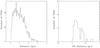 |
Fig. 8 Left: distribution of the projected distances among the sources detected at 24 μm. Right: distribution of the nearest-neighbour separation among the YSOs. |
3.6. Properties of the YSOs
It is very difficult to infer the stellar and circumstellar properties of young protostars based on photometric observations alone. Theoretical models that reproduce the observed SEDs represent the underlying source properties well.
For deep insight into the nature of the detected YSOs, we fitted radiative transfer models of Robitaille et al. (2006, 2007) to their observed SEDs. Interpreting SEDs using the radiative transfer code is subject of degeneracy and spatially resolved multi-wavelength observations can reduce the degeneracy. We thus compiled counterparts of the YSOs at NIR (J, H, and K; this work), IRAC (3.6, 4.5, 5.8, and 8.0 μm; Chavarría et al. 2008), WISE (3.4, 4.6, 12.0, and 22.0 μm; Cutri et al. 2012), MIPS (24 μm and 70 μm; this work), and AKARI (65, 90, 140, and 160 μm; Yamamura et al. 2009) bands, wherever available. We fitted the models to only those sources for which we have flux values at least in five bands in the wavelength range from 1 μm to 24 μm.
While fitting models to the observed fluxes, we adopted the following approaches: i) when IRAC 3.6 μm and 4.5 μm fluxes were available, the WISE fluxes at 3.4 μm and 4.6 μm were not used; ii) for sources not detected at 70 μm or 65 μm, we set the upper limits at these bands by assigning the minimum 70 μm or 65 μm detection flux obtained for the point sources detected in the region. The 70 μm flux upper limit is assigned only to those sources that are not detected in the 70 μm observed area. For sources that are located outside the 70 μm observed area and not detected in 65 μm band, we assigned the minimum 65 μm flux obtained for the point sources observed in the region from the AKARI survey; iii) we scaled the SED models to the distance of the filament (i.e., 2.5 ± 0.2 kpc; Chavarría et al. 2008) and allowed a maximum AV value determined by tracing back the YSOs’ current location on J vs. J − H or K vs. H − K or K vs. K − [ 3.4 ] diagram to the intrinsic dwarf locus along the reddening vector (see, e.g., Samal et al. 2010).
Figure 9 shows the SEDs of 38 sources that satisfy our five data-point flux criteria. The lack of optical, far-infrared, and millimetre data points makes it very apparent that the SED models show high degree of degeneracy; nonetheless, the SEDs clearly indicate that the majority possess IR-excess emission, which is possibly emission from the circumstellar disk and envelope. While looking at Fig. 9, we found that the observed SEDs of four sources (IDs. 4, 18, 19, and 29) in Fig. 9 are fitted well by reddened stellar photosphere models. We find that they correspond to those four sources that have been rejected as YSO candidates in Sect. 3.2 on the basis of their location on the [3.4] vs. [3.4]−[24] diagram (i.e., sources with [3.4]−[24] colour <1 mag). Thus, the SED models confirm our previous results that the bright 3.4 μm sources found in the field-star/MS zone of [3.4] vs. [3.4]−[24] diagram are indeed diskless stars.
It is not possible to characterize all the SED parameters from the models owing to the
limited observational data. However, as discussed in Robitaille et al. (2007), some of the parameters can still be constrained
depending on the available fluxes. For example, in the present study, the SED models
between 1 μm
to 70 μm
represent the data fairly well for the majority of the sources, so the disk parameters are
expected to be better constrained. However, it is worth noting that precise determination
of disk parameters using SED models, as demonstrated by Spezzi et al. (2013), requires data from optical to millimetre bands, as well as
good knowledge of the physical parameters of the central star. Similarly, as discussed in
Robitaille et al. (2006), the disk is expected
to be deeply embedded inside the envelope in the case of young protostars, and the
relative contributions of the disk and envelope to the SED are difficult to disentangle.
For these reasons, in the present case, the uncertainty in the disk parameters is expected
to be high; nonetheless they should give better idea about the nature of the sources. In
Table 2, the disk parameters (disk mass
(Mdisk) and disk accretion rate
(Ṁdisk)) are tabulated. Since our SED
models are highly degenerate, the best-fit model is unlikely to give a unique solution, so
the tabulated values in Table 2 are the weighted
mean and standard deviation of the physical parameters obtained from the models that
satisfy  weighted by
e(−χ2/2) of each
model, where
weighted by
e(−χ2/2) of each
model, where  is the
goodness-of-fit parameter for the best-fit model and Ndata is the
number of input observational data points (see Samal et
al. 2012). In Table 2, we find that the
disk masses and disk accretion rates of ~80% YSOs are in the range 0.001−0.021 M⊙ and
0.01−0.95 × 10⁻⁶M⊙/yr,
respectively. We note that in addition to the limitations outlined above that the absolute
uncertainties associated with the disk parameters are possibly in a range of
1−3 orders of magnitude (see
Robitaille et al. 2007). Therefore, we stress
that the derived disk parameters must be considered as representative values, so should be
treated with caution.
is the
goodness-of-fit parameter for the best-fit model and Ndata is the
number of input observational data points (see Samal et
al. 2012). In Table 2, we find that the
disk masses and disk accretion rates of ~80% YSOs are in the range 0.001−0.021 M⊙ and
0.01−0.95 × 10⁻⁶M⊙/yr,
respectively. We note that in addition to the limitations outlined above that the absolute
uncertainties associated with the disk parameters are possibly in a range of
1−3 orders of magnitude (see
Robitaille et al. 2007). Therefore, we stress
that the derived disk parameters must be considered as representative values, so should be
treated with caution.
Owing to several limitations, it is not possible to comment on individual objects, but if we take the SED results for statistical purposes, the derived disk accretion rates suggest that the YSOs of the IRDC G192.76+00.10 region are mainly low-mass in nature (e.g., Dahm 2008), which is consistent with the nature of the sources derived from the photometric data.
Inferred physical parameters from SED fits to YSOs.
 |
Fig. 9 SEDs of the YSOs discussed in the text. The black line shows the best fit model,
and the grey lines show subsequent models that satisfy
|
4. Discussions and conclusions
4.1. Evolutionary status
The protostar fraction (i.e., number of protostars (Class I + Flat-spectrum) of the total number YSO population) in young clusters is a good tracer of age. For example, the protostar fraction derived from the data involving 2.2−24 μm is 14% in the IC 348 cluster of age ~2−3 Myr, ~16% in Chamaeleon II (Alcalá et al. 2008) of age ~2−3 Myr (Sciortino 2007; Spezzi et al. 2008), and ~36% in the NGC 1333 cluster of age ~1−2 Myr (Jørgensen et al. 2006). This suggests an evolutionary difference, with the young NGC 1333 consists of a younger population of YSOs compared to IC 348 and Chamaeleon II. In the IRDC G192.76+00.10 region, we identified a total of 62 YSOs, with 19 are Class II YSOs and 43 that are Class I plus flat-spectrum YSOs. This indicates that this dark cloud is unusually rich in protostars (~70%). This large number strongly suggests that the IRDC G192.76+00.10 region is too young for most YSOs to have reached the Class II stage. In young clusters, the error in the Class ratio in general is dominated by the detection of the actual number of Class I, flat-spectrum and Class II objects. If we consider all the YSOs that are above our completeness limit, we find that the protostar percentage is still high (i.e., ~55%), indicating that the region indeed contains a high percentage of protostars. A comparison of the protostar fraction of the IRDC G192.76+00.10 region with the IC 348, NGC 1333, and Chamaeleon II suggests that the IRDC G192.76+00.10 is indeed young, possibly younger than 1 Myr.
Another possible way to assign age to a star-forming region is to use the lifetime of different phase of YSOs associated in the region. Evans et al. (2009) derived the lifetimes of different YSO phases from a large sample of YSOs collected from five nearby molecular clouds, assuming that in these clouds star formation has proceeded at a constant rate over a 2 Myr period of time and that all the prestellar cores have evolved into Class 0/I YSOs, then into flat-spectrum YSOs, and finally to Class II YSOs. Although the derived lifetimes are still subject to large uncertainties (see Evans et al. 2009, and discussion therein), the above work involving a large set of YSOs suggests that in general a lifetime of Class II, Class I, and flat-spectrum stages of a YSO is roughly ~2, ~0.44, and ~0.35 Myr, respectively. In the IRDC G192.76+00.10 region, we found that most of the identified YSOs are Class I, flat-spectrum, and Class II in nature. If we use the above lifetimes, then the YSOs class statistics suggest a mean age of ~1 Myr for IRDC G192.76+0.10.
4.2. Possible fragmentation process of the IRDC region
The S254-S258 complex harbors a 20 pc long filament. Numerical simulations suggest that there are various processes by which filaments can be formed. Simulation shows that the fragmentation of clouds into sheets and filaments are the natural consequence of the supersonic turbulence present in the inter-stellar medium (Klessen & Burkert 2000; Padoan et al. 2001; Ostriker et al. 2001; Bate 2009). The driving sources for large-scale turbulence could be flows of atomic gas (e.g., Hennebelle et al. 2008; Banerjee et al. 2009), waves from supernova explosions and superbubbles (e.g., Matzner 2002; Dale & Bonnell 2011), or collisions between molecular clouds (e.g., Tasker & Tan 2009). Once filamentary structures formed, theoretical models suggest that they are subject to fragmentation (e.g., Larson 1985).
For an infinite and isothermal filament, the filament is unstable to axisymmetric perturbation, if its line mass Mline (i.e., mass per unit length) value exceeds its critical equilibrium mass value Mcrit =  (e.g., Ostriker 1964), where cs is the sound speed of the medium and G the gravitational constant. The critical line mass only depends on the gas temperature. The temperature of the IRDC G192.76+00.10 cloud is ~14 K (discussed below), which corresponds to Mcrit ~ 25M⊙ pc-1.
The projected size of the IRDC G192.76+00.10 cloud along its long axis is about 5.7 pc. To estimate Mline, we first estimated the radial profile of the filament from the H2 column density map. To do so, we extracted perpendicular column density profiles at several positions along the filamentary structures, and established the radial extent of each profile using Gaussian fitting similar to other works (e.g., Arzoumanian et al. 2011; Smith et al. 2014). We then estimated Mline by dividing the length of the filament to the mass estimated over the mean radial extent of the entire filament, which turns out to be ~120 M⊙ pc-1. The observed line mass is about five times higher than the critical line mass, indicating that the filament is supercritical, hence susceptible to fragmentation. Supercritical filaments are believed to be generally unstable to radial gravitational collapse and fragment into prestellar clumps or cores along their major axis. This is supported by the roughly linear sequence of protostars observed along the long axis of the IRDC G192.76+00.10 region. Recent Herschel observations have also shown that supercritical filaments usually harbour several prestellar cores and Class 0/Class I protostars along their length (e.g., André et al. 2010).
Numerical simulation also suggests that gravitational fragmentation is possibly the dominant mechanism in the formation of cores and stars in the dense regions of the filaments (e.g., Klessen et al. 2004). To further validate the above hypothesis, we compare our results with the simple model of gravitational fragmentation, given by Hartmann (2002). In his model, the fragmentation length (λc) of a cylinder due to gravitational instability is given by  (1)where AV is the visual extinction corresponding to the surface density (Σ) through the centre of the filament and T10 is the gas temperature in units of 10 K. The corresponding collapse timescale is given by
 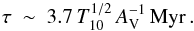 (2)Herschel estimates of dust temperatures indicate that the temperature of the quiescent and star-forming filaments are in the range of 10 K to 15 K (Arzoumanian et al. 2011). Observations of the ammonia (1, 1) and (2, 2) inversion transitions suggest that the kinetic temperature in the dense part of the IRDC G192.76+00.10 filament is in the range of 13 to 15 K (Dunham et al. 2010). Considering 14 K as the temperature of the filament and 10 mag as the mean visual extinction, the above equation predicts λc ~ 0.21 pc and τ ~ 0.45 Myr. For randomly oriented filament, the line-of-sight median inclination angle could be ~60° (Genzel & Stutzki 1989). If this is the case, then this would decrease λc to a value 0.19 pc. Most of the YSOs in the filament are protostars. The lifetime of embedded protostars is around 0.5 Myr. The predicted fragmentation length and collapse time for the region are comparable to the observed median NN separation (~0.2 pc) and age of majority of the YSOs, so the model predictions broadly agree with the observations.
Limitations
The scenario presented above is roughly consistent with the results discussed in Ballesteros-Paredes (2004) and with the scenario preferred for the YSO formation in the Taurus (Hartmann 2002). However, there are several issues still to be addressed. For example, the exact role of turbulence prior to fragmentation is not known to us; its presence would increase the effective sound speed, thereby increasing the critical mass per unit length. However, it is suggested that a prestellar cloud is most likely stabilized against global collapse by interstellar turbulence, but this support quickly disappears on small spatial scales (e.g., Elmegreen et al. 2000).
Recent observations have suggested that the core formation in filamentary clouds is possibly a two-step process, in which the subsonic, velocity-coherent filaments condense out of the more turbulent ambient cloud first. Then, the cores fragment quasi-statically, where turbulence seems to play a little or no role in the formation of the individual cores (e.g., Ballesteros-Paredes 2004; André et al. 2011; Hacar & Tafalla 2011). Based on ammonia observations, Dunham et al. (2010) observed non-thermal velocity dispersion of ~0.43 km s-1 in the central region of IRDC G192.76+00.10. However, non-thermal dispersion in clouds could have various origins. For example, non-thermal motions can be driven by the accretion flows to the filament potential (e.g., Klessen & Hennebelle 2010), if the IRDC G192.76+00.10 filament has undergone dynamical evolution after fragmenaion.
Similarly, protostellar feedback can also drive supersonic turbulence on sub-parsec size scales (e.g., Duarte-Cabral et al. 2012). If the non-thermal motion (corresponding to the velocity dispersion) is to be considered in addition to the thermal component to support the filament, this would then increase the effective sound speed of the filament (e.g., see MacLaren et al. 1988). As a consequence of this, the Mcrit of the filament would increase to ~75 M⊙ pc-1, which is still lower than the observed Mline, implying that the total amount of support available is still insufficient for keeping the filament in equilibrium, so the filament should be radially contracting.
Other physical processes that might affect the model parameters discussed above are the helical magnetic field (Fiege & Pudritz 2000) and star formation from dynamical effects such as flows from surrounding sub-filaments (e.g., Smith et al. 2014; Schneider et al. 2010). Helical magnetic fields are believed to decrease the critical length of fragmentation of a cylinder (Fiege & Pudritz 2000), whose effect is difficult to assess in the present case. However, in case of star formation due to converging flows, a higher concentration of dense gas is expected at the junction point of the converging sub-filaments and the main filament, which tend to increase star formation activity. For example, in the DR21 region, several low-density striations or sub-filaments were observed perpendicular to the main filament, and they were apparently feeding matter to the main filament (e.g., Kumar et al. 2007; Schneider et al. 2010; Hennemann et al. 2012). Considering that the IRDC G192.76+00.10 region is slightly structured on its eastern side, the possibility that few stars might have formed by other dynamical processes cannot be ignored. However, the morphology of the IRDC G192.76+00.10 area is largely linear in CO, and we do not see the strong morphological signature of such structures (e.g., thin long sub-filaments) that are radially attached to the IRDC G192.76+00.10 region, though this cannot be warranted without high resolution and sensitive observations. Nonetheless, to limit the impact of dynamical processes on our estimations, we calculated the model parameters again, without accounting for the group of stars seen around α2000 = 93.50 & δ2000 = + 17.87 (i.e., the group of stars seen distinctly away from the filament’s long axis), as well as a few stars located far away from the highest density line (see Fig. 7). Considering tentatively that these are stars that might have formed by some other processes, we found that the model parameters are only changed by 20%.
We also stress that even though smooth cylindrical models are useful for understanding star formation processes in filaments, they can only represent a first-order approximation because real clouds are likely to have much more inhomogeneities in density than what we have assumed here. In addition to this, the initial cloud configuration also plays a decisive role where stars would form. For example, if the original parental cloud is not infinitely long or spherical, gravitational-edge focusing results in enhanced concentrations of mass at one end of the filament, where local collapse would proceed faster than collapse of the entire filament (e.g., Burkert & Hartmann 2004). We do not observe high concentration of stars or massive condensations at any end of the IRDC G192.76+00.10 region, thus the gravitational edge focusing effect is preferably not happening here.
In summary, the caveats outlined above prevent us from making any definite statement about the YSO formation; however, if we consider the roles of the helical magnetic field and star formation by other dynamical processes are minimum, then we find a remarkable reconciliation of the observed properties with the model predictions, suggesting that gravitational fragmentation is probably the dominant cause of core formation in the IRDC G192.76+00.10 filamentary cloud. Confirming and refining the scenario require high angular resolution mid-infrared, dust polarimetric, and millimetre line observations to identify other possible low-mass YSOs, to constrain the roles of the magnetic field and the influence of gravity, in the star formation processes of the region.
4.3. Star formation efficiency and rate
In this section, we discuss the star formation efficiency (SFE) and star formation rate (SFR) of the IRDC G192.76+00.10 region based on the YSOs identified in the present work. SFE and SFR are the fundamental physical parameters that are essential for understanding the evolution of star-forming regions and galaxies.
The SFE is defined as the ratio of the total stellar mass to the total mass of stars and gas. We estimate the total gaseous mass (Mgas) associated to the IRDC region ~1100 M⊙, using the 13CO column density map and integrated the column density four times above the local background, i.e., column density value > 1.1 × 1016 cm-2 over 11 pc2 area. We then converted the total 13CO column density to the total H2 column density as discussed in Sect. 3.5, and used the following equation to estimate the mass: 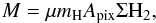 (3)where μ is the mean molecular weight, mH the mass of the hydrogen atom, Σ H2 is the summed H2 column density, and Apix the area of a pixel in cm-2 at the distance of the region. The determination of the stellar mass in accreting stars is not trivial, because emission due to circumstellar disk surrounding the star and accreting material from the protoplanetary disk onto the central star affects the observed spectrum. Broad-band spectroscopic observation would reveal more accurate mass of the YSOs (e.g., Manara et al. 2013); however, if we assume that each source of the IRDC G192.76+00.10 region has a mass of 0.5 M⊙ (close to the mean stellar mass of the region; see Sect. 3.4), consistent with the characteristic mass from the studies of the Chabrier (2003) and Kroupa (2001) type of the initial mass function (IMF), then the total mass of all the YSOs (MYSOs) turned out to be ~30 M⊙. Using the Mgas and MYSOs, we estimated the SFE ~0.03 or 3% in the IRDC G192.76+00.10 region.
The SFR describes the rate at which the gas in a cloud is turning into stars. Assuming 1 Myr as the duration of star formation (see Sect. 4.1) and using the derived Mgas and MYSOs, we estimated the SFR (=Mgas × SFE /tsf, where tsf is the star formation time scale) of the IRDC G192.76+00.10 region ~30 M⊙ Myr-1. The projected area of the IRDC G192.76+00.10 region over which we estimated the cloud mass is ~11 pc2. If we normalized the derived SFR by the cloud area, this leads to a SFR per unit surface area ~3 M⊙ Myr-1 pc-2. The SFE and SFR per unit surface area of the IRDC G192.76+00.10 region are comparable to the SFE (i.e., 3−6%) and SFR per unit surface area (i.e., 0.6−3.2 M⊙ Myr-1 pc-2) values reported by Evans et al. (2009) for nearby molecular cloud complexes.
Since our YSOs sample is complete down to ~0.15 M⊙, we may thus be missing a population of deeply embedded YSOs of masses below this completeness level. If we assume that the cloud has already formed stars down to the hydrogen-burning limit (i.e., ~0.08 M⊙), this would not drastically alter the SFE of the complex, because most of the observations in our Galaxy are consistent with an IMF that declines below 0.1 M⊙ (e.g., Lada 2005; Andersen et al. 2008; Oliveira et al. 2009; Neichel et al. 2015). Thus, we do not expect a large population of Class II and Class I YSOs below our completeness limit. The shape and universality of the IMF in the sub-stellar regime is still being debated, however, assuming Chabrier (2003) type of mass function, we may probably be missing only about 20% of the total number of YSOs. This may increase the SFE of the region by only about 1%, assuming each YSO has a mass 0.5 M⊙.
4.4. Emerging young cluster
Detection and identification of clumps and cores in star-forming complexes using long wavelength observations depend on the resolution and sensitivity of surveys. For example, the dust clump “P1” of the G28.34+0.06 region detected with the IRAM 30 m telescope and JCMT at resolutions from 11′′ to 15′′ (Rathborne et al. 2006; Carey et al. 1998) are resolved by the Submillimeter Array (SMA) into five cores at 1.̋2 resolution (Zhang et al. 2009). So far, no high-resolution observations have been conducted to identify clumps and cores of the IRDC G192.76+00.10 region. In this work, we have detected protostellar sources of mass down to 0.15 M⊙, so millimetre continuum observations of mass sensitivities higher than 0.45 M⊙ (assuming the SFE of cores is ~30%; Alves et al. 2007) and spatial resolution higher than Spitzer observations would be very helpful for detecting of resolved cores in the region. Nonetheless, using the 1.1 millimetre Bolocam Galactic Plane Survey (BGPS; beam ~33′′), Dunham et al. (2010) observed an elongated clump (their ID 50) in the central area of IRDC G192.76+00.10. From their observation, we estimated the virial parameter (Bertoldi & McKee 1992) of the clump ~0.3. The virial parameter represents the dynamical stability of a core or clump. A clump is assumed to be gravitationally bound if its virial parameter value is ≤1 and unbound otherwise. The virial parameter value of the BGPS clump suggests that the clump is susceptible to gravitational collapse, so can lead to star formation.
The filament in which the BGPS clump is embedded is in super-critical (discussed in Sect. 4.2.1) stage, implying that the filamentary cloud may be contracting. Moreover, observations and simulations of filaments show accretion flows along the filaments onto the clumps and cores located at the bottom of their potential (Balsara et al. 2001; Kirk et al. 2013; Tackenberg et al. 2014), and some clumps and cores possibly accrete mass faster than others owing to their higher gravitational potential (e.g., Tackenberg et al. 2014). Observations suggest that star-forming clouds dynamically evolve on time scales of a few Myr. If it is to be believed that cluster formation mainly occurs in filamentary clouds, then the lifetime of the typical filament should be a few Myr, since clusters with ages over 5 Myr are found to seldom be associated with molecular gas (e.g., Leisawitz et al. 1989). In Sect. 4.1, we have estimated that the age of the IRDC G192.76+00.10 region is around 1 Myr. If we put all our results in context, they suggest that the YSOs of the IRDC G192.76+00.10 region are young. They are embedded in a gas reservoir of mass ~1100 M⊙, the dark cloud is forming stars at a high rate of ~30 M⊙ Myr-1, and it is part of a large filament environment where individual clumps and cores can grow in mass by accreting matter from the parental filament to their potentials. This evidence suggests that if the dark cloud evolves dynamically for a few Myr, then the possibility that it may emerge into a richer cluster exists.
4.5. Overall picture of star formation in the complex
The 20 pc long filament of the S254-S258 complex consists of six evolved H ii regions. Among these, four H ii regions (S254, S255, S256, and S257) are located at the centre of the complex at a mean separation of 2.6 pc (see Fig. 1). The exciting stars of S254, S255 and S257 are isolated sources, without any co-spatial clustering of low-mass stars around them. The mean dynamical age of these evolved H ii regions is ~2.5 Myr (see Chavarría et al. 2008). It seems that the evolved massive stars (exciting stars of evolved H ii regions) in this complex must have formed about 2.5 Myr ago.
In this work, we characterized the protostellar population of the IRDC G192.76+00.10 region, which is located farther away from the evolved H ii regions of the complex. Although the low-mass YSOs in the IRDC G192.76+00.10 region are at different evolutionary stages, the majority (~70%) of them are Class I and flat-spectrum in nature. The typical lifetime of Class I and flat-spectrum objects is around 0.4 Myr (Evans et al. 2009). Therefore, it is very likely that the majority of the YSOs in the IRDC G192.76+00.10 region were formed simultaneously or over a narrow range of time, possibly less than 0.5 Myr of time.
The evolutionary status of the high-mass OB stars (age ~2.5 Myr) and low-mass protostars of the IRDC G192.76+00.10 region (age ~0.5 Myr) suggests there is multi-generation star formation in the complex. The evolved H ii regions (e.g., S255, and S257) appear to be projected on the long filament. If all the optically visible evolved H ii regions and the low-mass protostars of the IRDC G192.76+00.10 region are part of the same long (~20 pc) filament, it is then plausible to think that multiple generations of stars may be residing in the whole filament. If this is the case, then the whole filament probably has not fragmented as a single entity.
Hierarchical fragmentation has also been observed in several filamentary clouds (e.g., Hacar & Tafalla 2011; Takahashi et al. 2013). For example, in the Orion filamentary cloud, Takahashi et al. (2013) find different fragmentation scales for large-scale clumps (9−10 pc), small-scale clumps (~2.5 pc), and dense cores (0.15−0.55 pc), and interpret this result as the hierarchical fragmentation of the Orion A filament. Thus, the possibility that the long filament of the S254-S258 complex has undergone hierarchical fragmentation cannot be ruled out. Hierarchical fragmentation in clouds could have various origins. For example, it could be due to combined effect of turbulence, cloud temperature, magnetic field, and ionization from the massive stars as discussed in Takahashi et al. (2013) or as discussed in Vázquez-Semadeni et al. (2009), where low-mass and high-mass star-forming regions can arise from the hierarchical gravitational collapse of a large cloud, where the former regions arise from collapse of small-scale fragments, and where the latter may appear due to large-scale collapse.
4.6. Concluding remarks
In this paper, we have presented a dark cloud (mainly consists of low-mass stars) based on MIPS, WISE and JHK photometry. It harbours 62 YSOs, 49 of which contain 24 μm sources, indicating that the cluster is young. Interestingly, the dark cloud is found in the filament of an OB complex, with members distributed in an aligned fashion along the long axis of the filament and at an NN separation ~0.2 pc. We found that the protostars to Class II ratio in the dark cloud is high (~2). When compared to other star-forming regions, it indicates that the region is young, possibly younger than 1 Myr. From our results, we also find evidence that gravitational fragmentation is the dominant cause of YSOs formation in this dark cloud, but a conclusive answer would require a further large-scale study of the filament concerning magnetic field, turbulence, and gravity. The lack of deep infrared observations prevents us from making a definite conclusion about the properties of the cloud; however, from the present observations, we argued that the cloud is currently forming a cluster at an efficiency of ~3% and a rate of ~30 M⊙ Myr-1. The cluster is embedded in a supercritical filamentary dark cloud of mass ~1100 M⊙ and is part of a large filament geometry. We hypothesized that it may become a richer cluster with time. Because of the lack of massive protostars, the possibility of radiative heating and photo-evaporation of the dense gas in the studied filament region is low, so that the dark cloud provides a unique opportunity with high sensitive observations to gain a deeper understanding of cluster formation and evolution within the filamentary environment.
Acknowledgments
We thank the anonymous referee for a critical reading of the paper and several useful constructive comments and suggestions, that improved the scientific content of the paper. We thank Dr. L. Chavarría for allowing us to use their CO column density map. M.R.S. thanks the Tata Institute of Fundamental Research (TIFR) for the kind hospitality during his visits to the institute, where a part of this work was carried out. M.R.S. also acknowledges the financial support provided by the French Space Agency (CNES) for his postdoctoral fellowship. D.K.O. and I.Z. acknowledge support from DST-RFBR project (P-142; 13-02-92627). The I.Z. research was partly supported by the grant within the agreement No. 02.49.21.0003 between the Ministry of education and science of the Russian Federation and Lobachevsky State University of Nizhni Novgorod.
References
- Alcalá, J. M., Spezzi, L., Chapman, N., et al. 2008, ApJ, 676, 427 [NASA ADS] [CrossRef] [Google Scholar]
- Alves, J., Lombardi, M., & Lada, C. J. 2007, A&A, 462, L17 [NASA ADS] [CrossRef] [EDP Sciences] [Google Scholar]
- Andersen, M., Meyer, M. R., Greissl, J., & Aversa, A. 2008, ApJ, 683, L183 [NASA ADS] [CrossRef] [Google Scholar]
- André, P. 2013, ArXiv e-prints [arXiv:1309.7762] [Google Scholar]
- André, P., Ward-Thompson, D., & Barsony, M. 2000, Protostars and Planets IV, 59 [Google Scholar]
- André, P., Men’shchikov, A., Bontemps, S., et al. 2010, A&A, 518, L102 [NASA ADS] [CrossRef] [EDP Sciences] [Google Scholar]
- André, P., Men’shchikov, A., Könyves, V., & Arzoumanian, D. 2011, in Computational Star Formation, eds. J. Alves, B. G. Elmegreen, J. M. Girart, & V. Trimble, IAU Symp., 270, 255 [Google Scholar]
- Arzoumanian, D., André, P., Didelon, P., et al. 2011, A&A, 529, L6 [Google Scholar]
- Ballesteros-Paredes, J. 2004, Ap&SS, 292, 193 [NASA ADS] [CrossRef] [Google Scholar]
- Balsara, D., Ward-Thompson, D., & Crutcher, R. M. 2001, MNRAS, 327, 715 [NASA ADS] [CrossRef] [Google Scholar]
- Banerjee, R., Vázquez-Semadeni, E., Hennebelle, P., & Klessen, R. S. 2009, MNRAS, 398, 1082 [NASA ADS] [CrossRef] [Google Scholar]
- Baraffe, I., Chabrier, G., Barman, T. S., Allard, F., & Hauschildt, P. H. 2003, A&A, 402, 701 [NASA ADS] [CrossRef] [EDP Sciences] [Google Scholar]
- Bate, M. R. 2009, MNRAS, 397, 232 [NASA ADS] [CrossRef] [Google Scholar]
- Battersby, C., Bally, J., Ginsburg, A., et al. 2011, A&A, 535, A128 [NASA ADS] [CrossRef] [EDP Sciences] [Google Scholar]
- Bertoldi, F., & McKee, C. F. 1992, ApJ, 395, 140 [NASA ADS] [CrossRef] [Google Scholar]
- Beuther, H., & Sridharan, T. K. 2007, ApJ, 668, 348 [NASA ADS] [CrossRef] [Google Scholar]
- Bieging, J. H., Peters, W. L., Vi la Vilaro, B., Schlottman, K., & Kulesa, C. 2009, AJ, 138, 975 [NASA ADS] [CrossRef] [Google Scholar]
- Bohlin, R. C., Savage, B. D., & Drake, J. F. 1978, ApJ, 224, 132 [NASA ADS] [CrossRef] [Google Scholar]
- Brand, J., Massi, F., Zavagno, A., Deharveng, L., & Lefloch, B. 2011, A&A, 527, A62 [NASA ADS] [CrossRef] [EDP Sciences] [Google Scholar]
- Burkert, A., & Hartmann, L. 2004, ApJ, 616, 288 [NASA ADS] [CrossRef] [Google Scholar]
- Carey, S. J., Clark, F. O., Egan, M. P., et al. 1998, ApJ, 508, 721 [NASA ADS] [CrossRef] [Google Scholar]
- Carey, S. J., Noriega-Crespo, A., Mizuno, D. R., et al. 2009, PASP, 121, 76 [NASA ADS] [CrossRef] [Google Scholar]
- Carpenter, J. M., Snell, R. L., & Schloerb, F. P. 1995, ApJ, 450, 201 [NASA ADS] [CrossRef] [Google Scholar]
- Casali, M., Adamson, A., Alves de Oliveira, C., et al. 2007, A&A, 467, 777 [NASA ADS] [CrossRef] [EDP Sciences] [Google Scholar]
- Chabrier, G. 2003, PASP, 115, 763 [NASA ADS] [CrossRef] [Google Scholar]
- Chavarría, L. A., Allen, L. E., Hora, J. L., Brunt, C. M., & Fazio, G. G. 2008, ApJ, 682, 445 [NASA ADS] [CrossRef] [Google Scholar]
- Chen, W. P., Pandey, A. K., Sharma, S., et al. 2011, AJ, 142, 71 [NASA ADS] [CrossRef] [Google Scholar]
- Chu, Y.-H., & Gruendl, R. A. 2008, in Massive Star Formation: Observations Confront Theory, eds. H. Beuther, H. Linz, & T. Henning, ASP Conf. Ser., 387, 415 [Google Scholar]
- Condon, J. J., Cotton, W. D., Greisen, E. W., et al. 1998, AJ, 115, 1693 [NASA ADS] [CrossRef] [Google Scholar]
- Connelley, M. S., & Greene, T. P. 2010, AJ, 140, 1214 [NASA ADS] [CrossRef] [Google Scholar]
- Crapsi, A., van Dishoeck, E. F., Hogerheijde, M. R., Pontoppidan, K. M., & Dullemond, C. P. 2008a, A&A, 486, 245 [NASA ADS] [CrossRef] [EDP Sciences] [Google Scholar]
- Crapsi, A., van Dishoeck, E. F., Hogerheijde, M. R., Pontoppidan, K. M., & Dullemond, C. P. 2008b, A&A, 486, 245 [NASA ADS] [CrossRef] [EDP Sciences] [Google Scholar]
- Cutri, R. M., Skrutskie, M. F., van Dyk, S., et al. 2003, VizieR Online Data Catalog: II/246 [Google Scholar]
- Cutri, R. M., et al. 2012, VizieR Online Data Catalog: II/31 [Google Scholar]
- Dahm, S. E. 2008, AJ, 136, 521 [NASA ADS] [CrossRef] [Google Scholar]
- Dale, J. E., & Bonnell, I. 2011, MNRAS, 414, 321 [NASA ADS] [CrossRef] [Google Scholar]
- De Marchi, G., Panagia, N., & Sabbi, E. 2011, ApJ, 740, 10 [NASA ADS] [CrossRef] [Google Scholar]
- Deharveng, L., Schuller, F., Anderson, L. D., et al. 2010, A&A, 523, A6 [NASA ADS] [CrossRef] [EDP Sciences] [Google Scholar]
- Deharveng, L., Zavagno, A., Anderson, L. D., et al. 2012, A&A, 546, A74 [NASA ADS] [CrossRef] [EDP Sciences] [Google Scholar]
- Duarte-Cabral, A., Chrysostomou, A., Peretto, N., et al. 2012, A&A, 543, A140 [NASA ADS] [CrossRef] [EDP Sciences] [Google Scholar]
- Dunham, M. K., Rosolowsky, E., Evans, II, N. J., et al. 2010, ApJ, 717, 1157 [NASA ADS] [CrossRef] [Google Scholar]
- Elmegreen, B. G., & Lada, C. J. 1977, ApJ, 214, 725 [NASA ADS] [CrossRef] [Google Scholar]
- Elmegreen, B. G., Efremov, Y., Pudritz, R. E., & Zinnecker, H. 2000, Protostars and Planets IV, 179 [Google Scholar]
- Engelbracht, C. W., Blaylock, M., Su, K. Y. L., et al. 2007, PASP, 119, 994 [NASA ADS] [CrossRef] [Google Scholar]
- Evans, II, N. J., Allen, L. E., Blake, G. A., et al. 2003, PASP, 115, 965 [NASA ADS] [CrossRef] [Google Scholar]
- Evans, II, N. J., Dunham, M. M., Jørgensen, J. K., et al. 2009, ApJS, 181, 321 [NASA ADS] [CrossRef] [Google Scholar]
- Fiege, J. D., & Pudritz, R. E. 2000, MNRAS, 311, 105 [NASA ADS] [CrossRef] [Google Scholar]
- Flaherty, K. M., Pipher, J. L., Megeath, S. T., et al. 2007, ApJ, 663, 1069 [CrossRef] [Google Scholar]
- Foster, J. B., Cottaar, M., Covey, K. R., et al. 2015, ApJ, 799, 136 [NASA ADS] [CrossRef] [Google Scholar]
- Genzel, R., & Stutzki, J. 1989, ARA&A, 27, 41 [NASA ADS] [CrossRef] [Google Scholar]
- Getman, K. V., Feigelson, E. D., Sicilia-Aguilar, A., et al. 2012, MNRAS, 426, 2917 [NASA ADS] [CrossRef] [Google Scholar]
- Gouliermis, D. A., Hony, S., & Klessen, R. S. 2014, MNRAS, 439, 3775 [NASA ADS] [CrossRef] [Google Scholar]
- Guieu, S., Rebull, L. M., Stauffer, J. R., et al. 2010, ApJ, 720, 46 [NASA ADS] [CrossRef] [Google Scholar]
- Hacar, A., & Tafalla, M. 2011, A&A, 533, A34 [NASA ADS] [CrossRef] [EDP Sciences] [Google Scholar]
- Hambly, N. C., Collins, R. S., Cross, N. J. G., et al. 2008, MNRAS, 384, 637 [NASA ADS] [CrossRef] [Google Scholar]
- Hartmann, L. 2002, ApJ, 578, 914 [NASA ADS] [CrossRef] [Google Scholar]
- Heitsch, F., Ballesteros-Paredes, J., & Hartmann, L. 2009, ApJ, 704, 1735 [NASA ADS] [CrossRef] [Google Scholar]
- Hennebelle, P., Banerjee, R., Vázquez-Semadeni, E., Klessen, R. S., & Audit, E. 2008, A&A, 486, L43 [NASA ADS] [CrossRef] [EDP Sciences] [Google Scholar]
- Hennemann, M., Motte, F., Schneider, N., et al. 2012, A&A, 543, L3 [NASA ADS] [CrossRef] [EDP Sciences] [Google Scholar]
- Henning, T., Linz, H., Krause, O., et al. 2010, A&A, 518, L95 [NASA ADS] [CrossRef] [EDP Sciences] [Google Scholar]
- Indebetouw, R., Robitaille, T. P., Whitney, B. A., et al. 2007, ApJ, 666, 321 [NASA ADS] [CrossRef] [Google Scholar]
- Jackson, J. M., Finn, S. C., Chambers, E. T., Rathborne, J. M., & Simon, R. 2010, ApJ, 719, L185 [NASA ADS] [CrossRef] [Google Scholar]
- Jørgensen, J. K., Harvey, P. M., Evans, II, N. J., et al. 2006, ApJ, 645, 1246 [NASA ADS] [CrossRef] [Google Scholar]
- Jose, J., Pandey, A. K., Ogura, K., et al. 2012, MNRAS, 424, 2486 [NASA ADS] [CrossRef] [Google Scholar]
- Jose, J., Pandey, A. K., Samal, M. R., et al. 2013, MNRAS, 432, 3445 [NASA ADS] [CrossRef] [Google Scholar]
- Kirk, H., Myers, P. C., Bourke, T. L., et al. 2013, ApJ, 766, 115 [NASA ADS] [CrossRef] [Google Scholar]
- Klessen, R. S., & Burkert, A. 2000, ApJS, 128, 287 [NASA ADS] [CrossRef] [Google Scholar]
- Klessen, R. S., & Hennebelle, P. 2010, A&A, 520, A17 [NASA ADS] [CrossRef] [EDP Sciences] [Google Scholar]
- Klessen, R. S., Ballesteros-Paredes, J., Li, Y., & Mac Low, M.-M. 2004, in The Formation and Evolution of Massive Young Star Clusters, eds. H. J. G. L. M. Lamers, L. J. Smith, & A. Nota, ASP Conf. Ser., 322, 299 [Google Scholar]
- Koenig, X. P., Leisawitz, D. T., Benford, D. J., et al. 2012, ApJ, 744, 130 [NASA ADS] [CrossRef] [Google Scholar]
- Kroupa, P. 2001, MNRAS, 322, 231 [NASA ADS] [CrossRef] [Google Scholar]
- Kumar, M. S. N., Davis, C. J., Grave, J. M. C., Ferreira, B., & Froebrich, D. 2007, MNRAS, 374, 54 [NASA ADS] [CrossRef] [Google Scholar]
- Lada, C. J. 1987, in Star Forming Regions, eds. M. Peimbert, & J. Jugaku, IAU Symp., 115, 1 [Google Scholar]
- Lada, C. J. 2005, in The Initial Mass Function 50 Years Later, eds. E. Corbelli, F. Palla, & H. Zinnecker, Astrophys. Space Sci. Library, 327, 109 [Google Scholar]
- Larson, R. B. 1985, MNRAS, 214, 379 [NASA ADS] [Google Scholar]
- Leisawitz, D., Bash, F. N., & Thaddeus, P. 1989, ApJS, 70, 731 [NASA ADS] [CrossRef] [Google Scholar]
- Longmore, S. N., Rathborne, J., Bastian, N., et al. 2012, ApJ, 746, 117 [NASA ADS] [CrossRef] [Google Scholar]
- MacLaren, I., Richardson, K. M., & Wolfendale, A. W. 1988, ApJ, 333, 821 [NASA ADS] [CrossRef] [Google Scholar]
- Madsen, S., Dravins, D., & Lindegren, L. 2002, A&A, 381, 446 [NASA ADS] [CrossRef] [EDP Sciences] [Google Scholar]
- Mallick, K. K., Kumar, M. S. N., Ojha, D. K., et al. 2013, ApJ, 779, 113 [NASA ADS] [CrossRef] [Google Scholar]
- Manara, C. F., Beccari, G., Da Rio, N., et al. 2013, A&A, 558, A114 [NASA ADS] [CrossRef] [EDP Sciences] [Google Scholar]
- Massi, F., Giannetti, A., Di Carlo, E., et al. 2015, A&A, 573, A95 [NASA ADS] [CrossRef] [EDP Sciences] [Google Scholar]
- Matzner, C. D. 2002, ApJ, 566, 302 [NASA ADS] [CrossRef] [Google Scholar]
- Meyer, M. R., Calvet, N., & Hillenbrand, L. A. 1997, AJ, 114, 288 [NASA ADS] [CrossRef] [Google Scholar]
- Miettinen, O., & Offner, S. S. R. 2013, A&A, 555, A41 [NASA ADS] [CrossRef] [EDP Sciences] [Google Scholar]
- Molinari, S., Swinyard, B., Bally, J., et al. 2010, A&A, 518, L100 [NASA ADS] [CrossRef] [EDP Sciences] [Google Scholar]
- Muñoz, D. J., Mardones, D., Garay, G., et al. 2007, ApJ, 668, 906 [NASA ADS] [CrossRef] [Google Scholar]
- Mucciarelli, P., Preibisch, T., & Zinnecker, H. 2011, A&A, 533, A121 [NASA ADS] [CrossRef] [EDP Sciences] [Google Scholar]
- Myers, P. C. 2009, ApJ, 700, 1609 [NASA ADS] [CrossRef] [EDP Sciences] [Google Scholar]
- Myers, P. C., Adams, F. C., Chen, H., & Schaff, E. 1998, ApJ, 492, 703 [NASA ADS] [CrossRef] [Google Scholar]
- Nagasawa, M. 1987, Prog. Theor. Phys., 77, 635 [NASA ADS] [CrossRef] [Google Scholar]
- Neichel, B., Samal, M. R., Plana, H., et al. 2015, A&A, 576, A110 [NASA ADS] [CrossRef] [EDP Sciences] [Google Scholar]
- Ojha, D. K., Samal, M. R., Pandey, A. K., et al. 2011, ApJ, 738, 156 [NASA ADS] [CrossRef] [Google Scholar]
- Oliveira, J. M., Jeffries, R. D., & van Loon, J. T. 2009, MNRAS, 392, 1034 [NASA ADS] [CrossRef] [Google Scholar]
- Ostriker, J. 1964, ApJ, 140, 1056 [NASA ADS] [CrossRef] [MathSciNet] [Google Scholar]
- Ostriker, E. C., Stone, J. M., & Gammie, C. F. 2001, ApJ, 546, 980 [NASA ADS] [CrossRef] [Google Scholar]
- Padoan, P., Juvela, M., Goodman, A. A., & Nordlund, Å. 2001, ApJ, 553, 227 [NASA ADS] [CrossRef] [Google Scholar]
- Pandey, A. K., Eswaraiah, C., Sharma, S., et al. 2013a, ApJ, 764, 172 [NASA ADS] [CrossRef] [Google Scholar]
- Pandey, A. K., Samal, M. R., Chauhan, N., et al. 2013b, New A, 19, 1 [NASA ADS] [CrossRef] [Google Scholar]
- Panwar, N., Chen, W. P., Pandey, A. K., et al. 2014, MNRAS, 443, 1614 [NASA ADS] [CrossRef] [Google Scholar]
- Peretto, N., & Fuller, G. A. 2009, A&A, 505, 405 [NASA ADS] [CrossRef] [EDP Sciences] [Google Scholar]
- Pon, A., Johnstone, D., & Heitsch, F. 2011, ApJ, 740, 88 [NASA ADS] [CrossRef] [Google Scholar]
- Pontoppidan, K. M., Dullemond, C. P., van Dishoeck, E. F., et al. 2005, ApJ, 622, 463 [NASA ADS] [CrossRef] [Google Scholar]
- Povich, M. S., Churchwell, E., Bieging, J. H., et al. 2009, ApJ, 696, 1278 [NASA ADS] [CrossRef] [Google Scholar]
- Price, S. D., Egan, M. P., Carey, S. J., Mizuno, D. R., & Kuchar, T. A. 2001, AJ, 121, 2819 [NASA ADS] [CrossRef] [Google Scholar]
- Ragan, S., Henning, T., Krause, O., et al. 2012, A&A, 547, A49 [NASA ADS] [CrossRef] [EDP Sciences] [Google Scholar]
- Ragan, S. E., Henning, T., Beuther, H., Linz, H., & Zahorecz, S. 2015, A&A, 573, A119 [NASA ADS] [CrossRef] [EDP Sciences] [Google Scholar]
- Rathborne, J. M., Jackson, J. M., & Simon, R. 2006, ApJ, 641, 389 [NASA ADS] [CrossRef] [Google Scholar]
- Reach, W. T. 2007, in IAU Symp. 237, eds. B. G. Elmegreen, & J. Palous, 188 [Google Scholar]
- Rebull, L. M., Stapelfeldt, K. R., Evans, II, N. J., et al. 2007, ApJS, 171, 447 [NASA ADS] [CrossRef] [Google Scholar]
- Rebull, L. M., Padgett, D. L., McCabe, C.-E., et al. 2010, ApJS, 186, 259 [NASA ADS] [CrossRef] [Google Scholar]
- Rebull, L. M., Guieu, S., Stauffer, J. R., et al. 2011, ApJS, 193, 25 [NASA ADS] [CrossRef] [Google Scholar]
- Robitaille, T. P., Whitney, B. A., Indebetouw, R., Wood, K., & Denzmore, P. 2006, ApJS, 167, 256 [NASA ADS] [CrossRef] [Google Scholar]
- Robitaille, T. P., Whitney, B. A., Indebetouw, R., & Wood, K. 2007, ApJS, 169, 328 [NASA ADS] [CrossRef] [Google Scholar]
- Robitaille, T. P., Meade, M. R., Babler, B. L., et al. 2008, AJ, 136, 2413 [NASA ADS] [CrossRef] [Google Scholar]
- Rowan-Robinson, M., Babbedge, T., Oliver, S., et al. 2008, MNRAS, 386, 697 [NASA ADS] [CrossRef] [Google Scholar]
- Russeil, D., Schneider, N., Anderson, L. D., et al. 2013, A&A, 554, A42 [NASA ADS] [CrossRef] [EDP Sciences] [Google Scholar]
- Samal, M. R., Pandey, A. K., Ojha, D. K., et al. 2007, ApJ, 671, 555 [NASA ADS] [CrossRef] [Google Scholar]
- Samal, M. R., Pandey, A. K., Ojha, D. K., et al. 2010, ApJ, 714, 1015 [NASA ADS] [CrossRef] [Google Scholar]
- Samal, M. R., Pandey, A. K., Ojha, D. K., et al. 2012, ApJ, 755, 20 [NASA ADS] [CrossRef] [Google Scholar]
- Samal, M. R., Zavagno, A., Deharveng, L., et al. 2014, A&A, 566, A122 [NASA ADS] [CrossRef] [EDP Sciences] [Google Scholar]
- Schneider, N., Csengeri, T., Bontemps, S., et al. 2010, A&A, 520, A49 [NASA ADS] [CrossRef] [EDP Sciences] [Google Scholar]
- Sciortino, S. 2007, Mem. Soc. Astron. It., 78, 616 [NASA ADS] [Google Scholar]
- Simon, R., Rathborne, J. M., Shah, R. Y., Jackson, J. M., & Chambers, E. T. 2006, ApJ, 653, 1325 [NASA ADS] [CrossRef] [Google Scholar]
- Smith, R. J., Glover, S. C. O., & Klessen, R. S. 2014, MNRAS, 445, 2900 [NASA ADS] [CrossRef] [Google Scholar]
- Spezzi, L., Alcalá, J. M., Covino, E., et al. 2008, ApJ, 680, 1295 [NASA ADS] [CrossRef] [Google Scholar]
- Spezzi, L., Cox, N. L. J., Prusti, T., et al. 2013, A&A, 555, A71 [NASA ADS] [CrossRef] [EDP Sciences] [Google Scholar]
- Tackenberg, J., Beuther, H., Henning, T., et al. 2014, A&A, 565, A101 [NASA ADS] [CrossRef] [EDP Sciences] [Google Scholar]
- Takahashi, S., Ho, P. T. P., Teixeira, P. S., Zapata, L. A., & Su, Y.-N. 2013, ApJ, 763, 57 [NASA ADS] [CrossRef] [Google Scholar]
- Tasker, E. J., & Tan, J. C. 2009, ApJ, 700, 358 [NASA ADS] [CrossRef] [Google Scholar]
- Tomisaka, K. 1995, ApJ, 438, 226 [NASA ADS] [CrossRef] [Google Scholar]
- Vázquez-Semadeni, E., Gómez, G. C., Jappsen, A.-K., Ballesteros-Paredes, J., & Klessen, R. S. 2009, ApJ, 707, 1023 [NASA ADS] [CrossRef] [Google Scholar]
- Wang, K., Zhang, Q., Wu, Y., & Zhang, H. 2011, ApJ, 735, 64 [NASA ADS] [CrossRef] [Google Scholar]
- Wright, E. L., Eisenhardt, P. R. M., Mainzer, A. K., et al. 2010, AJ, 140, 1868 [NASA ADS] [CrossRef] [Google Scholar]
- Yamamura, I., Tsuji, T., Tanabé, T., & Nakajima, T. 2009, in AKARI, a Light to Illuminate the Misty Universe, eds. T. Onaka, G. J. White, T. Nakagawa, & I. Yamamura, ASP Conf. Ser., 418, 143 [Google Scholar]
- Yun, J. L., Djupvik, A. A., Delgado, A. J., & Alfaro, E. J. 2008, A&A, 483, 209 [NASA ADS] [CrossRef] [EDP Sciences] [Google Scholar]
- Zavagno, A., Pomarès, M., Deharveng, L., et al. 2007, A&A, 472, 835 [NASA ADS] [CrossRef] [EDP Sciences] [Google Scholar]
- Zhang, Q., Wang, Y., Pillai, T., & Rathborne, J. 2009, ApJ, 696, 268 [NASA ADS] [CrossRef] [Google Scholar]
- Zinchenko, I., Liu, S.-Y., Su, Y.-N., et al. 2012, ApJ, 755, 177 [NASA ADS] [CrossRef] [Google Scholar]
All Tables
MIPS 24 μm photometry for the 49 sources detected in the IRDC G192.76+00.10 region with a S/N greater than 5.
All Figures
|
Fig. 1 Colour composite image of the complex obtained using the 13CO (110 GHz) column density map in red (from Chavarría et al. 2008), radio emission in green (from NVSS survey at 1.4 GHz; Condon et al. 1998) and optical emission in blue (from DSS2 survey). The abscissa (RA) and ordinate (Dec) are in the J2000 epoch. North is up and east is left. The H ii regions discussed in the text are marked in white circles. The rectangular box represents the area studied in this work (the corresponding image at 24 μm is shown in Fig. 2). |
| In the text | |
|
Fig. 2 Spitzer MIPS 24 μm image of IRDC G192.76+00.10. The image has a field of view ~7.́0 × 8.́0 centred at α2000 = 06h13m47s, δ2000 = 17°54′37′′ or |
| In the text | |
|
Fig. 3 [3.4]−[24] vs. [3.4] colour-magnitude diagram for the detected MIPS 24 μm sources. The dotted lines separate the regions of Class I, flat-spectrum, Class II, and Class III objects. The dashed lines denote the dividing line between the region occupied by contaminated sources (galaxies and diskless stars) and YSOs (see also Rebull et al. 2011). The sources for which we do not have WISE 3.4 μm detection are represented in red. For these sources, we consider the magnitude of the faintest 3.4 μm counterpart of our 24 μm detections as an upper-limit. The arrow represents the direction of their colours, they are likely to be Class I YSOs. |
| In the text | |
|
Fig. 4 Intrinsic K − [ 3.4 ] vs. [3.4]−[4.6] colour–colour diagram showing the distribution of field stars/MS sources (cross symbols), Class II YSOs (blue stars) and Class I YSOs (red stars). The slanted line indicates the boundary between the Class I and Class II YSOs. The control field sources are indicated by open circles. The error bars in the bottom right corner show average errors in the colours. |
| In the text | |
|
Fig. 5 Completeness of the 24 μm band data for the IRDC G192.76+00.10 region from artificial star experiment. |
| In the text | |
|
Fig. 6 Cumulative distribution of all the K-band sources observed towards the IRDC G192.76+00.10 region. |
| In the text | |
|
Fig. 7 Spatial distribution of Class I (red stars), flat-spectrum-spectrum (green stars), and Class II (blue stars) YSOs. The continuous line running from south-east to north-west marks the highest H2 column density line of the filament along its long axis. |
| In the text | |
|
Fig. 8 Left: distribution of the projected distances among the sources detected at 24 μm. Right: distribution of the nearest-neighbour separation among the YSOs. |
| In the text | |
|
Fig. 9 SEDs of the YSOs discussed in the text. The black line shows the best fit model,
and the grey lines show subsequent models that satisfy
|
| In the text | |
Current usage metrics show cumulative count of Article Views (full-text article views including HTML views, PDF and ePub downloads, according to the available data) and Abstracts Views on Vision4Press platform.
Data correspond to usage on the plateform after 2015. The current usage metrics is available 48-96 hours after online publication and is updated daily on week days.
Initial download of the metrics may take a while.