| Issue |
A&A
Volume 580, August 2015
|
|
|---|---|---|
| Article Number | A131 | |
| Number of page(s) | 34 | |
| Section | Extragalactic astronomy | |
| DOI | https://doi.org/10.1051/0004-6361/201525989 | |
| Published online | 19 August 2015 | |
Metallicity at the explosion sites of interacting transients⋆,⋆⋆
1
The Oskar Klein Centre, Department of AstronomyStockholm
University,
AlbaNova,
10691
Stockholm,
Sweden
e-mail:
francesco.taddia@astro.su.se
2
INAF–Osservatorio Astronomico di Padova, Vicolo dell’Osservatorio
5, 35122
Padova,
Italy
3
Department of Particle Physics & Astrophysics,
Weizmann Institute of Science, Rehovot
76100,
Israel
4
Dark Cosmology Centre, Niels Bohr Institute, University of
Copenhagen, Juliane Maries Vej
30, 2100
Copenhagen,
Denmark
5
Department of Physics and Astronomy, Aarhus
University, Ny Munkegade
120, 8000
Aarhus C,
Denmark
Received: 28 February 2015
Accepted: 28 May 2015
Context. Some circumstellar-interacting (CSI) supernovae (SNe) are produced by the explosions of massive stars that have lost mass shortly before the SN explosion. There is evidence that the precursors of some SNe IIn were luminous blue variable (LBV) stars. For a small number of CSI SNe, outbursts have been observed before the SN explosion. Eruptive events of massive stars are named SN impostors (SN IMs) and whether they herald a forthcoming SN or not is still unclear. The large variety of observational properties of CSI SNe suggests the existence of other progenitors, such as red supergiant (RSG) stars with superwinds. Furthermore, the role of metallicity in the mass loss of CSI SN progenitors is still largely unexplored.
Aims. Our goal is to gain insight into the nature of the progenitor stars of CSI SNe by studying their environments, in particular the metallicity at their locations.
Methods. We obtain metallicity measurements at the location of 60 transients (including SNe IIn, SNe Ibn, and SN IMs) via emission-line diagnostic on optical spectra obtained at the Nordic Optical Telescope and through public archives. Metallicity values from the literature complement our sample. We compare the metallicity distributions among the different CSI SN subtypes, and to those of other core-collapse SN types. We also search for possible correlations between metallicity and CSI SN observational properties.
Results. We find that SN IMs tend to occur in environments with lower metallicity than those of SNe IIn. Among SNe IIn, SN IIn-L(1998S-like) SNe show higher metallicities, similar to those of SNe IIL/P, whereas long-lasting SNe IIn (1988Z-like) show lower metallicities, similar to those of SN IMs. The metallicity distribution of SNe IIn can be reproduced by combining the metallicity distributions of SN IMs (which may be produced by major outbursts of massive stars like LBVs) and SNe IIP (produced by RSGs). The same applies to the distributions of the normalized cumulative rank (NCR) values, which quantifies the SN association to H ii regions. For SNe IIn, we find larger mass-loss rates and higher CSM velocities at higher metallicities. The luminosity increment in the optical bands during SN IM outbursts tend to be larger at higher metallicity, whereas the SN IM quiescent optical luminosities tend to be lower.
Conclusions. The difference in metallicity between SNe IIn and SN IMs indicates that LBVs are only one of the progenitor channels for SNe IIn, with 1988Z-like and 1998S-like SNe possibly arising from LBVs and RSGs, respectively. Finally, even though line-driven winds likely do not primarily drive the late mass-loss of CSI SN progenitors, metallicity has some impact on the observational properties of these transients.
Key words: supernovae: general / stars: evolution / galaxies: abundances / circumstellar matter / stars: winds, outflows
Based on observations performed at the Nordic Optical Telescope (Proposal numbers: P45-004, P49-016; PI: F. Taddia), La Palma, Spain.
Tables 1–3, 5–7 and Figs. 4–7, 11–14 are available in electronic form at http://www.aanda.org
© ESO, 2015
1. Introduction
The study of supernova (SN) environment has become crucial to understand the connection between different SN classes and their progenitor stars. Mass and metallicity are among the progenitor properties that can be investigated, and are fundamental to understand stellar evolution and explosions (see Anderson et al. 2015, for a review). The study of SN host-galaxy metallicity is now a popular line of investigation in the SN field. Metallicity can be obtained as a global measurement for a SN host galaxy (e.g., Prieto et al. 2008a), following the known luminosity-metallicity or color-luminosity-metallicity relations (e.g., Tremonti et al. 2004; Sanders et al. 2013). It can also be estimated via strong line diagnostics when spectra of the host galaxies are obtained. In particular, it has been shown (Thöne et al. 2009; Anderson et al. 2010; Modjaz et al. 2011; Leloudas et al. 2011; Kelly & Kirshner 2012; Sanders et al. 2012; Kuncarayakti et al. 2013a,b; Taddia et al. 2013b; Kelly et al. 2014) that metallicity measurements at the exact SN location provide the most reliable estimates of the SN metal content. This is because galaxies are characterized by metallicity gradients (e.g., Pilyugin et al. 2004, hereafter P04) and small-scale (<kpc) variations (see, e.g., Niino et al. 2015).
In this work, we study the environments and, in particular, the metallicity of SNe that interact with their circumstellar medium (CSM). A large variety of these transients has been observed in recent years, and in the following we briefly describe their physics, their observational properties and the possible progenitor scenarios, and how the study of their environments can help us to constrain the nature of their precursors.
1.1. CSI SNe: subclassification and progenitor scenarios
When the rapidly expanding SN ejecta reach the surrounding CSM, a forward shock forms and propagates through the CSM, while a reverse shock forms and travels backward into the SN ejecta (see, e.g., Chevalier & Fransson 1994). The high energy (X-ray) photons produced in the shock region ionize the unshocked CSM, giving rise to the characteristic narrow (full width at half maximum FWHM ~ 100 km s-1) emission lines of Type IIn SNe (SNe IIn) (Schlegel 1990). Their emission lines are furthermore often characterized by additional components: a broad base (FWHM ~ 10 000 km s-1), produced by the ionized ejecta; and an intermediate (FWHM ~ 1000 km s-1) feature, which originates in the cold-dense shell (CDS) between the forward and the reverse shocks. The kinetic energy of the ejecta is transformed into radiation, powering the luminosity of CSM-interacting (CSI) SNe.
The SNe IIn served as the first class of SN identified to be mainly powered by CSM interaction. Their CSM is H-rich, as revealed by their prominent Balmer emission lines. Within the SN IIn family, a wide range of observational properties is observed (Kiewe et al. 2012; Taddia et al. 2013a). Their optical light curves can decline sharply by several magnitudes (e.g., SN 1994W; Sollerman et al. 1998) or settle onto a plateau lasting for years (e.g., SN 1988Z, Turatto et al. 1993; SN 2005ip, Fox et al. 2009; Smith et al. 2009b; Stritzinger et al. 2012, hereafter S12).
A multiplicity of CSM geometries and densities, as well as a wide range of ejecta masses and kinetic energies (e.g., Moriya & Maeda 2014) can explain this large variety of observational properties. This multiplicity may also indicate the existence of multiple progenitor channels for SNe IIn and other CSI SNe.
The existence of subclasses within the large SN IIn group has recently been proposed (Taddia et al. 2013a; Habergham et al. 2014, hereafter H14). In the following, we consider SN IIn subtypes based mainly on their light curve properties, whereas other CSI SN types are defined based on their spectra. A scheme summarizing the different CSI SN types is shown in Fig. 1.
A group of long-lasting SNe IIn, including SNe 1988Z, 1995N, 2005ip, 2006jd, and 2006qq, was described in Taddia et al. (2013a). These are SNe whose light curves exhibit a slow decline rate of ≲0.7 mag (100 days)-1 over a period of time ≳150 days, or in some cases for several years. Their progenitors have been proposed to be luminous blue variable stars (LBVs; see, e.g., SN 2010jl, Fransson et al. 2014).
The LBV phase is commonly interpreted as a transitional phase between an O-type star and a Wolf-Rayet (WR) star. According to standard stellar evolution models, a massive star should not end its life in the LBV phase. Recently, Smith & Tombleson (2015) investigated the association of known LBVs to O-type stars, which spend their short lives clustered in star-forming regions. They found that LBVs are more isolated compared to WR stars, and thus conclude that LBVs are not single stars in a transitional phase between O-type and WR stars, but rather mass gainers in binary systems. In this scenario, the LBVs would gain mass from their massive companion stars, which would then explode in a SN event that would kick the LBVs themselves far from their birth locations. When H14 and Anderson et al. (2012) compared the association of SNe IIn to bright H ii regions to that of the main core-collapse (CC) SN types, it emerged that SNe IIn display a lower degree of association. As the degree of association to H ii regions can be interpreted in terms of progenitor mass (see Sect. 7.3), this result might indicate a low initial mass for the progenitors of SNe IIn, which apparently would be in conflict with a massive LBV progenitor scenario. The mechanism proposed by Smith & Tombleson (2015) reconciles the facts that LBVs are progenitors of at least a fraction of SNe IIn and, at the same time, they are found to have a weak positional association to bright H ii region and O-type stars.
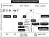 |
Fig. 1 CSI SN classification scheme. Viable SN explosion mechanisms, the main elements in their spectra, their light curve properties (only for SN IIn subtypes), the degree of association (NCR) to H ii regions (only for SN IMs) and the possible progenitors are shown in correspondence with their CSI SN subtype. |
There is indeed evidence that at least some SNe IIn arise from LBVs. Gal-Yam et al. (2007) identified a likely LBV in pre-explosion images at the location of SN IIn 2005gl. SN 2009ip exhibited LBV-like outbursts before the last major event, which might be explained with its CC (Prieto et al. 2013; Mauerhan et al. 2013a; Smith et al. 2014). For several SNe IIn from the Palomar Transient Factory (PTF), there is evidence of stellar outbursts before their terminal endpoint (Ofek et al. 2014). Furthermore, the CSM velocities observed in SNe IIn are often consistent with those expected for LBV winds (~100–1000 km s-1), and the large mass-loss rates observed in SNe IIn are also compatible with those of large LBV eruptions, ranging between 10-3 and 1 M⊙ yr-1 (Kiewe et al. 2012; Taddia et al. 2013a; Moriya et al. 2014). The presence of bumps in the light curves of some SNe IIn can also be understood as the SN ejecta interaction with dense shells produced by episodic mass-loss events (e.g., SN 2006jd, S12). In summary, there is thus ample observational evidence from different lines of reasoning that connect LBVs and SNe IIn.
However, red supergiant (RSG) stars with superwinds (e.g., VY Canis Majoris) also have been proposed to be progenitors of long-lasting SNe IIn (see, e.g., SN 1995N, Fransson et al. 2002; Smith et al. 2009a), since they are characterized by strong mass loss forming the CSM needed to explain the prolonged interaction.
There are other SNe IIn that fade faster than the aforementioned 1988Z-like SNe. These events have early decline rates of ~2.9 mag (100 days)-1, and given the linear decline in their light curves, they can be labeled Type IIn-L SNe.
Among the SNe IIn-L, it is possible to make further subclassifcations based on their spectra. Some SNe IIn-L show slowly evolving spectra (e.g., SNe 1999el, Di Carlo et al. 2002, 1999eb; Pastorello et al. 2002), with narrow emission lines on top of broad bases lasting for months. Other SNe IIn-L display spectra with a faster evolution, with Type IIn-like spectra at early times and Type IIL-like spectra (broad emission lines, sometimes broad P-Cygni absorption) at later epochs (e.g., SN 1998S, Fassia et al. 2000, 2001; and SN 1996L, Benetti et al. 2006). The different spectral evolution of these two subtypes can be traced back to the efficiency of the SN-CSM interaction and to different wind properties. Also for SNe IIn-L, both LBV (e.g., Kiewe et al. 2012) and RSG (e.g., Fransson et al. 2005) progenitors have been considered in the literature.
Both LBVs and RSGs could be responsible for the production of CSI SNe when they are part of binary systems. We have already discussed the mechanism proposed by Smith & Tombleson (2015) for LBVs. Mackey et al. (2014) explain how interacting supernovae can come from RSGs in binary systems. In their scenario, the binary companion of a RSG can photoionize and confine up to 35% of the gas lost by the RSG during its lifetime, forming a dense CSM close to the RSG star itself. When the RSG explodes, the SN appears as a CSI SNe, as the SN ejecta interact with this dense shell.
Mauerhan et al. (2013b) suggested the name “IIn-P" for objects resembling SN 1994W, i.e., SNe with Type IIn spectra showing a ~100 days plateau in the light curve, similar to that of SNe IIP, followed by a sharp drop and a linear declining tail at low luminosity. The nature of these events is currently debated; some authors have proposed that 1994W-like SNe arise from the collision of shells ejected by the progenitor star and not from its terminal explosion (e.g., Humphreys et al. 2012; Dessart et al. 2009). However, for SN 2009kn a bonafide CC origin was favored by the observations of Kankare et al. (2012). Others even suggested SN 1994W was the result of a fall-back SN creating a black hole (Sollerman 2002) and it has also been proposed that SNe IIn-P might be electron-capture (EC) SNe (Nomoto 1984) coming from the explosion of super asymptotic giant branch (AGB) stars (e.g., Chugai et al. 2004; Mauerhan et al. 2013b).
An additional member of the family of SNe IIn are the so-called superluminous SNe II (SLSNe II). These objects reach peak absolute magnitude of <−21 mag (Gal-Yam 2012), and SN 2006gy serves as the prototypical example (Smith et al. 2007). The mechanism powering these bright transients could be something different from CSM interaction, such as radioactive decay of large amounts of 56Ni or energy from a magnetar. We do not focus on the host galaxies of SLSNe II with the exception of SN 2003ma, which shows a light curve shape similar to that of SN 1988Z but brighter by ~2.5 mag (Rest et al. 2011).
Besides SNe IIn, in the CSI SN group we also find the so-called SNe Ibn, or 2006jc-like SNe (e.g., Matheson et al. 2000; Foley et al. 2007; Pastorello et al. 2007, 2008a,b; Smith et al. 2008a; Gorbikov et al. 2014). These are transients showing He emission lines, arising from the SN interaction with a He-rich CSM. These SNe likely originate from the explosion of massive WR stars. The WR progenitor SN 2006jc was observed to outburst two years before the SN explosion.
Another class of objects arising from CSM interaction is the Type Ia-CSM or 2002ic-like subgroup. These events are interpreted as thermonuclear SNe interacting with H-rich CSM (Hamuy et al. 2003; Aldering et al. 2006; Dilday et al. 2012; Taddia et al. 2012; Silverman et al. 2013; Fox et al. 2015), although a CC origin has also been proposed (Benetti et al. 2006; Inserra et al. 2014). Their spectra are well represented by the sum of narrow Balmer emission lines and SN Ia spectra diluted by a blue continuum (Leloudas et al. 2015b).
Finally, a class of transients resembling SNe IIn is that of the SN impostors (SN IMs). These events are the result of outbursts from massive stars. Most of the information regarding the observables of SN IMs has been collected by Smith et al. (2011a, see their Table 9). In Smith et al. (2011a) SN IMs are interpreted as the result of LBV eruptions. Some LBVs may be observed in the S-Doradus variability phase (e.g., the 2009 optical transient in UGC 2773; Smith et al. 2010, 2011a; Foley et al. 2011). LBVs in the S-Doradus phase are typically characterized by a variability of 1–2 visual magnitudes, usually interpreted as the result of a temperature variation at constant bolometric luminosity (Humphreys & Davidson 1994). Occasionally even giant eruptions of LBVs similar to that observed in Eta-Carinae during the 19th century may be observed in external galaxies (e.g., SN 2000ch, Wagner et al. 2004; Pastorello et al. 2010). Their typical luminosities are lower than those of SNe IIn (M > −14), even though some bright events are now suspected to belong to this class (e.g., SN 2009ip, Pastorello et al. 2013; Fraser et al. 2013; Margutti et al. 2014). Among SN impostors, objects like SN 2008S have been proposed to be electron-capture SNe from super-AGB stars rather than LBV outbursts (e.g., Botticella et al. 2009; see Sect. 7.3).
1.2. This work
An approach to investigate whether the LBVs, which produce (at least some) SN IMs, are the dominant progenitor channel for SNe IIn is to compare the properties of the environments of SNe IIn and SN IMs. In particular, the metallicities of the surrounding material can be measured via strong emission-line diagnostics. This is the focus of this paper.
If the vast majority of SNe IIn originate from LBVs associated with SN IMs, then the metallicity distributions of these two groups should be similar. If these distributions do not match, there could be room for other progenitor channels of SNe IIn. Metallicity measurements of SNe IIn and SN IMs, based on the host-galaxy absolute magnitudes, are provided by H14. We provide local metallicity estimates for a large sample of CSI transients, including SNe IIn, Ibn, Ia-CSM, and SN IMs. Our measurements, carried out on data obtained at the Nordic Optical Telescope (NOT), are complemented with data available in the literature (e.g., Kelly & Kirshner 2012, hereafter KK12, and H14) and in public archives.
Metallicity measurements at the locations of CSI transients are important to compare the environments of SNe IIn and SN IMs, and to clarify the role of metallicity in the prevalent mass losses of these events. It is well known that, given a certain stellar mass, a higher metallicity drives a larger mass loss in massive stars, due to stronger line-driven winds (e.g., Kudritzki & Puls 2000). However, the mass-loss rates due to this mechanism, observed in hot stars like WR, are on the order of 10-5M⊙ yr-1, which is substantially lower than what is required in SNe IIn. The massive CSM around SNe IIn must be produced by larger eruptions, whose underlying mechanism and metallicity dependence is largely unknown (e.g., gravity waves and super-Eddington winds have been invoked, Quataert & Shiode 2012; Smith et al. 2006). Since the mass loss of SN IIn progenitors and SN IMs shapes their CSM and thus the appearance of these transients, by looking for correlations between metallicity and observational properties of these transients, we aim to constrain to what extent metallicity is an important ingredient. We collected the observables available in the literature for each SN with measured metallicity at its explosion location. We also complemented our analysis of the metallicity with that of another important property related to the SN environment, which is the association of SN locations to star-forming (SF) regions. In doing that, we used the results published by H14.
The paper is organized as follows. In Sect. 2 we introduce our SN sample, and Sect. 3 presents our observations and data reduction procedures. Section 4 describes how we subtracted the underlying stellar population from each spectrum, how we measured the emission line fluxes, and the spectral classification. Section 5 concerns the method to obtain the local metallicity measurements, and Sect. 6 presents the results on the metallicities of CSI SNe, which are compared among the different CSI SN subtypes and with those of other CC SN classes. In Sect. 7 we show the relations between metallicity and observables of CSI SNe, and, finally, the discussion and conclusions are given in Sect. 8 and 9, respectively.
2. Sample of CSI transient host galaxies
In Table 1 we report the list of 60 transients included in our sample. Thirty-five of them are SNe IIn, six are SNe Ibn, one is a SN Ia-CSM, 18 are SN IMs (if we also count SN 2009ip in the SN IMs, then we have 19 of these transients).
With the NOT, long-slit spectra were obtained for the host galaxies of 13 SNe IIn, five SNe Ibn, one SN Ia-CSM, and 16 SN IMs (the derived metallicity for SN 2007sv was published in Tartaglia et al. 2015). The host galaxies observed at the NOT are marked with the letter “o" in the third column of Table 1. With the NOT, we also obtained broad-band R and narrow-band Hα images for the SNe IIn (except for SN 1995G) and Ibn.
Metallicity estimates and normalized cumulative rank (NCR) pixel index for the sample of CSI transients.
The CSI transients observed at the NOT were chosen among those with published spectroscopic and photometric data. These SNe were thoroughly analyzed in the literature (e.g., Kiewe et al. 2012; Taddia et al. 2013a, and references in Tables 5 and 7), and, for most of these objects, estimates of the physical properties of the CSM, such as wind velocity and mass-loss rate, were also available. We made this choice to select objects whose observational and physical properties could be related to their host galaxy properties, such as the metallicity (see Sect. 7). In particular, SN IMs were chosen among those listed by Smith et al. (2011a). We also decided to observe nearby, i.e., resolved, host galaxies (z< 0.026, see Table 1) to allow for the determination of the local metallicity. We discuss the possible biases introduced by this selection in Sect. 8.
We complemented our observed sample with host galaxies whose metallicities (at the center of the galaxy or at the SN position) were already available in the literature (marked with the letter “l" in the third column of Table 1) or whose spectra were available in public archives (marked with the letter “a" in the third column of Table 1). Eighteen SNe IIn (excluding SNe 2005ip and 2006jd) have metallicities published in the literature (mainly from KK12 and H14) and four have host-galaxy spectra obtained by the 6dF survey (Jones et al. 2009) and available via NED1. For two SNe Ibn, their host-galaxy spectra are available in public archives. Metallicity measurements were available in the literature for nine SN IMs (excluding SN 2007sv that we already published, and including SN 2009ip) and for six of them we also obtained observations at the NOT. Most of the metallicity estimates for SN IMs in the literature were obtained from P04. All the references are reported in Table 4 (4th column). In summary, our entire sample includes a large fraction of the CSI SNe with published light curves and spectra.
Considering the entire sample, on average SN IMs are located at lower redshift (⟨ zIM ⟩ = 0.0020 ± 0.0004) compared to SNe IIn (⟨ zIIn ⟩ = 0.0276 ± 0.0092) and Ibn (⟨ zIbn ⟩ = 0.0216 ± 0.0078), since most of them were only discovered in nearby galaxies because of their lower luminosity.
3. Observations and data reduction
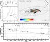 |
Fig. 2 Top right panel: continuum-subtracted Hα image of UGC 4286, the host galaxy of SN 2010al. The 25th B-band magnitude elliptic contour is shown with a black solid line, along with the position of SN 2010al (marked by a red star) and the center of the galaxy (marked by a red circle). The slit position is shown, and a color code is used to present the N2 metallicity measurements at the position of each H ii region that we inspected. Top left panel: flux at the Hα wavelength along the slit, shown as a function of the distance from the SN location (marked by a dotted line, like the nucleus position). The N2 measurements are shown at the corresponding positions in the top subpanel. Bottom panel: metallicity gradient of UGC 4286. The linear fit on our measurements is shown with a solid line. The interpolated metallicity at the SN distance is marked with a red square and its uncertainty corresponds to the fit error. The error bar (±0.2) for our N2 measurements is shown aside. The positions of SN and nucleus are marked with vertical dotted lines. The solar metallicity (Asplund et al. 2009) and the LMC metallicity (Russell & Dopita 1990) are indicated with two horizontal dotted lines. |
3.1. Nordic optical telescope observations and data reduction
We performed observations at the NOT and data reductions following the procedures outlined in Taddia et al. (2013b), where we studied the host galaxies of SN 1987A-like events arising from the explosions of blue supergiant stars (BSGs). In this section, we provide a brief summary of how we obtained and reduced our visual-wavelength spectroscopy.
Two observational campaigns (P45-004, P49-016) were carried out during 2012 and 2014. Six nights were spent observing the hosts of SNe IIn, Ibn, and Ia-CSM in 2012 (four in April, one of which was lost to bad weather, and two in September). Four nights were spent observing the host galaxies of SN IMs (three in April 2014, one in September 2014). During April 2014, almost 1.5 of the three nights were lost to bad weather.
In both campaigns our main goal was to determine the metallicity at the exact position of the CSI transients through strong emission-line diagnostics. To accomplish this, we obtained long-exposure (≳1800 s), long-slit spectra of the star forming (H ii) regions within the host galaxies, by simultaneously placing the slit at the SN position and through the galaxy center or through bright H ii regions near the SN location. To intercept both the host galaxy center (or bright H ii regions) and the SN location with the slit, we rotated the telescope field by the corresponding angle; then, the slit was centered on a pre-determined reference star in the field and, finally, the telescope was offset to point to the SN location. The final pointing was checked with a through slit image. In most cases the slit included a few H ii regions, allowing for a determination of the host galaxy metallicity gradient and hence of the metallicity at the distance of the SN from the host center (see Sect. 5).
The instrumental setup that was chosen to acquire the host galaxy spectra at the NOT was the same as adopted for the study presented in Taddia et al. (2013b), i.e. ALFOSC with grism #4 (wide wavelength range ~3500−9000 Å) and a 1.0″-wide slit (corresponding to the typical seeing on La Palma). The obtained spectral resolution is ~16–17 Å. The exposure times adopted for each spectral observation are listed in Table 2.
The following procedure was adopted to carry out the spectral reductions. First, the 2D spectra were bias subtracted and flat-field corrected in a standard way. When available, multiple exposures were then median-combined to remove any spikes produced by cosmic rays. We extracted the trace of the brightest object in the 2D spectrum (either the galaxy nucleus, a bright star, or a H ii region with a bright continuum) and fitted with a low-order polynomial. The precision of this trace was checked by plotting it over the 2D spectrum. We then shifted the same trace in the spatial direction to match the position of each H ii region visible in the 2D spectrum, and then extracted a 1D spectrum for each H ii region. The extraction regions were chosen by looking at the Hα flux profile, an example of which is presented in the top-left panel of Fig. 2, where we also report the width of each spectral extraction. The extracted spectra were wavelength and flux calibrated using an arc-lamp spectrum and a spectrophotometric standard star observed the same night, respectively. Following Stanishev (2007), we removed the second order contamination, which characterizes the spectra obtained with grism #4, from each spectrum. In this study, we included all the spectra showing at least Hα, [N ii] λ6584 and Hβ emission lines. We identified the location of each corresponding H ii region by inspecting the acquisition images.
For SNe IIn, Ibn, and Ia-CSM, we also had the chance to observe the host galaxies in a narrow Hα filter and a broad R-band filter, to build Hα maps, as detailed in Taddia et al. (2013b). These maps further helped us to precisely determine the location of each H ii region that was spectroscopically observed. An example of a continuum-subtracted Hα images is shown in the top-right panel of Fig. 2. Here we indicate the SN position with a red star and the galaxy nucleus with a circle. An ellipse marks the 25th B-band magnitude contour. Each colored patch within the plotted slit aperture corresponds to the position of an extracted H ii region spectrum. We also attempted to use these Hα maps to measure the degree of association (NCR, see Sect. 7.3) to H ii regions for each SN. However, since we had to cut the exposure times because of bad weather, we did not reach the desired depth in the Hα images. The time lost because of bad weather in the 2014 campaign also prevented us from obtaining the same photometric observations for the host galaxies of SN IMs. However, we used NCR data from H14 in the discussion about the SN IIn progenitor scenarios (see Sect. 8.1). Table 2 summarizes all the observations carried out during the two campaigns.
3.2. Archival data
We used archival spectra to complement the data set for SNe IIn and Ibn. All four spectra retrieved via NED are low-resolution spectra obtained at the galaxy center by the 6dF Galaxy Survey (Jones et al. 2009). The spectrum of LSQ12btw was retrieved via the ESO archive and reduced. All these spectra included at least Hα, [N ii] λ6584, and Hβ emission lines.
 |
Fig. 3 Top panel: STARLIGHT stellar-population spectrum best fit to the continuum of the spectrum obtained at the center of the host galaxy of SN 2006aa. The difference between the observed spectrum and the best fit gives the pure emission-line spectrum. Bottom panel: the triple-Gaussian fit on the continuum-subtracted Hα and [N ii] lines of the bright H ii region at the center of the host galaxy of SN 2006aa. The observed fluxes are represented with black crosses, the best fit in red, the Hα component in blue, and the [N ii] components in green. |
4. Stellar population subtraction, line measurements, and spectral classification
To accurately measure the emission line fluxes necessary to determine the metallicity, the stellar population component of each spectrum was modeled with the STARLIGHT code (Cid Fernandes et al. 2005)2 and subtracted from each observed spectrum (corrected for the Galactic extinction). This code linearly combines synthetic spectra from Bruzual & Charlot (2003) and takes dust attenuation into account to fit the emission-line free regions of our spectra. The template spectra are stellar population spectra at 15 different ages between 0.001 and 13 Gyr and three metallicities (Z = 0.2, 1, 2.5 Z⊙). The same templates were used by Leloudas et al. (2011) in their study of SNe Ib/c locations. As an example, the best fit to the spectral continuum of SN 2006aa host galaxy nucleus is shown in Fig. 3 (top panel), as well as the “pure” emission line spectrum, as obtained from the observed spectrum subtracted of the best-fit continuum. Once we obtained the pure emission line spectra, we proceeded to measure the fluxes of [N ii] λ6584 and Hα, Hβ, and [O iii] λ5007.
To measure the fluxes of the [N ii] λ6584 and Hα emission lines, we followed a fitting procedure similar to that outlined in Taddia et al. (2013b). Given the low resolution of our ALFOSC spectra, we had to deblend [N ii] λ6584, [N ii] λ6548, and Hα through a triple Gaussian fit. We fixed the width of each Gaussian to be the same, as determined by the spectral resolution. The known wavelength offsets between the centroids of the three lines was also fixed. The flux of [N ii] λ6548 was furthermore fixed to be 1/3 of that in [N ii] λ6584 (see Osterbrock & Ferland 2006). This assumption was needed to allow for a proper fit of this faint line, which could possibly contaminate the flux of Hα. Finally, the integrals of the two Gaussians, fitted to [N ii] λ6584 and Hα, provided us with the fluxes of these lines (see the bottom panel of Fig. 3 for an example of the fitting procedure). For each spectrum we measured the Hβ and [O iii] λ5007 line fluxes by fitting them with Gaussians. In several cases we could only place a limit on the flux of [O iii] λ5007.
The ratios of line fluxes, such as F([N ii] λ6584) to F(Hα), and F([O iii] λ5007) to F(Hβ), can be used to determine the metallicity only if the dominant ionizing source for each region are hot massive stars, since strong line diagnostics are based on this condition. To exclude other possible ionizing sources, such as shock-excitation or AGN contamination, we classified our spectra based on the BPT diagram (Baldwin et al. 1981), which shows log 10(F([O iii] λ5007)/F(Hβ)) versus log10(F([N ii] λ6584)/F(Hα)), which is widely used to discriminate between the excitation sources of emission line objects. Gas ionized by different sources occupies different areas across the BPT diagram (e.g., Kewley et al. 2001; Kehrig et al. 2012; Sánchez et al. 2014; Galbany et al. 2014; Belfiore et al. 2015). In Fig. 4 we plot log10(F([O iii] λ5007)/F(Hβ)) versus log10(F([N ii] λ6584)/F(Hα)) for our spectra and checked if these points were located within the BPT diagram area given by Kauffmann et al. (2003), i.e., log 10(F([O iii] λ5007)/F(Hβ)) < 0.61 / (log 10(F([N ii] λ6584)/F(Hα))−0.05) + 1.3, which defines the star-forming galaxies as opposed to galaxies with AGN contamination. The line ratios for each H ii region are reported in Table 3. We rejected the spectra falling in the other region of the BPT diagram. This occurred for the nuclear spectra of the host galaxies of SNe 1994W, 1995G, 2001ac, 2005dp, and 2005gl, and for another region of the hosts of SNe 2001ac and 1997bs. We also excluded the hosts of SNe 1996L (Benetti et al. 1999), 2005kj (Taddia et al. 2013a), and iPTF11iqb (Smith et al. 2015) from our sample as we only had a nuclear spectrum with log10(F([O iii] λ5007)/F(Hβ)) > 0.61/(log10(F([N ii] λ6584)/F(Hα))−0.05) + 1.3.
For the objects falling in the general locus of H ii regions-like spectra, we use N2 [=log10(F([N ii] λ6584)/F(Hα))] to derive the metallicities (see Sect. 5).
5. Oxygen abundances at the SN explosion sites
In this section we describe how the metallicity at the SN location was estimated from the observed and archival spectra after stellar population subtraction, line fitting, and spectral classification. We also show how we included the metallicity values available in the literature. For the observed spectra, we followed the procedure illustrated in Taddia et al. (2013b).
5.1. Local metallicity measurements from observed and archival spectra
Among the possible emission line diagnostics, we chose to use N2 (Pettini & Pagel 2004) for all our metallicity measurements. The oxygen abundance can be obtained from N2 using the following expression presented by Pettini & Pagel (2004):  This expression is valid in the range −2.5 <N2 < −0.3, which corresponds to 7.17 < 12 + log (O / H) < 8.86. This method has a systematic uncertainty of 0.18, which largely dominates over the error from the flux measurements. Following Thöne et al. (2009) and Taddia et al. (2013b), we adopted 0.2 as the total error for each single measurement. Marino et al. (2013) recently revised the N2 index using a large data set of extragalactic H ii regions with measured Te-based abundances. However, we use the calibration by Pettini & Pagel (2004) to allow for a direct comparison with other SN types (see Sect. 6.2).
N2 has a larger systematic uncertainty than other methods, such as O3N2 (Pettini & Pagel 2004). However, N2 presents several advantages that are briefly summarized here. 1) For nearby galaxies, the lines needed for this method fall in the part of the CCD with higher efficiency and thus are easier to detect than those needed for the other methods (e.g., O3N2 and R23, where lines in the blue or in the near ultraviolet are required). 2) Given that Hα and [N ii] λ6584 are very close in wavelength, this minimizes the effects associated with differential slit losses (we did not observe at the parallactic angle as we placed the slit along the SN location – host-galaxy center direction) and uncertainties on the extinction. 3) It is well known that there are non-negligible offsets between different line diagnostics (Kewley & Ellison 2008), and as N2 was used to estimate the metallicity for many other SNe in the literature (e.g., Thöne et al. 2009; Anderson et al. 2010; Leloudas et al. 2011; Sanders et al. 2012; Stoll et al. 2013; Kuncarayakti et al. 2013a,b; Taddia et al. 2013b), this method allows for a direct comparison of CSI transients to other SN types (see Sect. 6.2).
There are possible drawbacks when using N2. For instance, the existence of a correlation between the metallicity derived from the N2 parameter and the N/O ratio (Pérez-Montero & Contini 2009) together with the presence of N/O radial gradients across the disks of spiral galaxies (see, e.g., P04; Mollá et al. 2006) can affect the metallicity measurements obtained with this method. The most precise method to determine the oxygen abundances would be via the weak [O iii]λ4363 line flux (see, e.g., Izotov et al. 2006), but we could not detect this line in our spectra.
For each H ii region with measured N2 metallicity and [O iii] λ5007/Hβ) < 0.61 / (N2–0.05) + 1.3, and for each SN, we computed their deprojected and normalized distance from their host-galaxy nuclei, following the method illustrated by Hakobyan et al. (2009, 2012).
To accomplish this, we established the coordinates of the H ii region/SN, and collected all the necessary information about its host galaxy: nucleus coordinates, major (2 R25) and minor (2b) axes, position angle (PA), and morphological t-type. All these data, with the corresponding references, are listed in Table 1, which also reports the result for the deprojected distance of each SN, rSN/R25. We mainly used NED to collect the SN and galaxy coordinates as well as the galaxy dimensions and position angle. The Asiago Supernova Catalogue3 (ASC) was used for the t-type, and SIMBAD4 and HYPERLEDA5 were used when neither NED nor ASC included the aforementioned galaxy data.
Having obtained the distance from the nucleus for each H ii region (see the first column of Table 3), we plotted their metallicities versus these distances and performed a linear chi-square fit to the data. An example of this fit is reported in the bottom panel of Fig. 2. In most cases, the metallicity was found to decrease as the distance from the center increases (with the exception of nine hosts, where flat or positive gradients were derived). It is well known that there is a negative metallicity gradient in galaxies (e.g., P04), likely because the star formation rate depends on the local density and therefore more metals have been produced in the denser, central parts of the galaxies. All the data and the fits are shown in Figs. 5–7.
The linear fits allowed us to interpolate or extrapolate the metallicity at the computed SN distance from the host center (see, e.g., the red square in the bottom panel of Fig. 2). These values were taken to be the local SN metallicity estimate. These estimates were always found to match the metallicity of the H ii region closest to the SN. In this way, we also provided oxygen abundances for those SNe that were not associated with a bright H ii region (this is the case of several SN IMs, see Sect. 7.3), and for those SN IMs or SNe IIn whose flux was still dominating the emission (e.g., SN IM 2000ch). All the local and central metallicities, and the metallicity gradients are reported in Table 4.
When more than two H ii regions were observed, we computed the uncertainty on the interpolated/extrapolated SN metallicity as the standard deviation of 1000 interpolation/extrapolations of 1000 Monte Carlo-simulated linear fits, based on the uncertainty on the slope and on the central metallicity. These uncertainties are those reported in Table 4 and do not include the systematic N2 error (see Taddia et al. 2013b for a motivation of this choice). When only two measurements were obtained, we assumed 0.2 as the uncertainty for the metallicity at the SN position and at the host center.
For most of the galaxies whose spectra were retrieved from online archives, only a single measurement was possible, often at the host center. In these cases, we adopted a standard metallicity gradient (–0.47  ) to extrapolate the metallicity at the SN position. This value corresponds to the average gradient of the large galaxy sample studied by P04. In these cases the error on the SN metallicity included the extrapolation uncertainty, given by the ~0.1 dispersion of the measured metallicity gradients (see Sect. 6.1).
5.2. Local metallicity values from the literature
In the literature we found several published values for the metallicities of CSI SN host galaxies. Some of them were local (e.g., a few from H14), most of them were measurements at the host galaxy center (e.g., all those obtained by KK12, except that of the host of SN 1994Y). KK12 presented O3N2 metallicity estimates based on SDSS spectral measurement performed by an MPA-JHU collaboration and available online6. Therefore we retrieved the needed line fluxes for the N2 method for all the SN IIn hosts presented by KK12 and computed the metallicity measurements in the N2 scale. H14 and Roming et al. (2012) present five O3N2 values, so we had to convert them to the N2 scale, using the relation presented by Kewley & Ellison (2008). In the cases where the metallicity was measured at the host nucleus, we assumed the aforementioned standard gradient to obtain the metallicity at the SN deprojected distance. We could have used the average gradient that we measured in some of our galaxies (see Sect. 6), instead of the average gradient from P04. However, the sample of galaxies observed by P04 is larger and representative of many morphological types, so we prefer to adopt their value. This assumption could potentially affect the results concerning SNe IIn (for 13 of the 35 SNe IIn we adopt the P04 average gradient), whereas it is not important for most of the SN IMs or SN Ibn, for which we do not need to assume any average gradient. However, we show in the following sections that the SN IIn results are solid independent of the average gradient assumption.
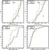 |
Fig. 8 Top left panel: cumulative distribution functions (CDFs) of the central metallicities for SN IIn, Ibn, and SN IM host galaxies. SN Ibn and SN IM hosts show slightly lower metallicities than SN IIn hosts. Top right panel: CDFs of the metallicity at the SN location for the same three classes. SN IMs and SNe Ibn are located in lower metallicity environments than those of SNe IIn. Bottom panels: CDFs of the host metallicity gradients and deprojected SN distances from the host center for SNe IIn, Ibn, and SN IMs. |
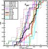 |
Fig. 9 CDFs of the metallicity at the SN location for CSI transients and for other SN classes from the literature. We ordered the legend entries by mean metallicity. |
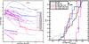 |
Fig. 10 Left-hand panel: SN IIn light curves from the literature. Three main subclasses are identified (plus the SLSNe) based on the light curve shape. Long-lasting SNe IIn (1988Z-like; blue) show slow decline (~0.7 mag (100 days)-1) and sustained luminosity for ≳5 months. SN IIn-P (1994W-like; red) show a ~3–4 month plateau followed by a sharp drop, similar to what is observed in SNe IIP. SNe IIn-L (1998S or 1999el-like, depending on the spectral evolution; magenta) show a faster decline (~2.9 mag (100 days)-1). References for the light curve data and the extinction of SNe with measured metallicity can be found in Table 5. For SNe 1994aj, 1999el, 2005cl, 2006gy, 2006tf, and 2009kn, the references are Benetti et al. (1998), Di Carlo et al. (2002), Kiewe et al. (2012), Smith et al. (2007), Smith et al. (2008b), and Kankare et al. (2012), respectively. Right-hand panel: CDFs of the metallicity at the SN location for our CSI transients, including three SN IIn subclasses (1988Z-like, 1994W-like, 1998S-like). 1998S-like SNe are located at higher metallicity compared to the other subtypes. |
6. Metallicity results
In the following sections, we describe the metallicity results for our sample of CSI transients, including comparisons among CSI SN subtypes and to other CC SNe.
6.1. Metallicity comparison among CSI transients
In Table 4 we report the average values for the metallicity at the host center, at the SN position, and for the metallicity gradient. The mean gradients are computed excluding the objects where the gradient was assumed to be –0.47 .
SNe IIn show slightly higher average oxygen abundance at their locations (8.47 ± 0.04) than do SN IMs (8.33 ± 0.06). The latter values are consistent with the metallicity of the Large Magellanic Cloud (LMC has 8.37, Russell & Dopita 1990), which is subsolar (the Sun has 8.69, Asplund et al. 2009). To understand if this difference is statistically significant, computing the mean values is not sufficient. Therefore, we need to compare their cumulative distributions, which are shown in the top-right panel of Fig. 8, through the Kolmogorov-Smirnov (K-S) test. We found that the probability that the metallicity distributions of SNe IIn and SN IMs are different by chance is only 1%. If we exclude the CSI SN hosts where we assumed the average P04 metallicity gradient to determine the local oxygen abundance, this difference still holds (p-value =1.5%), with ⟨ 12 + log (O / H) ⟩ IIn = 8.48 ± 0.04 and ⟨ 12 + log (O / H) ⟩ IM = 8.31 ± 0.07. Also if we use the N2 calibration by Marino et al. (2013), the K-S test gives a p-value of 1%. To account for the uncertainties of each metallicity measurement (see Table 4), we performed the K-S test between 106 pairs of Monte Carlo-simulated metallicity distributions of SNe IIn and SN IMs. The 68% of the resulting p-values were found to be ≤0.17, indicating that the difference is real. We discuss this result and its implications for the SN IIn progenitor scenario in Sect. 8. SNe Ibn show an average metallicity (8.44 ± 0.11) similar to that of SNe IIn and a distribution that appears in between those of SNe IIn and SN IMs, although here our sample is limited to only six SNe Ibn and there is no statistically-significant difference with the other two distributions (p-values >56%).
The average oxygen abundances at the host center for SNe IIn and SN IMs are 8.63 ± 0.03 and 8.59 ± 0.06, respectively. These distributions (top-left panel of Fig. 8) turned out to be similar, with p-value =47%. SN Ibn hosts exhibit a slightly lower mean central metallicity than SNe IIn (8.55 ± 0.11, but with p-value =54%). Metallicities at the center are expected to be higher than those at the SN explosion site because of the negative metallicity gradient typically observed in the galaxies (e.g., P04).
The mean gradient for the host galaxies of SNe IIn, Ibn, and SN IMs is  ,
,  and
and  , respectively. These absolute values are slightly lower than the average gradient (
 ) of the galaxies studied by P04 and adopted for the SNe in our sample with a single metallicity estimate at the galaxy center. The gradient distribution of SN IIn hosts shows higher values than those of SN IMs and SNe Ibn (bottom-left panel of Fig. 8), however, the K−S tests result in p-values >12%.
SNe IIn, Ibn, and SN IMs show similar average distances from the host center, with 0.64 ± 0.15 R25, 0.43 ± 0.10 R25, and 0.54 ± 0.08 R25, respectively. Their distributions are almost identical (p-values >49%, see the bottom-right panel of Fig. 8).
If we had assumed our average metallicity gradient instead of that from P04 for the hosts with a single measurement at the center, then the metallicity distribution of SNe IIn (which is the only one that would be affected by a different choice of the average metallicity gradient) would have been at slightly higher metallicity, making the difference with SN IMs even more significant.
6.2. Metallicity comparison to other SN types
Figure 9 shows the cumulative distributions of the metallicity at the SN location for our CSI transients, along with those of other SN types previously published in Taddia et al. (2013b, see Fig. 15 and references in the text) and Leloudas et al. (2015a). All the metallicities included in the plot are local and obtained with the N2 method to enable a reliable comparison among the different SN classes. It is evident that the SN IMs have relatively low metallicities along with SN 1987A-like events, SNe IIb, and SLSN II. When we compare the metallicity distribution of SN IMs to that of SNe IIP, their difference has high statistical significance (p-value =0.09%; even higher if the comparison is to SNe Ibc). SNe IIn show higher metallicities than SN IMs, but still lower than those of SNe IIP (p-value =29%) and SNe Ibc (p-value =2.5%, highly significant). All the SN types show higher metallicities compared to SLSNe I and SLSNe R.
7. Host galaxy properties and CSI transient observables
In the following sections, we investigate any potential correlations between the observables of CSI transients and the properties of their environment, in particular the metallicity. This exercise aims to establish to what extent metallicity plays an important role in shaping the appearance of these events.
7.1. Metallicity and SN properties
7.1.1. Metallicity and SN IIn subtypes
In the introduction we described three SN IIn subgroups, mainly based on the light curve shapes, i.e., 1988Z-like (or long-lasting SNe IIn), 1994W-like (or SNe IIn-P), and 1998S-like (or SNe IIn-L with fast spectral evolution). A collection of SN IIn light curves from the literature, including most of the light curves of SNe IIn with measured metallicity, is shown in Fig. 10 (left-hand panel), where we show the different subtypes in different colors. In our sample we selected the events belonging to the different SN IIn subclasses (see the second columns of Tables 5–7) to look for possible trends in the metallicity. In Fig. 10 (right-hand panel) we plot their metallicity CDF. It was possible to subclassify only 21 of the 35 SNe IIn in our sample, i.e., those with sufficient photometric coverage in the literature. We found that our SN IIn-L (we only have 1998S-like SNe) are typically located at solar metallicity (⟨ 12 + log (O / H) ⟩ IIn − L = 8.69 ± 0.03). Long-lasting SNe IIn are found at lower metallicity (⟨ 12 + log (O / H) ⟩ IIn−88Z = 8.38 ± 0.06), similar to SN IMs. Among them, the object showing the largest oxygen abundance is SN 2005ip. The difference between SN 1998S-like events and long-lasting SNe IIn is statistically significant (p-value =0.004), and would be even larger if we had adopted our measured average metallicity gradient instead of that from P04, since we assumed the P04 gradient for the hosts of three (out of five) SNe IIn-L. It would also be statistically significant if we exclude the hosts where we assumed the P04 gradient from both groups. 1994W-like SNe exhibit a metallicity distribution similar to that of 1988Z-like SNe (⟨ 12 + log (O / H) ⟩ IIn − P = 8.39 ± 0.12). In this group we include only SNe 1994W, 2006bo, and 2011ht, which do show a plateau followed by a sharp decay.
7.1.2. Metallicity and SN IIn/Ibn magnitude at peak
It has been noticed in the literature that some bright SNe IIn exploded in low-metallicity environments (Stoll et al. 2011). We have the opportunity to test if this kind of trend can be confirmed for a larger sample of SNe IIn. For each CSI SN, we collected their peak apparent magnitudes in five optical bands (U/u, B, V, R/r/unfiltered, I/i) when available in the literature. We also collected the visual Galactic extinction for each SN (AV(MW), from Schlafly & Finkbeiner 2011) and, when available in the literature, an estimate of the host extinction (AV(h)).
Peak magnitudes and extinctions are summarized in Table 5, with references provided. We computed the distance from the redshift (see Table 1), assuming H0 = 73.8 km s-1 Mpc-1 (Riess et al. 2011). Using the distance and the extinction estimate, we computed the absolute peak magnitude (Mu/U,B,V,R/r/unf.,I/i) from the apparent peak magnitude of each filter. These magnitudes are reported in Table 6 and plotted against the local metallicity estimates in Fig. 11. When the absolute peak magnitude is only an upper limit, it is marked with a triangle. This figure does not show any clear correlation or trend between metallicity and luminosity at peak. When we group our events in different metallicity bins (i.e., log(O/H)+ 12 ≤ 8.2,8.2 < log (O / H) + 12 ≥ 8.4, 8.4 < log (O / H) + 12 ≥ 8.6, log (O / H) + 12 > 8.6) and compare their absolute magnitude distributions via K−S tests, no statistically significant difference is found. We thus see no evidence that normal SNe IIn exhibit brighter absolute magnitudes at lower metallicities. However, we note that SLSNe II (Mr/R< −21), which might also be powered by CSI, are typically found at lower N2 metallicities (8.18 < log (O / H) + 12 > 8.62) than those of our normal SN IIn sample (Leloudas et al. 2015a).
7.1.3. Metallicity and dust emission
Fox et al. (2011) observed a large sample of SNe IIn at late epochs in the mid-infrared (MIR) with Spitzer. Among their SNe IIn, 17 events are included in our sample and six of them show dust emission (including SN 2008J that was later retyped as a Ia-CSM; Taddia et al. 2012). We compare the metallicity distribution of those with dust emission against those without dust emission, and do not find any statistically significant difference (see Fig. 13, left-hand panel), despite the fact that one could expect the formation of more dust at higher metallicity. However, the detection of dust emission is likely more affected by other factors, such as the luminosity of the SN itself. Since the optical SN radiation is reprocessed and emitted in the MIR, a luminous SN can reveal the presence of dust better than a faint SN. However, a radiation field that is too high may also destroy the circumstellar dust. Indeed we see a statistically significant difference in r/R/unf.-band peak absolute magnitudes between the SNe with and without dust emission (p-value =5%), with the dust-rich SNe being brighter by 1.3 mag on average. (see Fig. 13, right-hand panel). Here we include the objects with only a limit on the peak magnitude in the computation of the CDFs.
7.1.4. Metallicity and SN IIn/Ibn CSM properties
For several of our SNe IIn and Ibn, we collected data about their CSM (progenitor wind) velocities (vw, as measured from the blue-velocity-at-zero-intensity BVZI, FWHM or P-Cygni absorption minima of their narrow lines), and their mass-loss rates (Ṁ, estimated from spectral analysis, e.g. Kiewe et al. 2012 or via light curve modeling; e.g., Moriya et al. 2014). We list these quantities in Table 7, with their references. In Fig. 12 (left-hand panels) we plot Ṁ and vw against the local metallicity measurements. It is important to stress that the mass-loss rates are sometimes obtained by measuring the shock velocity from the broad component of the emission lines. This might be misleading in some cases, as the broadening is sometimes produced by Thomson scattering in a dense CSM (Fransson et al. 2014).
If we consider only mass-loss rates ≳10-3M⊙ yr-1, a trend of higher Ṁ with higher metallicities is visible in the top-left panel of Fig. 12. This behavior is also expected in hot stars, where line-driven winds drive the mass loss, but this is typically for much lower mass-loss rates. The metallicity dependence of the mass-loss rates due to line-driven winds is a power law (PL) with α = 0.69 (e.g., Vink 2011). We show this PL with a black segment in Fig. 12, and we can see that it is roughly consistent with the observed in the data. When we compare the mass-loss rate CDFs of metal-poor and metal-rich SNe IIn, the difference between the two populations is found to be statistically significant (p-value = 0.030–0.034, depending on the metallicity cut; see the top-right panel of Fig. 12). We found five SNe with relatively low mass-loss rates (Ṁ ≲ 10-3M⊙ yr-1) that seem to deviate from the aforementioned trend. These are SNe 1998S and 2008fq, which belong to the SN IIn-L subclass, and SNe 2005ip and 1995N, two long-lasting (i.e., 1988Z-like) events. All the SNe IIL whose metallicity measurements are available in the literature on the N2 scale (Anderson et al. 2010) show relatively high metallicity (log(O/H)+ 12 ~ 8.6), similar to those of SNe IIn-L. Furthermore, the SNe IIL class is characterized by relatively weak CSM interaction and relatively low mass-loss rates up to 10-4M⊙ yr-1 (e.g., SN 1979C and SN 1980K, Lundqvist & Fransson 1988), again resembling SNe IIn-L, which typically show lower mass-loss rates than SN 1988Z-like events (see the top-left panel of Fig. 12). In this sense, SNe IIn-L might be considered close relatives to SNe IIL (SN 1998S was sometimes defined as a SN IIL, Chugai & Utrobin 2008), having only slightly stronger CSM interaction, as suggested by the persistent emission lines in their early phases.
In the bottom-left panel of Fig. 12, there is evidence that SNe IIn at higher metallicity tend to have larger wind velocities than those located in low-metallicity environments. However, when we compare the wind velocity CDFs of metal-poor and metal-rich SNe IIn (see the bottom-right panel of Fig. 12), this difference is only marginally significant (p-value =0.14–0.27). SNe Ibn show higher wind velocities than SNe IIn, regardless of the metallicity. We note that, in line-driven winds, the metallicity dependence of the wind velocity is weak and can be described by a PL with α = 0.12 (Kudritzki 2002). We plot this PL with a black segment in Fig. 12, and we can see that it is roughly consistent with the observed trend. SNe IIn-L (98S-like) typically show higher wind velocities than long-lasting SN IIn (88Z-like). We discuss these results and their implications on the mass-loss mechanism in Sect. 8.2.
7.2. Metallicity and SN IM properties
The comprehensive paper by Smith et al. (2011a) lists the absolute magnitudes of the outburst peak(s), the absolute magnitude of each SN IM progenitor before the outburst, the expansion velocity during the outburst (Vexp, from spectral analysis), the characteristic decay time (t1.5, i.e., the time the SN IM spent to fade by 1.5 mag from peak), the Hα equivalent width (EW), and the presence of multiple peaks and sharp dips in the light curves. Smith et al. (2011a) noted that there are no clear correlations among these observables.
On the other hand, we have found some indications of possible trends with respect to the metallicity at the SN IM location. In Fig. 14 (central panel), the SN IM progenitor absolute magnitude before the outburst is plotted versus the metallicity. Squares correspond to detections, and triangles to upper limits. The different colors correspond to the different passbands (see caption). It is evident how (in the optical) most of the fainter SN IM progenitors are located at higher metallicity, and the brighter SN IM progenitors are located at lower metallicity, with the exception of SN 1961V (and of those events where we only have poor limits, >−12 mag). Note that Smith et al. (2011a) propose a CC origin for this event. On the other hand, Van Dyk & Matheson (2012) suggest that the 1961V event was the outburst of a LBV progenitor star as it is still detectable in recent HST images.
The bottom panel of Fig. 14 shows the difference in magnitude (ΔM) between the progenitor of the outburst and the peak of the eruptive event versus the metallicity. As the metallicity gets higher at the location of the transient, the difference between the peak luminosity during the outburst and the luminosity of the progenitor gets larger.
As both the SN IM progenitor magnitudes and ΔM show a possible trend with the metallicity, it follows that these two observables also show a trend, with lower ΔM values for the more luminous SN IM progenitor.
The large variations in optical magnitudes (ΔM> 2) observed in these SN IMs are probably because of actual variations in the bolometric luminosities, rather than an effect of variations in temperature at constant bolometric luminosity as in most of the Galactic LBVs, which are characterized by smaller ΔM (see, e.g., Clark et al. 2009, and reference therein). However, we also note that ΔM might be affected, or even produced, by the formation of dust in the CSM surrounding the quiescent SN IM progenitor (Kochanek 2014).
The top panel of Fig. 14 reveals that there is no clear trend between peak outburst luminosity and metallicity. The same is true for expansion velocity, Hα EW, and t1.5. Furthermore, we found no difference in the metallicity distributions of SN IMs with and without multipeaks in the light curves, or between SN IMs with and without sharp dips in the light curves.
7.3. Association with SF regions and CSI transient properties
The degree of association of a SN with star-forming (SF) regions in a galaxy can be interpreted in terms of SN progenitor zero-age main-sequence mass (James & Anderson 2006; Anderson & James 2008; Anderson et al. 2012), i.e., the stronger the association, the larger the progenitor mass. A way to quantify the degree of association is to measure the NCR index, i.e., the normalized cumulative rank pixel value. This number is obtained by ranking the pixels in the Hα continuum-subtracted host-galaxy image, based on their counts. Then, the CDF of the pixel counts is built and the NCR value is the CDF value of the pixel corresponding to the SN position.
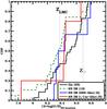 |
Fig. 15 CDFs of the metallicity at the SN location for SN IM subtypes, mainly based on NCR values. |
H14 presented a comprehensive study of the association with SF regions for CSI transients, where they introduced a subclassification of the SN IMs: SN 2008S-like and η Carinae-like. The first ones (SNe 2008S, 1999bw, 2001ac, 2002bu, 2010dn, 2008-OT) do not show any association with bright H ii regions (NCR = 0) and are often enshrouded in dusty environments. The second category (SNe 1954J, 1961V, 1997bs, 2002kg and V1) are associated with SF regions (NCR > 0). Also, because of the weak association with H ii regions, the first class of SN IMs may be related to 8–10 M⊙ super-AGBs (Prieto et al. 2008b; Botticella et al. 2009; Pumo et al. 2009; Wanajo et al. 2009; Kochanek 2011; Szczygieł et al. 2012) rather than to more massive LBV progenitors (see, however, Smith & Tombleson 2015), which are more likely to produce η Carinae-like IMs. When comparing the metallicity distributions of these two populations, we do not find any statistically significant difference (see Fig. 15). However, the numbers are small and the uncertainties are large. The same is true for SNe IIn and Ibn. If we plot the SN IM properties from Smith et al. (2011a) (see previous section) against the NCR values from H14, we do not find any clear trends or correlations. Furthermore, the NCR does not exhibit any clear trends with peak absolute magnitudes, mass-loss rate, or CSM/wind velocity in SNe IIn. In the last column of Table 4, we list all the available NCR values from H14. We note that Crowther (2013) concluded that the observed association between CC SNe and H ii regions only provides weak constraints upon the progenitor masses.
8. Discussion
8.1. Implications for the SN IIn progenitor scenario
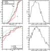 |
Fig. 16 Top left panel: metallicity CDFs of SNe IIn, SN IMs, SNe IIP, and of a simulated SN progenitor population constructed of SN IM/LBVs and SN IIP/RSGs, which fit the observed SN IIn metallicity CDF. Top right panel: p-value of the K-S test between the metallicity distributions of SNe IIn and the simulated progenitor population as a function of the fraction of LBVs in the simulated progenitor population. Bottom left panel: NCR CDFs of SNe IIn, SN IMs, SNe IIP, and of a simulated SN progenitor population made of SN IM/LBVs and SN IIP/RSGs, which fit the observed SN IIn NCR CDF. Data from H14 and Anderson et al. (2012). Bottom right panel: p-value of the K-S test between the NCR distributions of SNe IIn and the simulated progenitor population as a function of the fraction of SN IM/LBVs in the simulated progenitor population. |
As described in the introduction, there are several indications that LBVs, which likely produce SN IMs, are also progenitors of at least a fraction of SNe IIn. On the other hand, the large variety of SNe IIn may suggest the existence of multiple precursor channels. The latter is also consistent with our result for the different metallicity distributions of SNe IIn and SN IMs. Since we know that at least some SNe IIn are produced by the terminal explosion of LBVs (see, e.g., Pastorello et al. 2007; Gal-Yam et al. 2007; Ofek et al. 2014), and assuming that most of the SN IMs are produced by LBVs, then the metallicity distribution of SNe IIn can be considered to be a combination of the metallicity distribution of SN IMs with that of one or more alternative progenitor populations. These other progenitors must have higher metallicity than that of SN IMs, which would explain why SNe IIn are found at higher metallicity compared to SN IMs.
RSG stars with superwinds like VY Canis Majoris have been invoked as possible progenitors of some SNe IIn (e.g., Fransson et al. 2002; Smith et al. 2009a). If all the SNe IIn that are not produced by LBVs are actually produced by RSGs, and if we assume that the metallicity distribution of SNe IIP (which do have RSG progenitors, Smartt 2009) and that of RSGs producing SNe IIn are the same, then we can combine the metallicity distributions of SN IMs and SNe IIP to reproduce the observed metallicity distribution of SNe IIn. This exercise allows us to roughly estimate what fractions of LBVs and RSGs are precursors of SNe IIn, in a simple two-progenitor population scenario. This is done by maximizing the p-value of the K-S test between the SN IIn metallicity distribution and that of the combined distributions of SN IMs/LBVs+SNe IIP/RSGs. To produce combined metallicity distributions of SN IMs/LBVs and SNe IIP/RSGs, we linearly interpolate their observed CDFs (which are marked with a green dashed line and a red solid line in the top left panel of Fig. 16) varying the number of objects in the two samples, while always keeping a total of 35 events, which is the number of SNe IIn that we have in the metallicity CDF (solid black line in the top-left panel of Fig. 16). This is done to produce a meaningful comparison to the sample of SNe IIn. The two extreme cases are obtained when the combined distribution contains only SN IMs/LBVs or only SNe IIP/RSGs. In between, we obtain 33 different distributions with mixed fractions of SNe IIP/RSGs and SN IMs/LBVs. We then performed the K-S test between all these distributions and that for SNe IIn, and plot the resulting p-values as a function of the SN IMs/LBV fraction in the top right panel of Fig. 16. It is evident that the p-value reaches its maximum between ~28% and ~48% of SN IMs/LBVs as SN IIn progenitors, with the rest being formed by SN IIP/RSGs. This range would change to 20–35% if we exclude the hosts where we adopted the gradient from P04. The CDF formed by 40% of SN IMs and 60% of SNe IIP/RSGs is shown with a dashed line in the top left panel of Fig. 16, and it is a good match to the distribution of SNe IIn. Among SNe IIn, those resembling SN 1998S show a metallicity distribution similar to those of SNe IIP and IIL, suggesting that this SN IIn subclass might preferentially arise from RSGs rather than from LBVs. On the contrary, 1988Z-like SNe show a metallicity distribution consistent with that of the SN IMs, indicating a LBV origin.
By using data from H14 and Anderson et al. (2012), a similar exercise was repeated with the NCR distributions for SNe IIn, SN IMs, and SNe IIP. We found (see the bottom panels of Fig. 16) that the SN IIn NCR distribution can be reproduced with high statistical significance by a simulated population of SN IMs (from LBVs, ~40%) and SNe IIP (from RSGs, ~60%), identical to what was found when comparing the metallicity distributions. Ofek et al. (2014) estimate that ~50% of SNe IIn show outbursts only a few years before collapse, which is similar to our fraction of SN IMs/LBVs. This might imply that most LBV progenitors of SNe IIn display outbursts just before collapse. Indeed it has been found by Moriya et al. (2014) that SN IIn progenitors suffer enhanced mass loss as they get closer to collapse.
In reality, the scenario is likely more complicated, especially if we consider that some SN IMs, i.e., the SN 2008S-like events, are likely produced by super-AGB stars, and not by LBV eruptions. However, the metallicity distribution of SN IMs like SN 2008S is very similar to that of SN IMs like η Carinae (which are likely produced by LBV eruptions). From this perspective, we can consider the estimated 40% of LBV progenitors as an upper limit. It is more realistic to think that of this 40% some SN IIn have for instance super-AGB stars as precursors. SNe IIn-P (1994W-like events), which indeed show a metallicity distribution similar to SN IMs (see Fig. 10, left hand panel), might be the result of EC-SNe from super-AGB stars.
If we look at SN rates, SN II (IIP and IIL) and SNe IIn form ~55% and ~9% of the CC SNe (Smith et al. 2011b), respectively. In our simplified two-progenitor population scenario, ~60% of the SNe IIn comes from RSGs with large mass-loss rates (similar to the massive hypergiant VY Canis Majoris). If we assume a Salpeter initial mass function and single stars as progenitors, to reproduce the ratio between SNe IIn from RSGs and SNe II (~10%) would require that RSG stars with initial mass between 8 and 20 M⊙ produce SNe IIP/L and massive RSG stars with initial mass between 20 and 25 M⊙ produce SNe IIn. These ranges are reasonable, but they do not account for binary systems, which might be important to explain the progenitors of SNe IIn (Smith & Tombleson 2015) and other CC SNe.
There are potential biases in the samples of SNe IIn and SN IMs, which might affect the comparison between their metallicity distributions. Most of the SNe in our samples were discovered by galaxy-targeted surveys, with the exceptions of a few SDSS (Sloan Digital Sky Survey) II SN survey and PTF SNe. Targeted surveys often pitch larger galaxies with more metal rich distributions that the non targeted surveys (see, e.g., Sanders et al. 2012), so both of these distributions are likely biased in that direction.
The SNe IIn are also located at larger redshifts than the SN IMs. The latter are more difficult to discover at large distances given that they are typically ~4 mag fainter than SNe IIn. For the redshifts in this investigation, however, there is no metallicity evolution expected (see, e.g., Savaglio 2006). There is also no clear correlation between the SN IIn luminosity and their host metallicity, with the brighter SNe IIn (more likely to be discovered at larger distances) showing similar host metallicity to the fainter SNe IIn.
As most SNe IIn are selected based on the availability of literature data, it could be that the SN IIn sample is biased toward peculiar objects, which are more often discussed in the literature as compared to the “normal” SNe. It is, however, unclear if and how this selection would affect the observed metallicity distribution.
An alternative interpretation of the difference between the metallicity distribution of SN IMs and SNe IIn might be the following. If we instead assume that all the SNe IIn are actually produced by LBV stars, then the SN IMs are preferentially produced by the LBV at low metallicity, whereas at relatively high metallicity LBV would not produce giant outbursts but only exhibit, e.g., S-Doradus variability. However, we do know that large eruptions like η Car and other LBVs are found in both the MW and other nearby metal-rich galaxies (e.g., M 31, M 81, M 101), as well as in nearby metal-poor galaxies, such as NGC 2366 and the SMC (see Weis 2006, for a list of LBVs and their metallicities). We therefore do not favor this explanation for the lower metallicity of SN IMs as compared to that of SNe IIn.
8.2. Implications for the mass-loss mechanism
The large mass-loss rates derived for SN IIn progenitors and observed in SN IMs are not explicable solely in terms of steady, metal line-driven winds (Smith 2014). This mechanism cannot reproduce Ṁ> 10-4M⊙ yr-1, which we typically deduce for these transients. Eruptive mechanisms must play an important role.
The relation between metallicity and outbursts has not yet been clarified, but here we present a number of related observational results. We also need to consider that, via steady line-driven winds, the metallicity might have an effect on the appearance of CSI transients anyway, as they act for the entire life of their progenitors.
Despite the large spread, in SNe IIn it is possible to see that higher mass-loss rates and faster CSM velocities correlate with higher metallicity at the SN location (Fig. 12). Note that most of the mass-loss rate estimates used assume steady winds as well as shock velocities derived from the width of the broad component of Hα, even if the progenitor winds may in fact not be steady (Dwarkadas 2011), and the broad component of the emission lines can be due to Thomson scattering in a dense CSM (Chugai et al. 2002).
The bottom panel of Fig. 14 shows that in SN IMs, a higher metallicity tends to prompt relatively brighter outbursts in the optical. ΔM might be produced by an actual variation in the bolometric luminosity of the SN IM or be the effect of a temperature variation at almost constant bolometric luminosity as is observed for “S Doradus” LBVs (e.g., Humphreys & Davidson 1994, Vink 2011). These LBVs present temperatures of several 104 K in the quiescent state, and then become F-type stars (with temperatures of 8–9 × 10³ K) during the outburst. In this case, at larger metallicity we would have found the SN IMs whose photospheric temperatures suffered the stronger cooling during the outburst, i.e., the SN IMs whose progenitors had the higher temperatures before the outburst. More bolometric information on our SN IMs are necessary to draw further conclusions.
The fact that we found relatively brighter outbursts at larger metallicity might fit with the mass-loss bistability jump scenario discussed by Vink (2011) for LBVs. When a LBV becomes cooler than 2.5 × 10⁴ K, the Fe recombines from Fe iv to Fe iii, enhancing the opacity and thus the mass loss. LBVs are likely to cross the bistability temperature threshold several times during their lives, inducing variable mass loss. Obviously, large metallicities would favor this mass-loss enhancement and hence the luminosity in the eruptive phase.
Figure 14 (central panel) shows that progenitors of SN IM outbursts at lower metallicity tend to have higher optical luminosity. If we assume similar temperatures for the SN IM progenitors, this would mean that those with higher bolometric luminosity tend to be more metal poor. However, if we instead assume that they have similar bolometric luminosities, the brighter the progenitor in the optical, the lower its temperature would be. Therefore a possible implication of this result is that the cooler progenitors of SN IMs tend to have lower metallicities. Again, more data are needed to establish the bolometric and color properties of SN IMs.
The fact that at higher metallicity SN IMs show larger ΔM but their progenitor show lower absolute magnitudes could also be explained if we take into account the presence of dust in SN IMs. A larger metallicity would favor larger mass loss and thus stronger CSM interaction (and larger ΔM), but at the same time more dust would surround the star and thus the progenitor would suffer from larger extinction. However, there are SN IMs with large ΔM both with (SN 2008S, SN 2010dn, OT2008) and without (SNe 1997bs and 2003gm) dust emission (Thompson et al. 2009).
9. Conclusions
We summarize our main findings as follows:
-
SNe IIn are located at higher metallicities thanSN IMs, and this difference is statisticallysignificant.
-
The locations of SNe IIn-L (1998S-like) exhibit the highest metallicities among SNe IIn. Their metallicity distribution is similar to those of SNe IIL and IIP (produced by RSG progenitors). On the other hand, long-lasting SNe IIn (1988Z-like) are typically metal-poorer and exhibit a metallicity distribution similar to that of SN IMs (that may be produced by LBV progenitors).
-
The metallicity distribution of SNe IIn can be interpreted as a combination of the metallicity distributions of SN IMs and SNe IIP, which might be similar to the metallicity distributions of LBVs and RSG stars, respectively. The same is true for the NCR distribution of SNe IIn. These results on the metallicity and NCR distributions are consistent with a scenario in which SNe IIn have both LBV (~40%) and RSG (~60%) progenitors. If we also consider the possibility that some SN IMs come from super-AGB stars, then the estimated ~40% fraction of LBV progenitors might be considered as an upper limit.
-
We do not find a significant difference in the metallicity distributions of CSI SNe with and without dust emission in the MIR, but rather a difference in the distributions of the peak absolute magnitude, with the dust-rich SNe being brighter.
-
Above Ṁ ~ 10-3M⊙ yr-1, SNe IIn located at higher metallicities tend to show larger mass-loss rates. There are also indications of larger CSM/wind velocities for SNe IIn at higher metallicity.
-
There are hints that at higher(lower) metallicity the difference in optical magnitudes between the SN IM progenitor and its outburst’s peak tend to be larger(smaller) and SN IM progenitors tend to have lower(higher) optical luminosity.
Online material
Sample and basic data of 63 (38 SNe IIn, 6 SNe Ibn, 1 SN Ia-CSM, 18 SN IMs) CSI SN host galaxies.
Log of the photometric and spectroscopic observations at the Nordic Optical Telescope with ALFOSC.
Deprojected and normalized distance from the host center and line ratios for the H ii regions with observed spectrum.
Apparent (u/U,B,V,R/r/unf.,I/i) peak magnitudes, galactic and host extinction for the SNe IIn, Ibn, and Ia-CSM of our sample.
Absolute (U/u,B,V,R/r/unf.,I/i) peak magnitudes for the SNe IIn, Ibn, and Ia-CSM of our sample.
Wind velocity and mass-loss rate for a subsample of CSI SNe (IIn, Ibn, Ia-CSM).
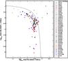 |
Fig. 4 BPT diagram for each H ii region that we spectroscopically observed. Above the dashed line (Kauffmann et al. 2003, see Sect. 4) the line fluxes are AGN contaminated and we rejected those spectra from our metallicity study. Most of the spectra fall in the star-forming part of the BPT diagram, below the dashed line. The symbols marked with black edges indicate that the ratio between [O iiiλ5007] and Hβ is an upper limit. All the line ratios are reported in Table 3. |
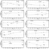 |
Fig. 5 Metallicity gradients of ten SN IIn host galaxies observed with the NOT+ALFOSC. Symbols and lines as in the bottom panel of Fig. 2. Black open squares with arrows correspond to upper limits. The gradients of the hosts of SNe 2006jd and 2005ip are not shown, as we could not measure the flux from bright H ii regions. Instead, we used literature data. For the host of SN 1995N, whose gradient is not shown, we only have one measurement and we did not assume any gradient, as it is an irregular and interacting galaxy. |
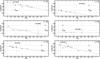 |
Fig. 6 Metallicity gradients of five SN Ibn and one SN Ia-CSM host galaxies observed with the NOT+ALFOSC. Symbols and lines as in the bottom panel of Fig. 2. |
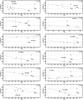 |
Fig. 7 Metallicity gradients of twelve SN IM host galaxies observed with the NOT+ALFOSC. Symbols and lines as in the bottom panel of Fig. 2. We label the gradient “P04" when we use the one measured by Pilyugin et al. (2004), and “⟨P04⟩" when we assumed the average P04 gradient. The data of the hosts of V1 and OT2005 are not shown as we do not determine or adopt a gradient for them, but we only measured the metallicity of one H ii region close the SN location. |
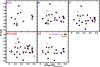 |
Fig. 11 Absolute peak magnitudes for SNe IIn and Ibn against the metallicity at the SN position. Triangles are upper limits. |
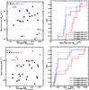 |
Fig. 12 Top left panel: mass-loss rates of SNe IIn versus local metallicity measurements. Triangles are upper limits. Above 10-3M⊙ yr-1, the mass-loss rates appear to be higher at higher metallicity. The power-law (PL) dependence on metallicity (α = 0.69 e.g., Vink 2011) of the line-driven mass-loss rates is shown with a black segment and is consistent with the data. SNe IIn-L (98S-like) typically show lower mass-loss rates than long-lasting SN IIn (88Z-like). Top right panel: mass-loss rate CDFs for metal-poor and metal-rich SNe IIn, shown to better highlight that at higher metallicities the mass-loss rates tend to be higher. Two different metallicity cuts are shown, at log(O/H) + 12 = 8.3 and 8.5. Bottom left panel: wind velocities of SNe IIn and SNe Ibn versus local metallicities. Triangles are upper limits. The PL dependence on metallicity (α= 0.12 (e.g., Kudritzki 2002) of the line-driven wind velocities rates is shown with a black segment, and is consistent with the data. SNe IIn-L (98S-like) typically show higher wind velocities than long-lasting SN IIn (88Z-like). Bottom right panel: wind-velocity CDFs, for metal-poor and metal-rich SNe IIn, shown to better highlight that at higher metallicities the wind velocities tend to be slightly higher. Two different metallicity cuts are shown, at log(O/H) + 12 = 8.3 and 8.5. |
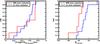 |
Fig. 13 Left-hand panel: metallicity CDFs for CSI SNe showing and not showing MIR dust emission at late epochs (Fox et al. 2011). These CDFs do not show any statistically significant difference. Right-hand panel: CDFs of the peak absolute r/R/unf. band magnitudes for the same CSI SNe showing and not showing MIR dust emission at late epochs. These CDFs show that SNe with MIR dust emission tend to be brighter at peak. |
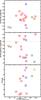 |
Fig. 14 Top panel: SN IM peak absolute magnitudes (from Smith et al. 2011a) versus local metallicity. Central panel: absolute magnitude of SN IM progenitors (from Smith et al. 2011a) versus local metallicities. Triangles are lower limits. With the exception of SN 1961V and of those events where we have limits poorer than −12 mag, at lower metallicity the luminosity seems to be higher. Bottom panel: difference between each peak outburst and the corresponding progenitor magnitude versus metallicity is shown. Triangles are lower limits. The data suggest larger ΔM at larger metallicity. Red corresponds to R/unf. bands, blue to B band, green to V band, magenta to I band, brown to NIR, orange to R/V. |
Nasa Extragalactic Database, http://ned.ipac.caltech.edu/
Acknowledgments
We gratefully acknowledge the support from the Knut and Alice Wallenberg Foundation. A. Pastorello is partially supported by the PRIN-INAF 2014 with the project “transient Universe: unveiling new types of stellar explosions with PESSTO”. M. D. Stritzinger gratefully acknowledges generous support provided by the Danish Agency for Science and Technology and Innovation realized through a Sapere Aude Level 2 grant. The Oskar Klein Centre is funded by the Swedish Research Council. The Nordic Optical Telescope is operated by the Nordic Optical Telescope Scientific Association at the Observatorio del Roque de los Muchachos, La Palma, Spain, of the Instituto de Astrofisica de Canarias. This research has made use of the NASA/IPAC Extragalactic Database (NED), which is operated by the Jet Propulsion Laboratory, California Institute of Technology, under contract with the National Aeronautics and Space Administration.
References
- Aldering, G., Antilogus, P., Bailey, S., et al. 2006, ApJ, 650, 510 [NASA ADS] [CrossRef] [Google Scholar]
- Anderson, J. P., & James, P. A. 2008, MNRAS, 390, 1527 [NASA ADS] [Google Scholar]
- Anderson, J. P., Covarrubias, R. A., James, P. A., Hamuy, M., & Habergham, S. M. 2010, MNRAS, 407, 2660 [NASA ADS] [CrossRef] [Google Scholar]
- Anderson, J. P., Habergham, S. M., James, P. A., & Hamuy, M. 2012, MNRAS, 424, 1372 [NASA ADS] [CrossRef] [Google Scholar]
- Anderson, J. P., James, P. A., Habergham, S. M., Galbany, L., & Kuncarayakti, H. 2015, PASA, 32, e019 [NASA ADS] [CrossRef] [Google Scholar]
- Anupama, G. C., Sivarani, T., & Pandey, G. 2001, A&A, 367, 506 [NASA ADS] [CrossRef] [EDP Sciences] [Google Scholar]
- Anupama, G. C., Sahu, D. K., Gurugubelli, U. K., et al. 2009, MNRAS, 392, 894 [NASA ADS] [CrossRef] [Google Scholar]
- Aretxaga, I., Benetti, S., Terlevich, R. J., et al. 1999, MNRAS, 309, 343 [NASA ADS] [CrossRef] [Google Scholar]
- Asplund, M., Grevesse, N., Sauval, A. J., & Scott, P. 2009, ARA&A, 47, 481 [NASA ADS] [CrossRef] [Google Scholar]
- Baldwin, J. A., Phillips, M. M., & Terlevich, R. 1981, PASP, 93, 5 [NASA ADS] [CrossRef] [EDP Sciences] [Google Scholar]
- Belfiore, F., Maiolino, R., Bundy, K., et al. 2015, MNRAS, 449, 867 [NASA ADS] [CrossRef] [Google Scholar]
- Benetti, S., Cappellaro, E., Danziger, I. J., et al. 1998, MNRAS, 294, 448 [NASA ADS] [CrossRef] [Google Scholar]
- Benetti, S., Turatto, M., Cappellaro, E., Danziger, I. J., & Mazzali, P. A. 1999, MNRAS, 305, 811 [NASA ADS] [CrossRef] [Google Scholar]
- Benetti, S., Cappellaro, E., Turatto, M., et al. 2006, ApJ, 653, L129 [NASA ADS] [CrossRef] [MathSciNet] [Google Scholar]
- Botticella, M. T., Pastorello, A., Smartt, S. J., et al. 2009, MNRAS, 398, 1041 [NASA ADS] [CrossRef] [Google Scholar]
- Bruzual, G., & Charlot, S. 2003, MNRAS, 344, 1000 [NASA ADS] [CrossRef] [Google Scholar]
- Chevalier, R. A., & Fransson, C. 1994, ApJ, 420, 268 [NASA ADS] [CrossRef] [Google Scholar]
- Chugai, N. N. 1991, MNRAS, 250, 513 [NASA ADS] [CrossRef] [Google Scholar]
- Chugai, N. N., & Danziger, I. J. 1994, MNRAS, 268, 173 [NASA ADS] [Google Scholar]
- Chugai, N. N., & Danziger, I. J. 2003, Astron. Lett. 29, 649 [NASA ADS] [CrossRef] [Google Scholar]
- Chugai, N. N., & Utrobin, V. P. 2008, Astron. Lett., 34, 589 [NASA ADS] [CrossRef] [Google Scholar]
- Chugai, N. N., Blinnikov, S. I., Fassia, A., et al. 2002, MNRAS, 330, 473 [NASA ADS] [CrossRef] [Google Scholar]
- Chugai, N. N., Blinnikov, S. I., Cumming, R. J., et al. 2004, MNRAS, 352, 1213 [NASA ADS] [CrossRef] [Google Scholar]
- Cid Fernandes, R., Mateus, A., Sodré, L., Stasińska, G., & Gomes, J. M. 2005, MNRAS, 358, 363 [NASA ADS] [CrossRef] [Google Scholar]
- Clark, J. S., Crowther, P. A., Larionov, V. M., et al. 2009, A&A, 507, 1555 [NASA ADS] [CrossRef] [EDP Sciences] [Google Scholar]
- Crowther, P. A. 2013, MNRAS, 428, 1927 [NASA ADS] [CrossRef] [Google Scholar]
- de Vaucouleurs, G., de Vaucouleurs, A., Corwin, H. G., Jr., et al. 1991, Third Reference Catalogue of Bright Galaxies [Google Scholar]
- Dessart, L., Hillier, D. J., Gezari, S., Basa, S., & Matheson, T. 2009, MNRAS, 394, 21 [NASA ADS] [CrossRef] [Google Scholar]
- Di Carlo, E., Massi, F., Valentini, G., et al. 2002, ApJ, 573, 144 [NASA ADS] [CrossRef] [Google Scholar]
- Dilday, B., Howell, D. A., Cenko, S. B., et al. 2012, Science, 337, 942 [NASA ADS] [CrossRef] [Google Scholar]
- Dwarkadas, V. V. 2011, MNRAS, 412, 1639 [NASA ADS] [CrossRef] [Google Scholar]
- Fassia, A., Meikle, W. P. S., Vacca, W. D., et al. 2000, MNRAS, 318, 1093 [NASA ADS] [CrossRef] [Google Scholar]
- Fassia, A., Meikle, W. P. S., Chugai, N., et al. 2001, MNRAS, 325, 907 [NASA ADS] [CrossRef] [Google Scholar]
- Foley, R. J., Smith, N., Ganeshalingam, M., et al. 2007, ApJ, 657, L105 [NASA ADS] [CrossRef] [Google Scholar]
- Foley, R. J., Berger, E., Fox, O., et al. 2011, ApJ, 732, 32 [NASA ADS] [CrossRef] [Google Scholar]
- Fox, O., Skrutskie, M. F., Chevalier, R. A., et al. 2009, ApJ, 691, 650 [NASA ADS] [CrossRef] [Google Scholar]
- Fox, O. D., Chevalier, R. A., Skrutskie, M. F., et al. 2011, ApJ, 741, 7 [NASA ADS] [CrossRef] [Google Scholar]
- Fox, O. D., Silverman, J. M., Filippenko, A. V., et al. 2015, MNRAS, 447, 772 [NASA ADS] [CrossRef] [Google Scholar]
- Fransson, C., Chevalier, R. A., Filippenko, A. V., et al. 2002, ApJ, 572, 350 [NASA ADS] [CrossRef] [Google Scholar]
- Fransson, C., Challis, P. M., Chevalier, R. A., et al. 2005, ApJ, 622, 991 [NASA ADS] [CrossRef] [Google Scholar]
- Fransson, C., Ergon, M., Challis, P. J., et al. 2014, ApJ, 797, 118 [NASA ADS] [CrossRef] [Google Scholar]
- Fraser, M., Inserra, C., Jerkstrand, A., et al. 2013, MNRAS, 433, 1312 [NASA ADS] [CrossRef] [Google Scholar]
- Friedman, A., Li, W. D., & Puckett, T. 1999, IAU Circ., 7316, 2 [NASA ADS] [Google Scholar]
- Galbany, L., Stanishev, V., Mourão, A. M., et al. 2014, A&A, 572, A38 [NASA ADS] [CrossRef] [EDP Sciences] [Google Scholar]
- Gal-Yam, A. 2012, Science, 337, 927 [NASA ADS] [CrossRef] [PubMed] [Google Scholar]
- Gal-Yam, A., & Leonard, D. C. 2009, Nature, 458, 865 [NASA ADS] [CrossRef] [PubMed] [Google Scholar]
- Gal-Yam, A., Leonard, D. C., Fox, D. B., et al. 2007, ApJ, 656, 372 [NASA ADS] [CrossRef] [Google Scholar]
- Gorbikov, E., Gal-Yam, A., Ofek, E. O., et al. 2014, MNRAS, 443, 671 [NASA ADS] [CrossRef] [Google Scholar]
- Habergham, S. M., Anderson, J. P., James, P. A., & Lyman, J. D. 2014, MNRAS, 441, 2230 [H14] [NASA ADS] [CrossRef] [Google Scholar]
- Hagen, H.-J., Engels, D., & Reimers, D. 1997, A&A, 324, L29 [NASA ADS] [Google Scholar]
- Hakobyan, A. A., Adibekyan, V. Z., Aramyan, L. S., et al. 2012, A&A, 544, A81 [NASA ADS] [CrossRef] [EDP Sciences] [Google Scholar]
- Hakobyan, A. A., Mamon, G. A., Petrosian, A. R., Kunth, D., & Turatto, M. 2009, A&A, 508, 1259 [NASA ADS] [CrossRef] [EDP Sciences] [Google Scholar]
- Hamuy, M., Phillips, M. M., Suntzeff, N. B., et al. 2003, Nature, 424, 651 [NASA ADS] [CrossRef] [Google Scholar]
- Humphreys, R. M., & Davidson, K. 1994, PASP, 106, 1025 [NASA ADS] [CrossRef] [Google Scholar]
- Humphreys, R. M., Davidson, K., Jones, T. J., et al. 2012, ApJ, 760, 93 [NASA ADS] [CrossRef] [Google Scholar]
- Inserra, C., Smartt, S. J., Scalzo, R., et al. 2014, MNRAS, 437, L51 [NASA ADS] [CrossRef] [Google Scholar]
- Izotov, Y. I., Stasińska, G., Meynet, G., Guseva, N. G., & Thuan, T. X. 2006, A&A, 448, 955 [NASA ADS] [CrossRef] [EDP Sciences] [Google Scholar]
- Kankare, E., Ergon, M., Bufano, F., et al. 2012, MNRAS, 424, 855 [NASA ADS] [CrossRef] [Google Scholar]
- Kauffmann, G., Heckman, T. M., Tremonti, C., et al. 2003, MNRAS, 346, 1055 [Google Scholar]
- Kehrig, C., Monreal-Ibero, A., Papaderos, P., et al. 2012, A&A, 540, A11 [NASA ADS] [CrossRef] [EDP Sciences] [Google Scholar]
- Kelly, P. L., & Kirshner, R. P. 2012, ApJ, 759, 107 [NASA ADS] [CrossRef] [Google Scholar]
- Kewley, L. J., & Ellison, S. L. 2008, ApJ, 681, 1183 [NASA ADS] [CrossRef] [Google Scholar]
- Kewley, L. J., Dopita, M. A., Sutherland, R. S., Heisler, C. A., & Trevena, J. 2001, ApJ, 556, 121 [Google Scholar]
- Kelly, P. L., Filippenko, A. V., Modjaz, M., & Kocevski, D. 2014, ApJ, 789, 23 [NASA ADS] [CrossRef] [Google Scholar]
- Kiewe, M., Gal-Yam, A., Arcavi, I., et al. 2012, ApJ, 744, 10 [NASA ADS] [CrossRef] [Google Scholar]
- Kochanek, C. S. 2011, ApJ, 741, 37 [NASA ADS] [CrossRef] [Google Scholar]
- Kochanek, C. S. 2014, MNRAS, 444, 2043 [NASA ADS] [CrossRef] [Google Scholar]
- Kozłowski, S., Kochanek, C. S., Stern, D., et al. 2010, ApJ, 722, 1624 [NASA ADS] [CrossRef] [Google Scholar]
- Kudritzki, R. P. 2002, ApJ, 577, 389 [NASA ADS] [CrossRef] [Google Scholar]
- Kudritzki, R.-P., & Puls, J. 2000, ARA&A, 38, 613 [NASA ADS] [CrossRef] [Google Scholar]
- Kuncarayakti, H., Doi, M., Aldering, G., et al. 2013a, AJ, 146, 30 [NASA ADS] [CrossRef] [Google Scholar]
- Kuncarayakti, H., Doi, M., Aldering, G., et al. 2013b, AJ, 146, 31 [NASA ADS] [CrossRef] [Google Scholar]
- James, P. A., & Anderson, J. P. 2006, A&A, 453, 57 [NASA ADS] [CrossRef] [EDP Sciences] [Google Scholar]
- Jones, D. H., Read, M. A., Saunders, W., et al. 2009, MNRAS, 399, 683 [NASA ADS] [CrossRef] [Google Scholar]
- Lee, E., & Li, W. 2006, Central Bureau Electronic Telegrams, 412, 1 [NASA ADS] [Google Scholar]
- Leloudas, G., Gallazzi, A., Sollerman, J., et al. 2011, A&A, 530, A95 [NASA ADS] [CrossRef] [EDP Sciences] [Google Scholar]
- Leloudas, G., Schulze, S., Kruehler, T., et al. 2015a, MNRAS, 449, 917 [NASA ADS] [CrossRef] [Google Scholar]
- Leloudas, G., Hsiao, E. Y., Johansson, J., et al. 2015b, A&A, 574, A61 [NASA ADS] [CrossRef] [EDP Sciences] [Google Scholar]
- Liu, Q.-Z., Hu, J.-Y., Hang, H.-R., et al. 2000, A&AS, 144, 219 [NASA ADS] [CrossRef] [EDP Sciences] [Google Scholar]
- Lundqvist, P., & Fransson, C. 1988, A&A, 192, 221 [NASA ADS] [Google Scholar]
- Mackey, J., Mohamed, S., Gvaramadze, V. V., et al. 2014, Nature, 512, 282 [NASA ADS] [CrossRef] [Google Scholar]
- Margutti, R., Milisavljevic, D., Soderberg, A. M., et al. 2014, ApJ, 780, 21 [NASA ADS] [CrossRef] [Google Scholar]
- Marino, R. A., Rosales-Ortega, F. F., Sánchez, S. F., et al. 2013, A&A, 559, A114 [NASA ADS] [CrossRef] [EDP Sciences] [Google Scholar]
- Matheson, T., Filippenko, A. V., Chornock, R., Leonard, D. C., & Li, W. 2000, AJ, 119, 2303 [NASA ADS] [CrossRef] [Google Scholar]
- Mauerhan, J. C., Smith, N., Filippenko, A. V., et al. 2013a, MNRAS, 430, 1801 [NASA ADS] [CrossRef] [Google Scholar]
- Mauerhan, J. C., Smith, N., Silverman, J. M., et al. 2013b, MNRAS, 431, 2599 [NASA ADS] [CrossRef] [Google Scholar]
- Maund, J. R., Smartt, S. J., Kudritzki, R.-P., et al. 2006, MNRAS, 369, 390 [NASA ADS] [CrossRef] [Google Scholar]
- Modjaz, M., Kewley, L., Bloom, J. S., et al. 2011, ApJ, 731, L4 [NASA ADS] [CrossRef] [Google Scholar]
- Mollá, M., Vílchez, J. M., Gavilán, M., & Díaz, A. I. 2006, MNRAS, 372, 1069 [NASA ADS] [CrossRef] [Google Scholar]
- Moriya, T. J., & Maeda, K. 2014, ApJ, 790, L16 [NASA ADS] [CrossRef] [Google Scholar]
- Moriya, T. J., Maeda, K., Taddia, F., et al. 2014, MNRAS, 439, 2917 [NASA ADS] [CrossRef] [Google Scholar]
- Nakano, S., & Kadota, K. 2008, Central Bureau Electronic Telegrams, 1194, 1 [NASA ADS] [Google Scholar]
- Niino, Y., Nagamine, K., & Zhang, B. 2015, MNRAS, 449, 2706 [NASA ADS] [CrossRef] [Google Scholar]
- Nomoto, K. 1984, ApJ, 277, 791 [NASA ADS] [CrossRef] [Google Scholar]
- Ofek, E. O., Sullivan, M., Shaviv, N. J., et al. 2014, ApJ, 789, 104 [NASA ADS] [CrossRef] [Google Scholar]
- Osterbrock, D. E., & Ferland, G. J. 2006, Astrophysics of gaseous nebulae and active galactic nuclei, 2nd. (Sausalito, CA: University Science Books) [Google Scholar]
- Pastorello, A., Turatto, M., Benetti, S., et al. 2002, MNRAS, 333, 27 [NASA ADS] [CrossRef] [Google Scholar]
- Pastorello, A., Aretxaga, I., Zampieri, L., Mucciarelli, P., & Benetti, S. 2005 [arXiv:astro-ph/0504116] [Google Scholar]
- Pastorello, A., Smartt, S. J., Mattila, S., et al. 2007, Nature, 447, 829 [NASA ADS] [CrossRef] [PubMed] [Google Scholar]
- Pastorello, A., Mattila, S., Zampieri, L., et al. 2008a, MNRAS, 389, 113 [NASA ADS] [CrossRef] [Google Scholar]
- Pastorello, A., Quimby, R. M., Smartt, S. J., et al. 2008b, MNRAS, 389, 131 [NASA ADS] [CrossRef] [Google Scholar]
- Pastorello, A., Botticella, M. T., Trundle, C., et al. 2010, MNRAS, 408, 181 [NASA ADS] [CrossRef] [Google Scholar]
- Pastorello, A., Cappellaro, E., Inserra, C., et al. 2013, ApJ, 767, 1 [NASA ADS] [CrossRef] [Google Scholar]
- Pastorello, A., Hadjiyska, E., Rabinowitz, D., et al. 2015a, MNRAS, 449, 1954 [NASA ADS] [CrossRef] [Google Scholar]
- Pastorello, A., Benetti, S., Brown, P. J., et al. 2015b, MNRAS, 449, 1921 [NASA ADS] [CrossRef] [Google Scholar]
- Pérez-Montero, E., & Contini, T. 2009, MNRAS, 398, 949 [NASA ADS] [CrossRef] [Google Scholar]
- Pettini, M., & Pagel, B. E. J. 2004, MNRAS, 348, L59 [NASA ADS] [CrossRef] [Google Scholar]
- Pilyugin, L. S., Vílchez, J. M., & Contini, T. 2004, A&A, 425, 849 [P04] [NASA ADS] [CrossRef] [EDP Sciences] [Google Scholar]
- Pumo, M. L., Turatto, M., Botticella, M. T., et al. 2009, ApJ, 705, L138 [NASA ADS] [CrossRef] [Google Scholar]
- Prieto, J. L., Stanek, K. Z., & Beacom, J. F. 2008a, ApJ, 673, 999 [NASA ADS] [CrossRef] [Google Scholar]
- Prieto, J. L., Kistler, M. D., Thompson, T. A., et al. 2008b, ApJ, 681, L9 [NASA ADS] [CrossRef] [Google Scholar]
- Prieto, J. L., Brimacombe, J., Drake, A. J., & Howerton, S. 2013, ApJ, 763, 27 [Google Scholar]
- Puckett, T., & Newton, J. 2002, IAU Circ., 7936, 1 [NASA ADS] [Google Scholar]
- Puckett, T., Kerns, B., & Toth, D. 2004, IAU Circ., 8261, 2 [NASA ADS] [Google Scholar]
- Quataert, E., & Shiode, J. 2012, MNRAS, 423, L92 [NASA ADS] [CrossRef] [Google Scholar]
- Qiu, Y. L., Hu, J. Y., & Bao Supernova, S. 2002, IAU Circ., 7786, 1 [NASA ADS] [Google Scholar]
- Quimby, R., & Mondol, P. 2006, Central Bureau Electronic Telegrams, 548, 1 [NASA ADS] [Google Scholar]
- Rest, A., Foley, R. J., Gezari, S., et al. 2011, ApJ, 729, 88 [NASA ADS] [CrossRef] [Google Scholar]
- Richmond, M. W., Treffers, R. R., van Dyk, S. D., et al. 1995, IAU Circ., 6123, 1 [NASA ADS] [Google Scholar]
- Riess, A. G., Macri, L., Casertano, S., et al. 2011, ApJ, 730, 119 [NASA ADS] [CrossRef] [Google Scholar]
- Roming, P. W. A., Pritchard, T. A., Prieto, J. L., et al. 2012, ApJ, 751, 92 [NASA ADS] [CrossRef] [Google Scholar]
- Russell, S. C., & Dopita, M. A. 1990, ApJS, 74, 93 [NASA ADS] [CrossRef] [Google Scholar]
- Salamanca, I., Cid-Fernandes, R., Tenorio-Tagle, G., et al. 1998, MNRAS, 300, L17 [NASA ADS] [CrossRef] [Google Scholar]
- Sánchez, S. F., Rosales-Ortega, F. F., Iglesias-Páramo, J., et al. 2014, A&A, 563, A49 [NASA ADS] [CrossRef] [EDP Sciences] [Google Scholar]
- Sanders, N. E., Soderberg, A. M., Levesque, E. M., et al. 2012, ApJ, 758, 132 [NASA ADS] [CrossRef] [Google Scholar]
- Sanders, N. E., Levesque, E. M., & Soderberg, A. M. 2013, ApJ, 775, 125 [NASA ADS] [CrossRef] [Google Scholar]
- Savaglio, S. 2006, New J. Phys., 8, 195 [NASA ADS] [CrossRef] [Google Scholar]
- Schlafly, E. F., & Finkbeiner, D. P. 2011, ApJ, 737, 103 [NASA ADS] [CrossRef] [Google Scholar]
- Schlegel, E. M. 1990, MNRAS, 244, 269 [NASA ADS] [Google Scholar]
- Silverman, J. M., Nugent, P. E., Gal-Yam, A., et al. 2013, ApJS, 207, 3 [NASA ADS] [CrossRef] [Google Scholar]
- Smartt, S. J. 2009, ARA&A, 47, 63 [NASA ADS] [CrossRef] [Google Scholar]
- Smith, N. 2014, ARA&A, 52, 487 [NASA ADS] [CrossRef] [MathSciNet] [Google Scholar]
- Smith, N., & Owocki, S. P. 2006, ApJ, 645, L45 [NASA ADS] [CrossRef] [Google Scholar]
- Smith, N., & Tombleson, R. 2015, MNRAS, 447, 598 [NASA ADS] [CrossRef] [Google Scholar]
- Smith, N., Li, W., Foley, R. J., et al. 2007, ApJ, 666, 1116 [NASA ADS] [CrossRef] [Google Scholar]
- Smith, N., Foley, R. J., & Filippenko, A. V. 2008a, ApJ, 680, 568 [NASA ADS] [CrossRef] [Google Scholar]
- Smith, N., Chornock, R., Li, W., et al. 2008b, ApJ, 686, 467 [NASA ADS] [CrossRef] [Google Scholar]
- Smith, N., Hinkle, K. H., & Ryde, N. 2009a, AJ, 137, 3558 [NASA ADS] [CrossRef] [Google Scholar]
- Smith, N., Silverman, J. M., Chornock, R., et al. 2009b, ApJ, 695, 1334 [NASA ADS] [CrossRef] [Google Scholar]
- Smith, N., Miller, A., Li, W., et al. 2010, AJ, 139, 1451 [NASA ADS] [CrossRef] [Google Scholar]
- Smith, N., Li, W., Silverman, J. M., Ganeshalingam, M., & Filippenko, A. V. 2011a, MNRAS, 415, 773 [NASA ADS] [CrossRef] [Google Scholar]
- Smith, N., Li, W., Filippenko, A. V., & Chornock, R. 2011b, MNRAS, 412, 1522 [NASA ADS] [CrossRef] [Google Scholar]
- Smith, N., Mauerhan, J. C., & Prieto, J. L. 2014, MNRAS, 438, 1191 [NASA ADS] [CrossRef] [Google Scholar]
- Smith, N., Mauerhan, J. C., Cenko, S. B., et al. 2015, MNRAS, 449, 1876 [NASA ADS] [CrossRef] [Google Scholar]
- Sollerman, J. 2002, New A Rev., 46, 493 [NASA ADS] [CrossRef] [Google Scholar]
- Sollerman, J., Cumming, R. J., & Lundqvist, P. 1998, ApJ, 493, 933 [NASA ADS] [CrossRef] [Google Scholar]
- Stanishev, V. 2007, Astron. Nachr., 328, 948 [NASA ADS] [CrossRef] [Google Scholar]
- Stathakis, R. A., & Sadler, E. M. 1991, MNRAS, 250, 786 [NASA ADS] [Google Scholar]
- Stoll, R., Prieto, J. L., Stanek, K. Z., et al. 2011, ApJ, 730, 34 [NASA ADS] [CrossRef] [Google Scholar]
- Stoll, R., Prieto, J. L., Stanek, K. Z., & Pogge, R. W. 2013, ApJ, 773, 12 [NASA ADS] [CrossRef] [Google Scholar]
- Stritzinger, M., Taddia, F., Fransson, C., et al. 2012, ApJ, 756, 173 [S12] [NASA ADS] [CrossRef] [Google Scholar]
- Swift, B., Foley, R., & Li, W. 2003, IAU Circ., 8243, 1 [NASA ADS] [Google Scholar]
- Swift, B., Burket, J., Pugh, H., et al. 2004, IAU Circ., 8271, 2 [NASA ADS] [Google Scholar]
- Szczygieł, D. M., Prieto, J. L., Kochanek, C. S., et al. 2012, ApJ, 750, 77 [NASA ADS] [CrossRef] [Google Scholar]
- Taddia, F., Stritzinger, M. D., Phillips, M. M., et al. 2012, A&A, 545, L7 [NASA ADS] [CrossRef] [EDP Sciences] [Google Scholar]
- Taddia, F., Stritzinger, M. D., Sollerman, J., et al. 2013a, A&A, 555, A10 [NASA ADS] [CrossRef] [EDP Sciences] [Google Scholar]
- Taddia, F., Sollerman, J., Razza, A., et al. 2013b, A&A, 558, A143 [NASA ADS] [CrossRef] [EDP Sciences] [Google Scholar]
- Tartaglia, L., Pastorello, A., Taubenberger, S., et al. 2015, MNRAS, 447, 117 [NASA ADS] [CrossRef] [Google Scholar]
- Thompson, T. A., Prieto, J. L., Stanek, K. Z., et al. 2009, ApJ, 705, 1364 [NASA ADS] [CrossRef] [Google Scholar]
- Tremonti, C. A., Heckman, T. M., Kauffmann, G., et al. 2004, ApJ, 613, 898 [NASA ADS] [CrossRef] [Google Scholar]
- Trundle, C., Pastorello, A., Benetti, S., et al. 2009, A&A, 504, 945 [NASA ADS] [CrossRef] [EDP Sciences] [Google Scholar]
- Tsvetkov, D. Y. 1995, Information Bulletin on Variable Stars, 4253, 1 [NASA ADS] [Google Scholar]
- Tsvetkov, D. Y., & Pavlyuk, N. N. 1997, Astron. Lett., 23, 26 [NASA ADS] [Google Scholar]
- Turatto, M., Cappellaro, E., Danziger, I. J., et al. 1993, MNRAS, 262, 128 [NASA ADS] [CrossRef] [Google Scholar]
- Thöne, C. C., Michałowski, M. J., Leloudas, G., et al. 2009, ApJ, 698, 1307 [NASA ADS] [CrossRef] [Google Scholar]
- Van Dyk, S. D., & Matheson, T. 2012, ApJ, 746, 179 [NASA ADS] [CrossRef] [Google Scholar]
- Vink, J. S. 2011, Ap&SS, 336, 163 [NASA ADS] [CrossRef] [Google Scholar]
- Wagner, R. M., Vrba, F. J., Henden, A. A., et al. 2004, PASP, 116, 326 [NASA ADS] [CrossRef] [Google Scholar]
- Wanajo, S., Nomoto, K., Janka, H.-T., Kitaura, F. S., Müller, B. 2009, ApJ, 695, 208 [NASA ADS] [CrossRef] [Google Scholar]
- Wegner, G., & Swanson, S. R. 1996, MNRAS, 278, 22 [NASA ADS] [CrossRef] [Google Scholar]
- Weis, K. 2006, Stellar Evolution at Low Metallicity: Mass Loss, Explosions, Cosmology, 353, 71 [Google Scholar]
- Zampieri, L., Mucciarelli, P., Pastorello, A., et al. 2005, MNRAS, 364, 1419 [NASA ADS] [CrossRef] [Google Scholar]
- Zhang, T., Wang, X., Wu, C., et al. 2012, AJ, 144, 131 [NASA ADS] [CrossRef] [Google Scholar]
All Tables
Metallicity estimates and normalized cumulative rank (NCR) pixel index for the sample of CSI transients.
Sample and basic data of 63 (38 SNe IIn, 6 SNe Ibn, 1 SN Ia-CSM, 18 SN IMs) CSI SN host galaxies.
Log of the photometric and spectroscopic observations at the Nordic Optical Telescope with ALFOSC.
Deprojected and normalized distance from the host center and line ratios for the H ii regions with observed spectrum.
Apparent (u/U,B,V,R/r/unf.,I/i) peak magnitudes, galactic and host extinction for the SNe IIn, Ibn, and Ia-CSM of our sample.
Absolute (U/u,B,V,R/r/unf.,I/i) peak magnitudes for the SNe IIn, Ibn, and Ia-CSM of our sample.
All Figures
|
Fig. 1 CSI SN classification scheme. Viable SN explosion mechanisms, the main elements in their spectra, their light curve properties (only for SN IIn subtypes), the degree of association (NCR) to H ii regions (only for SN IMs) and the possible progenitors are shown in correspondence with their CSI SN subtype. |
| In the text | |
|
Fig. 2 Top right panel: continuum-subtracted Hα image of UGC 4286, the host galaxy of SN 2010al. The 25th B-band magnitude elliptic contour is shown with a black solid line, along with the position of SN 2010al (marked by a red star) and the center of the galaxy (marked by a red circle). The slit position is shown, and a color code is used to present the N2 metallicity measurements at the position of each H ii region that we inspected. Top left panel: flux at the Hα wavelength along the slit, shown as a function of the distance from the SN location (marked by a dotted line, like the nucleus position). The N2 measurements are shown at the corresponding positions in the top subpanel. Bottom panel: metallicity gradient of UGC 4286. The linear fit on our measurements is shown with a solid line. The interpolated metallicity at the SN distance is marked with a red square and its uncertainty corresponds to the fit error. The error bar (±0.2) for our N2 measurements is shown aside. The positions of SN and nucleus are marked with vertical dotted lines. The solar metallicity (Asplund et al. 2009) and the LMC metallicity (Russell & Dopita 1990) are indicated with two horizontal dotted lines. |
| In the text | |
|
Fig. 3 Top panel: STARLIGHT stellar-population spectrum best fit to the continuum of the spectrum obtained at the center of the host galaxy of SN 2006aa. The difference between the observed spectrum and the best fit gives the pure emission-line spectrum. Bottom panel: the triple-Gaussian fit on the continuum-subtracted Hα and [N ii] lines of the bright H ii region at the center of the host galaxy of SN 2006aa. The observed fluxes are represented with black crosses, the best fit in red, the Hα component in blue, and the [N ii] components in green. |
| In the text | |
|
Fig. 8 Top left panel: cumulative distribution functions (CDFs) of the central metallicities for SN IIn, Ibn, and SN IM host galaxies. SN Ibn and SN IM hosts show slightly lower metallicities than SN IIn hosts. Top right panel: CDFs of the metallicity at the SN location for the same three classes. SN IMs and SNe Ibn are located in lower metallicity environments than those of SNe IIn. Bottom panels: CDFs of the host metallicity gradients and deprojected SN distances from the host center for SNe IIn, Ibn, and SN IMs. |
| In the text | |
|
Fig. 9 CDFs of the metallicity at the SN location for CSI transients and for other SN classes from the literature. We ordered the legend entries by mean metallicity. |
| In the text | |
|
Fig. 10 Left-hand panel: SN IIn light curves from the literature. Three main subclasses are identified (plus the SLSNe) based on the light curve shape. Long-lasting SNe IIn (1988Z-like; blue) show slow decline (~0.7 mag (100 days)-1) and sustained luminosity for ≳5 months. SN IIn-P (1994W-like; red) show a ~3–4 month plateau followed by a sharp drop, similar to what is observed in SNe IIP. SNe IIn-L (1998S or 1999el-like, depending on the spectral evolution; magenta) show a faster decline (~2.9 mag (100 days)-1). References for the light curve data and the extinction of SNe with measured metallicity can be found in Table 5. For SNe 1994aj, 1999el, 2005cl, 2006gy, 2006tf, and 2009kn, the references are Benetti et al. (1998), Di Carlo et al. (2002), Kiewe et al. (2012), Smith et al. (2007), Smith et al. (2008b), and Kankare et al. (2012), respectively. Right-hand panel: CDFs of the metallicity at the SN location for our CSI transients, including three SN IIn subclasses (1988Z-like, 1994W-like, 1998S-like). 1998S-like SNe are located at higher metallicity compared to the other subtypes. |
| In the text | |
|
Fig. 15 CDFs of the metallicity at the SN location for SN IM subtypes, mainly based on NCR values. |
| In the text | |
|
Fig. 16 Top left panel: metallicity CDFs of SNe IIn, SN IMs, SNe IIP, and of a simulated SN progenitor population constructed of SN IM/LBVs and SN IIP/RSGs, which fit the observed SN IIn metallicity CDF. Top right panel: p-value of the K-S test between the metallicity distributions of SNe IIn and the simulated progenitor population as a function of the fraction of LBVs in the simulated progenitor population. Bottom left panel: NCR CDFs of SNe IIn, SN IMs, SNe IIP, and of a simulated SN progenitor population made of SN IM/LBVs and SN IIP/RSGs, which fit the observed SN IIn NCR CDF. Data from H14 and Anderson et al. (2012). Bottom right panel: p-value of the K-S test between the NCR distributions of SNe IIn and the simulated progenitor population as a function of the fraction of SN IM/LBVs in the simulated progenitor population. |
| In the text | |
|
Fig. 4 BPT diagram for each H ii region that we spectroscopically observed. Above the dashed line (Kauffmann et al. 2003, see Sect. 4) the line fluxes are AGN contaminated and we rejected those spectra from our metallicity study. Most of the spectra fall in the star-forming part of the BPT diagram, below the dashed line. The symbols marked with black edges indicate that the ratio between [O iiiλ5007] and Hβ is an upper limit. All the line ratios are reported in Table 3. |
| In the text | |
|
Fig. 5 Metallicity gradients of ten SN IIn host galaxies observed with the NOT+ALFOSC. Symbols and lines as in the bottom panel of Fig. 2. Black open squares with arrows correspond to upper limits. The gradients of the hosts of SNe 2006jd and 2005ip are not shown, as we could not measure the flux from bright H ii regions. Instead, we used literature data. For the host of SN 1995N, whose gradient is not shown, we only have one measurement and we did not assume any gradient, as it is an irregular and interacting galaxy. |
| In the text | |
|
Fig. 6 Metallicity gradients of five SN Ibn and one SN Ia-CSM host galaxies observed with the NOT+ALFOSC. Symbols and lines as in the bottom panel of Fig. 2. |
| In the text | |
|
Fig. 7 Metallicity gradients of twelve SN IM host galaxies observed with the NOT+ALFOSC. Symbols and lines as in the bottom panel of Fig. 2. We label the gradient “P04" when we use the one measured by Pilyugin et al. (2004), and “⟨P04⟩" when we assumed the average P04 gradient. The data of the hosts of V1 and OT2005 are not shown as we do not determine or adopt a gradient for them, but we only measured the metallicity of one H ii region close the SN location. |
| In the text | |
|
Fig. 11 Absolute peak magnitudes for SNe IIn and Ibn against the metallicity at the SN position. Triangles are upper limits. |
| In the text | |
|
Fig. 12 Top left panel: mass-loss rates of SNe IIn versus local metallicity measurements. Triangles are upper limits. Above 10-3M⊙ yr-1, the mass-loss rates appear to be higher at higher metallicity. The power-law (PL) dependence on metallicity (α = 0.69 e.g., Vink 2011) of the line-driven mass-loss rates is shown with a black segment and is consistent with the data. SNe IIn-L (98S-like) typically show lower mass-loss rates than long-lasting SN IIn (88Z-like). Top right panel: mass-loss rate CDFs for metal-poor and metal-rich SNe IIn, shown to better highlight that at higher metallicities the mass-loss rates tend to be higher. Two different metallicity cuts are shown, at log(O/H) + 12 = 8.3 and 8.5. Bottom left panel: wind velocities of SNe IIn and SNe Ibn versus local metallicities. Triangles are upper limits. The PL dependence on metallicity (α= 0.12 (e.g., Kudritzki 2002) of the line-driven wind velocities rates is shown with a black segment, and is consistent with the data. SNe IIn-L (98S-like) typically show higher wind velocities than long-lasting SN IIn (88Z-like). Bottom right panel: wind-velocity CDFs, for metal-poor and metal-rich SNe IIn, shown to better highlight that at higher metallicities the wind velocities tend to be slightly higher. Two different metallicity cuts are shown, at log(O/H) + 12 = 8.3 and 8.5. |
| In the text | |
|
Fig. 13 Left-hand panel: metallicity CDFs for CSI SNe showing and not showing MIR dust emission at late epochs (Fox et al. 2011). These CDFs do not show any statistically significant difference. Right-hand panel: CDFs of the peak absolute r/R/unf. band magnitudes for the same CSI SNe showing and not showing MIR dust emission at late epochs. These CDFs show that SNe with MIR dust emission tend to be brighter at peak. |
| In the text | |
|
Fig. 14 Top panel: SN IM peak absolute magnitudes (from Smith et al. 2011a) versus local metallicity. Central panel: absolute magnitude of SN IM progenitors (from Smith et al. 2011a) versus local metallicities. Triangles are lower limits. With the exception of SN 1961V and of those events where we have limits poorer than −12 mag, at lower metallicity the luminosity seems to be higher. Bottom panel: difference between each peak outburst and the corresponding progenitor magnitude versus metallicity is shown. Triangles are lower limits. The data suggest larger ΔM at larger metallicity. Red corresponds to R/unf. bands, blue to B band, green to V band, magenta to I band, brown to NIR, orange to R/V. |
| In the text | |
Current usage metrics show cumulative count of Article Views (full-text article views including HTML views, PDF and ePub downloads, according to the available data) and Abstracts Views on Vision4Press platform.
Data correspond to usage on the plateform after 2015. The current usage metrics is available 48-96 hours after online publication and is updated daily on week days.
Initial download of the metrics may take a while.