| Issue |
A&A
Volume 579, July 2015
|
|
|---|---|---|
| Article Number | A112 | |
| Number of page(s) | 13 | |
| Section | The Sun | |
| DOI | https://doi.org/10.1051/0004-6361/201425569 | |
| Published online | 09 July 2015 | |
The impact of surface dynamo magnetic fields on the solar iron abundance⋆
1 Instituto de Astrofísica de Canarias, 38205 La Laguna, Tenerife, Spain
2 Main Astronomical Observatory, National Academy of Sciences, 27 Zabolotnogo Street, 03680 Kyiv, Ukraine
3 Departamento de Astrofísica, Universidad de La Laguna, 38206 La Laguna, Tenerife, Spain
4 Consejo Superior de Investigaciones Científicas, Spain
e-mail: This email address is being protected from spambots. You need JavaScript enabled to view it.
, This email address is being protected from spambots. You need JavaScript enabled to view it.
Received: 22 December 2014
Accepted: 9 April 2015
Abstract
Most chemical abundance determinations ignore that the solar photosphere is significantly magnetized by the ubiquitous presence of a small-scale magnetic field. A recent investigation has suggested that there should be a significant impact on the derived iron abundance, owing to the magnetically induced changes on the photospheric temperature and density structure (indirect effect). The three-dimensional (3D) photospheric models used in that investigation have non-zero net magnetic flux values and stem from magneto-convection simulations without small-scale dynamo action. Here we address the same problem by instead using 3D models of the quiet solar photosphere that result from a state-of-the-art magneto-convection simulation with small-scale dynamo action, where the net magnetic flux is zero. One of these 3D models has negligible magnetization, while the other is characterized by a mean field strength of 160 Gauss in the low photosphere. With such 3D models we carried out spectral synthesis for a large set of Fe i lines to derive abundance corrections, taking the above-mentioned indirect effect and the Zeeman broadening of the intensity profiles (direct effect) into account. We conclude that if the magnetism of the quiet solar photosphere is mainly produced by a small-scale dynamo, then its impact on the determination of the solar iron abundance is negligible.
Key words: line: formation / Sun: magnetic fields / Sun: photosphere / radiative transfer / Sun: atmosphere / Sun: abundances
Table 1 is available in electronic form at http://www.aanda.org
© ESO, 2015
1. Introduction
A precise knowledge of the abundance of iron in the solar atmosphere is important for addressing key problems such as the formation, structure, and evolution of the Sun and the solar system, the origin of the chemical elements, and the evolution of stars and galaxies. In spite of the large number of papers published on this subject, debates about the solar iron abundance continue. Summaries of these debates can be found in Kostik et al. (1996), Asplund (2000), Asplund et al. (2000b, 2009), Shchukina & Trujillo Bueno (2001), Lodders et al. (2009), Pereira et al. (2013), and Scott et al. (2015a,b).
Before the beginning of the present century, most of the solar chemical abundance determinations were based on plane-parallel, one-dimensional (1D) models of the solar photosphere and on the approximation of local thermodynamic equilibrium (LTE). Such abundance determinations are sensitive to the choice of line oscillator strengths, the pressure damping parameters, the microturbulent and macroturbulent velocities,the 1D atmospheric model, and uncertainties in the equivalent width measurements. All these uncertainties led to a large scatter in the inferred iron abundance, varying between AFe = 7.67 ± 0.02 (Blackwell et al. 1984) and AFe = 7.48 ± 0.09 (Holweger et al. 1990).
The non-LTE (NLTE) 1D iron line formation study performed by Athay & Lites (1972) was one of the first studies that demonstrated the importance of NLTE effects, both on the degree of ionization and on the Fe i population levels. Later, these conclusions were supported by several works (see, e.g., Rutten & Kostik 1982; Rutten 1988; Shchukina & Trujillo Bueno 1998; Thévenin & Idiart 1999, and references therein).
An important advantage of using three-dimensional (3D) hydrodynamical (HD) models of the solar photosphere for determining chemical abundances is that one does not need to use the free parameters ofthe 1D quantitative stellar spectroscopy approach, namely the micro- and macroturbulent velocities. The first pioneering investigation aimed at determining the solar iron abundance using 3D HD models (assuming LTE) was carried out by Atroshchenko & Gadun (1994). Their paper indicated that, firstly, solar Fe i lines are sensitive to the temperature structure of the 3D HD models and, secondly, that NLTE effects might be more significant in such models.
Asplund et al. (2000b) determined the LTE iron abundance using a much more realistic 3D photospheric model resulting fromthe HD simulations by Stein & Nordlund (1998). LTE spectral synthesis in this model (Asplund et al. 2000a,b) yielded a good fitto the observed spatially and temporally averaged iron line profiles, including their shifts and asymmetries. Later, the same 3D model was successfully used for NLTE line formation studies of Fe i, O i, Ba ii, Ti i, and Si i (Shchukina & Trujillo Bueno 2001, 2009; Shchukina et al. 2005, 2009, 2012; Sukhorukov 2012), for determining the magnetization of the quiet solar photosphere (Trujillo Bueno et al. 2004; Trujillo Bueno & Shchukina 2007), and for modeling the intensity and polarization of the Sun’s continuum spectrum (Trujillo Bueno & Shchukina 2009).
The LTE iron abundance determinations by Asplund et al. (2000b) gave consistent results for Fe i and Fe ii lines: A(Fe i) = 7.44 ± 0.05 and A(Fe ii) = 7.45 ± 0.10. However, these values are lower than the meteoritic value AFe = 7.50 ± 0.01 recommended by Grevesse & Sauval (1998). The validity of LTE diagnostics for Fe i lines inthe 3D model used by Asplund et al. (2000b)was questioned by Shchukina & Trujillo Bueno (2001). They concluded that if NLTE effects are taken into account, then the photospheric iron abundance AFe = 7.50 ± 0.1, in agreement with the meteoritic value given by Grevesse & Sauval (1998). The new generation of 3D HD models of the solar photosphere (see, e.g., Caffau et al. 2008; Asplund et al. 2009; Pereira et al. 2013; Trampedach et al. 2013; Scott et al. 2015a) have a shallower temperature stratification than the 3D model of Asplund et al. (2000a), hence weaker ultraviolet overionization and, as a result, smaller NLTE abundance corrections.
The use of 3D photospheric models for determining chemical abundances (see, e.g., Asplund 2000; Asplund et al. 2000b, 2005a,b, 2009; Caffau et al. 2011; Pereira et al. 2013; Scott et al. 2015b, and references therein) resulted in downward revisions of the C, N, O, Ne, Ar, Fe, and Si abundances compared withthe standard solar and chondritic meteorite composition given in Grevesse & Sauval (1998), Lodders (2003), and Lodders et al. (2009). The abundances of these chemical elements play a key role in determining the solar metallicity, and such a revision implies significant changes in the interior structure of the Sun. In particular, it leads to an anomalously low sound speed that breaks down the previous excellent agreement between solar interior models and helioseismology (e.g., Bahcall et al. 2005; Basu & Antia 2008; Serenelli et al. 2009).
All these studies ignore the fact that the quiet solar photosphere is significantly magnetizeddue to the presence of a small-scale magnetic field with a mean field strength ⟨ B ⟩ that is thought to be on the order of 100 Gauss (Trujillo Bueno et al. 2004, 2006; Sánchez Almeida & Martínez González 2011; Martínez Pillet 2013; Stenflo 2013). Magnetic fields can in principle affect the width and shape of spectral lines both directly, via the Zeeman broadening, and indirectly, via the magnetically induced changes of the temperature and density of the atmospheric plasma in the line formation region (Borrero 2008; Fabbian et al. 2010). Therefore, it is important to investigate how large the errors are on the determination of chemical abundances when ignoring a significant level of magnetic activity in the solar photosphere.
Borrero (2008) investigated this issue via spectral synthesis in a semi-empirical 1D model of the solar photosphere, where the thermal and density structure was kept fixed without reacting to the imposed magnetic field. He therefore focused on the direct impact of magnetic fields on the abundances of Fe, Si, C, and O and concluded that the magnetic fields of the quiet Sun are an unlikely source of errors in the solar abundance determinations. More recently, Fabbian et al. (2010, 2012) have addressed this research problem following a more realistic approach for deriving the differential effects produced by magnetic fields on the solar iron abundance. They carried out a HD simulation (characterized by B = 0 G) and several 3D magneto-convection simulations, each of them characterized by an imposed vertical field of 50 G, 100 G, and of 200 G. They found that the average solar iron abundance obtained from spectral synthesis in their magneto-convection models can be ~0.03−0.11 dex larger than when using their zero-field model. As a result, Fabbian et al. (2010, 2012) suggest that iron abundance determinations based on purely HD models need to be revised upward (e.g., the LTE iron abundance may be AFe ≥ 7.50).
Soon afterward, Pereira et al. (2013) claimed that the iron abundance corrrections advocated by Fabbian et al. (2010, 2012) are overestimations. According to Pereira et al. (2013), the 3D hydrodynamical simulation of Asplund et al. (2009) provides a more realistic representation of the quiet solar photosphere than the 3D magneto-convection models used by Fabbian et al. (2010, 2012), concerning the solar continuum center-to-limb (CLV) variations, the absolute flux wavelength distribution, the continuum intensity fluctuations, the neutral hydrogen line wings, and the Fe i and Fe ii line shifts and asymmetries.
The issue is yet unclear. In the internetwork regions of the quiet solar atmosphere, which cover most of the solar surface at any time during the solar activity cycle, the net magnetic flux inferred from the analysis of the spectral line polarization induced by the Zeeman effect is virtually zero (Sánchez Almeida & Martínez González 2011; Martínez Pillet 2013). However, each of the magnetized 3D models used by Fabbian et al. (2010, 2012) has a non-zero net flux; their 3D models resulted from magneto-convection numerical experiments where the initial condition was a given vertical magnetic field. Their simulations without small-scale dynamo action show a significant number of kilogauss (kG) field concentrations in the visible surface layers; this occurs especially in the models of Fabbian et al. (2012) characterized by average vertical magnetic flux densities of 100 G and 200 G. As a result, the thermal and density structure in such 3D models is expected to have features qualitatively similar to those found in basic investigations on kG magnetic flux concentrations (e.g., Deinzer et al. 1984; Fabiani Bendicho et al. 1992).
Another representation of the thermal and magnetic structure of the quiet solar photosphere is provided by magneto-convection simulations with zero net magnetic flux, such as those of Vögler & Schüssler (2007) and Rempel (2014). These simulations show a complex small-scale magnetic field that results from dynamo amplification of a weak seed field. In particular, the recent magneto-convection simulations with small-scale dynamo action carried out by Rempel (2014) show a significant level of magnetic activity with ⟨ B ⟩ ≈ 160 G in the low photosphere and ⟨ B ⟩ ≈ 70 G a few 100 km higher. This significant degree of small-scale magnetization agrees with the ⟨ B ⟩ values inferred by Trujillo Bueno et al. (2004) and Shchukina & Trujillo Bueno (2011) from the scattering polarization observed in the Sr i 4607 Å line, although it must be noted that in these papers we concluded that ⟨ B ⟩ ≈ 130 G (instead of ⟨ B ⟩ ≈ 70 G) at photospheric heights of about 300 km (i.e., the decline with height of ⟨ B ⟩ is more pronounced in Rempel’s simulations).
We emphasize that there are both observational (e.g., Trujillo Bueno et al. 2004; Ishikawa & Tsuneta 2009; Danilovic et al. 2010; Lites 2011; Shchukina & Trujillo Bueno 2011; Buehler et al. 2013) and theoretical (Petrovay & Szakaly 1993; Cattaneo 1999; Schekochihin et al. 2007; Vögler & Schüssler 2007; Pietarila Graham et al. 2010; Brandenburg 2011; Rempel 2014, and references therein) hints that small-scale dynamo actionplays a significant role in the small-scale magnetic activity of the quiet solar photosphere, especially concerning the tangled magnetic fields that Trujillo Bueno et al. (2004) diagnosed via the Hanle effect (e.g., Stenflo 2012).
The aim of this investigation is, therefore, to quantify the error of the solar iron abundance determination assuming that the thermal and magnetic structure of the quiet photosphere is represented by a magneto-convection simulation with small-scale dynamo action and zero net magnetic flux. To this end, in this paper we carry out a differential abundance analysis using two 3D snapshot models taken from a recent magneto-convection simulation with small-scale dynamo action carried out by Rempel (2014), which in the stationary stage reaches a level of small-scale magnetization similar to that inferred by Trujillo Bueno et al. (2004). We use a 3D snapshot model with ⟨ B ⟩ ≈ 160 G (corresponding to the stationary stage) and a practically unmagnetized 3D snapshot model (corresponding to the early phase of the simulation).
This paper is organized as follows. Section 2 describes the 3D snapshot models used in this study, along with the Fe i line data, and the procedure used for the line spectral synthesis. In Sect. 3 we present the differential abundance corrections we have derived from the Fe i lines. Finally, Sect. 4 summarizes our main conclusions.
2. Input data and method
2.1. 3D magnetohydrodynamic (MHD) model
We used two 3D snapshots from the magneto-convection simulations with small-scale dynamo action performed by Rempel (2014). In both 3D models the net magnetic flux is zero. The first snapshot with vertical unsigned flux density ⟨ | Bz | ⟩ = 0.5 G in the visible surface layers represents the kinetic growth phase and is virtually unmagnetized. The second one with ⟨ | Bz | ⟩ = 80 G corresponds to the stationary stage. The dimension of both snapshots is 6.144 × 6.144 × 3.072Mm3 with 8 × 8 × 8 km resolution. We used only the uppermost 1 Mm subdomain for our radiative transfer calculations.
The original snapshots were interpolated to a coarser grid of 77 × 77 × 126 points with the aim of facilitating the radiative transfer calculations. It corresponds to resolutions of 80 km and 8 km in the horizontal and vertical directions, respectively. Figure 1 shows the height variation of the mean temperature ⟨ T ⟩ in both snapshot models (top panel) and the temperature differences between them (bottom panel). We also show the temporal evolution of ⟨ T ⟩ in the stationary stage of the magneto-convection simulation, where ⟨ | Bz | ⟩ ≈ 80 G, and the standard deviation σ of the temperature in these 3D snapshots with respect to the spatially and temporally averaged values. Figure 1 demonstrates that our ⟨ | Bz | ⟩ = 80 G snapshot is similar to other snapshots from the stationary stage of Rempel’s (2014) magneto-convection simulation. We point out that our 3D model snapshot with ⟨ | Bz | ⟩ = 0.5 G is similar to those resulting from a purely hydrodynamical simulation.
The agreement is excellent throughout the photosphere of the model, up to about 500 km above the model’s visible “surface”. Above 500 km, the 3D snapshot model with ⟨ | Bz | ⟩ = 0.5 G is slightly cooler. We would like to emphasize that most of the Fe i lines we have used (see Table 1) originate in atmospheric layers between 100 km and 500 km, approximately. The bottom panel of Fig. 1 shows that at such atmospheric heights, the σ values are consistent with the temperature differences between the two snapshots with the ⟨ | Bz | ⟩ = 80 G and ⟨ | Bz | ⟩ = 0.5 G used in our investigation. This gives us full confidence that our determination of the iron abundance corrections based on the use of only two snapshots of Rempel (2014) simulations is reliable. In the upper layers of the models, above 500 km, where the temperature differences between the two snapshots are greater than the above-mentioned σ values, our average abundance corrections for the very few lines of Table 1 that originate there can be regarded as an upper limit.
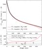 |
Fig. 1 Variation with height in the mean temperature ⟨ T ⟩ in several snapshots taken from the magneto-convection simulations with small-scale dynamo action by Rempel (2014). The ⟨ T ⟩ values correspond to the horizontal averages at each height in these snapshots. Top panel: temporal evolution of the mean temperature in time series snapshots with unsigned vertical mean field strength ⟨ | Bz | ⟩ = 80 G (thin gray curves). The curves are separated by a 120-solar-second time interval, and they cover 40 min of the stationary regime. Open red circles and red crosses indicate the snapshot models with ⟨ | Bz | ⟩ = 80 G and ⟨ | Bz | ⟩ = 0.5 G used in this study. Bottom panel: temperature differences Δ ⟨ T ⟩ between the two snapshot models with ⟨ | Bz | ⟩ = 80 G and ⟨ | Bz | ⟩ = 0.5 G (solid red curve). The dashed curve indicates the height variation of the standard deviation σ in the temperature, calculated from the spatially and temporally averaged value in the time series snapshots with ⟨ | Bz | ⟩ = 80. The second horizontal axis gives the mean optical depths log10 ⟨ τ5 ⟩ in the ⟨ | Bz | ⟩ = 80 G model of Rempel (2014), corresponding to the atmospheric heights given in the bottom horizontal axis. |
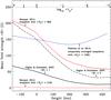 |
Fig. 2 Variation with height of the mean field strength ⟨ B ⟩ in several MHD models of the quiet solar photosphere. The black curves (solid and dashed-dotted) show the height variation of ⟨ B ⟩ that results from scaling factors F = 1 and F = 3 (see details in Shchukina & Trujillo Bueno 2011) of the magnetic strength in a MHD snapshot model resulting from the small-scale dynamo simulations by Vögler & Schüssler (2007). Red circles and crosses show the ⟨ B ⟩ values in the two snapshots we took from the small-scale dynamo simulations by Rempel (2014), with ⟨ | Bz | ⟩ = 80 G and ⟨ | Bz | ⟩ = 0.5 G. In both small-scale dynamo models, the net magnetic flux is zero. The thin blue solid curve corresponds to the time average of the ⟨ | Bz | ⟩ = 100 G model of Fabbian et al. (2012), which has a non-zero net flux and resulted from magneto-convection simulations without small-scale dynamo action. The top horizontal axis gives the mean optical depths log10 ⟨ τ5 ⟩ in the ⟨ | Bz | ⟩ = 80 G model of Rempel (2014), corresponding to the atmospheric heights given in the bottom horizontal axis. |
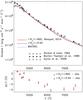 |
Fig. 3 Top panel: wavelength variation of calculated and observed absolute continuum intensities at the solar disk center. The solid red and black dashed curves correspond, respectively, to the ⟨ | Bz | ⟩ = 80 G and ⟨ | Bz | ⟩ = 0.5 G 3D snapshot models of Rempel (2014). The dotted blue line refers to the 1D MACKKL quiet-Sun model (Maltby et al. 1986). The symbols indicate the observational data from Neckel & Labs (1984; squares), Burlov-Vasiljev et al. (1998; black circles), and Ayres et al. (2006; stars). Bottom panel: relative differences between continuum intensities calculated using the 3D snapshot model of Rempel (2014) and observational data taken from Neckel & Labs (1984). Red circles with crosses and black crosses represent, respectively, the results obtained with the ⟨ | Bz | ⟩ = 80 G and ⟨ | Bz | ⟩ = 0.5 G snapshots. |
Figure 2 shows the height variation of the mean field strengths ⟨ B ⟩ in both 3D snapshots, which we obtained by averaging the magnetic strength at each height in the models. The mean field strength ⟨ B ⟩ is very close to zero in the snapshot with 0.5 G. Therefore, as mentioned above, we can consider this 3D model as unmagnetized. We provide two indications that the 3D model of Rempel (2014) with ⟨ | Bz | ⟩ = 80 G provides a reasonable representation of the magnetic properties in the quiet regions of the solar photosphere. Figure 2 shows that the mean magnetic field strength of the snapshot with ⟨ | Bz | ⟩ = 80 G is fairly close to the strength obtained from the model of Vögler & Schüssler (2007) if the magnetic strength of this model is scaled by a factor 3. Such scaling in the model of Vögler & Schüssler (2007) is needed to explain the Zeeman circular polarization signals of the Fe i lines at 6301.5 and 6302.5 Å observed with the Hinode space telescope (see Danilovic et al. 2010). It is also of interest that one of the models used by Fabbian et al. (2012) (i.e., the one with a vertical unsigned flux density of 100 G) gives a similar mean field strength in the low photospheric layers where the above-mentioned Zeeman signals originate (i.e., around 60 km according to Shchukina & Trujillo Bueno 2011).
Another indication that supports the reliability of the snapshot models of Rempel (2014) with ⟨ | Bz | ⟩ = 80 G and ⟨ | Bz | ⟩ = 0.5 G in the continuum-forming layers is the wavelength variation of the absolute continuum intensity at the solar disk center (see Fig. 3). The absolute continuum intensities computed in these snapshots are in good agreement and are also consistent with those calculated in the semi-empirical model MACKKL, which is based on observations of the continuum radiation. Therefore, the effective temperatures of the 3D snapshots we used in this investigation are virtually the same and in agreement with that of the above-mentioned solar semi-empirical model. The bottom panel of Fig. 3 shows that the relative differences between the absolute continuum intensity values calculated using the 3D snapshot model of Rempel (2014) and the observed intensities are in the range between +3% and −4%. These differences are smaller than the differences obtained by Fabbian et al. (2012) using their magneto-convection models without small-scale dynamo action (see their Fig. 2).
Finally, it should be noted that in Rempel’s (2014) model the mean field strength around 300 km above the visible “surface” is about a factor 2 smaller than the 130 G inferred by modeling the scattering polarization in the Sr i 4607 Å line using other 3D models of the quiet solar photosphere (see Trujillo Bueno et al. 2004; Shchukina & Trujillo Bueno 2011). Curiously, one of the magneto-convection models of Fabbian et al. (2012; i.e., their snapshot model characterized by a vertical unsigned flux density of 100 G) has a mean field strength ⟨ B ⟩ ≈ 130 G around a height of 300 km (Fig. 2).
2.2. Line parameters
Our Fe i line list is given in Table 1. For most of the lines we adopted the “solar” oscillator strengths and observed equivalent widths given by Gurtovenko & Kostik (1989). The only exception are four lines (5324.18, 5434.52, 5525.55, 6400.00 Å) selected from the “Kiel-Oxford line list” (Kostik et al. 1996) and two near-infrared lines 15 648.51 Å and 15 652.87 Å, whose “solar” oscillator strengths and equivalent widths were taken from Borrero et al. (2003). The 66 lines of Table 1 comprise a wide range of equivalent widths W (1.7−305 mÅ), wavelengths (4088.56−15 652.8 Å), excitation potentials of the lower level EPL (0.09−6.25 eV), and the Landé factor gL (0−3). Having so many clean, carefully chosen Fe i lines allows us to obtain statistically meaningful conclusions about possible differential abundance corrections due to the presence of a magnetic field. Fabbian et al. (2012) used 28 Fe i lines, 20% of which are strongly blended.
We used Voigt profiles for the absorption line shapes and define the damping constant γ as the sum of Van der Waals broadening γ6 and radiative broadening γrad. Our line list contains 26 lines, for which the Van der Waals broadening was evaluated using the semi-classical theory of Anstee, Barklem, and O’Mara, known as the ABO theory (see Anstee & O’Mara 1995; Barklem & O’Mara 1997; Barklem et al. 1998, and references therein). For the rest of the Fe i lines, we applied the classical Eq. (82,48) of Unsöld (1955) with the enhancement factor E = 1.5 recommended by Gurtovenko & Kostik (1989).
Our code for computing the background continuum opacity includes the equations of state for neutral hydrogen atoms, H− ions, protons, molecules  , H2 and for He, C, N, O, Ne, Na, Mg, Al, Si, P, S, Ar, Ca, Cr, Mn, Fe, Co, Ni atoms. We assumed the standard solar chemical composition given in Grevesse & Sauval (1998), which is in good agreement with the helioseismological data. For calculating the continuum absorption coefficient, we considerbound-free and free-free transitions in the H− ion and bound-free and free-free transitions in hydrogen. We have included also the contributions due to bound-free transitions in carbon, silicon, iron, magnesium, aluminum, Thomson scattering at free electrons, Rayleigh scattering from the ground level of neutral hydrogen. Likewise, we accounted for the UV haze opacity, which we calculated as explained in Bruls et al. (1992). More detailed information can be found in Kostik et al. (1996) and Trujillo Bueno & Shchukina (2009).
Since our goal here is to estimate differential abundance corrections, details, such as the enhancement factor choice and possible differences in the evaluation of the continuous opacity caused by employing our own opacity package instead of the one used in the 3D simulations, do not significantly affect the conclusions (see also Fabbian et al. 2012).
2.3. Method of analysis
To determine the abundance corrections due to the impact of the model’s magnetic field we have developed a radiative transfer code based on the DELOPAR method proposed by Trujillo Bueno (2003), which allows us to compute the emergent Stokes profiles by taking the Zeeman effect into account. We focus only on the emergent Stokes I(λ) profiles because this is the observable we use for determining the abundance corrections. The intensity profiles were calculated at the solar disk center assuming LTE for all the Fe i lines of Table 1 and at each point on the surface of the two 3D models used. The lines were synthesized with a spectral resolution depending on the line strength, varying between 2 mÅ for the weak lines and 15 mÅ for the strongest ones.
The resulting emergent intensity profiles of each Fe i line were spatially averaged over all surface points of the 3D atmospheric model under consideration, and for each Fe i line we computed the ensuing equivalent width W. Any difference between the observed equivalent width and the calculated one was ascribed to an incorrect iron abundance. We performed spectral synthesis of the Fe i lines and calculated their equivalent widths for several values of the iron abundance AFe, in the range between −0.1 and +0.1 dex relative to AFe = 7.50. For each Fe i line under consideration, the final value of the abundance corresponding to the observed equivalent width was determined by interpolating the intermediate equivalent widths obtained using varying abundances.
We also estimated the formation heights of the Fe i lines. We calculated them using the concept of “Eddington-Barbier height of line formation”; i.e., we calculated the continuum optical depth (τ5, at 5000 Å) where the line optical depth at a given line wavelength point Δλ is equal to unity. We repeated the calculations of τ5 values for all grid points of each 3D snapshot and then computed an average value ⟨ τ5 ⟩. We are fully aware of the practical limitations of this concept (e.g., Sánchez Almeida et al. 1996). However, from a statistical point of view, the concept of “the Eddington-Barbier height formation” is very appropriate.
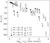 |
Fig. 4 Observed equivalent widths of the Fe i lines of Table 1 versus their mean line-center optical depths of formation, log10 ⟨ τ5(line center) ⟩, calculated using the ⟨ | Bz | ⟩ = 0.5 G snapshot. |
Figure 4 shows that the “heights of formation” of the Fe i lines of Table 1 cover a large region of the solar photosphere. This indicates that with the lines of Table 1, we can aim at finding some statistically significant height-dependent regularities, which are useful for a suitable quantification of the impact of the model’s magnetic field on the iron abundance determination.
We use abundance corrections (ΔA) for determining the direct and the indirect impact of photospheric magnetic fields on the solar iron abundance determination. We define ΔA = A(Bz = 80 G) − A(Bz = 0.5 G) as the difference between the abundances fitted using the 3D model snapshots with ⟨ | Bz | ⟩ = 80 G and ⟨ | Bz | ⟩ = 0.5 G. The indirect effect induced by changes in the thermodynamical structure of the atmosphere was found using the same 3D snapshots, but with zero magnetic field at each spatial grid point. To derive the direct impact caused by the Zeeman broadening produced by the model’s magnetic field, we calculated the differences between the abundances obtained from the ⟨ | Bz | ⟩ = 80 G snapshot and those obtained from the same snapshot but imposing B = 0 G.
We also estimated the effects of decreasing the horizontal resolution of the 3D snapshot models by comparing the abundance corrections obtained from several Fe i lines and considering the original horizontal resolution of 8 km and a coarser resolution of 80 km. We found that the ensuing changes in the abundance correction values are negligible and never exceed 10-4 dex.
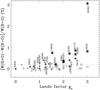 |
Fig. 5 Relative equivalent width changes of the Fe i lines, [W(B ≠ 0) − W(B = 0)] /W(B = 0), caused by the direct Zeeman broadening effect versus the line’s effective Lande factor gL. The equivalent widths W(B ≠ 0) and W(B = 0) were calculated using, respectively, the ⟨ | Bz | ⟩ = 80 G snapshot model and the same model assuming B = 0 G at each grid point. See Fig. 4 for further information. |
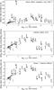 |
Fig. 6 Relative changes, in percentage, of the Fe i equivalent widths ΔW/W caused by the impact of the model’s magnetic field versus the mean line-center optical depths. The ⟨ τ5(line center) ⟩ values have been calculated at the line center of the lines using the snapshot with ⟨ | Bz | ⟩ = 0.5 G. Top panel: direct effect due to the ensuing Zeeman broadening of the Fe i lines. The equivalent width changes [W(B ≠ 0) − W(B = 0)] /W(B = 0) are the same as in Fig. 5. Middle panel: indirect effect caused by the magnetically induced changes of the thermodynamical properties in the formation region of the Fe i lines. Bottom panel: joint action of the direct and indirect effects. |
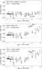 |
Fig. 7 Impact of the small-scale magnetic fields of Rempel’s (2014) model on the determination of the solar iron abundance. Top panel: corrections of the Fe i abundances due to the direct Zeeman broadening effect on the Fe i lines. Middle panel: corrections of the Fe i abundances caused by the magnetically induced changes of thermodynamical properties of the solar photosphere in the line formation regions. Bottom panel: combined effect representing the sum of the ΔA values shown in the top and middle panels. The abundance corrections are given against the mean line-center optical depths of the Fe i lines calculated in the 3D model snapshot with ⟨ | Bz | ⟩ = 0.5 G. The mean of the abundance corrections, ⟨ ΔA ⟩, and their corresponding rms values are shown in the upper left corner of each panel. |
3. Results
3.1. The impact of the direct effect
Figure 5 shows the influence of the direct effect (magnetic Zeeman broadening) on the equivalent widths W of the Fe i lines of Table 1 as a function of their effective Landé factor gL. We estimated the impact of this effect by calculating the relative changes ΔW/W = [W(B ≠ 0) − W(B = 0)] /W(B = 0) of the W-values, using the 3D snapshot model with ⟨ | Bz | ⟩ = 80 G and the same one with B = 0 G at each grid point. Considering that the magnetic sensitivity of the Fe i lines increases not only with gL but also with wavelength and the magnetic field strength in the line formation region (Landi Degl’Innocenti & Landolfi 2004), the dependence between ΔW/W and the line’s Landé factor is not as straightforward as might be expected. In fact, all Fe i lines used in our study can be subdivided into four sets depending on their W and gL values.
The lines of the first two sets shown in Figs. 4 and 5 by circles and squares are relatively weak (W< 40 mÅ). Moreover, the first set of lines is characterized by relatively low values of the effective Landé factor (gL ≤ 1.5). The second set of lines has gL> 1.5. In general, for both sets the changes of the equivalent widths due to the direct Zeeman broadening effect are very modest. They never exceed 0.2% for the Fe i lines with gL ≤ 1.5, while the ΔW/W-values for the lines of the second set slightly increase with equivalent width and effective Landé factor (e.g., the Fe i lines at 5784.66 Å and 6733.16 Å).
The third and fourth sets contain moderate and strong Fe i lines (with W> 40 mÅ). The third set contains lines with gL ≤ 1.5 (see crosses in Figs. 4 and 5). The fourth set comprises lines with effective Landé factors larger than 1.5 (see filled circles surrounded by open circles). Interestingly, the lines of the third set exceed the threshold ΔW/W = 0.2% only if their wavelengths are longer than 5705 Å, and their equivalent widths lie between 40 mÅ and 130 mÅ (e.g., the Fe i lines at 5705.46, 6240.65, 6297.80, 6430.85, 6593.87 Å). Nevertheless, the ΔW/W-values of these lines remain below 0.5%. The fourth set of Fe i lines demonstrates a clear trend of enhanced magnetic sensitivity with increasing Landé factor. For the optical lines of this set, the equivalent width changes can reach 0.9%. The infrared lines at 15 648.5 Å and 15 652.9 Å do not behave in the same way because of their extra sensitivity resulting from their longer wavelengths. The first of these lines has Landé factor gL = 3 and, as a result, the highest magnetic sensitivity (ΔW/W ≈ 3%).
The top panel of Fig. 6 shows that equivalent width changes ΔW/W caused by the Zeeman broadening effect depend on the mean optical depth of the above-mentioned line-center formation height, ⟨ τ5(line center) ⟩. There is a clear indication of the impact of the magnetic field on the equivalent widths of the Fe i lines in the range 0 < log10 ⟨ τ5(line center) ⟩ ≤ − 3. The infrared 15 648.5 Å line shows a rather large change in the equivalent width, which lies well outside the general behavior observed in the other Fe i lines. The Fe i lines originating in the higher photospheric layers, where the model’s magnetic field is weaker, are rather insensitive to the ensuing magnetic broadening.
The abundance corrections ΔA determined from such equivalent width changes are shown in the top panel of Fig. 7. As seen in this figure, ΔA ≤ 0 for all Fe i lines from Table 1. Therefore, abundance determinations carried out ignoring the Zeeman broadening of the photospheric Fe i lines tend to overestimate the AFe value. The most magnetically sensitive line (i.e., the 15 648.5 Å line) gives the largest abundance error, namely −0.02 dex. The errors for other magnetically sensitive lines in Fig. 7 with filled circles are even smaller. On average, the direct impact of the small-scale magnetic fields of Rempel’s (2014) model on the determination of the solar iron abundance is negligibly small. For the lines used in our study, the mean value of the abundance corrections is only ⟨ ΔA ⟩ = − 0.002 ± 0.004 dex.
3.2. The impact of the indirect effect
Indirect magnetic effects on the spectral lines of different chemical elements occur because of changes in the thermodynamical structure caused by the presence of the magnetic field. In the Fe i lines used for the abundance determinations, changes in their equivalent widths are mainly produced by the temperature changes (Holweger & Testerman 1975; Rutten 1988; Gray 1992; Shchukina & Trujillo Bueno 2001).
The solid curve of Fig. 8 shows the magnetically-induced changes of the temperature variations Δ ⟨ T ⟩ = ⟨ T( | Bz | = 80G) ⟩ − ⟨ T( | Bz | = 0.5G) ⟩ between the ⟨ | Bz | ⟩ = 80 G and ⟨ | Bz | ⟩ = 0.5 G snapshot models versus the optical depth τ5. We obtained these changes after averaging the temperature of each of the snapshot models over surfaces of equal τ5-values. This curve corresponds to the solid curve shown in the bottom panel of Fig. 1, but now it is plotted against the optical depth τ5.
For each Fe i line of Table 1, we also calculated the mean temperatures ⟨ Tline( | Bz | = 80G) ⟩ and ⟨ Tline( | Bz | = 0.5G) ⟩ and the mean optical depths ⟨ τ5(line center) ⟩, which allowed us to estimate where the line-center intensity of the Fe i lines is formed. We derived these values using the concept of “Eddington-Barbier heights of line formation”; i.e. we calculated the temperature Tline and the continuum optical depth τ5(line center) where the optical depth τΔλ at the line center Δλ = 0 is equal to unity. We repeated the calculations of Tline and τ5(line center) for all grid points of each 3D snapshot and then computed an average value ⟨ Tline ⟩ and ⟨ τ5(line center) ⟩. The differences Δ ⟨ Tline ⟩ = ⟨ Tline( | Bz | = 80 G) ⟩ − ⟨ Tline( | Bz | = 0.5 G) ⟩ for the four sets of the Fe i lines discussed in Sect. 3.1 are shown in Fig. 8 against the mean line-center optical depths ⟨ τ5(line center) ⟩ , which we calculated using the ⟨ | Bz | ⟩ = 0.5 G snapshot model.
As seen in Fig. 8, the temperature changes Δ ⟨ T ⟩ are the largest in the higher photospheric layers of Rempel’s (2014) model, with values exceeding 100 K. For those Fe i lines whose line center radiation comes from atmospheric layers with log10τ5 = 0 and −3, the temperature changes between the snapshot models with ⟨ | Bz | ⟩ = 80 G and ⟨ | Bz | ⟩ = 0.5 G are rather modest. We point out that these deviations are smaller than those of the 3D magneto-convection models used by Fabbian et al. (2010, 2012). At atmospheric layers with log10τ5< − 3, however, the temperature changes between the magnetized and unmagnetized models of Rempel (2014) are larger.
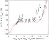 |
Fig. 8 Δ ⟨ T ⟩ changes of the temperature stratifications of the ⟨ | Bz | ⟩ = 80 G and ⟨ | Bz | ⟩ = 0.5 G snapshots versus the optical depth τ5 (solid red line). The Δ ⟨ T ⟩ values have been obtained after averaging the temperature over surfaces of equal optical depth τ5. The symbols indicate the differences between the mean temperatures Δ ⟨ Tline ⟩ in the formation layers of the Fe i line centers derived for the same snapshots; they are given against the mean line center optical depths ⟨ τ5(line center) ⟩ calculated in the ⟨ | Bz | ⟩ = 0.5 G snapshot. Circles, squares, crosses, and filled circles denote the same sets of lines as in Fig. 4. The symbols with triangles indicate the mean optical depths where the Fe i line wings originate. |
The variation with optical depth of the mean temperature differences Δ ⟨ Tline ⟩ in the line cores of the Fe i lines follows the temperature differences Δ ⟨ T ⟩ quite well between the two snapshots. The only exception is for the 5247.05, 5225.53, and 5250.21 Å lines with a low value of the excitation potential (0.09 ≤ EPL ≤ 0.12 eV), which deviate significantly from the solid curve. Figures 9 and 10 help to explain the anomalies of such behavior. The top and bottom panels of these figures show the histograms, respectively, of the optical depths τ5(line center) and the temperatures in the core formation layers of the Fe i 6302.50 Å and 5250.21 Å lines. As a typical representative of the lines shown in Fig. 8, the Fe i 6302.50 line is formed in a rather thin layer compared with the “abnormal” 5250.21 Å line. In addition, the distribution of the line-center optical depths τ5(line center) for the 6302.50 Å line in both snapshots is similar, resulting in almost the same mean optical depths of the line core (see top panel of Fig. 9). The bottom panel of this figure demonstrates that the temperature structure in the line-center formation regions of these models is also quite similar. As a consequence, the mean difference Δ ⟨ Tline ⟩ is fairly close to the temperature difference Δ ⟨ T ⟩ between the two snapshots at the mean optical depth ⟨ τ5(line center) ⟩.
The top panel of Fig. 10 shows that, in contrast to the 6302.50 Å line, the 5250.21 Å line originates in a more extended region. (The same happens with other lines with a low value of the EPL, like the 5225.53 Å and 5247.05 Å lines.) In the ⟨ | Bz | ⟩ = 80 G 3D snapshot model, its radiation comes on average from deeper layers than in the unmagnetized model. For this reason, the mean temperature in the formation region of the Fe i 5250.21 Å line in the ⟨ | Bz | ⟩ = 80 G snapshot model turns out to be appreciably larger (see bottom panel of Fig. 10).
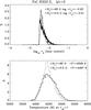 |
Fig. 9 Histograms of the logarithmic optical depths log10τ5(line center) (top panel) and of the temperatures (bottom panel) at the photospheric layers where the line center of the Fe i 6302.50 Å is formed. Solid and dotted curves show results, respectively, for the 3D model snapshots with ⟨ | Bz | ⟩ = 80 G and ⟨ | Bz | ⟩ = 0.5 G. The mean values of the temperature and optical depth are shown, respectively, in the upper right and upper left corners of the corresponding panels. |
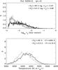 |
Fig. 10 Histograms of the logarithmic optical depths log10τ5(line center) (top panel) and the temperatures (bottom panel) at the photospheric layers where the line center of the Fe i 5250.21 Å is formed. See the legend of Fig. 9 for further information. |
Interestingly, the Fe i lines forming in deep photospheric layers, such as the infrared 15 648.5 Å, 15 652.9 Å lines and the optical 5784.66 Å, 5827.87 Å, 6733.16 Å lines, also display rather noticeable deviations from the solid curve in Fig. 8. In these layers the temperature increases rapidly with depth, so even relatively small shifts in the line formation layer cause appreciably larger deviations of the Δ ⟨ Tline( | Bz | = 80G) ⟩ values from the Δ ⟨ T ⟩ curve.
The temperature differences shown in Fig. 8 imply equivalent width changes and corresponding abundance corrections. We show them in the middle panels of Figs. 6 and 7. As can be seen in these figures, the indirect impact of the surface dynamo magnetic fields on the determination of the solar iron abundance is much more pronounced than the direct one. In the ⟨ | Bz | ⟩ = 80 G snapshot, the Fe i lines from Table 1 become weaker (see the middle panel of Fig. 6). The only exception is the 4091.56 Å line that shows a slight increase in its equivalent width. This sort of weakening depends strongly on the mean optical depths ⟨ τ5(line center) ⟩. The sensitivity of the equivalent widths of weaker Fe i lines (W< 40 mÅ) emerging from the deeper layers below ⟨ τ5(line center) ⟩ = − 1.1 decreases with decreasing the mean line optical depth, while for the lines with W> 40 mÅ and ⟨ τ5(line center) ⟩ < − 1.3, the opposite effect takes place. The maximum changes in the equivalent widths for the weakest and strongest Fe i lines used in our study reach 4%. The lines with W> 40 mÅ, whose line cores originate in the intermediate layers (−1.3 < ⟨ τ5(line center) ⟩ < − 2.6), are less affected by the temperature effects. As we can see, their equivalent widths are reduced by less than 1%.
The line weakenings shown in the middle panel of Fig. 6 indicate that abundance determinations that ignore the magnetically induced changes in the solar atmospheric structure underestimate the AFe-value. The middle panel of Fig. 7 shows that the abundance corrections ΔA related to the equivalent width changes displayed in the middle panel of Fig. 6 are positive for all Fe i lines of Table 1, except for the 4091.56 Å line, which has a small negative abundance correction (ΔA< − 0.005 dex). There is no clear dependence of the abundance corrections ΔA on the mean line optical depth for the lines forming below ⟨ τ5(line center) ⟩ = − 2. Their ΔA values, as well as those of the infrared 15 648.5 Å, 15 652.9 Å lines, never exceed 0.02 dex. Unlike these lines the abundance corrections for the lines emerging from higher layers gradually increase with decreasing mean line optical depth, starting with ~0.01 dex for the 6173.34 Å line and ending with ~0.045 dex for the strong 5434.52 Å line. The lines with a low value of the EPL (5247.05 Å, 5250.21 Å, 5225.53 Å) fall outside this dependence. Their ΔA values are the highest (0.05 − 0.07 dex). A careful comparison of the middle and top panels of Fig. 7 shows that the mean of the abundance corrections needed to take the indirect effects into account is almost an order of magnitude greater than the abundance corrections coming from the direct effect. Nevertheless, the mean error of the iron abundance determinations that ignore the magnetically induced changes in the temperature structure of the solar atmosphere remains very small: ⟨ ΔA ⟩ = + 0.016 ± 0.012 dex.
3.3. The joint impact of the direct and indirect effects
The bottom panel of Fig. 6 shows the joint action of the direct and indirect effects on the Fe i line equivalent widths. The ensuing abundance corrections are given in Table 1 and are shown in the bottom panel of Fig. 7. Since the direct and indirect effects act in opposite ways, their joint influence reduces the impact of the local dynamo magnetic fields on the Fe i line equivalent widths and, therefore, on the determination of the iron abundance. As we have seen, the Zeeman broadening effect remains weak for most of the Fe i lines of Table 1. Therefore, the direct effect is unable to compensate for the indirect temperature effect. Nevertheless, there are three lines with large Landé factor for which both effects are comparable. They are the 15 648.5 Å, 6173.34 Å, and 6302.50 Å lines, for which the abundance corrections vary only from −0.008 dex to +0.006 dex. Summarizing, we conclude that in Rempel’s (2014) model, the impact on the iron abundance caused by the joint action of the direct and indirect effects is negligible, namely ⟨ ΔA ⟩ = + 0.014 ± 0.011 dex.
4. Conclusions
The aim of this paper has been to quantify the possible impact of the small-scale magnetic fields of the quiet solar photosphere on the determination of the iron abundance, considering the direct effect due to the Zeeman broadening of the intensity profiles and the indirect effect caused by magnetic field induced changes in the thermodynamical structure of the photospheric plasma. To this end, we have carried out LTE spectral synthesis in unmagnetized and magnetized 3D models of the solar photosphere, in order to compare the calculated and observed equivalent widths in the 66 Fe i lines given in Table 1. However, instead of adopting magneto-convection models without small-scale dynamo action and non-zero values of the net magnetic flux, such as those used by Fabbian et al. (2012), we used two 3D snapshot models resulting from the magneto-convection simulations with small-scale dynamo action carried out by Rempel (2014). One of the snapshot models we used is virtually unmagnetized, while the other (corresponding to the stationary stage of the simulation) has ⟨ | Bz | ⟩ = 80 G and ⟨ B ⟩ = 160 G in the visible surface layers (see Fig. 2). In this significantly magnetized model of the quiet solar photosphere the net magnetic flux is zero.
The 66 Fe i lines of Table 1 span a wide range in wavelength, oscillator strength, and effective Landé factor. These spectral lines originate in a large domain of the solar photosphere. For each Fe i line we determined differential abundance corrections by comparing with observations the equivalent widths of the emergent intensity profiles calculated in the two 3D snapshot models. Given the statistical significance of our line list, we could obtain optical-depth dependent regularities in our quantification of the impact of the model’s small-scale dynamo magnetic fields on the solar Fe i abundance determination. Our conclusion is that if the magnetism of the quiet solar photosphere is mainly produced by a small-scale dynamo, then its impact on the determination of the solar iron abundance is negligible.
We support the conclusion of Fabbian et al. (2010, 2012) that the indirect effect of magnetic fields on the iron abundance determination is on average significantly larger than the direct effect caused by the line Zeeman broadening. However, in Rempel’s (2014) small-scale dynamo model (whose ⟨ B ⟩ = 160 G), these effects are rather negligible. In Table 1 there are 11 Fe i lines that are also present in the list of 28 lines chosen by Fabbian et al. (2012; see the lines labeled by the letter “F”). The average abundance corrections due to the joint action of the direct and indirect effects is 0.018 dex (when using Rempel’s 2014 model) and 0.036 dex (when using the 100 G model of Fabian et al.). We point out that there are three lines with a low value of the EPL (5225.53, 5247.05, 5250.21 Å), which have an appreciably higher sensitivity to the presence of small-scale photospheric magnetic fields. In Rempel’s (2014) model, the average effect for these spectral lines reaches ~0.05 dex, while it is ~0.08 dex and ~0.11 dex in the 100 G and 200 G models of Fabbian et al. (2012), respectively. Therefore, we recommend avoiding using such lines when determining the solar iron abundance.
When the complete set of lines of Table 1 is used, we find that the influence of the small-scale magnetic fields of Rempel’s (2014) model on the iron abundance determination is smaller than +0.014 dex. This value is approximately three times smaller than the one obtained by Fabbian et al. (2012) from 28 Fe i lines on the basis of their 3D magneto-convection model with ⟨ | Bz | ⟩ = 100 G.
Online material
Fe i line list.
Acknowledgments
We are very grateful to M. Rempel (HAO) for kindly providing the 3D model atmospheres weused in this investigation and for helpful scientific discussions. Thanks are also due to D. Fabbian, E. Khomenko and F. Moreno-Insertis for scientificconversations. Financial support by the Spanish Ministry of Economy and Competitiveness (MINECO) through projects AYA2010–18029 (Solar Magnetism and Astrophysical Spectropolarimetry) and AYA2014-55078-P (The Solar Atmosphere: theory, computing tools and support to observations) are gratefully acknowledged. N. Shchukina is also grateful to the MINECO, through the 2011 Severo Ochoa Program SEV-2011-0187, which granted her a sabbatical stay at the IAC.
References
- Anstee, S. D., & O’Mara, B. J. 1995, MNRAS, 276, 859 [NASA ADS] [CrossRef] [Google Scholar]
- Asplund, M. 2000, A&A, 359, 755 [NASA ADS] [Google Scholar]
- Asplund, M., Nordlund, Å., Trampedach, R., Allen de Prieto, C., & Stein, R. F. 2000a, A&A, 359, 729 [NASA ADS] [Google Scholar]
- Asplund, M., Nordlund, Å., Trampedach, R., & Stein, R. F. 2000b, A&A, 359, 743 [NASA ADS] [Google Scholar]
- Asplund, M., Grevesse, N., & Sauval, A. J. 2005a, in Cosmic Abundances as Records of Stellar Evolution and Nucleosynthesis, eds. F. N. Bash, & T. G. Barnes (San Francisco: ASP), ASP Conf. Ser., 336, 25 [Google Scholar]
- Asplund, M., Grevesse, N., Sauval, A. J., Allen de Prieto, C., & Blomme, R. 2005b, A&A, 431, 693 [NASA ADS] [CrossRef] [EDP Sciences] [Google Scholar]
- Asplund, M., Grevesse, N., Sauval, A. J., & Scott, P. 2009, ARA&A., 47, 481 [NASA ADS] [CrossRef] [Google Scholar]
- Athay, R. G., & Lites, B. W. 1972, ApJ, 176, 809 [NASA ADS] [CrossRef] [Google Scholar]
- Atroshchenko, I. N., & Gadun, A. S. 1994, A&A, 291, 635 [NASA ADS] [Google Scholar]
- Ayres, T. R., Plymate, C., & Keller, C. U. 2006, ApJ, 165, 618 [Google Scholar]
- Bahcall, J. N., Basu, S., Pinsonneault, M., & Serenelli, A. M. 2005, ApJ, 618, 1049 [NASA ADS] [CrossRef] [Google Scholar]
- Barklem, P. S., & O’Mara, B. J. 1997, MNRAS, 290, 102 [Google Scholar]
- Barklem, P. S., O’Mara, B. J., & Ross, J. E. 1998, MNRAS, 296, 1057 [Google Scholar]
- Basu, S., & Antia, H. M. 2008, Phys. Rep., 457, 217 [NASA ADS] [CrossRef] [Google Scholar]
- Blackwell, D. E., Booth, A., & Petford, A. 1984, A&A, 236, 239 [Google Scholar]
- Borrero, J. M. 2008, ApJ, 673, 470 [NASA ADS] [CrossRef] [Google Scholar]
- Borrero, J. M., Bellot Rubio, L. R., Barklem, P. S., & del Toro Iniesta, J. C. 2003, A&A, 404, 749 [NASA ADS] [CrossRef] [EDP Sciences] [Google Scholar]
- Brandenburg, A. 2011, ApJ, 741, 92 [NASA ADS] [CrossRef] [Google Scholar]
- Bruls, J. H. M. J., Rutten, R. J., & Shchukina, N. 1992, A&A, 265, 237 [NASA ADS] [Google Scholar]
- Buehler, D., Lagg, A., & Solanki, S. K. 2013, A&A, 555, A33 [NASA ADS] [CrossRef] [EDP Sciences] [Google Scholar]
- Burlov-Vasiljev, K. A., Matveev, Ya. B., & Vasiljeva, I. E. 1998, Sol. Phys., 177, 25 [NASA ADS] [CrossRef] [Google Scholar]
- Caffau, E., Ludwig, H.-G., Steffen, M., et al. 2008, A&A, 488, 1031 [CrossRef] [EDP Sciences] [Google Scholar]
- Caffau, E., Ludwig, H.-G., Steffen, M., Freytag, B., & Bonifacio, P. 2011, Sol. Phys., 268, 255 [NASA ADS] [CrossRef] [Google Scholar]
- Cattaneo, F. 1999, ApJ, 515, L39 [NASA ADS] [CrossRef] [Google Scholar]
- Danilovic, S., Schüssler, M., & Solanki, S. K. 2010, A&A, 513, A1 [NASA ADS] [CrossRef] [EDP Sciences] [Google Scholar]
- Deinzer, W., Hensler, G., Schüssler, M., & Weisshaar, E. 1984, A&A, 139, 435 [NASA ADS] [Google Scholar]
- Fabbian, D., Khomenko, E., Moreno-Insertis, F., & Nordlund, Å. 2010, ApJ, 724, 1536 [NASA ADS] [CrossRef] [Google Scholar]
- Fabbian, D., Moreno-Insertis, F., Khomenko, E., & Nordlund, Å. 2012, A&A, 548, A35 [NASA ADS] [CrossRef] [EDP Sciences] [Google Scholar]
- Fabiani Bendicho, P., Kneer, F., & Trujillo Bueno, J. 1992, A&A, 264, 229 [NASA ADS] [Google Scholar]
- Gray, D. F. 1992, The observation and analysis of stellar photospheres, Camb. Astrophys. Ser., 20 [Google Scholar]
- Grevesse, N., & Sauval, A. J. 1998, in Solar Composition and Its Evolution – from Core to Corona, eds. C. Frolich, M. Huber, S. K. Solanki, & R. von Steiger (Dordrecht: Kluwer), 161 [Google Scholar]
- Gurtovenko, E. A., & Kostik, R. I. 1989, Fraunhofer Spectrum and the System of Solar Oscillator Strengths (Kiev: Izdatel’otvo Naukova Dumka), Naukova Dumka [Google Scholar]
- Holweger, H., & Testerman, L. 1975, Sol. Phys., 43, 271 [NASA ADS] [CrossRef] [Google Scholar]
- Holweger, H., Heise, C., & Kock, M. 1990, A&A, 232, 510 [NASA ADS] [Google Scholar]
- Ishikawa, R., & Tsuneta, S., 2009, A&A, 495, 607 [NASA ADS] [CrossRef] [EDP Sciences] [Google Scholar]
- Kostik, R. I., Shchukina, N., & Rutten, R. J. 1996, A&A, 325, 342 [Google Scholar]
- Landi Degl’Innocenti, E., & Landolfi, M. 2004, Polarization in Spectral Lines (Kluwer Academic Publishers) [Google Scholar]
- Lites, B. W. 2011, ApJ, 737, 52 [NASA ADS] [CrossRef] [Google Scholar]
- Lodders, K. 2003, ApJ, 591, 1220 [NASA ADS] [CrossRef] [Google Scholar]
- Lodders, K., Palme, H., & Gail, H.-P. 2009, in Landolt-Börnstein, New Series, Vol. VI/4B, Chap. 4.4, Abundances of the Elements in the Solar System, ed. J. E. Trümper (Berlin, Springer-Verlag), 560 [Google Scholar]
- Maltby, P., Avrett, E. H., Carlsson, M., et al. 1986, ApJ, 306, 284 [Google Scholar]
- Martínez Pillet, V. 2013, Space Sci. Rev., 178, 141 [NASA ADS] [CrossRef] [Google Scholar]
- Neckel, H., & Labs, D. 1984, Sol. Phys., 90, 205 [NASA ADS] [CrossRef] [Google Scholar]
- Pereira, T. M. D., Asplund, M., Collet, R., et al. 2013, A&A, 554, A118 [NASA ADS] [CrossRef] [EDP Sciences] [Google Scholar]
- Petrovay, K., & Szakaly, G. 1993, A&A, 274, 543 [Google Scholar]
- Pietarila Graham, J., Cameron, R., & Schüsssler, M. 2010, ApJ, 714, 1606 [NASA ADS] [CrossRef] [Google Scholar]
- Rempel, M. 2014, ApJ, 789, 132 [NASA ADS] [CrossRef] [Google Scholar]
- Rutten, R. J. 1988, in IAU Colloq. 94, Physics of Formation of Fe ii Lines Outside LTE, eds. R. Viotti, A. Vittone, & M. Friedjung (Dordrecht: Reidel), 185 [Google Scholar]
- Rutten, R. J., & Kostik, R. I. 1982, A&A, 115, 104 [NASA ADS] [Google Scholar]
- Sánchez Almeida, J., Ruiz Cobo, B., & del Toro Iniesta, J. C. 1996, A&A, 314, 295 [NASA ADS] [Google Scholar]
- Sánchez Almeida, J., & Martínez González, M. 2011, in Solar Polarization 6, eds. J. R. Kuhn, D. M. Harrington, H. Lin, et al. (San Francisco: ASP), ASP Conf. Ser., 437, 451 [Google Scholar]
- Schekochihin, A. A., Iskakov, A. B., Cowley, S. C., et al. 2007, New J. Phys., 9, 300 [Google Scholar]
- Scott, P., Grevesse, N., Asplund, M., et al. 2015a, A&A, 573, A25 [NASA ADS] [CrossRef] [EDP Sciences] [Google Scholar]
- Scott, P., Asplund, M., Grevesse, N., Bergemann, M., & Sauval, A. J. 2015b, A&A, 573, A26 [NASA ADS] [CrossRef] [EDP Sciences] [Google Scholar]
- Serenelli, A. M., Basu, S., Ferguson, J. W., & Asplund, M. 2009, ApJ, 705, L123 [NASA ADS] [CrossRef] [Google Scholar]
- Shchukina, N., & Trujillo Bueno, J. 1998, Kinemat Phys. Celest. Bodies, 14, 242 [NASA ADS] [Google Scholar]
- Shchukina, N., & Trujillo Bueno, J. 2001, ApJ, 550, 970 [NASA ADS] [CrossRef] [Google Scholar]
- Shchukina, N., & Trujillo Bueno, J. 2009, in Solar Polarization 5, eds. S. Berdyugina, K. N. Nagendra, & R. Ramelli (San Francisco: ASP), ASP Conf. Ser., 405, 275 [Google Scholar]
- Shchukina, N., & Trujillo Bueno, J. 2011, ApJ, 731, L21 [NASA ADS] [CrossRef] [Google Scholar]
- Shchukina, N., Trujillo Bueno, J., & Asplund, M. 2005, ApJ, 618, 939 [NASA ADS] [CrossRef] [Google Scholar]
- Shchukina, N., Olshevsky, V. L., & Khomenko, E. V. 2009, A&A, 506, 1393 [NASA ADS] [CrossRef] [EDP Sciences] [Google Scholar]
- Shchukina, N., Sukhorukov, A., & Trujillo Bueno, J. 2012, ApJ, 755, 176 [NASA ADS] [CrossRef] [Google Scholar]
- Stein, R. F., & Nordlund, Å. 1998, ApJ, 499, 914 [Google Scholar]
- Stenflo, J. O. 2012, A&A, 547, A11 [Google Scholar]
- Stenflo, J. O. 2013, A&ARv, 21, 66 [NASA ADS] [CrossRef] [EDP Sciences] [Google Scholar]
- Sukhorukov, A. V. 2012, J. Phys. Studies, 6, 1903 [Google Scholar]
- Thévenin, F., & Idiart, T. 1999, ApJ, 521, 753 [NASA ADS] [CrossRef] [Google Scholar]
- Trampedach, R., Asplund, M., Collet, R., Nordlund, Å., & Stein, R. F. 2013, ApJ, 768, 18 [NASA ADS] [CrossRef] [Google Scholar]
- Trujillo Bueno, J. 2003, in Stellar Atmosphere Modeling, eds. I. Hubeny, D. Mihalas & K. Werner, ASP Conf. Ser., 288, 551 [Google Scholar]
- Trujillo Bueno, J., & Shchukina, N. 2007, ApJ, 664, L135 [NASA ADS] [CrossRef] [Google Scholar]
- Trujillo Bueno, J., & Shchukina, N. 2009, ApJ, 694, 1364 [NASA ADS] [CrossRef] [Google Scholar]
- Trujillo Bueno, J., Shchukina, N., & Asensio Ramos, A. 2004, Nature, 430, 326 [Google Scholar]
- Trujillo Bueno, J., Asensio Ramos, A., & Shchukina, N. 2006, in Solar Polarization 4, eds. R. Casini & B. W. Lites (San Francisco: ASP), ASP Conf. Ser., 358, 269 [Google Scholar]
- Unsöld, A. 1955, Physik der Sternatmosphären, 2nd edn. (Berlin: Springer Verlag [Google Scholar]
- Vögler, A., & Schüssler, M. 2007, A&A, 465, L43 [NASA ADS] [CrossRef] [EDP Sciences] [Google Scholar]
All Tables
All Figures
|
Fig. 1 Variation with height in the mean temperature ⟨ T ⟩ in several snapshots taken from the magneto-convection simulations with small-scale dynamo action by Rempel (2014). The ⟨ T ⟩ values correspond to the horizontal averages at each height in these snapshots. Top panel: temporal evolution of the mean temperature in time series snapshots with unsigned vertical mean field strength ⟨ | Bz | ⟩ = 80 G (thin gray curves). The curves are separated by a 120-solar-second time interval, and they cover 40 min of the stationary regime. Open red circles and red crosses indicate the snapshot models with ⟨ | Bz | ⟩ = 80 G and ⟨ | Bz | ⟩ = 0.5 G used in this study. Bottom panel: temperature differences Δ ⟨ T ⟩ between the two snapshot models with ⟨ | Bz | ⟩ = 80 G and ⟨ | Bz | ⟩ = 0.5 G (solid red curve). The dashed curve indicates the height variation of the standard deviation σ in the temperature, calculated from the spatially and temporally averaged value in the time series snapshots with ⟨ | Bz | ⟩ = 80. The second horizontal axis gives the mean optical depths log10 ⟨ τ5 ⟩ in the ⟨ | Bz | ⟩ = 80 G model of Rempel (2014), corresponding to the atmospheric heights given in the bottom horizontal axis. |
| In the text | |
|
Fig. 2 Variation with height of the mean field strength ⟨ B ⟩ in several MHD models of the quiet solar photosphere. The black curves (solid and dashed-dotted) show the height variation of ⟨ B ⟩ that results from scaling factors F = 1 and F = 3 (see details in Shchukina & Trujillo Bueno 2011) of the magnetic strength in a MHD snapshot model resulting from the small-scale dynamo simulations by Vögler & Schüssler (2007). Red circles and crosses show the ⟨ B ⟩ values in the two snapshots we took from the small-scale dynamo simulations by Rempel (2014), with ⟨ | Bz | ⟩ = 80 G and ⟨ | Bz | ⟩ = 0.5 G. In both small-scale dynamo models, the net magnetic flux is zero. The thin blue solid curve corresponds to the time average of the ⟨ | Bz | ⟩ = 100 G model of Fabbian et al. (2012), which has a non-zero net flux and resulted from magneto-convection simulations without small-scale dynamo action. The top horizontal axis gives the mean optical depths log10 ⟨ τ5 ⟩ in the ⟨ | Bz | ⟩ = 80 G model of Rempel (2014), corresponding to the atmospheric heights given in the bottom horizontal axis. |
| In the text | |
|
Fig. 3 Top panel: wavelength variation of calculated and observed absolute continuum intensities at the solar disk center. The solid red and black dashed curves correspond, respectively, to the ⟨ | Bz | ⟩ = 80 G and ⟨ | Bz | ⟩ = 0.5 G 3D snapshot models of Rempel (2014). The dotted blue line refers to the 1D MACKKL quiet-Sun model (Maltby et al. 1986). The symbols indicate the observational data from Neckel & Labs (1984; squares), Burlov-Vasiljev et al. (1998; black circles), and Ayres et al. (2006; stars). Bottom panel: relative differences between continuum intensities calculated using the 3D snapshot model of Rempel (2014) and observational data taken from Neckel & Labs (1984). Red circles with crosses and black crosses represent, respectively, the results obtained with the ⟨ | Bz | ⟩ = 80 G and ⟨ | Bz | ⟩ = 0.5 G snapshots. |
| In the text | |
|
Fig. 4 Observed equivalent widths of the Fe i lines of Table 1 versus their mean line-center optical depths of formation, log10 ⟨ τ5(line center) ⟩, calculated using the ⟨ | Bz | ⟩ = 0.5 G snapshot. |
| In the text | |
|
Fig. 5 Relative equivalent width changes of the Fe i lines, [W(B ≠ 0) − W(B = 0)] /W(B = 0), caused by the direct Zeeman broadening effect versus the line’s effective Lande factor gL. The equivalent widths W(B ≠ 0) and W(B = 0) were calculated using, respectively, the ⟨ | Bz | ⟩ = 80 G snapshot model and the same model assuming B = 0 G at each grid point. See Fig. 4 for further information. |
| In the text | |
|
Fig. 6 Relative changes, in percentage, of the Fe i equivalent widths ΔW/W caused by the impact of the model’s magnetic field versus the mean line-center optical depths. The ⟨ τ5(line center) ⟩ values have been calculated at the line center of the lines using the snapshot with ⟨ | Bz | ⟩ = 0.5 G. Top panel: direct effect due to the ensuing Zeeman broadening of the Fe i lines. The equivalent width changes [W(B ≠ 0) − W(B = 0)] /W(B = 0) are the same as in Fig. 5. Middle panel: indirect effect caused by the magnetically induced changes of the thermodynamical properties in the formation region of the Fe i lines. Bottom panel: joint action of the direct and indirect effects. |
| In the text | |
|
Fig. 7 Impact of the small-scale magnetic fields of Rempel’s (2014) model on the determination of the solar iron abundance. Top panel: corrections of the Fe i abundances due to the direct Zeeman broadening effect on the Fe i lines. Middle panel: corrections of the Fe i abundances caused by the magnetically induced changes of thermodynamical properties of the solar photosphere in the line formation regions. Bottom panel: combined effect representing the sum of the ΔA values shown in the top and middle panels. The abundance corrections are given against the mean line-center optical depths of the Fe i lines calculated in the 3D model snapshot with ⟨ | Bz | ⟩ = 0.5 G. The mean of the abundance corrections, ⟨ ΔA ⟩, and their corresponding rms values are shown in the upper left corner of each panel. |
| In the text | |
|
Fig. 8 Δ ⟨ T ⟩ changes of the temperature stratifications of the ⟨ | Bz | ⟩ = 80 G and ⟨ | Bz | ⟩ = 0.5 G snapshots versus the optical depth τ5 (solid red line). The Δ ⟨ T ⟩ values have been obtained after averaging the temperature over surfaces of equal optical depth τ5. The symbols indicate the differences between the mean temperatures Δ ⟨ Tline ⟩ in the formation layers of the Fe i line centers derived for the same snapshots; they are given against the mean line center optical depths ⟨ τ5(line center) ⟩ calculated in the ⟨ | Bz | ⟩ = 0.5 G snapshot. Circles, squares, crosses, and filled circles denote the same sets of lines as in Fig. 4. The symbols with triangles indicate the mean optical depths where the Fe i line wings originate. |
| In the text | |
|
Fig. 9 Histograms of the logarithmic optical depths log10τ5(line center) (top panel) and of the temperatures (bottom panel) at the photospheric layers where the line center of the Fe i 6302.50 Å is formed. Solid and dotted curves show results, respectively, for the 3D model snapshots with ⟨ | Bz | ⟩ = 80 G and ⟨ | Bz | ⟩ = 0.5 G. The mean values of the temperature and optical depth are shown, respectively, in the upper right and upper left corners of the corresponding panels. |
| In the text | |
|
Fig. 10 Histograms of the logarithmic optical depths log10τ5(line center) (top panel) and the temperatures (bottom panel) at the photospheric layers where the line center of the Fe i 5250.21 Å is formed. See the legend of Fig. 9 for further information. |
| In the text | |
Current usage metrics show cumulative count of Article Views (full-text article views including HTML views, PDF and ePub downloads, according to the available data) and Abstracts Views on Vision4Press platform.
Data correspond to usage on the plateform after 2015. The current usage metrics is available 48-96 hours after online publication and is updated daily on week days.
Initial download of the metrics may take a while.