| Issue |
A&A
Volume 576, April 2015
|
|
|---|---|---|
| Article Number | A126 | |
| Number of page(s) | 18 | |
| Section | Extragalactic astronomy | |
| DOI | https://doi.org/10.1051/0004-6361/201424216 | |
| Published online | 17 April 2015 | |
The 2009 multiwavelength campaign on Mrk 421: Variability and correlation studies⋆,⋆⋆
1 IFAE, Edifici Cn., Campus UAB, 08193 Bellaterra, Spain
2 Università di Udine, and INFN Trieste, 33100 Udine, Italy
3 INAF National Institute for Astrophysics, 00136 Rome, Italy
4 Università di Siena, and INFN Pisa, 53100 Siena, Italy
5 Croatian MAGIC Consortium, Rudjer Boskovic Institute, University of Rijeka and University of Split, 10000 Zagreb, Croatia
6 Max-Planck-Institut für Physik, 80805 München, Germany
7 Universidad Complutense, 28040 Madrid, Spain
8 Inst. de Astrofísica de Canarias, 38200 La Laguna, Tenerife, Spain
9 University of Lodz, 90236 Lodz, Poland
10 Deutsches Elektronen-Synchrotron (DESY), 15738 Zeuthen, Germany
11 ETH Zurich, 8093 Zurich, Switzerland
12 Universität Würzburg, 97074 Würzburg, Germany
13 Centro de Investigaciones Energéticas, Medioambientales y Tecnológicas, 28040 Madrid, Spain
14 Technische Universität Dortmund, 44221 Dortmund, Germany
15 Inst. de Astrofísica de Andalucía (CSIC), 18080 Granada, Spain
16 Università di Padova and INFN, 35131 Padova, Italy
17 Università dell’Insubria, Como, 22100 Como, Italy
18 Unitat de Física de les Radiacions, Departament de Física, and CERES-IEEC, Universitat Autònoma de Barcelona, 08193 Bellaterra, Spain
19 Institut de Ciències de l’Espai (IEEC-CSIC), 08193 Bellaterra, Spain
20 Finnish MAGIC Consortium, Tuorla Observatory, University of Turku and Department of Physics, University of Oulu, 900147 Oulu, Finland
21 Japanese MAGIC Consortium, Division of Physics and Astronomy, 606-8501 Kyoto University, Japan
22 Inst. for Nucl. Research and Nucl. Energy, 1784 Sofia, Bulgaria
23 Universitat de Barcelona (ICC/IEEC), 08028 Barcelona, Spain
24 Università di Pisa, and INFN Pisa, 56126 Pisa, Italy
25 Now at École polytechnique fédérale de Lausanne (EPFL), 1015 Lausanne, Switzerland
26 Now at Department of Physics & Astronomy, UC Riverside, CA 92521, USA
27 Now at Finnish Centre for Astronomy with ESO (FINCA), Turku, 21500 Piikkiö, Finland
28 Now at Stockholm University, Fysikum, Oskar Klein Centre, AlbaNova, 106 91 Stockholm, Sweden
29 Now at GRAPPA Institute, University of Amsterdam, 1098 XH Amsterdam, Netherlands
30 Now at Stockholm University, Department of Astronomy, Oskar Klein Centre, AlbaNova, 106 91 Stockholm, Sweden
31 Physics Department, McGill University, Montreal, QC H3A 2T8, Canada
32 DESY, Platanenallee 6, 15738 Zeuthen, Germany
33 Department of Physics, Washington University, St. Louis, MO 63130, USA
34 Fred Lawrence Whipple Observatory, Harvard-Smithsonian Center for Astrophysics, Amado, AZ 85645, USA
35 School of Physics, University College Dublin, Belfield, Dublin 4, Ireland
36 Institute of Physics and Astronomy, University of Potsdam, 14476 Potsdam-Golm, Germany
37 Astronomy Department, Adler Planetarium and Astronomy Museum, Chicago, IL 60605, USA
38 Department of Physics andAstronomy, Purdue University, West Lafayette, IN 47907, USA
39 School of Physics and Astronomy, University of Minnesota, Minneapolis, MN 55455, USA
40 Department of Physics and Astronomy, Iowa State University, Ames, IA 50011, USA
41 Department of Astronomy and Astrophysics, 525 Davey Lab, Pennsylvania State University, University Park, PA 16802, USA
42 Santa Cruz Institute for Particle Physics and Department of Physics, University of California, Santa Cruz, CA 95064, USA
43 Department of Physics and Astronomy, University of Iowa, Van Allen Hall, Iowa City, IA 52242, USA
44 Department of Physics and Astronomy and the Bartol Research Institute, University of Delaware, Newark, DE 19716, USA
45 Physics Department, Columbia University, New York, NY 10027, USA
46 Department of Physics and Astronomy, DePauw University, Greencastle, IN 46135-0037, USA
47 Department of Physics and Astronomy, University of Utah, Salt Lake City, UT 84112, USA
48 School of Physics, National University of Ireland Galway, University Road, Galway, Ireland
49 Enrico Fermi Institute, University of Chicago, Chicago, IL 60637, USA
50 School of Physics and Center for Relativistic Astrophysics, Georgia Institute of Technology, 837 State Street NW, Atlanta, GA 30332-0430, USA
51 Department of Life and Physical Sciences, Galway-Mayo Institute of Technology, Dublin Road, Galway, Ireland
52 Department of Physics and Astronomy, Barnard College, Columbia University, NY 10027, USA
53 Department of Physics and Astronomy, University of California, Los Angeles, CA 90095, USA
54 Instituto de Astronomia y Fisica del Espacio, Casilla de Correo 67 – Sucursal 28, (C1428ZAA) Ciudad Autonoma de Buenos Aires, 1428 Buenos Aires, Argentina
55 Department of Applied Physics and Instrumentation, Cork Institute of Technology, Bishopstown, Cork, Ireland
56 Argonne National Laboratory, 9700 S. Cass Avenue, Argonne, IL 60439, USA
57 Harvard-Smithsonian Center for Astrophysics, Cambridge, MA 02138, USA
58 INAF–Osservatorio Astronomico di Torino, 10025 Pino Torinese (TO), Italy
59 Department of Astronomy, University of Michigan, Ann Arbor, MI 48109-1042, USA
60 Graduate Institute of Astronomy, National Central University, Jhongli 32054, Taiwan
61 School of Cosmic Physics, Dublin Institute for Advanced Studies, Dublin, 2, Ireland
62 Moscow M.V. Lomonosov State University, Sternberg Astronomical Institute, 119992 Moscow, Russia
63 Abastumani Observatory, Mt. Kanobili, 0301 Abastumani, Georgia
64 Landessternwarte, Zentrum für Astronomie der Universität Heidelberg, Königstuhl 12, 69117 Heidelberg, Germany
65 Aalto University Metsähovi Radio Observatory Metsähovintie 114 02540 Kylmälä, Finland
66 Aalto University Department of Radio Science and Engineering, PO Box 13000, 00076 Aalto, Finland
67 University College Dublin, Belfield, Dublin 4, Ireland
68 Isaac Newton Institute of Chile, St. Petersburg Branch, 196140 St. Petersburg, Russia
69 Pulkovo Observatory, 196140 St. Petersburg, Russia
70 Astronomical Institute, St. Petersburg State University, 198504 St. Petersburg, Russia
71 Max-Planck-Institut für Radioastronomie, Auf dem Hügel 69, 53121 Bonn, Germany
72 Instituto Nacional de Astrofísica, Óptica y Electrónica, Tonantzintla, Puebla 72840, Mexico
73 INAF Istituto di Radioastronomia, Sezione di Noto, Contrada Renna Bassa, 96017 Noto (SR), Italy
74 Department of Physics, University of Trento, 38050 Povo, Trento, Italy
75 Cahill Center for Astronomy and Astrophysics, California Institute of Technology, 1200 E California Blvd, Pasadena, CA 91125, USA
76 Astro Space Center of the Lebedev Physical Institute, 117997 Moscow, Russia
77 Center for Research and Exploration in Space Science and Technology (CRESST) and NASA Goddard Space Flight Center, Greenbelt, MD 20771, USA
78 Indiana University, Department of Astronomy, Swain Hall West 319, Bloomington, IN 47405-7105, USA
79 Department of Physics and Astronomy, Brigham Young University, Provo, UT 84602, USA
80 INAF Istituto di Radioastronomia, Stazione Radioastronomica di Medicina, 40059 Medicina (Bologna), Italy
81 Department of Physics, Tokyo Institute of Technology, Meguro City, Tokyo 152-8551, Japan
82 ASI-Science Data Center, via del Politecnico, 00133 Rome, Italy
83 Department of Physics, Purdue University, 525 Northwestern Ave, West Lafayette, IN 47907, USA
84 Department of Physics, University of Colorado, Denver, CO 80220, USA
85 Department of Physics and Mathematics, College of Science and 952 Engineering, Aoyama Gakuin University, 5-10-1 Fuchinobe, Chuoku, Sagamihara-shi Kanagawa 252-5258, Japan
86 Department of Physics and Astronomy, Pomona College, Claremont CA 91711-6312, USA
87 INAF Istituto di Radioastronomia, 40129 Bologna, Italy
Received: 15 May 2014
Accepted: 16 January 2015
Abstract
Aims. We perform an extensive characterization of the broadband emission of Mrk 421, as well as its temporal evolution, during the non-flaring (low) state. The high brightness and nearby location (z = 0.031) of Mrk 421 make it an excellent laboratory to study blazar emission. The goal is to learn about the physical processes responsible for the typical emission of Mrk 421, which might also be extended to other blazars that are located farther away and hence are more difficult to study.
Methods. We performed a 4.5-month multi-instrument campaign on Mrk 421 between January 2009 and June 2009, which included VLBA, F-GAMMA, GASP-WEBT, Swift, RXTE, Fermi-LAT, MAGIC, and Whipple, among other instruments and collaborations. This extensive radio to very-high-energy (VHE; E> 100 GeV) γ-ray dataset provides excellent temporal and energy coverage, which allows detailed studies of the evolution of the broadband spectral energy distribution.
Results. Mrk421 was found in its typical (non-flaring) activity state, with a VHE flux of about half that of the Crab Nebula, yet the light curves show significant variability at all wavelengths, the highest variability being in the X-rays. We determined the power spectral densities (PSD) at most wavelengths and found that all PSDs can be described by power-laws without a break, and with indices consistent with pink/red-noise behavior. We observed a harder-when-brighter behavior in the X-ray spectra and measured a positive correlation between VHE and X-ray fluxes with zero time lag. Such characteristics have been reported many times during flaring activity, but here they are reported for the first time in the non-flaring state. We also observed an overall anti-correlation between optical/UV and X-rays extending over the duration of the campaign.
Conclusions. The harder-when-brighter behavior in the X-ray spectra and the measured positive X-ray/VHE correlation during the 2009 multi-wavelength campaign suggests that the physical processes dominating the emission during non-flaring states have similarities with those occurring during flaring activity. In particular, this observation supports leptonic scenarios as being responsible for the emission of Mrk 421 during non-flaring activity. Such a temporally extended X-ray/VHE correlation is not driven by any single flaring event, and hence is difficult to explain within the standard hadronic scenarios. The highest variability is observed in the X-ray band, which, within the one-zone synchrotron self-Compton scenario, indicates that the electron energy distribution is most variable at the highest energies.
Key words: BL Lacertae objects: individual: Mrk 421
Appendix A is available in electronic form at http://www.aanda.org
The complete data set shown in Fig. 1 is only available at the CDS via anonymous ftp to cdsarc.u-strasbg.fr (130.79.128.5) or via http://cdsarc.u-strasbg.fr/viz-bin/qcat?J/A+A/576/A126
Corresponding authors: Nina Nowak, e-mail: This email address is being protected from spambots. You need JavaScript enabled to view it. ; David Paneque, e-mail: This email address is being protected from spambots. You need JavaScript enabled to view it. .
Also at INAF-Trieste.
Also at Instituto de Fisica Teorica, UAM/CSIC, 28049 Madrid, Spain.
© ESO, 2015
1. Introduction
Blazars are a class of radio-loud active galactic nuclei (AGN) where the relativistic jet is believed to be closely aligned to our line of sight. They emit radiation over a broad energy range from radio to very high energy γ rays (VHE; E> 100 GeV), which is highly variable at all wavelengths. Their spectral energy distributions (SED) are dominated by the jet emission and show two bumps, one at low energies (radio, optical, X-rays) and the other at high energies (X-rays, γ rays, VHE). While the origin of the low-energy bump is presumably synchrotron emission from relativistic electrons, the origin of the high-energy bump is still under debate. To constrain current theoretical models for broadband blazar emission, simultaneous observations of those objects over the whole wavelength range and over a long period are needed. It is important to perform observations at typical1 or even lower states in order to have a baseline to which other (flaring) states can be compared, as distinct physical processes might play a role when the source is flaring. Weak blazars in a low state are particularly poorly studied in γ rays because of the difficulty to detect them at these energies with current instrumentation. In addition, most multi-wavelength programs are triggered when a source is flaring, and not when it is in low state.
The high-energy peaked BL Lac object (HBL) Mrk 421 was the first extragalactic object discovered at VHE (Punch et al. 1992). It is one of the brightest extragalactic X-ray/VHE objects, and because of its proximity (z = 0.031) the absorption by the extragalactic background light (EBL) is low (Albert et al. 2007). Mrk 421 has been well-studied during phases of high activity, but simultaneous broadband observations in a low state, covering both energy bumps, were missing until recently.
Starting in 2009, a multi-wavelength (from radio to VHE), multi-instrument program was organized to monitor the broadband emission of Mrk 421. The scientific goal was to collect a complete, unbiased and simultaneous multi-wavelength dataset to test current theoretical models of broadband blazar emission. In this paper we analyze the temporal variability of Mrk 421 in all wavelengths during the 4.5-month observation period in 2009. During the entire period, Mrk 421 did not show any major flaring activity (e.g., Gaidos et al. 1996; Mankuzhiyil et al. 2011; Fossati et al. 2008; Aleksić et al. 2012; Fortson et al. 2012). The multi-wavelength dataset is used to enhance our understanding of the origin of the high-energy emission of blazars beyond the usually observed flaring states. The underlying physical mechanisms responsible for the acceleration of particles in jets are compared with those observed during flares. This paper can be understood as a sequel to Abdo et al. (2011b; Paper I), where the SED of the Mrk 421 2009 data was analyzed.
This paper is organized as follows: Sect. 2 introduces the participating instruments and the multi-wavelength data. The analysis of the variability in each waveband is presented in Sect. 3. Cross-correlations and periodic behavior are examined in Sects. 4 and 5, and finally in Sect. 6 we summarize and discuss our results.
2. The 2009 multi-wavelength campaign
The duration of the 2009 campaign on Mrk 421 was 4.5 months from 2009 January 19 (MJD 54 850) to 2009 June 1 (MJD 54 983). 29 instruments participated in the campaign. The intended sampling was one observation per instrument every two days, whenever weather, technical and observational limitations allowed2. The list of participating instruments and the time coverage as a function of energy range are shown in Table 2 and in Fig. 6 of Paper I. The schedule of the observations can be found online3. The individual datasets and the data reduction are presented in detail in Sect. 5 of Paper I and will therefore not be introduced again in this paper. Besides the datasets reported in Paper I, this paper also reports VHE data from 115 h of dedicated Mrk 421 observations with the Whipple 10-m telescope (operated by the VERITAS collaboration). These data are essential for the excellent temporal coverage in the VHE for this campaign. Details on the light curve presented here can be found in Pichel (2009) with the general Whipple analysis technique described in Horan et al. (2007) and Acciari et al. (2014). The frequencies/wavelengths covered by the campaign are radio (2.6–225 GHz), near-infrared (J, H and K), optical (B, V, g, R and I), UV (Swift/UVOT W1, W2 and M2), X-ray (0.3–195 keV), high-energy (HE) γ rays (0.1–400 GeV) and VHE (0.08–5.0 TeV).
Results on the broadband SED as well as a detailed discussion of the SED modeling can be found in Paper I. It is the most detailed SED collected simultaneously for Mrk 421 during its typical activity state and the first time where the high-energy component is completely covered by simultaneous observations from the Fermi-LAT and the VHE instrument MAGIC. This allowed the characterization of the typical SED of Mrk 421 with unprecedented detail. In Paper I, the SED could be modeled reasonably well using either a one-zone synchrotron self-Compton (SSC) model having two breaks in the electron spectrum, or a hadronic (synchrotron proton blazar, SPB) model. In order to distinguish between these two scenarios, one must look at the multi-wavelength variability. One- and multizone SSC models predict a positive correlation between X-ray and VHE flux variations (e.g., Graff et al. 2008), as they are produced by the same electron population. In the SPB models of Paper I, a strict correlation between those two bands is neither generally expected nor excluded, but can appear when electrons and protons are accelerated together. Furthermore, the one-zone SSC model of Paper I predicts a correlation between low-energy γ rays from Fermi-LAT with millimeter (from SMA) and optical frequencies, something which would be hard to incorporate in the SPB model, as the radiation is produced at different sites.
In the following sections we will first characterize the flux variability in all wavebands and then have a detailed look at the cross-correlation functions between light curves of different bands, primarily at X-rays vs. VHE and optical vs. X-rays, HE and VHE correlations, but also at all other combinations as they might reveal something interesting.
3. Variability
3.1. Light curves
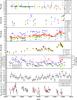 |
Fig. 1 Light curves of Mrk 421 from radio to VHE from 2009 January 19 (MJD 54 850) to 2009 June 1st (MJD 54 983). Vertical bars denote flux measurement errors, and the horizontal bars denote the time bin widths into which some of the light curves are binned. The Fermi-LAT photon fluxes are integrated over a three-day-long time interval. The Whipple 10-m data (with an energy threshold of 400 GeV) were converted into fluxes above 300 GeV using a power-law spectrum with index of 2.5. |
Figure 1 shows the light curves from radio to VHE. No substantial (larger than a factor of 2) flaring activity happened during the campaign; however, some level of variability is present in all energy bands. In the radio band the variability is least pronounced. A significant level of variability is present in the near-infrared (NIR), optical and UV accompanied by an overall increase in flux with time. At X-ray, HE and VHE there is also considerable variability, and only a small overall downward trend in the overall X-ray and VHE flux with time is observed. The X-ray flux variations are stronger on average than the variations in the other wavebands, but still much weaker than the maximum values historically registered for the X-ray and VHE bands (Balokovic et al. 2013; Cortina & Holder 2013).
3.2. Fractional variability
In order to quantify and characterize the variability at different energy bands, we calculated the fractional variability  (1)i.e., the excess variance normalized by the flux, according to Vaughan et al. (2003), where S is the standard deviation of the N flux measurements,
  is the mean squared error and ⟨x⟩2 is the square of the average photon flux. We estimate the uncertainty of Fvar according to Poutanen et al. (2008),
  (2)where
  is given by Eq. (11) in Vaughan et al. (2003):
  (3)This prescription to calculate the uncertainties is more appropriate than Eq. (B2) in Vaughan et al. (2003) for light curves that have an error in the excess variance comparable to or larger than the excess variance. This is, however, not the case for most light curves in our sample, as ΔFvar according to Poutanen et al. (2008) is less than 5% smaller compared to Eq. (B2) in Vaughan et al. (2003). For the Fermi-LAT, and Swift/BAT light curves, the difference is ≈10%.
The Fvar values and errors for the different energy bands (instruments) are shown in Fig. 2. As already noticed when looking at the light curves, Mrk 421 shows little variability in radio, and low but significant variability in all other wavebands with the largest variability in X-rays. We note that in the 2–10 keV band it is intrinsically more variable than in the 0.3–2 keV band, a characteristic which has been recently reported for Mrk 421 during high X-ray and VHE activity (Aleksić et al. 2015b)
Because of the instrument sensitivity, the Fermi-LAT, Swift/ BAT and RXTE/ASM data are binned into 3- and 7-day bins (instead of 1-day bins) and therefore, the variability on smaller timescales is not probed, so Fvar might be underestimated. When rebinning the RXTE/PCA light curve (sampled every ~2 days) into 7-day bins, Fvar decreases by ~15% and agrees with Fvar for RXTE/ASM within the errors. The Swift/XRT light curves are irregularly sampled. There were measurements every ~7 days during the early part of the campaign but there are also large gaps and a period of sub-daily observations. Rebinning the Swift/XRT light curves into 1- and 7-day bins does not change Fvar by more than a few percent and all values agree within the errors.
The results reported in Fig. 2 are not affected by the temporal binning or the uneven sampling of the light curves and hence can be considered as characteristic of Mrk 421 during the multi-wavelength 2009 campaign (see Appendix A for details).
It is interesting to compare these results with the ones reported recently for Mrk 501 in Doert et al. (2013) and Aleksić et al. (2015a), where the fractional variability increases with energy and is largest at VHE, instead of X-rays. The comparison of these observations indicates that there are fundamental differences in the underlying particle populations, environment, and/or processes producing the broadband radiation in these two archetypical VHE blazars. The higher X-ray variability in Mrk 421 might also be related to the higher synchrotron dominance with respect to the one observed in Mrk 501. According to the broadband SEDs measured for Mrk 501 and Mrk 421 during the typical (non-flaring) activity (Abdo et al. 2011b,a),  for Mrk 501 and
  for Mrk 421. These SEDs were parametrized within the one-zone SSC framework in Abdo et al. (2011b,a), using, for Mrk 421, a magnetic field B ~ 2.5 times higher than the one used for Mrk 501 (38 mG vs. 15 mG), which naturally produces a synchrotron bump that is relatively higher than the inverse-Compton bump. The higher magnetic field in Mrk 421 may also lead to a higher variability in the X-ray band (with respect to the γ-ray bump) through a faster synchrotron cooling of the high-energy electrons (τcool − Sync ∝ 1 /B2).
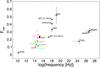 |
Fig. 2 Fractional variability Fvar as a function of frequency. Open circles denote Fvar values in R-band calculated with the host galaxy subtracted as prescribed in Nilsson et al. (2007) |
3.3. Evolution of the X-ray spectral shape with the X-ray flux
Systematic variations of the X-ray spectral shape are a common phenomenon during blazar flares (e.g. Fossati et al. 2000). A harder-when-brighter behavior is quite typical during flares in blazars, and this characteristic has already been observed in Mrk 421 (e.g. Tramacere et al. 2009). Sometimes one can identify loops in the photon index vs. flux diagram during the course of a flare, which could be related to the dynamics of the system, as reported by Kirk & Mastichiadis (1999) or Rieger et al. (2000). Such behavior was also observed in Mrk 421 during a big flare in 1994 (Takahashi et al. 1996). Here we investigate whether these patterns exist in Mrk 421 during its typical (non-flaring) activity.
The Swift/XRT spectrum cannot be fit with a simple power-law because this instrument covers the peak of the synchrotron bump, and hence the X-ray spectrum in the 0.3–10 keV band is curved. We can quantify the hardness of the Swift/XRT spectra by using the ratio of the X-ray fluxes in the bands 2–10 keV and 0.3–2 keV, and study its evolution with respect to the X-ray flux in the 2–10 keV band. This is shown in the left-hand panel of Fig. 3. The RXTE/PCA spectra, which cover the falling segment of the synchrotron bump (when the source is not flaring), can be fit with a simple power-law function, and hence here we can report the spectral slope vs. the X-ray flux in the 2–10 keV band. This is shown in the in the right-hand panel of Fig. 3. Both Swift and RXTE show clearly that the X-ray spectra harden when the X-ray emission increases, and hence we can confirm that the harder-when-brighter behavior also occurs when the source is not flaring. We also investigated the temporal evolution of the plots shown in Fig. 3, looking for loop patterns in the spectral shape-flux plots (clockwise or counter-clockwise) but we did not find any.
3.4. Power density spectrum
Another way to characterize the variability of a given source is the power spectral density (PSD). The PSD quantifies the variability amplitude as a function of Fourier frequency (or timescale) of the variations. The derivation of the PSD is based on the discrete Fourier transform of the light curve under consideration. For blazars, the shape of the PSD is usually a power-law Pν ∝ ν− α with spectral index α between 1 and 2 (Abdo et al. 2010; Chatterjee et al. 2012), i.e., there is larger variability at smaller frequencies/longer timescales. This is generally referred to as “red noise”. Other features in the PSD, such as breaks or peaks, indicate characteristic timescales or (quasi)periodic signals.
Calculating the PSD via the discrete Fourier transform is straightforward for light curves that are frequently and regularly sampled over a long period of time. However, in reality, observation time is usually limited and often interrupted by bad weather, object visibility and technical issues, i.e., we are normally dealing with unevenly sampled light curves of limited length that may have large gaps, and this has serious effects on the measured PSD. If the light curve is discretely sampled instead of continuous (which is usually the case as we are dealing with discrete observations or values that are binned over a certain time period), its Fourier transform is convolved with a windowing function, which becomes very complicated when a light curve has an uneven sampling and gaps (Merrifield & McHardy 1994). In addition, light curves of a finite length are affected by red-noise leak, i.e., variability below the smallest frequency (or largest timescale) probed. This variability power leaks into the observed frequency band and changes the observed PSD shape. This effect can manifest as a rise/fall trend throughout the entire time interval of the light curve. Likewise, aliasing, i.e., variability power from frequencies larger than the Nyquist frequency, affects the variability in the observed frequency range. The effect of sampling on the study of periodicities will be discussed in Sect. 5.
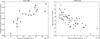 |
Fig. 3 Left: X-ray hardness ratio for the Swift/XRT bands 2–10 keV and 0.3–2 keV vs. the X-ray flux in the 2–10 keV band. Right: power-law index of RXTE/PCA spectra above 3 keV vs. the X-ray flux in the 2–10 keV band. |
These effects of the sampling pattern on the PSD can be avoided by using the simulation-based approach of Uttley et al. (2002; PSRESP) to derive the intrinsic PSD of a light curve and its associated uncertainties. We applied this Monte Carlo fitting technique following the prescription given in the appendix of Chatterjee et al. (2008) to all light curves with ~30 or more flux measurements.
First we generated a large set of simulated light curves using the method of Timmer & Koenig (1995). In order to accommodate the problems introduced by the sampling of the light curve, the simulated light curves were about 100 times longer than the measured light curve and then clipped to the required length. This way, they suffer from red-noise leak in the same way as the measured light curve. The simulated light curves also had a much finer sampling than the measured light curve and were then binned to the required binning to include the aliasing effect. Finally, the simulated light curves were resampled with the observed sampling function, so that the windowing function is the same for the measured and the simulated light curves. Poisson noise was added to each simulated light curve to account for observational noise. As a model for the underlying PSD of the simulated light curves we assumed a power-law shape and varied the power-law index α in the range 1.0 to 2.5 in steps of 0.1. We generated 1000 simulated light curves per α value and per measured light curve. We then calculated the PSD for each measured light curve and the 1000 simulated light curves of each model, taking as the PSD the modulus squared of the mean subtracted light curves’ discrete Fourier transform between the minimum frequency νmin = 1 /T and the Nyquist frequency νNy = N/ 2T. T is the duration of the light curve. The frequency range covered by our data is approximately 10-7 − ≳ 10-5.7 s-1 (corresponding to ≈1/120 days-1 −≈1 / 6 days-1), differing somewhat between the light curves depending on the individual length and binning. The light curves were binned into 2 − 7-day bins, depending on the light curve characteristics. The goodness-of-fit of each PSD model was determined according to the recipe given in the appendix of Chatterjee et al. (2008): The observed χ2 function (4)from the observed PSDobs, the average of the 1000 PSDs from simulated light curves
  , and the standard deviation ΔPSDsim was compared to the simulated χ2 distribution
  (5)calculated from each of the 1000 individual PSDs from simulated light curves PSDsim,i. The success fraction (SuF) is then the fraction of
  larger than
  .
.
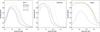 |
Fig. 4 Success fraction as a function of power-law index α of the PSD for three selected light curves (GRT V band, RXTE/PCA and MAGIC) and a range of light curve binnings (2 − 6 days) to illustrate the effect of the binning. The location of the maximum does not change significantly with the binning, but there is significant variation in shape, width and amplitude. |
Figure 4 shows the SuFs for selected measured light curves and Table 1 gives the best-fit power-law indices α and their uncertainties, calculated as the half width at half maximum (HWHM) of the SuF vs. α curve.
We tried a range of binnings and found that the location of the maximum does not vary systematically with the binning (Fig. 4). The uncertainties, however, depend strongly on the light curve binning and on the logarithmic binning of the PSD (Papadakis & Lawrence 1993). We used light curve bin sizes of a few days (between 2 and 6) and a factor of 1.2 or 1.3 by which the logarithmically spaced frequency bins are separated, in order to reduce the scatter in the PSD points. Sometimes the flux measurements have large uncertainties (mean error non-negligible compared to the variance of the light curve as, e.g., in the case of Fermi-LAT) or the light curve has large gaps and/or relatively few data points (e.g., MAGIC). In these cases α is mostly unconstrained. Large gaps or very uneven binning may result in large SuF differences (e.g., MAGIC), or even in changes of the overall shape (e.g., OVRO). In these cases there is no good way to bin the data and obtain a reliable α. If the binning is too small, large gaps are filled with interpolated (probably unrealistic) data in order to calculate the discrete Fourier transform. This results in unwanted changes in the reconstructed PSD and thus in unreliable α values. If the binning is so large that it accomodates also the large gaps such that not too much interpolation is necessary, there are too few data points left and the covered frequency interval becomes too small for a reasonable PSD fit. Unfortunately, the light curves are too short to make analyses based on contiguous parts of a light curve between large gaps.
The maximum of the SuF vs. α curve is generally ≳0.8 for all light curves, but we note that for certain binnings the maximum SuF can be significantly lower, or saturate at 1.0. Thus a power-law seems to be a reasonably good fit for all light curves, but as explained above, the fit is restricted by the limited frequency range and by the light curve sampling or gaps. In Table 1 we give the α values where the SuF has a maximum, i.e., the best-fitting power-law indices. As uncertainties we mention only the median HWHM of the distribution of HWHM from different light curve binnings between 2 and 6 days, but please note that this value itself has an uncertainty. In many cases it is not clear why we should prefer one binning over another, so a certain range in SuF shapes is possible. It should be pointed out that these uncertainties in deriving the width of the SuF vs. α curve do not affect the analysis in the following sections, as we always use the best-fitting α, which does not vary with the binning.
Power spectral density (PSD) index α and half-width at half-maximum of the success fraction (SuF) for light curves with more than 30 flux measurements.
The best-fitting PSD models for most light curves are found to be power-laws with indices ~1.3–1.6. There are no big differences between the SuF vs. α curves of different instruments. The only exceptions are GASP R band and OVRO, where the shape is different and α is higher (though still in agreement with the other α values within the uncertainties). A possible explanation might be the small flux error bars and the dense sampling (several values per night, i.e., larger frequency range compared to all other light curves). Without logarithmic binning and with a light curve binning of 1 or 2 days there is a clear maximum at α = 1.8.
There is no evidence of a break in the (relatively short) frequency range covered by the multi-wavelength data. Simulated light curves with an underlying broken power-law PSD did not improve the success fraction. The X-ray PSD power-law indices are similar to the ones reported in Kataoka et al. (2001) for the same frequency range. The PSD shape and α are consistent with what was found for blazars by other authors (Chatterjee et al. 2008: X-rays; Abdo et al. 2010: HE γ rays).
4. Cross-correlations
We use the discrete cross-correlation function (DCF) method of Edelson & Krolik (1988) to quantify the correlation of the flux variations between all possible light curve pairs, as long as the light curve has more than 30 flux measurements, i.e., we use the same set of light curves as in Sect. 3.4. This way we can assess correlations between VHE, HE γ rays, X-ray, UV, optical and some radio frequencies.
As a cross-check, we calculate for each light curve pair also the z-transformed cross-correlation function (ZDCF; Alexander 1997). The ZDCF is based on the DCF, but the bin widths of the ZDCF are chosen such that the number of points is the same for each bin, i.e., they are different-sized as opposed to the DCF, where all bins have the same size. In addition, Fisher’s z-transform is applied to the cross-correlation coefficients. According to Larsson (2012), the ZDCF is more robust than the DCF for undersampled (w.r.t. the flux variations) light curves. However, for well sampled light curves, the ZDCF has been shown to be consistent with the DCF (e.g., Dietrich et al. 1998; Smith & Vaughan 2007). For this study we used mostly the DCF, as the temporal bin is fixed, so that it also allows us to trivially compare and even combine results from different pairs of instruments. Therefore, we used the ZDCF for verification purposes only.
Two different approaches are used to determine the uncertainties of the DCF. The easiest and fastest way is to simply use the errors given in Edelson & Krolik (1988). However, as discussed in Uttley et al. (2003), these are not appropriate for determining the significance of the DCF when the individual light curve data points are correlated red-noise data. Depending on the PSD and the sampling pattern, the significance as calculated by Edelson & Krolik (1988) might be overestimated. To get a better estimate on the real significance of the correlation peaks we used a Monte Carlo approach, following the descripion of Arévalo et al. (2009). The Monte Carlo technique is described in detail in Sect. 4.1.
We used a binning of six days for all DCFs because this way different DCFs can be easily compared or, if needed, combined. To make sure that we do not miss correlations or time lags, we always tried a range of binnings, depending on the sampling of the involved light curves.
As the following paragraphs will show, significant correlations are only found between X-rays and VHE. In addition, X-rays and optical light curves seem to follow opposite trends.
4.1. VHE – X-rays
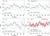 |
Fig. 5 DCF of the combined Whipple and MAGIC (VHE) light curve, correlated with the RXTE/PCA and the Swift/XRT (2–10 keV) light curves are shown in the upper left and lower left panels. The black error bars represent the uncertainties as derived from Edelson & Krolik (1988). The green lines represent the 1% and 99% extremes of the DCF distribution of simulated RXTE/PCA light curves when correlated with the measured VHE light curve. The blue lines represent the 5% and 95% extremes. Upper right panel: average of the VHE–RXTE/PCA and VHE–Swift/XRT (2–10 keV) DCFs, with the corresponding confidence intervals derived from averaging the DCFs of the simulated light curves. See text for details in the calculation of the average DCFs and contours. Lower right panel: z-transformed DCFs. |
The correlation of the flux variations between the VHE (MAGIC, Whipple) and X-ray (RXTE/PCA and Swift/XRT 2–10 keV) bands is shown in Fig. 5. The correlations peak at time lag Δt = 0 and appear to be strongly significant (>5σ), when considering only the errors calculated according to Edelson & Krolik (1988; black error bars). However, as mentioned above, the error bars calculated using Edelson & Krolik (1988) can overestimate the real significance of the correlation. To get a better estimate on the real significance of the correlation peaks we use the following Monte Carlo approach.
For each X-ray light curve we created a set of 1000 simulated light curves in the same way as in Sect. 3.4, using a power-law with the best-fitting slope as determined in Sect. 3.4 from the PSRESP method (see Table 1). The X-ray flux was sampled more often and with smaller statistical errors than the VHE flux, and hence, in order to ascertain the confidence levels in the DCF calculation, it is reasonable to use simulated RXTE/PCA and Swift/XRT (2 − 10 keV) light curves instead of the VHE light curves. We cross-correlated each of the 1000 simulated X-ray light curves with the observed MAGIC and Whipple light curves. A power-law spectrum with index 2.5 (Hillas et al. 1998) was used to normalize the integral flux of the Whipple 10 m data (with an energy threshold of ~400 GeV) to an integral flux above 300 GeV in order to provide a comparison with MAGIC. We therefore also cross-correlated the original and the simulated X-ray light curves with the combined Whipple+MAGIC light curve. From the distribution of 1000 DCFs (i.e., the cross-correlations of the simulated X-ray light curves with the real VHE light curves) we then calculated the 95 and 99% confidence limits, and show them in Fig. 5. For each combination of RXTE/PCA and Swift/XRT (2–10 keV) with MAGIC, Whipple and Whipple+MAGIC the DCF shows a peak at time lag Δt = 0 with a probability larger than 99%. There are no other peaks or dips in the DCF between VHE and X-rays that appear significant. A positive correlation between X-rays and VHE has been reported many times during flaring activity (e.g., Fossati et al. 2008), but has never been observed for Mrk 421 in a non-flaring state. Our simulations show that the real significance of the correlation is 3 − 4σ, indeed confirming that the error bars calculated using Edelson & Krolik (1988) slightly overestimate the significance of the correlation.
We average the DCFs, which has the advantage that spurious features are smoothed out while features present in all DCFs (i.e., those features that are real) are strengthened. This is particularly useful when having many possible combinations and/or marginally significant features like the ones that will be reported in Sect. 4.3. The DCFs were averaged in the following way: for a number of q + 1 real light curves A, B1, ..., Bq we first calculate all q correlation functions DCF(AB1), ..., DCF(ABq) using a binning of 6 days. Then we calculate the average DCF  (6)There is no prescription to combine the uncertainties derived from Edelson & Krolik (1988) for several DCFs, thus no error bars are shown in the upper right panel of Fig. 5. For the determination of the averaged confidence limits we correlate the simulated light curves a1, ..., an or
  , ...,
  (n = 1000,
  ) with the original light curve
  or A using either
  (7)or
(7)or 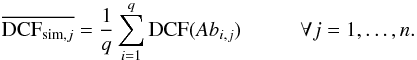 (8)From this distribution of n averaged correlation functions
  we then compute the 95 and 99% confidence limits. Whether we use Eqs. (7) or (8) depends on the sampling of the light curves. The sampling and statistical uncertainties of the X-ray light curves are much better than the sampling of the VHE light curves. Therefore the PSD could be better constrained in the X-ray case and hence the confidence limits obtained from correlating the original VHE with simulated X-ray light curves are more reliable than the confidence limits obtained from correlating the original X-ray with simulated VHE light curves. Thus here the light curve A is Whipple+MAGIC, the light curves Bi are RXTE/PCA and Swift/XRT (2–10 keV) and we use Eq. (8).
The upper right panel of Fig. 5 shows the DCF averaged over the two combinations Whipple+MAGIC – RXTE/PCA and Whipple+MAGIC – Swift/XRT (2–10 keV) and the corresponding confidence limits. There is a clear correlation at time lag Δt = 0 with a high confidence >99%.
The ZDCFs between the VHE and the X-ray light curves show the same behavior as the corresponding DCFs. However, as the binning is different for each ZDCF (ranging from sub-day scales around time lags Δt ≈ 0 days to a few days at time lags Δt ≈ 60 days), it is not possible to combine them as we did with the DCFs. Rebinning the ZDCFs to even 6-day bins, averaging them subsequently and using the simulated light curves to assess the uncertainties yields almost identical results to the averaged DCF.
Both VHE and X-ray light curves show a weak negative trend with time. To make sure that this trend is not responsible for the correlation, we calculated the (z)DCFs also for the detrended light curves. The difference is marginal. In addition, when comparing X-ray and VHE light curves, one can see that the light curve features nicely agree, i.e., the long-term trend has only a minor contribution to the correlation peak, which is driven by shorter timescale variability.
Figure 6 shows the DCF of the combined Whipple and MAGIC light curve, correlated with the Swift/XRT (0.3–2 keV) light curve. Although the DCF has a peak at time lag Δt ≈ 0 days which seems to be significant with a confidence level of around 5σ when considering the Edelson & Krolik (1988) errors, the simulations show that this level of correlation is not significant (only ≈1.5σ).
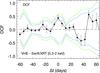 |
Fig. 6 DCF of the combined Whipple and MAGIC (“VHE”) light curve, correlated with the Swift/XRT (0.3–2 keV) light curve. The black error bars represent the uncertainties as derived from Edelson & Krolik (1988). The green lines represent the 1% and 99% extremes of the DCF distribution of simulated Swift/XRT light curves when correlated with the measured VHE light curve. The blue lines represent the 5% and 95% extremes. |
4.2. HE γ rays – UV/optical
Figure 7 shows the combined DCF of the Fermi-LAT light curve, correlated with optical and UV light curves (using simulated optical and UV light curves to estimate the uncertainties)4. There is a peak in the DCF at a time lag Δt = 0 days, but it is not significant. The uncombined DCFs also show a small peak with a significance <3σ or no peak at all when using the Edelson & Krolik (1988) uncertainties. The significance of the small peaks is even lower (<2σ) when using the uncertainties from simulated data. Larger light curve binsizes would reduce the errors, but also lead to significantly fewer data points, a reduced PSD frequency range, and increased DCF bin sizes. Given the small time window (4.5 month long campaign) under consideration, we cannot improve the DCF quality by rebinning.
 |
Fig. 7 Average DCF of the Fermi-LAT HE γ-ray light curve, correlated with the optical and UV light curves (GASP R-band, GRT BVRI, MITSuME g, MITSuME Ic and UVOT W1), shown in black. The green lines represent the 1% and 99% extremes of the likewise averaged DCF distribution of simulated optical/UV light curves when correlated with the real Fermi-LAT light curve. The blue lines represent the 5% and 95% extremes. |
4.3. X-rays – UV/optical
We also searched for correlations between the X-ray and UV/optical bands. As done in the previous subsections, we calculated the DCFs for all possible combinations between RXTE/PCA and Swift/XRT with Swift/UVOT, GASP R band, GRT BVRI, MITSuME g and MITSuME Ic. The results are shown in panel A of Fig. 8. One feature that is common in almost all DCFs is an anti-correlation at a time lag Δt ≈ −20 to −10 days, i.e., optical/UV variations lead X-ray variations by ~15 days. This feature is significant above 99% and is confirmed by the ZDCF. However, it is not immediately clear what might cause this anti-correlation. The first thing that becomes apparent when looking at the light curves is the long-term trend. The UV/optical light curves show a strong positive trend, while the X-ray light curves show a slight negative trend. Therefore it is not surprising that the DCFs show an overall anti-correlation spread over a large range of time lags. However, this characteristic cannot explain the above-mentioned (anti-)correlations with time lags of 10−20 days.
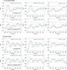 |
Fig. 8 a) DCFs of each X-ray light curve (Swift/XRT (0.3–2 keV), Swift/XRT (2–10 keV) and RXTE/PCA (2–10 keV)), correlated with several optical and UV light curves, are averaged over all optical to UV bands and shown in black in the upper panel. The green lines represent the 1% and 99% extremes of the likewise averaged DCF distribution of simulated optical/UV light curves when correlated with the observed X-ray light curve. The blue lines represent the 5% and 95% extremes. Lower panel: z-transformed DCFs, which were, for the purpose of direct comparison with the DCF, rebinned to the same binning as the DCFs and averaged in the same way. b) Same as a), but all light curves have been detrended (as described in 4.3) before correlation. |
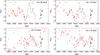 |
Fig. 9 Example plots to illustrate the correlation between the optical and the X-ray flux variations. All four panels show the normalized Swift/XRT (0.3–2 keV) light curve in black. The GASP R-band light curve, normalized and rescaled to match the same flux range as the Swift/XRT light curve, is overplotted in red with different time lags Δt = − 36, −18, + 6, and + 18 days. In case of anti-correlation (Δt = − 18 and + 18 days), the GASP light curve is also flipped vertically. |
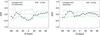 |
Fig. 10 Average of the DCFs of the combined Whipple and MAGIC (VHE) light curve, correlated with several optical and UV light curves, are shown in black in the left panel. The green lines represent the 1% and 99% extremes of the likewise averaged DCF distribution of simulated optical/UV light curves when correlated with the observed VHE light curve. The blue lines represent the 5% and 95% extremes. Right panel: same as the left panel, but all light curves have been detrended (i.e., fitted and subtracted by a first-order polynomial) before correlation. |
Hence we detrended the light curves by fitting and subtracting a first-order polynomial to each light curve and re-calculated the DCFs and the ZDCFs. They are shown in panel B of Fig. 8 in comparison to the correlations of the original light curves (panel A). In the detrended light curves we find two results: 1) the overall negative correlation spread over most time lags disappears. 2) Some peaks become evident at time lags Δt ≈ − 36, −18, + 6 and + 18 days (the latter two being absent in the RXTE/PCA – UV/optical DCF). In the ZDCFs these features are generally less pronounced. The presence of such features leads to the suspicion that an underlying quasi-periodic behavior may be responsible for the (anti-)correlations. Indeed there are several local peaks and minima in both the X-ray and UV/optical light curves. In Fig. 9 we illustrate how well these features correlate by overplotting two light curves (Swift/XRT (0.3–2 keV) and GASP R band). Both light curves are normalized. The GASP light curve is also rescaled such that both light curves cover approximately the same normalized flux range. In addition, the GASP light curve is shifted in x direction by −36, −18, 6 and 18 days. For time lags where an anti-correlation was detected (−18 and + 18 days), we also flipped the GASP light curve about the horizontal axis (such that light curve peaks become troughs and vice versa), such that in each panel of Fig. 9 we should see that both light curves follow the same path whenever there is a real (anti-correlation) present. However, it is obvious from these plots that some, but not all of these features are loosely correlated (as indicated by the low statistical significance of the DCF peaks) and that the limited time window hampers the ability to detect a convincing correlation. The behavior illustrated in Fig. 9 may well happen just by chance without being caused by an underlying physical mechanism. In Sect. 5 we show that there is no hint of a periodic signal in any of the light curves.
4.4. VHE – optical/UV
The VHE light curves, when correlated with UV and optical light curves, produce a strong negative peak at time lag Δt = 0 days (Fig. 10), i.e., they are anti-correlated with a probability larger than 99%. However, the optical/UV light curves show a strong positive trend while the VHE light curves show a weak negative trend. After detrending the light curves, the anti-correlation at time lag Δt = 0 days disappears. Instead, the DCF now shows a similar behavior as the X-ray–optical DCFs (marginally significant anti-correlation at time-lag Δt ≈ − 18 days and correlation at ≈−36 days). This is not surprising given the positive correlation between VHE and X-ray fluxes. More data in the typical state are needed in order to judge whether this behavior is just a chance (anti-)correlation or if it is caused by underlying physical mechanisms.
4.5. Other correlations
All the data in the optical and UV bands vary simultaneously as shown in Fig. 1. The NIR bands seem to be well correlated with the optical and UV bands. However, the number of flux measurements per NIR light curve is too small to calculate a meaningful DCF or ZDCF.
No significant correlations are found between radio or HE γ rays with other wavelengths.
5. Periodicities
5.1. Lomb-Scargle periodogram
Although the Lomb-Scargle periodogram (LSP) is not the best way to determine the PSD for red-noise data (Kastendieck et al. 2011), it is a good way to find periodicities when dealing with unevenly sampled light curves.
A peak in the LSP at a certain time lag can mean that there is a periodicity. However, the sampling also produces peaks, e.g., if there is a flux measurement every 2 days, there will be a strong peak at period P = 2 days. Uneven sampling may result in one or more peaks, if at least part of the flux measurements follow an approximately regular observation schedule. The LSPs were determined for periods ≤L/ 5 ≈ 25 days, where L is the length of the light curve. To estimate the significance of potential LSP peaks, we also calculated the LSP for 1000 simulated light curves each. The simulated light curves were produced in the same way as in Sect. 3.4 and have the same underlying PSD (estimated above with PSRESP) and the same sampling as the original light curve. From the distribution of LSPs we determined the 95% and 99% confidence limits. We did not find significant LSP peaks in any of the light curves. A peak around P ≈ 18 days is present in a few optical and X-ray LSPs, but always below 99% confidence level, and in most LSPs even below 95% confidence level.
5.2. Autocorrelation
We use the discrete correlation function (Edelson & Krolik 1988) to calculate the discrete auto-correlation function (DACF) of the variability of Mrk 421 in all observed wave bands. Equally spaced and repeated features in the DACF might be a hint to characteristic timescales and quasi-periodicities. As in the previous sections, we use simulated light curves to estimate the significance of DACF peaks, i.e., the observed light curve is correlated with 1000 simulated light curves. This results in confidence limits that are not symmetric around zero, although the DACF itself is symmetric. The origin of the asymmetry relies on the process used to determine the confidence intervals, which uses 1000 Monte Carlo realizations of one light curve, together with the asymmetry of some of the light curves. This results in different Monte Carlo realizations when the light curve is truncated on the left or on the right (negative or positive time lags), hence yielding different results for the confidence intervals. Consequently, the asymmetry in the confidence intervals is particularly strong where the sampling and variability of the light curve changes significantly with time (e.g., UVOT). Figure 11 shows DACFs for a few representative light curves. There are secondary peaks in some DACFs. However, they are all well below the 95% limit, i.e., they do not appear to be significant. Hence we do not find significant periodicities or characteristic timescales.
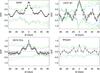 |
Fig. 11 Discrete auto-correlation function for a few light curves are shown in black. The green lines represent the 1% and 99% extremes of the likewise averaged DACF distribution of simulated light curves when correlated with themselves. The blue lines represent the 5% and 95% extremes. |
6. Discussion of the main observational results
Even though Mrk 421 is known for extreme X-ray and VHE variability, with short and intense flares (e.g. Gaidos et al. 1996; Fossati et al. 2008; Aleksić et al. 2012), the X-ray and VHE activity measured in the 2009 observing campaign was relatively mild, with X-ray/VHE flux variations typically smaller than a factor of 2. The VHE flux of Mrk 421 was also relatively low, with an average flux of about 0.5 times the flux of the Crab Nebula, which is typical for this source (Acciari et al. 2014). Regardless of the low activity, Mrk 421 showed significant variability in the portions of the electromagnetic spectrum where it emits most of its energy power, namely optical/UV, X-rays and HE/VHE γ rays. The optical/X-ray bands bring information from the rising/falling segments of the low-energy bump, while the HE/VHE bands tell us about the rising/falling segment of the high-energy bump. As reported in Sect. 3.2 (see Fig. 2), the highest variability occurs at X-rays (Fvar ~ 0.5), then VHE (Fvar ~ 0.3), and then optical/UV/HE (Fvar ~ 0.2). It is interesting to compare these results with the ones reported recently for Mrk 501 (Doert et al. 2013; Aleksić et al. 2015a), where the fractional variability increases with energy and is largest at VHE, instead of X-rays. The comparison of these two observations indicates that there are fundamental differences in the underlying particle populations and/or processes producing the broadband radiation in these two archetypical VHE blazars. Within the one-zone synchrotron self-Compton scenario, which is commonly used to model the emission of VHE blazars, the X-ray and VHE variability is driven by the dynamics of the population of relativistic electrons through their synchrotron and inverse-Compton emission, respectively. Within this scenario, and for typical model parameters, the ~keV emission is dominated by higher-energy electrons, whereas the ~100 GeV emission is produced by a mixture of lower-energy electrons that inverse-Compton scatter in Thomson regime, and high-energy electrons that inverse-Compton scatter in Klein-Nishina regime (see Paper I). Consequently, the multi-band fractional variability reported in Sect. 3.2 indicates that the population of higher-energy electrons varies more than that at lower energies.
It is worth noticing that the fractional variabilities detected in the energy range 2–10 keV measured by RXTE/PCA, RXTE/ASM and Swift/XRT agree reasonably well with a value of 0.4–0.55 despite the different observing windows of these three different instruments. On the other hand, the fractional variability measured by Swift/XRT in the energy range 0.3–2 keV is ~0.25, which is a factor of 2 lower than the variability detected by Swift/XRT in the 2–10 keV energy range. Given that these two observations are performed with the same instrument, the difference in the fractional variability cannot be ascribed to a different observing temporal period that might include or exclude a particular flux variation, and hence the higher variability in the 2–10 keV energy range, in comparison to that in the 0.3–2 keV energy range, is an intrinsic property of Mrk 421 during the 2009 observing campaign, which has also been recently reported for Mrk 421 during high X-ray and VHE activity observed in 2010 (Aleksić et al. 2015b). Because the characteristic synchrotron frequency of relativistic electrons is proportional to the square of the energy of the electrons ( ), the higher synchrotron energies will be produced by higher energy electrons, and hence this further supports the theoretical framework of higher variability in the number of higher energy electrons. Given that the high energy electrons are the ones losing their energy fastest (
 ), in order to keep the source emitting X-rays, injection (acceleration) of electrons up to the highest energies is needed. We therefore conclude that the injection (acceleration) of high-energy electrons is likely to be the origin of the flux variations in Mrk 421.
From the multi-instrument light curves shown in Fig. 1, it can be seen that, while the variability in X-ray and VHE occurs mostly on ~day timescales, the variability at optical/UV occurs mostly on ~week or even longer timescales6. The different variability timescales do not show up in the results reported in Sect. 3.4 (see Table 1). However, this might be the result of the limited sensitivity of the PSD analysis due to the uneven sampling of the light curves, and the rather small range of frequencies sampled (10-7 −≈10-5.7 s-1), which do not provide a long enough lever arm to determine accurately (and ultimately to distinguish) the index of the power-law spectrum of the PSDs from the different energy bands. Therefore, the multi-band light curves and fractional variability show similarities in the X-ray and VHE flux variations, which differ from characteristics of the optical/UV flux variations. This observation is further confirmed by the cross-correlation results reported in Sect. 4, which show a positive correlation with no time lag between the X-ray and VHE emission, but not between the optical/UV and X-ray or VHE. This result indicates that both the X-ray and VHE emissions are co-spatial and produced by the same population of high-energy particles. It is worth noting that, while such a correlation has been reported many times for Mrk 421 during flaring activity (e.g. Fossati et al. 2008), this is the first time that this is observed during a non-flaring (typical) state. Therefore, together with the observed harder-when-brighter behavior in the X-ray spectra, we interpret this experimental observation as evidence that the mechanisms responsible for the X-ray/VHE emission during non-flaring-activity states might not differ substantially from the ones responsible for the emission during flaring-activity states. In particular, the positive X-ray/VHE correlation observed during flaring activity in Mrk 421 and many other blazars has been interpreted by many authors as evidence for leptonic scenarios, and hence against the hadronic scenarios where the X-ray emission and the γ-ray emission are produced by different particle populations and processes. However, with a fine tuning of the parameters, hadronic models are also able to explain single flaring events with an X-ray/VHE correlation with time lag zero (Mastichiadis et al. 2013).
The observations presented here confirm that the relation between X-ray and VHE bands also exists when the source is not flaring. That is, such a relation is persistent over long timescales of at least several months, and does not occur only on single flaring events, and that is much more difficult to explain with hadronic scenarios. Therefore, these observations provide strong evidence supporting leptonic scenarios as responsible for the dominant X-ray/VHE emission from Mrk 421.
Another result that is worth discussing is the overall anti-correlation between the X-ray and optical bands. This anti-correlation spreads over a large range of time lags and hence it is fundamentally different from the one obtained for the X-ray and VHE bands. As we show in Sect. 4, the origin of this overall anti-correlation is the long-term trends of the optical/UV and X-ray activity: while the former increases over time during the observing campaign, the latter decreases. The temporal evolution of the optical and X-ray/VHE bands is complex, and a dedicated correlation analysis over many years will be necessary in order to properly characterize it.
For the 2009 multi-wavelength campaign, we do observe an anti-correlation in the (long-term) temporal evolution between optical/UV and X-rays, and hence it is worth discussing possible theoretical scenarios that might lead to this situation. The first scenario is that the optical/UV and the X-ray/VHE emissions are dominated by the emission from two distinct and unconnected regions with different temporal evolutions of their respective particle populations. In such case, the optical/UV vs. X-ray anti-correlation observed in the 2009 multi-instrument campaign would have occurred by chance, and hence we would also expect to see multi-month time intervals with a positive correlation, or no correlation. A second scenario would be a two-component (high- and low-energy) particle population, in which the low- and high-energy particles have a different but related long-term temporal evolution. A change in the magnetic field intensity while keeping the acceleration timescale constant could lead to the observed optical/UV–X-ray (long-term) anti-correlation. An increase in the magnetization would produce a higher synchrotron emission with a decrease in the energy of the electrons (due to a stronger cooling), which effectively would lead to a higher optical emission with a lower X-ray emission. On the other hand, a lower magnetization would lead to a decrease in the total emitted synchrotron flux, but a higher maximum electron energy, which effectively could lower the optical flux and increase the X-ray flux. In practice, such a scenario would be somewhat similar to the blazar sequence (Ghisellini et al. 1998), with the difference that in the latter scenario the different coolings would relate to different sources instead of different states of the same source. A third scenario could be a global long-term change in the efficiency of the acceleration mechanism that produces the electron energy distribution. Such a change in the global efficiency could shift the entire synchrotron bump to higher/lower energies. For instance, if the acceleration mechanism becomes more efficient to get electrons up to the highest energies at the expense of keeping a lower number of low-energy electrons (i.e., the index of the electron population gets harder), the emission at the rising segment of the synchrotron bump (optical) would decrease, while that on the decreasing segment of the synchrotron bump (X-rays) would increase.
In this study we did not see any correlation between the radio fluxes and those at higher frequencies. However, since the measured radio emission is expected to have large contributions from regions farther away in the jet, it is not surprising to see a non-correlation between radio and optical, X-ray and/or γ-ray energies on timescales of days to weeks. We note, however, that such correlation might be apparent during large flares when the radio emission might be strongly dominated by the same region responsible for the overall broadband emission.
7. Conclusions
We studied the broadband evolution of the SED of Mrk 421 through a 4.5 month long multi-instrument observing campaign in 2009, when the source was in its typical (non-flaring) activity state, with a VHE flux of about half that of the Crab Nebula. Even though the source did not show flaring activity, we could measure significant variability in the energy bands where the emitted power is largest: optical, X-ray, γ rays and VHE. The highest variability occurred in the X-ray band, which, within the standard one-zone SSC scenario, indicates that the high-energy electrons are more variable than the low-energy electrons. We also observed a harder-when-brighter behavior in the X-ray spectra, and found a positive correlation between the X-ray and VHE bands. In the literature one can find many works reporting a positive correlation between the X-ray and VHE fluxes (e.g. Fossati et al. 2008, and references therein) and spectral shape changes with the X-ray flux (e.g. Tramacere et al. 2009), but only when Mrk 421 was showing VHE flaring activity (i.e., VHE flux above the flux of the Crab Nebula). This is the first time that such characteristics are reported for non-flaring activity and suggests that the processess occurring during the flaring activity also occur when the source is in a non-flaring (low) state. In particular, this is a strong argument in favor of leptonic scenarios dominating the broadband emission of Mrk 421 during non-flaring activity, since such a temporally extended X-ray/VHE correlation cannot be explained within the standard hadronic scenarios. Moreover, a negative correlation in the (long-term) temporal evolution of the optical/UV and X-ray bands was also observed. Such a trend could be produced in a region with a particle population where the low- and high-energy particles evolve differently but in a related way, which could be produced by a change in the magnetization of the region while keeping the acceleration timescales constant, or by a global change in the efficiency of the mechanism accelerating the electrons. In any case, even though statistically significant for the 2009 multi-instrument campaign, the current dataset does not allow us to exclude that this optical/X-ray anti-correlation was observed by chance, and hence that the optical and the X-ray bands are produced by distinct and unrelated particle populations that evolve separately. Further multi-instrument observations extending over many years will help to address this question.
Online material
Appendix A: Reliability of Fvar
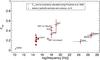 |
Fig. A.1 Measured fractional variability Fvar (black) compared with a delete-d jackknife estimate (red) with |
Almost all light curves of the campaign are unevenly sampled. The sampling is different for each instrument depending on observation schedule, weather and technical issues. There are often gaps of different lengths in the light curves and each light curve has a different number of data points ranging from a few up to a few hundred. In addition, some light curves are binned into bins of several days because of the limited sensitivity of the corresponding instruments. Therefore we have to assess whether there is an error introduced to Fvar by the uneven sampling and the binning and how the Fvar values can be compared. In addition we need to know the minimum number of flux measurements per light curve which are needed to obtain a reliable, unbiased Fvar value.
To address these questions, we first made a delete-d jackknife analysis, i.e., from each light curve containing N data points, we randomly removed d data points (1 ≤ d ≤ N − 2) and calculated Fvar for this reduced sample of N − d data points. Applying a delete-d jackknife analysis on a time series is formally not correct, as the data are correlated in time (blazar light curves usually show a red-noise behavior). However, our purpose is to create datasets that have statistical properties
identical to the real data to demonstrate the impact of gaps and uneven sampling on Fvar. Figure A.1 shows Fvar for the jackknife datasets with  in comparison with Fvar for the original light curves. The Fvar values do not change significantly. The error bars are larger because of the reduced number of flux values in the jackknife samples. The result does not depend on the particular choice of d, as long as there are sufficient datapoints in the jackknife-samples remaining. Some of the light curves are (almost) regularly sampled, namely Fermi-LAT, RXTE/PCA and RXTE/ASM. These are good examples that demonstrate that irregular sampling does not introduce a bias to the Fvar measurement.
We also varied d between 1 and N − 2. Figure A.2 shows Fvar vs. (N − d) /N for selected light curves. As long as N − d is larger than ~5, the measured Fvar is approximately constant with varying d and in agreement with Fvar of the original light curve. Likewise, the error bars do not change significantly. Strong deviations from Fvar of the original light curve occur only, if at all, when N − d< 10. No significant deviations are observed at N − d ≥ 20 for any of the light curves. Thus we conclude that our Fvar measurement is robust for all light curves with 20 or more flux data points. In our multi-wavelength sample most light curves in the optical, UV, X-rays, HE γ rays and VHE have more than 20 flux data points. In the radio and near-infrared, most light curves do not.
Fvar is reliable for all but the smallest samples. If after removal of d data points the remaining sample is smaller than about 10, then Fvar might be over- or underestimated.
We also made a moving-block jackknife test, i.e., we removed blocks of m consecutive measurements. This test is still formally correct when the data are slightly correlated in time, but the drawback is that the number of jackknife samples is much smaller than in case of the delete-d jackknife test. Likewise, it only shows the influence of gaps, not the influence of a random sampling. Figure A.3 shows the test for ![Mathematical equation: \hbox{$m=\sqrt[3]{N}$}](/articles/aa/full_html/2015/04/aa24216-14/aa24216-14-eq143.png) . As in the case of the delete-d jackknife test, the Fvar values do not change significantly and the uncertainties are larger.
. As in the case of the delete-d jackknife test, the Fvar values do not change significantly and the uncertainties are larger.
These conclusions, however, are only valid because the dataset does not have any strong flare and hence it is unaffected by removing points or blocks randomly. Occasional strong flares therefore should be removed before doing an Fvar analysis of light curves that are otherwise in a typical or low state.
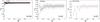 |
Fig. A.2 Fractional variability Fvar (red) as a function of (N − d) /N for the jackknife-d samples of selected representative light curves. The measured Fvar of the original light curve and its error are shown as red horizontal lines. The Fvar of the jackknife-samples is constant and agrees with the original Fvar within its errors for all but the largest d (i.e., the smallest jackknife-samples). |
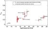 |
Fig. A.3 Measured fractional variability Fvar (black) compared with a moving-block jackknife estimate (red), using a blocksize of |
We use the term “typical” instead of “quiescent”, to describe a state that is neither exceptionally high/flaring, nor at the lowest possible level. Even though the term “quiescent” has been used in the past to denote non-flaring activity in Mrk 421 and other blazars, we note that the term quiescent refers to the lowest possible emission, which is actually unknown, and hence not suitable in this context.
E.g., for imaging air Cherenkov telescopes (IACTs) like MAGIC or Whipple, observations during moonlight are only possible to a very limited extent, resulting in regular gaps of ~10 days in the VHE light curves.
In Sect. 3.4 we showed that it is not possible to constrain the PSD of the Fermi-LAT light curve because of the large error bars of the light curve data points.
As discussed in Sect. 3.2, the somewhat lower value of RXTE/ASM, 0.33+/−0.03, is due to the 7-day integration time, which prevents the detection of variability with temporal scales of days.
Because of the 3-day span and the relatively large statistical uncertainty in the flux points, we cannot evaluate whether short or long timescales dominate the variability in the HE γ-ray band.
Acknowledgments
We would like to thank the referee for the useful comments that helped to improve the manuscript. We also thank Patricia Arévalo for helpful contributions and suggestions. The MAGIC collaboration would like to thank the Instituto de Astrofísica de Canarias for the excellent working conditions at the Observatorio del Roque de los Muchachos in La Palma. The financial support of the German BMBF and MPG, the Italian INFN and INAF, the Swiss National Fund SNF, the ERDF under the Spanish MINECO, and the Japanese JSPS and MEXT is gratefully acknowledged. This work was also supported by the Centro de Excelencia Severo Ochoa SEV-2012-0234, CPAN CSD2007-00042, and MultiDark CSD2009-00064 projects of the Spanish Consolider-Ingenio 2010 programme, by grant 268740 of the Academy of Finland, by the Croatian Science Foundation (HrZZ) Project 09/176 and the University of Rijeka Project 13.12.1.3.02, by the DFG Collaborative Research Centers SFB823/C4 and SFB876/C3, and by the Polish MNiSzW grant 745/N-HESS-MAGIC/2010/0. The VERITAS collaboration acknowledges support from the US Department of Energy, the US National Science Foundation and the Smithsonian Institution, by NSERC in Canada, by Science Foundation Ireland, and by STCF in the UK. We acknowledge the excellent work of the technical support at the FLWO and the collaboration institutions in the construction and operation of the instrument. The Fermi-LAT Collaboration acknowledges support from a number of agencies and institutes for both development and the operation of the LAT as well as scientific data analysis. These include NASA and DOE in the United States, CEA/Irfu and IN2P3/CNRS in France, ASI and INFN in Italy, MEXT, KEK, and JAXA in Japan, and the K. A. Wallenberg Foundation, the Swedish Research Council and the National Space Board in Sweden. Additional support from INAF in Italy and CNES in France for science analysis during the operations phase is also gratefully acknowledged. We acknowledge the use of public data from the Swift and RXTE data archives. The OVRO 40 m monitoring program is supported in part by NASA grants NNX08AW31G and NNX11A043G, and NSF grants AST-0808050 and AST-1109911. The Metsähovi team acknowledges the support from the Academy of Finland to our observing projects (numbers 212656, 210338, 121148, and others). The Abastumani Observatory team acknowledges financial support by the Shota Rustaveli National Science Foundation through project FR/577/6-320/13. The St. Petersburg University team acknowledges support from the Russian RFBR foundation via grant 09-02-00092. AZT-24 observations are made within an agreement between Pulkovo, Rome and Teramo observatories. This research is partly based on observations with the 100 m telescope of the MPIfR (Max-Planck-Institut fuer Radioastronomie) at Effelsberg, as well as with the Medicina and Noto telescopes operated by INAF–Istituto di Radioastronomia. M. Villata organized the optical-to-radio observations by GASP-WEBT as the president of the collaboration.
References
- Abdo, A. A., Ackermann, M., Ajello, M., et al. 2010, ApJ, 722, 520 [NASA ADS] [CrossRef] [Google Scholar]
- Abdo, A. A., Ackermann, M., Ajello, M., et al. 2011a, ApJ, 727, 129 [NASA ADS] [CrossRef] [Google Scholar]
- Abdo, A. A., Ackermann, M., Ajello, M., et al. 2011b, ApJ, 736, 131 [NASA ADS] [CrossRef] [Google Scholar]
- Acciari, V. A., Arlen, T., Aune, T., et al. 2014, Astropart. Phys., 54, 1 [NASA ADS] [CrossRef] [Google Scholar]
- Albert, J., Aliu, E., Anderhub, H., et al. 2007, ApJ, 663, 125 [NASA ADS] [CrossRef] [Google Scholar]
- Aleksić, J., Alvarez, E. A., Antonelli, L. A., et al. 2012, A&A, 542, A100 [NASA ADS] [CrossRef] [EDP Sciences] [Google Scholar]
- Aleksić, J., Ansoldi, S., Antonelli, L. A., et al. 2015a, A&A, 573, A50 [NASA ADS] [CrossRef] [EDP Sciences] [Google Scholar]
- Aleksić, J., Ansoldi, S., Antonelli, L. A., et al. 2015b, A&A, in press, DOI: 10.1051/0004-6361/201424811 [Google Scholar]
- Alexander, T. 1997, in Astronomical Time Series, eds. D. Maoz, A. Sternberg, & E. M. Leibowitz, Astrophys. Space Sci. Lib., 218, 163 [Google Scholar]
- Arévalo, P., Uttley, P., Lira, P., et al. 2009, MNRAS, 397, 2004 [NASA ADS] [CrossRef] [Google Scholar]
- Balokovic, M., Furniss, A., Madejski, G., & Harrison, F. 2013, ATel, 4974, 1 [NASA ADS] [Google Scholar]
- Chatterjee, R., Jorstad, S. G., Marscher, A. P., et al. 2008, ApJ, 689, 79 [NASA ADS] [CrossRef] [Google Scholar]
- Chatterjee, R., Bailyn, C. D., Bonning, E. W., et al. 2012, ApJ, 749, 191 [NASA ADS] [CrossRef] [Google Scholar]
- Cortina, J., & Holder, J. 2013, ATel, 4976, 1 [NASA ADS] [Google Scholar]
- Dietrich, M., Peterson, B. M., Albrecht, P., et al. 1998, ApJS, 115, 185 [NASA ADS] [CrossRef] [Google Scholar]
- Doert, M., David Paneque for the MAGIC Collaboration, the VERITAS Collaboration, & the Fermi-LAT Collaboration 2013 [arXiv:1307.8344] [Google Scholar]
- Edelson, R. A., & Krolik, J. H. 1988, ApJ, 333, 646 [NASA ADS] [CrossRef] [Google Scholar]
- Fortson, L., VERITAS Collaboration, & Fermi-LAT Collaborators 2012, in AIP Conf. Ser. 1505, eds. F. A. Aharonian, W. Hofmann, & F. M. Rieger, 514 [Google Scholar]
- Fossati, G., Celotti, A., Chiaberge, M., et al. 2000, ApJ, 541, 166 [NASA ADS] [CrossRef] [Google Scholar]
- Fossati, G., Buckley, J. H., Bond, I. H., et al. 2008, ApJ, 677, 906 [NASA ADS] [CrossRef] [Google Scholar]
- Gaidos, J. A., Akerlof, C. W., Biller, S., et al. 1996, Nature, 383, 319 [NASA ADS] [CrossRef] [Google Scholar]
- Ghisellini, G., Celotti, A., Fossati, G., Maraschi, L., & Comastri, A. 1998, MNRAS, 301, 451 [NASA ADS] [CrossRef] [Google Scholar]
- Graff, P. B., Georganopoulos, M., Perlman, E. S., & Kazanas, D. 2008, ApJ, 689, 68 [NASA ADS] [CrossRef] [Google Scholar]
- Hillas, A. M., Akerlof, C. W., Biller, S. D., et al. 1998, ApJ, 503, 744 [NASA ADS] [CrossRef] [Google Scholar]
- Horan, D., Atkins, R. W., Badran, H. M., et al. 2007, ApJ, 655, 396 [NASA ADS] [CrossRef] [Google Scholar]
- Kastendieck, M. A., Ashley, M. C. B., & Horns, D. 2011, A&A, 531, A123 [NASA ADS] [CrossRef] [EDP Sciences] [Google Scholar]
- Kataoka, J., Takahashi, T., Wagner, S. J., et al. 2001, ApJ, 560, 659 [NASA ADS] [CrossRef] [Google Scholar]
- Kirk, J. G., & Mastichiadis, A. 1999, Astropart. Phys., 11, 45 [NASA ADS] [CrossRef] [Google Scholar]
- Larsson, S. 2012, in Fermi & Jansky 2011: Our Evolving Understanding of AGN [Google Scholar]
- Mankuzhiyil, N., Ansoldi, S., Persic, M., & Tavecchio, F. 2011, ApJ, 733, 14 [NASA ADS] [CrossRef] [Google Scholar]
- Mastichiadis, A., Petropoulou, M., & Dimitrakoudis, S. 2013, MNRAS, 434, 2684 [NASA ADS] [CrossRef] [Google Scholar]
- Merrifield, M. R., & McHardy, I. M. 1994, MNRAS, 271, 899 [NASA ADS] [CrossRef] [Google Scholar]
- Nilsson, K., Pasanen, M., Takalo, L. O., et al. 2007, A&A, 475, 199 [NASA ADS] [CrossRef] [EDP Sciences] [Google Scholar]
- Papadakis, I. E., & Lawrence, A. 1993, MNRAS, 261, 612 [NASA ADS] [CrossRef] [Google Scholar]
- Pichel, A., for the VERITAS Collaboration 2009 [arXiv:0908.0010] [Google Scholar]
- Poutanen, J., Zdziarski, A. A., & Ibragimov, A. 2008, MNRAS, 389, 1427 [NASA ADS] [CrossRef] [Google Scholar]
- Punch, M., Akerlof, C. W., Cawley, M. F., et al. 1992, Nature, 358, 477 [NASA ADS] [CrossRef] [Google Scholar]
- Rieger, F. M., Kirk, J. G., & Mastichiadis, A. 2000 [arXiv:astro-ph/0005479] [Google Scholar]
- Smith, R., & Vaughan, S. 2007, MNRAS, 375, 1479 [NASA ADS] [CrossRef] [Google Scholar]
- Takahashi, T., Tashiro, M., Madejski, G., et al. 1996, ApJ, 470, L89 [NASA ADS] [CrossRef] [Google Scholar]
- Timmer, J., & Koenig, M. 1995, A&A, 300, 707 [NASA ADS] [Google Scholar]
- Tramacere, A., Giommi, P., Perri, M., Verrecchia, F., & Tosti, G. 2009, A&A, 501, 879 [NASA ADS] [CrossRef] [EDP Sciences] [Google Scholar]
- Uttley, P., McHardy, I. M., & Papadakis, I. E. 2002, MNRAS, 332, 231 [NASA ADS] [CrossRef] [Google Scholar]
- Uttley, P., Edelson, R., McHardy, I. M., Peterson, B. M., & Markowitz, A. 2003, ApJ, 584, L53 [NASA ADS] [CrossRef] [Google Scholar]
- Vaughan, S., Edelson, R., Warwick, R. S., & Uttley, P. 2003, MNRAS, 345, 1271 [NASA ADS] [CrossRef] [Google Scholar]
All Tables
Power spectral density (PSD) index α and half-width at half-maximum of the success fraction (SuF) for light curves with more than 30 flux measurements.
All Figures
|
Fig. 1 Light curves of Mrk 421 from radio to VHE from 2009 January 19 (MJD 54 850) to 2009 June 1st (MJD 54 983). Vertical bars denote flux measurement errors, and the horizontal bars denote the time bin widths into which some of the light curves are binned. The Fermi-LAT photon fluxes are integrated over a three-day-long time interval. The Whipple 10-m data (with an energy threshold of 400 GeV) were converted into fluxes above 300 GeV using a power-law spectrum with index of 2.5. |
| In the text | |
|
Fig. 2 Fractional variability Fvar as a function of frequency. Open circles denote Fvar values in R-band calculated with the host galaxy subtracted as prescribed in Nilsson et al. (2007) |
| In the text | |
|
Fig. 3 Left: X-ray hardness ratio for the Swift/XRT bands 2–10 keV and 0.3–2 keV vs. the X-ray flux in the 2–10 keV band. Right: power-law index of RXTE/PCA spectra above 3 keV vs. the X-ray flux in the 2–10 keV band. |
| In the text | |
|
Fig. 4 Success fraction as a function of power-law index α of the PSD for three selected light curves (GRT V band, RXTE/PCA and MAGIC) and a range of light curve binnings (2 − 6 days) to illustrate the effect of the binning. The location of the maximum does not change significantly with the binning, but there is significant variation in shape, width and amplitude. |
| In the text | |
|
Fig. 5 DCF of the combined Whipple and MAGIC (VHE) light curve, correlated with the RXTE/PCA and the Swift/XRT (2–10 keV) light curves are shown in the upper left and lower left panels. The black error bars represent the uncertainties as derived from Edelson & Krolik (1988). The green lines represent the 1% and 99% extremes of the DCF distribution of simulated RXTE/PCA light curves when correlated with the measured VHE light curve. The blue lines represent the 5% and 95% extremes. Upper right panel: average of the VHE–RXTE/PCA and VHE–Swift/XRT (2–10 keV) DCFs, with the corresponding confidence intervals derived from averaging the DCFs of the simulated light curves. See text for details in the calculation of the average DCFs and contours. Lower right panel: z-transformed DCFs. |
| In the text | |
|
Fig. 6 DCF of the combined Whipple and MAGIC (“VHE”) light curve, correlated with the Swift/XRT (0.3–2 keV) light curve. The black error bars represent the uncertainties as derived from Edelson & Krolik (1988). The green lines represent the 1% and 99% extremes of the DCF distribution of simulated Swift/XRT light curves when correlated with the measured VHE light curve. The blue lines represent the 5% and 95% extremes. |
| In the text | |
|
Fig. 7 Average DCF of the Fermi-LAT HE γ-ray light curve, correlated with the optical and UV light curves (GASP R-band, GRT BVRI, MITSuME g, MITSuME Ic and UVOT W1), shown in black. The green lines represent the 1% and 99% extremes of the likewise averaged DCF distribution of simulated optical/UV light curves when correlated with the real Fermi-LAT light curve. The blue lines represent the 5% and 95% extremes. |
| In the text | |
|
Fig. 8 a) DCFs of each X-ray light curve (Swift/XRT (0.3–2 keV), Swift/XRT (2–10 keV) and RXTE/PCA (2–10 keV)), correlated with several optical and UV light curves, are averaged over all optical to UV bands and shown in black in the upper panel. The green lines represent the 1% and 99% extremes of the likewise averaged DCF distribution of simulated optical/UV light curves when correlated with the observed X-ray light curve. The blue lines represent the 5% and 95% extremes. Lower panel: z-transformed DCFs, which were, for the purpose of direct comparison with the DCF, rebinned to the same binning as the DCFs and averaged in the same way. b) Same as a), but all light curves have been detrended (as described in 4.3) before correlation. |
| In the text | |
|
Fig. 9 Example plots to illustrate the correlation between the optical and the X-ray flux variations. All four panels show the normalized Swift/XRT (0.3–2 keV) light curve in black. The GASP R-band light curve, normalized and rescaled to match the same flux range as the Swift/XRT light curve, is overplotted in red with different time lags Δt = − 36, −18, + 6, and + 18 days. In case of anti-correlation (Δt = − 18 and + 18 days), the GASP light curve is also flipped vertically. |
| In the text | |
|
Fig. 10 Average of the DCFs of the combined Whipple and MAGIC (VHE) light curve, correlated with several optical and UV light curves, are shown in black in the left panel. The green lines represent the 1% and 99% extremes of the likewise averaged DCF distribution of simulated optical/UV light curves when correlated with the observed VHE light curve. The blue lines represent the 5% and 95% extremes. Right panel: same as the left panel, but all light curves have been detrended (i.e., fitted and subtracted by a first-order polynomial) before correlation. |
| In the text | |
|
Fig. 11 Discrete auto-correlation function for a few light curves are shown in black. The green lines represent the 1% and 99% extremes of the likewise averaged DACF distribution of simulated light curves when correlated with themselves. The blue lines represent the 5% and 95% extremes. |
| In the text | |
|
Fig. A.1 Measured fractional variability Fvar (black) compared with a delete-d jackknife estimate (red) with |
| In the text | |
|
Fig. A.2 Fractional variability Fvar (red) as a function of (N − d) /N for the jackknife-d samples of selected representative light curves. The measured Fvar of the original light curve and its error are shown as red horizontal lines. The Fvar of the jackknife-samples is constant and agrees with the original Fvar within its errors for all but the largest d (i.e., the smallest jackknife-samples). |
| In the text | |
|
Fig. A.3 Measured fractional variability Fvar (black) compared with a moving-block jackknife estimate (red), using a blocksize of |
| In the text | |
Current usage metrics show cumulative count of Article Views (full-text article views including HTML views, PDF and ePub downloads, according to the available data) and Abstracts Views on Vision4Press platform.
Data correspond to usage on the plateform after 2015. The current usage metrics is available 48-96 hours after online publication and is updated daily on week days.
Initial download of the metrics may take a while.