| Issue |
A&A
Volume 576, April 2015
|
|
|---|---|---|
| Article Number | A126 | |
| Number of page(s) | 18 | |
| Section | Extragalactic astronomy | |
| DOI | https://doi.org/10.1051/0004-6361/201424216 | |
| Published online | 17 April 2015 | |
Online material
Appendix A: Reliability of Fvar
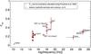 |
Fig. A.1
Measured fractional variability Fvar (black) compared with a delete-d jackknife estimate (red) with |
| Open with DEXTER | |
Almost all light curves of the campaign are unevenly sampled. The sampling is different for each instrument depending on observation schedule, weather and technical issues. There are often gaps of different lengths in the light curves and each light curve has a different number of data points ranging from a few up to a few hundred. In addition, some light curves are binned into bins of several days because of the limited sensitivity of the corresponding instruments. Therefore we have to assess whether there is an error introduced to Fvar by the uneven sampling and the binning and how the Fvar values can be compared. In addition we need to know the minimum number of flux measurements per light curve which are needed to obtain a reliable, unbiased Fvar value.
To address these questions, we first made a delete-d jackknife analysis, i.e., from each light curve containing N data points, we randomly removed d data points (1 ≤ d ≤ N − 2) and calculated Fvar for this reduced sample of N − d data points. Applying a delete-d jackknife analysis on a time series is formally not correct, as the data are correlated in time (blazar light curves usually show a red-noise behavior). However, our purpose is to create datasets that have statistical properties
identical to the real data to demonstrate the impact of gaps and uneven sampling on Fvar. Figure A.1 shows Fvar for the jackknife datasets with ![]() in comparison with Fvar for the original light curves. The Fvar values do not change significantly. The error bars are larger because of the reduced number of flux values in the jackknife samples. The result does not depend on the particular choice of d, as long as there are sufficient datapoints in the jackknife-samples remaining. Some of the light curves are (almost) regularly sampled, namely Fermi-LAT, RXTE/PCA and RXTE/ASM. These are good examples that demonstrate that irregular sampling does not introduce a bias to the Fvar measurement.
in comparison with Fvar for the original light curves. The Fvar values do not change significantly. The error bars are larger because of the reduced number of flux values in the jackknife samples. The result does not depend on the particular choice of d, as long as there are sufficient datapoints in the jackknife-samples remaining. Some of the light curves are (almost) regularly sampled, namely Fermi-LAT, RXTE/PCA and RXTE/ASM. These are good examples that demonstrate that irregular sampling does not introduce a bias to the Fvar measurement.
We also varied d between 1 and N − 2. Figure A.2 shows Fvar vs. (N − d) /N for selected light curves. As long as N − d is larger than ~5, the measured Fvar is approximately constant with varying d and in agreement with Fvar of the original light curve. Likewise, the error bars do not change significantly. Strong deviations from Fvar of the original light curve occur only, if at all, when N − d< 10. No significant deviations are observed at N − d ≥ 20 for any of the light curves. Thus we conclude that our Fvar measurement is robust for all light curves with 20 or more flux data points. In our multi-wavelength sample most light curves in the optical, UV, X-rays, HE γ rays and VHE have more than 20 flux data points. In the radio and near-infrared, most light curves do not.
Fvar is reliable for all but the smallest samples. If after removal of d data points the remaining sample is smaller than about 10, then Fvar might be over- or underestimated.
We also made a moving-block jackknife test, i.e., we removed blocks of m consecutive measurements. This test is still formally correct when the data are slightly correlated in time, but the drawback is that the number of jackknife samples is much smaller than in case of the delete-d jackknife test. Likewise, it only shows the influence of gaps, not the influence of a random sampling. Figure A.3 shows the test for ![]() . As in the case of the delete-d jackknife test, the Fvar values do not change significantly and the uncertainties are larger.
. As in the case of the delete-d jackknife test, the Fvar values do not change significantly and the uncertainties are larger.
These conclusions, however, are only valid because the dataset does not have any strong flare and hence it is unaffected by removing points or blocks randomly. Occasional strong flares therefore should be removed before doing an Fvar analysis of light curves that are otherwise in a typical or low state.
|
Fig. A.2
Fractional variability Fvar (red) as a function of (N − d) /N for the jackknife-d samples of selected representative light curves. The measured Fvar of the original light curve and its error are shown as red horizontal lines. The Fvar of the jackknife-samples is constant and agrees with the original Fvar within its errors for all but the largest d (i.e., the smallest jackknife-samples). |
|
| Open with DEXTER | |
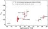 |
Fig. A.3
Measured fractional variability Fvar (black) compared with a moving-block jackknife estimate (red), using a blocksize of |
| Open with DEXTER | |
© ESO, 2015
Current usage metrics show cumulative count of Article Views (full-text article views including HTML views, PDF and ePub downloads, according to the available data) and Abstracts Views on Vision4Press platform.
Data correspond to usage on the plateform after 2015. The current usage metrics is available 48-96 hours after online publication and is updated daily on week days.
Initial download of the metrics may take a while.